The Spectra of IceCube Neutrino (SIN) candidate sources - II. Source Characterisation

Abstract

Eight years after the first detection of high-energy astrophysical neutrinos by IceCube we are still almost clueless as regards to their origin, although the case for blazars being neutrino sources is getting stronger. After the first significant association at the $3-3.5\,\sigma$ level in time and space with IceCube neutrinos, i.e. the blazar TXS 0506+056 at $z=0.3365$, some of us have in fact selected a unique sample of 47 blazars, out of which $\sim 16$ could be associated with individual neutrino track events detected by IceCube. Building upon our recent spectroscopy work on these objects, here we characterise them to determine their real nature and check if they are different from the rest of the blazar population. For the first time we also present a systematic study of the frequency of masquerading BL Lacs, i.e. flat-spectrum radio quasars with their broad lines swamped by non-thermal jet emission, in a $\gamma$-ray- and IceCube-selected sample, finding a fraction $>$ 24 per cent and possibly as high as 80 per cent. In terms of their broad-band properties, our sources appear to be indistinguishable from the rest of the blazar population. We also discuss two theoretical scenarios for neutrino emission, one in which neutrinos are produced in interactions of protons with jet photons and one in which the target photons are from the broad line region. Both scenarios can equally account for the neutrino-blazar correlation observed by some of us. Future observations with neutrino telescopes and X-ray satellites will test them out.

1 Introduction

The observation of ultra-high energy cosmic rays (CRs) by the Pierre Auger Observatory (PAO) and Telescope Array (TA) has revealed the existence of extreme cosmic accelerators but not yet their nature and location in the Universe (see, e.g. Anchordoqui, 2019, and references therein). Complementary to the PAO and TA observations the IceCube Neutrino Observatory at the South Pole has detected tens of neutrinos of likely astrophysical and extragalactic origin with energies extending beyond 1 PeV ($10^{15}$ eV) (e.g. Schneider, 2019; Stettner, 2019; Aartsen et al., 2020a, and references therein). Neutrinos of such high energies are most likely generated by the interaction of very high-energy (VHE) CRs with matter or radiation, which leads to the production of charged and neutral mesons, which then decay into neutrinos, $\gamma$-rays, and other particles. This has at least two important astronomical implications: (1) at variance with CRs, which, being charged, get deflected, and $\gamma$-rays, which are absorbed by pair-production interactions with the extragalactic background light (EBL) at $E\gtrsim 100$ GeV (Gould & Schréder 1967; see also, e.g. Biteau et al. 2020 and references therein), neutrinos can travel cosmological distances basically unaffected by matter and magnetic fields and are the only “messengers”, which can provide information on the VHE physical processes that generated them. Said differently, the extragalactic photon sky is almost completely dark at the energies sampled by IceCube ($\gtrsim 60$ TeV); (2) the presence of PeV neutrinos implies the existence of protons up to energies $\gtrsim 10^{17}$ eV. This has huge implications for the study of high-energy emission processes in astronomical sources.

Various astrophysical classes have been suggested to be responsible for the observed IceCube signal (e.g. Ahlers & Halzen, 2015, and references therein). The absence of a significant anisotropy is consistent with the majority ($\gtrsim 85$ per cent) of the neutrino flux being due to extragalactic population(s) (e.g. Aartsen et al., 2017c, 2019). So far, however, only one astronomical source has been significantly associated (at the $3-3.5\,\sigma$ level) in time and space with IceCube neutrinos, i.e. the blazar TXS 0506+056 at $z=0.3365$ (IceCube Collaboration et al., 2018a; IceCube Collaboration, 2018b; Padovani et al., 2018; Paiano et al., 2018). Aartsen et al. (2020a) have also reported an excess of neutrinos at the $2.9\,\sigma$ level from the direction of the local ($z=0.004$) Seyfert 2 galaxy NGC 1068 and a $3.3\,\sigma$ excess in the northern sky due to significant p-values in the directions of NGC 1068 and three blazars: TXS 0506+056, PKS 1424+240, and GB6 J1542+6129. Moreover, Stein et al. (2021) have presented the association of a radio-emitting tidal disruption event (AT2019dsg) with a high-energy neutrino, giving a probability of finding such an event by chance $\sim 0.5$ per cent, which decreases to $\sim 0.2$ per cent ($\sim 2.9\,\sigma$) if one takes into account its bolometric flux. Very recently, IceCube collaboration et al. (2021) have performed a search for flare neutrino emission in the 10 years of IceCube data and reported a cumulative time-dependent neutrino excess in the northern hemisphere at the level of 3 $\sigma$ associated with four sources: a radio galaxy, M87, two blazars (TXS 0506+056 and GB6 J1542+6129) and the Seyfert 2 galaxy (NGC 1068), these last three sources also being associated with neutrinos by Aartsen et al. (2020a). Blazars are a rare class of Active Galactic Nuclei (AGN; see Falomo, Pian, & Treves, 2014; Padovani et al., 2017, for reviews) having a relativistic jet that is pointing very closely to our line of sight (e.g. Urry & Padovani, 1995; Padovani et al., 2017). The case for a sub-class of blazars being neutrino sources, however, is mounting (see also Righi, Tavecchio, & Inoue, 2019). Giommi et al. (2020a) (hereafter G20), have carried out a detailed dissection of all the public IceCube high-energy neutrinos that are well reconstructed (so-called tracks) and off the Galactic plane, which provided a $3.2\,\sigma$ (post-trial) correlation excess with $\gamma$-ray detected IBLs and HBLs. No excess was found for LBLs. Given that TXS 0506+056 is also a blazar of the IBL/HBL type (Padovani et al., 2019) this result, together with previous findings, consistently points to growing evidence for a connection between some IceCube neutrinos and IBL and HBL blazars. We note that some papers have also found correlations with LBLs rather than IBLs/HBLs both through statistical tests and studies of individual sources (e.g. Kadler et al., 2016; Hovatta et al., 2021; Plavin et al., 2020, 2021, we discuss these and other papers in Section 7.4).

Based on the results of G20, out of the 47 IBLs and HBLs in their Table 5, $16\pm 4$ could be new neutrino sources waiting to be identified. Further progress requires optical spectra, which are needed to measure the redshift, and hence the luminosity of the source, determine the properties of the spectral lines, and possibly estimate the mass of the central black hole, $M_{\rm BH}$.

Paiano et al. (2021) (hereafter Paper I) presented the spectroscopy of a large fraction of the objects selected by G20, which, together with results taken from the literature, covered $\sim 80$ per cent of that sample. Paper I is the first publication of the project entitled “The spectra of IceCube Neutrino (SIN) candidate sources” whose aim is threefold: (1) determine the nature of the sources; (2) model their SEDs using all available multi-wavelength data and subsequently the expected neutrino emission from each blazar; (3) determine the likelihood of a connection between the neutrino and the blazar using a physical model for the blazar multi-messenger emissions, as done, for example, by some of us in Petropoulou et al. (2015, 2020).

The purpose of this paper is to characterise the sources studied in Paper I, to determine their real nature, extending the work done by Padovani et al. (2019) for TXS 0506+056 to a much larger sample of possible neutrino sources, and also see if these sources are any different from the rest of the blazar population. Given that only less than half of our sample is expected to be associated with IceCube tracks, this last point might not be very straightforward. Although the paper is data-driven, we nevertheless perform also a preliminary theoretical analysis of our sample.

The paper is structured as follows: Section 2 describes the sample we used, while Section 3 deals with ancillary data. In Section 4 we present our main results on the source characterisation, Section 5 deals with some additional sources, while Section 6 gives a theoretical interpretation of our results in the context of high-energy neutrino emission. Finally, Section 7 discusses our results and Section 8 summarises our conclusions. In Appendix A we describe how we estimate $M_{\rm BH}$. We use a $\Lambda$CDM cosmology with Hubble constant $H_{0}=70$ km s^-1 Mpc^-1, matter density $\Omega_{\rm m,0}=0.3$, and dark energy density $\Omega_{\Lambda,0}=0.7$. Spectral indices are defined by $S_{\nu}\propto\nu^{-\alpha}$ where $S_{\nu}$ is the flux at frequency $\nu$.

2 The sample

Paper I combined a literature search with newly obtained spectra and presented redshifts for 36 IBLs and HBLs on the G20’s list (see Tables 1 and 3 therein). These form the basis of our sample, which also includes two sources, 5BZB J1322+3216 and 3HSP J152835.7+20042, for which we derived an estimate of the redshift as discussed in Appendix A and from the host galaxy contribution to the SED (see, e.g. Chang et al., 2019), respectively. In the following, we refer to these two redshift estimates as “photometric” for brevity. To these, we further add M87 and 3HSP J095507.9+35510 (Giommi et al., 2020b), an extreme blazar associated with an IceCube track, which was announced after the G20 paper was completed but which still fulfils all the criteria for the sample construction of that paper. These 40 objects are all $\gamma$-ray detected and have been chosen by selection to have $|b_{\rm II}|>10^{\circ}$ and (M87 excluded) $\nu_{\rm peak}^{S}$ $>10^{14}$ Hz. The G20’s sources are matched to 30 neutrino events out of 70 having an area of the error ellipse smaller than that of a circle with radius r $=3^{\circ}$. More than one blazar is within the IceCube error ellipse in most cases. Finally, Paper I presented also the spectra of some additional targets included in a preliminary version of the G20’s list. These were still $\gamma$-ray emitting blazars without a redshift determination, which turned out not to fulfil all the final criteria adopted by those authors. In the following we refer to these sources as the “extra” sources and discuss those with $\nu_{\rm peak}^{S}$ $>10^{14}$ Hz in Section 5. Given their “additional” nature these sources are not included in the statistical analysis of Section 4.

3 Ancillary data

3.1 Radio data and $\nu_{\rm peak}^{S}$

Radio flux densities at 1.4 GHz are given in Table 5 of G20 and span the range $0.003-1$ Jy. These come from radio catalogues and therefore represent typical values. $\nu_{\rm peak}^{S}$ values have been estimated on the basis of the multifrequency data from the catalogues and spectral databases called by the VOU_Blazars tool V1.92 (Chang, Brandt, & Giommi, 2020), time averaged when multiple observations at the same frequency were present (see also Section 3.2 of G20). Since IBLs and HBLs are known to be highly variable both in flux and $\nu_{\rm peak}^{S}$, the estimation of the latter parameter, especially for those objects for which only sparse data are available, may change, even significantly, when additional data become available. Radio powers at 1.4 GHz, assuming a flat radio spectrum ($\alpha_{\rm r}=0$), and $\nu_{\rm peak}^{S}$ values (rest-frame, i.e. multiplied by $(1+z)$) are given in Table 1.

3.2 Optical data

Paper I has presented optical spectroscopy secured at the Gran Telescopio Canarias and at the ESO Very Large Telescope for 17 sources in the G20’s sample with unknown redshift. The latter was determined for nine objects, spanning the $0.09-1.6$ range, while for the others lower limits were derived based either on the absence of spectral signatures of the host galaxy or intervening absorption systems. Forbidden and semi-forbidden emission lines with powers in the range $\sim 10^{40}-4\times 10^{41}$ erg s^-1 were also detected.

3.2.1 Additional optical data

Spectra for twelve additional sources were retrieved from the Sloan Digital Sky Survey (SDSS: Ahumada et al., 2020) and ZBLLAC database and were used to measure the line luminosity of, or an upper limit to, [O iii] 5007 Å and [O ii] 3727 Å. The latter was derived by simulating the emission features at the expected line position for a range of equivalent widths, setting the upper limit based on the signal to noise of the spectrum at the relevant wavelength. [O iii] and [O ii] lines were detected in three and two objects respectively. All [O iii] and [O ii] line powers are given in Table 1.

3.2.2 Disc luminosities for additional sources

For five sources for which we had no line information we got an upper limit on $L_{\rm disc}$ from Paliya et al. (2021). This was used to derive an upper limit on the accretion-related bolometric luminosity (Section 4). These sources have no $L_{\rm[\text{O\,{ii}}]}$ and $L_{\rm[\text{O\,{iii}}]}$ entries and an upper limit in Table 1 on the Eddington ratio, i.e, the ratio between the (accretion-related) observed luminosity and the Eddington luminosity, $L_{\rm Edd}=1.26\times 10^{46}~{}(M/10^{8}\rm M_{\odot})$ erg s^-1, where $\rm M_{\odot}$ is one solar mass.

3.2.3 Black hole masses

The optical spectrum of our sources is typically made up of a non-thermal component superposed on the host galaxy spectrum (see, e.g. Falomo, Pian, & Treves, 2014). When possible, we have therefore decomposed the observed optical spectra into a power-law plus a template spectrum for the host galaxy following Mannucci et al. (2001). The decomposition was obtained from a best fit assuming two free parameters: the nucleus-to-host ratio and the spectral slope of the non-thermal component. This decomposition yields a good representation of the observed spectra, with a ratio of the two components, evaluated at 6500 Å, ranging from 0.3 to 5 (with a median value of 2.5). From the observed magnitude of the host galaxy in the R band we then computed the absolute magnitude $M(R)$ including the k-correction and a correction for passive (i.e. with the bulk of the stars formed at high redshift) evolution (Bressan, Granato, & Silva, 1998) in order to properly match the observations with local Universe data. Finally, we estimated $M_{\rm BH}$ for these sources using the $M_{\rm BH}-M(R)$ relationship of Labita et al. (2007) (consistent with the one by McLure & Dunlop (2002) for the same cosmological parameters), which gives a typical uncertainty $\approx 0.45$ dex (we refer the reader to Appendix A for more details). The mass for M87 is from Event Horizon Telescope Collaboration et al. (2019), the upper limit on the mass of TXS 0506+065 assumes the host galaxy to be a typical giant elliptical with $M(R)\sim-22.9$, or fainter (see discussion in Padovani et al., 2019), while for CRATES J232625+011147 we use the mass obtained by Paliya et al. (2021) by applying the virial technique to the Mg ii line. For the 35 per cent of the sources for which we could not estimate $M_{\rm BH}$ we adopt $M_{\rm BH}=6.3\times 10^{8}M_{\odot}$, which assumes the host galaxy to be a typical giant elliptical (Labita et al., 2007), a value which is very close to the median of our masses ($M\sim 4\times 10^{8}M_{\odot}$). $M_{\rm BH}$ values are reported in Table 1 and detailed in Table LABEL:tab:apdx.

3.3 $\gamma$-ray data

The analysis of the sources’ $\gamma$-ray emission is based on Fermipy (Wood et al., 2017) and uses publicly available Fermi-LAT Pass 8 data (with the P8R3_SOURCE_V3 instrument response function) acquired in the period August 4, 2008 to mid 2020 and follows the standard procedures suggested by the Fermi-LAT team. Namely, we select only events with a high probability of being photons (evclass = 128, evtype = 3 [FRONT+BACK]) in the energy range between 100 MeV and 300 GeV from a region of interest (ROI) of 20^∘ around the source’s position. Possible contamination from the Earth limb is removed by cutting out events with zenith angle $>90^{\circ}$ and only considering time intervals in which the data acquisition of the spacecraft was stable (DATA_QUAL>0 && LAT_CONFIG==1).

Each fit is based on an emission model that, besides the target source at its multi-frequency position, incorporates the isotropic (gll_iem_v07) and Galactic (iso_P8R3_SOURCE_V3_v1) diffuse component, as well as all the known $\gamma$-ray point sources in the region. In addition to the spectral parameters of the target source the flux normalisation of the diffuse component and the spectral parameters of all point and extended sources within $\sim$ 13^∘ (95 per cent point spread function at 100 MeV) are treated as free parameters. This procedure thereby efficiently reduces the risk of source confusion. Finally, the best-fit flux of the target source is determined by maximising the signal likelihood $\mathcal{L}(\textrm{full\,model | data})$. For the significance we further maximise the background likelihood $\mathcal{L}(\textrm{bkg\,model | data})$, i.e. the model without the target source. The test-statistic is then defined as

$$TS=2\times\left[\log\mathcal{L}(\textrm{full\,model | data})-\log\mathcal{L}(\textrm{bkg\,model | data})\right].$$ (1)

The TS value can be converted to a significance using the $\chi^{2}$ distribution with two-degrees of freedom. We can then confirm the significant detection (well $>3\,\sigma$) of all but two sources in our sample independently of the Fermi-LAT Fourth Source Catalog (4FGL: Abdollahi et al. 2020). The remaining two objects, i.e. 3HSP J062753.3$-$15195 (3FGL J0627.9$-$1517) and 3HSP J125821.5+21235 (3FGL J1258.4+2123), have dropped to 2.1 and 2.5$\,\sigma$ for the time-integrated emission (down from $\sim 4.5$ and 5.0$\,\sigma$, respectively) and are not included in the Fermi-4FGL-DR2 catalogue (Ballet et al., 2020). This drop in significance is characteristic for strongly time-variable objects and therefore not unexpected. Furthermore, visual inspection shows that the multi-wavelength SEDs are fully-consistent with the derived $\gamma$-ray spectra. Rest-frame, k-corrected, $\gamma$-ray powers between 0.1 and 100 GeV, $L_{\gamma}$, were then derived by integrating the best-fit spectra, together with $1\,\sigma$ statistical uncertainties.

Table 1: Main sample properties.

Name	4FGL name	$z$	$\nu_{\rm peak}^{S}$	$P_{\rm 1.4GHz}$	$L_{\rm[\text{O\,{ii}}]}$	$L_{\rm[\text{O\,{iii}}]}$	$M_{\rm BH}$	$L/L_{\rm Edd}$	$L_{\gamma}/L_{\rm Edd}$
			[Hz]	[W Hz-1]	[erg s-1]	[erg s-1]	[$M_{\odot}$]
3HSP J010326.0+15262	4FGL J0103.5+1526	0.2461	15.1	25.52	<40.8	40.9	8.6	-1.8	-2.1
5BZU J0158+0101	4FGL J0158.8+0101	0.4537	14.3	25.63	<41.0	40.7	7.4	-0.8	-0.1
VOU J022411+161500	4FGL J0224.2+1616	>0.5	14.7	>24.93	…	…	…	…	>-1.5
3HSP J023248.5+20171	4FGL J0232.8+2018	0.139	18.6	24.58	…	…	8.8	<-3.4	-2.7
3HSP J023927.2+13273	4FGL J0239.5+1326	>0.7	15.2	>25.41	…	…	…	…	>-1.4
CRATES J024445+132002	4FGL J0244.7+1316	0.9846	14.8	26.55	41.6	…	…	-1.3	-0.6
3HSP J033913.7$-$17360	4FGL J0339.2$-$1736	0.066	15.6	24.23	…	…	8.6	<-3.0	-2.8
3HSP J034424.9+34301	4FGL J0344.4+3432	>0.25	15.8	>24.29	…	…	…	…	>-2.4
TXS 0506+056	4FGL J0509.4+0542	0.3365	14.6	26.18	41.3	41.3	<8.8	>-1.7	>-0.4
CRATES J052526$-$201054	4FGL J0525.6$-$2008	0.0913	14.5	24.64	…	40.3	8.1	-1.7	-2.7
3HSP J062753.3$-$15195	3FGL J0627.9$-$1517	0.3102	17.4	25.01	<41.1	<40.8	9.0	<-2.0	-2.6
3HSP J064933.6$-$31392	4FGL J0649.5$-$3139	>0.7	17.2	>24.98	…	…	0.0	…	>-1.0
3HSP J085410.1+27542	4FGL J0854.0+2753	0.493	16.3	24.96	…	…	9.0	<-2.5	-2.5
3HSP J094620.2+01045	4FGL J0946.2+0104	0.576	>18.2	25.11	<41.7	<40.5	8.6	<-1.6	-1.0
3HSP J095507.9+35510	4FGL J0955.1+3551	0.557	17.9	24.81	<40.3	<40.3	8.8	<-2.0	-1.7
GB6 J1040+0617	4FGL J1040.5+0617	0.74	14.7	25.70	41.0	…	…	-1.5	-0.2
5BZB J1043+0653	4FGL J1043.6+0654	>0.7	14.7	>25.00	…	…	…	…	>-1.3
3HSP J111706.2+20140	4FGL J1117.0+2013	0.138	16.6	24.66	40.7	<40.4	8.1	-0.9	-1.3
M87	4FGL J1230.8+1223	0.0043	…	a22.60	…	…	b9.8	<-6.2	-6.1
3HSP J123123.1+14212	4FGL J1231.5+1421	0.2558	16.1	24.95	<41.2	<40.9	8.4	<-1.4	-1.7
3HSP J125821.5+21235	3FGL J1258.4+2123	0.6265	16.9	25.43	<41.1	…	8.0	<-0.7	-1.2
3HSP J125848.0$-$04474	4FGL J1258.7$-$0452	0.4179	17.2	24.28	<40.5	<40.3	8.4	<-1.6	-1.3
3HSP J130008.5+17553	4FGL J1300.0+1753	>0.6	14.7	>25.18	…	…	…	…	>-1.6
5BZB J1314+2348	4FGL J1314.7+2348	0.15c	>14.1	24.99	…	…	…	…	-2.1
5BZB J1322+3216	4FGL J1321.9+3219	0.4d	14.6	26.56	…	…	8.2	<-2.1	-1.4
VOU J135921$-$115043	4FGL J1359.1$-$1152	0.242	14.1	24.83	…	<40.3	8.6	<-2.1	-2.7
3HSP J140449.6+65543	4FGL J1404.8+6554	0.3627	16.1	24.71	<41.0	<40.8	8.3	<-1.3	-1.1
VOU J143934$-$252458	4FGL J1439.5$-$2525	0.16	14.1	24.32	…	…	8.6	<-3.1	-2.6
3HSP J143959.4$-$23414	4FGL J1440.0$-$2343	0.309	16.3	25.38	40.9	40.5	8.6	-1.7	-1.6
3HSP J144656.8$-$26565	4FGL J1447.0$-$2657	0.3315	17.7	25.05	<40.5	<40.4	8.6	<-1.8	-2.0
3HSP J152835.7+20042	4FGL J1528.4+2004	0.52d	16.4	24.39	…	…	…	…	-1.8
3HSP J153311.2+18542	4FGL J1533.2+1855	0.307	17.1	24.73	<41.3	<40.9	8.4	<-1.4	-1.6
3HSP J155424.1+20112	4FGL J1554.2+2008	0.2223	17.4	24.98	<40.9	<40.5	8.6	<-1.8	-2.2
3HSP J180849.7+35204	4FGL J1808.8+3522	0.141	15.1	24.15	<40.5	<40.3	8.0	<-1.2	-2.3
3HSP J213314.3+25285	4FGL J2133.1+2529	0.294	15.3	24.93	…	…	8.8	…	-2.0
3HSP J222329.5+01022	4FGL J2223.3+0102	>0.7	15.7	>24.94	…	…	…	…	>-1.4
5BZB J2227+0037	4FGL J2227.9+0036	>1.0935	14.8	>26.50	…	…	…	…	>-0.2
CRATES J232625+011147	4FGL J2326.2+0113	1.595	14.4	27.12	…	…	9.3	-2.7	-0.7
3HSP J235034.3$-$30060	4FGL J2350.6$-$3005	0.2328	15.8	24.70	…	…	…	…	-2.1
IC 5362	4FGL J2351.4$-$2818	0.0276	14.5	23.19	…	…	…	…	-4.6

Notes. All values, apart from redshift, are in logarithmic scale; ^atime-averaged VLBA core power at 15 GHz (Kim et al., 2018);
^bEvent Horizon Telescope Collaboration et al. (2019); ^cuncertain redshift; ^dphotometric redshift. Masquerading BL Lacs are indicated in bold face, while non-masquerading ones in italics.

4 Source characterisation

We now characterise our sources using the data discussed above. The main issue we want to address is that of the so-called “masquerading” BL Lacs. Padovani et al. (2019) showed that TXS 0506+056, the first plausible non-stellar neutrino source is, despite appearances, not a blazar of the BL Lac type but instead a masquerading BL Lac. This class was introduced by Giommi et al. (2012a); Giommi, Padovani, & Polenta (2013) (see also Ghisellini et al. 2011) and includes sources which are in reality FSRQs whose emission lines are washed out by a very bright, Doppler-boosted jet continuum, unlike “real” BL Lacs, which are intrinsically weak-lined objects. This is relevant because “real” BL Lacs and FSRQs belong to different physical classes, i.e. objects without and with high-excitation emission lines in their optical spectra, referred to as low-excitation (LEGs) and high-excitation galaxies (HEGs), respectively. TXS 0506+056, being a HEG, therefore benefits from several radiation fields external to the jet (i.e. the accretion disc, photons reprocessed in the broad-line region or from the dusty torus), which, by providing more targets for the protons might enhance neutrino production as compared to LEGs. This makes masquerading BL Lacs (and, at first glance, FSRQs: see Section 7.4) particularly attractive from the point of view of high-energy neutrinos.

As per Padovani et al. (2019), to which we refer the reader for more details, we use the following parameters to look for masquerading BL Lacs, i.e. BL Lacs with HEG-like (i.e. quasar-like) properties, in our sample, in decreasing order of relevance:

1. the location on the radio power – emission line power, $P_{\rm 1.4GHz}$ – $L_{\rm[\text{O\,{ii}}]}$, diagram (Fig. 4 of Kalfountzou et al., 2012), which defines the locus of jetted (radio-loud) quasars. Any BL Lac falling on this locus has to be a masquerading one, while real BL Lacs will occupy the lower-left part of the plot. This is quite straightforward but requires the detection (or an upper limit on the flux) of the [O ii] 3727 Å line;

2. a radio power $P_{\rm 1.4GHz}>10^{26}$ W Hz^-1, since HEGs become the dominant population in the radio sky above this value (Heckman & Best, 2014). Although this is strictly valid for the local Universe, it can be applied to higher redshifts as well because LEGs do not evolve much in luminosity, unlike HEGs (e.g. Padovani et al., 2015a). Note that there are many HEGs below this limit so the fact that a source does not satisfy this condition does not rule out a masquerading BL Lac classification;

3. an Eddington ratio $L/L_{\rm Edd}\gtrsim 0.01$, which is typical of HEGs. The derivation of the thermal, accretion-related bolometric luminosity is not that easy for BL Lacs and it involves measuring $L_{\rm[\text{O\,{ii}}]}$ and $L_{\rm[\text{O\,{iii}}]}$ (e.g. Punsly & Zhang, 2011). In the case of CRATES J232625+011147, at $z=1.595$, we used its Mg ii and C iii] luminosities to estimate the broad-line region (BLR) luminosity, $L_{\rm BLR}$, from the composite spectrum of Vanden Berk et al. (2001) (we then derived $L_{\rm disc}\sim 10\times L_{\rm BLR}$ assuming a standard covering factor of $\sim 10$ per cent and $L\sim 20\times L_{\rm BLR}$: see Padovani et al. 2019). The upper limit for M87 has been derived from its limit on $L_{\rm BLR}$ (Sbarrato, Padovani, & Ghisellini, 2014), while the upper limits on $L_{\rm disc}$ from Paliya et al. (2021) (Section 3.2.2) turned into upper limits on $L<2\times L_{\rm disc}$ (Padovani et al., 2019). $L_{\rm Edd}$ requires an estimate of the black hole mass, which is not straightforward to get (Section 3.2.3);

4. a $\gamma$-ray Eddington ratio $L_{\gamma}/L_{\rm Edd}\gtrsim 0.1$, following Sbarrato et al. (2012) who have proposed a division between “real” BL Lacs and FSRQs at this value. As is the case for $L/L_{\rm Edd}$ this also requires an estimate of the black hole mass.

   Padovani et al. (2019) derived also $L_{\rm BLR}/L_{\rm Edd}$, which was needed to estimate the $\gamma$-ray attenuation due to the BLR photon field. However, for BL Lacs the estimation of $L_{\rm BLR}$ depends on $L_{\rm[\text{O\,{ii}}]}$ and $L_{\rm[\text{O\,{iii}}]}$, as is the case for the accretion-related bolometric luminosity, and therefore this is not an independent parameter to characterise a source. Nonetheless, we do use $L_{\rm BLR}$ in one of our theoretical scenarios in Section 6.2.

We apply these four criteria in descending order of importance. We anticipate that no object is classified as masquerading based only on $L/L_{\rm Edd}$ and/or $L_{\gamma}/L_{\rm Edd}$, which are the least certain parameters given their $L$ and $M_{\rm BH}$ dependence. In practice, then, the Eddington ratios are used only as a consistency check.

Table 2: Masquerading BL Lac properties: main sample.

Name	IceCube Name	$z$	$P_{\rm 1.4GHz}-L_{\rm\text{O\,{ii}}}$	$P_{\rm 1.4GHz}$	$L/L_{\rm Edd}$	$L_{\gamma}/L_{\rm Edd}$
3HSP J010326.0+15262	IC160331A	0.2461	✓	I	✓	✗
5BZU J0158+0101	IC090813A	0.4537	✓	I	✓	✓
TXS 0506+056	IC170922A	0.3365	✓	✓	✓	✓
CRATES J052526$-$201054	IC150428A	0.0913	✓	I	✓	✗
GB6 J1040+0617	IC141209A	0.74	✓	I	✓	✓
3HSP J111706.2+20140	IC130408A	0.1380	✓	I	✓	✗
3HSP J143959.4$-$23414	IC170506A	0.309	✓	I	✓	✗
5BZB J2227+0037	IC140114A	>1.0935	–	✓	–	✓
CRATES J232625+011147	IC160510A	1.595	–	✓	✗	✓

Notes. “I” implies that the condition is not met but this does not mean this is not a masquerading BL Lac, –” that no information is available.

Table 1 gives the main properties of the sample, namely name (column 1), Fermi-4FGL name (column 2), redshift (column 3), rest-frame $\nu_{\rm peak}^{S}$ (column 4), $P_{\rm 1.4GHz}$ (column 5), $L_{\rm[\text{O\,{ii}}]}$ and $L_{\rm[\text{O\,{iii}}]}$ (columns 6 and 7), $M_{\rm BH}$ (column 8), $L/L_{\rm Edd}$ and $L_{\gamma}/L_{\rm Edd}$ (columns 9 and 10). When $M_{\rm BH}$ is missing we assumed a value of $6.3\times 10^{8}M_{\odot}$, as discussed above. Masquerading BL Lacs are indicated in bold face, non-masquerading ones in italics, while sources for which we do not have the relevant information to make a decision are in roman (Section 7.2). More details on masquerading BL Lacs are given in Table 2. We refer the reader to Tables 1 and 3 of Paper I for redshift references and details on the spectra. Note that all but one redshift lower limits have been derived from the lack of detection of host galaxy absorption lines assuming a standard elliptical host galaxy with $M(R)=-22.9$, the remaining limit (for 5BZB J2227+0037) being instead based on the detection of intervening absorption systems attributed to Mg II and Fe II.

4.1 The radio power – emission line diagram ($P_{\rm 1.4GHz}$ – $L_{\rm[\text{O\,{ii}}]}$)

Fig. 1 shows the location of the sources with [O ii] information on the $P_{\rm 1.4GHz}$ – $L_{\rm[\text{O\,{ii}}]}$ diagram. To increase our statistics we have also added two objects for which only the [O iii] flux was available, converting $L_{\rm[\text{O\,{iii}}]}$ to $L_{\rm[\text{O\,{ii}}]}$ using the scaling relation $L_{\rm[\text{O\,{ii}}]}\propto L_{\rm[\text{O\,{iii}}]}^{0.04}$, as implied by Fig. 7 of Kalfountzou et al. (2012) (see the red line therein; these sources are marked differently in the figure). Seven objects are close to the locus of jetted AGN and are therefore “bona fide” masquerading BL Lacs. These include, apart from TXS 0506+056, 3HSP J010326.0+15262, 5BZU J0158+0101, CRATES J052526$-$201054, GB6 J1040+0617, 3HSP J111706.2+20140, and 3HSP J143959.4$-$23414. All have also $L/L_{\rm Edd}\geq 0.01$. Two of these objects (3HSP J010326.0+15262 and 5BZU J0158+0101) have upper limits on their $L_{\rm[\text{O\,{ii}}]}$, although quite close to the locus, but we still classify them as masquerading because they have an [O iii] detection and $L/L_{\rm Edd}\sim 0.014$ and $\sim 0.17$, with the latter source having also $L_{\gamma}/L_{\rm Edd}\sim 0.8$. CRATES J024445+132002, the only FSRQ in our sample, is also (by definition) very close to the locus. Four more sources have quite stringent $L_{\rm[\text{O\,{ii}}]}$ upper limits, while eight more have an upper limit not too far from (or to the right of) the locus. However, given that these latter sources have no other HEG-like property and no [O iii] detection, and that we want to keep the selection conservative, we are not including them with the masquerading sources.

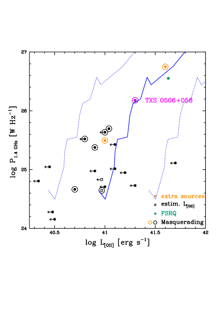
Figure 1: $P_{\rm 1.4GHz}$ vs. $L_{\rm[\text{O\,{ii}}]}$ for our sample (black filled circles), with masquerading sources highlighted (larger empty circles). Sources for which $L_{\rm[\text{O\,{ii}}]}$ has been estimated from $L_{\rm[\text{O\,{iii}}]}$ are denoted by black empty squares. The green filled circle indicates the single FSRQ in our sample, while orange points are the extra sources. TXS 0506+056, which also belongs to our sample, is indicated by a magenta circle. The solid blue line is the locus of jetted (radio-loud) quasars, with the two dotted lines indicating a spread of 0.5 dex, which includes most of the points in Fig. 4 of Kalfountzou et al. (2012) (converted from radio powers in W Hz^-1 sr^-1 and line powers in W). Arrows denote upper limits on $L_{\rm[\text{O\,{ii}}]}$.

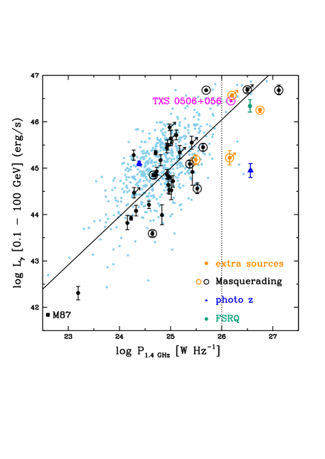
Figure 2: $L_{\gamma}$ vs. $P_{\rm 1.4GHz}$ for our sample (black filled circles), with masquerading sources highlighted (larger empty circles). The green filled circle indicates the single FSRQ, orange points are the extra sources, while the blue triangles denote sources for which we derived an estimate of the redshift from the host galaxy contribution to the SED (see, e.g. Chang et al., 2019). The radio power for M87, which is labelled, is derived from a time-averaged VLBA core flux at 15 GHz (Kim et al., 2018). The average value for TXS 0506+056 (magenta point: Padovani et al. 2019), which also belongs to our sample, is also shown. Error bars denote the uncertainties. The solid line is the linear best fit $L_{\gamma}\propto P_{\rm 1.4GHz}^{1.04}$, while the vertical dotted line marks the $10^{26}$ W Hz^-1 power above which a source is classified as masquerading (see text for details). Arrows denote lower limits on redshift and therefore powers. The small light blue points are the control sample of IBLs and HBLs (see Section 7.1 for details).

4.2 The $\gamma$-ray power – radio power diagram ($L_{\gamma}-P_{\rm 1.4GHz}$)

Fig. 2 shows $L_{\gamma}$ vs. $P_{\rm 1.4GHz}$ for our sources (black circles). We also include the time-averaged very long baseline array (VLBA) core power at 15 GHz for M87 (Kim et al., 2018), which, given its substantially flat radio spectrum between $15-129$ GHz, should be representative of its 1.4 GHz core power as well. Two more sources get classified as masquerading BL Lacs thanks to their $P_{\rm 1.4GHz}>10^{26}$ W Hz^-1, namely 5BZB J2227+0037 and CRATES J232625+011147. Both of them have also $L_{\gamma}/L_{\rm Edd}\gtrsim 0.6$. Note that 5BZB J1322+3216 (a.k.a. 4C+32.43, the rightmost blue triangle) would also have fulfilled (only) the $P_{\rm 1.4GHz}$ criterion but its radio spectrum is very steep ($\alpha_{\rm r}\sim 0.8$ between 130 MHz and 4.8 GHz) and not blazar-like. Its large radio power is therefore due to extended emission and not to the core. This fits with the fact that the host galaxy component is quite visible in its SED and suggests this is a moderately beamed blazar with its non-thermal emission swamped by the galaxy in the radio and near-IR bands (see Giommi et al., 2012a). All other sources have flat radio spectra. Table 2 lists our final list of masquerading BL Lacs with the conditions they fulfil; all sources satisfy at least two criteria.

Fig. 2 shows a very strong linear correlation between the two powers, significant at the $>99.99$ per cent level and with $L_{\gamma}\propto P_{\rm 1.4GHz}^{1.04\pm 0.13}$. (We can exclude that this strong correlation is due to the common redshift dependence of the two powers, as its removal by using a partial correlation analysis (e.g. Padovani, 1992) still gives a 99.8 per cent level significance.) Note that the sample includes also eight sources with lower limits on their redshifts and therefore on their powers. Since the application of survival analysis in this case requires binning, the resulting fit depends on the chosen bin size. We have then tested how this affects our results by increasing artificially the lower limits on the powers by 0.75 dex, which corresponds, for example, to a (large) increase from $z=0.7$ to $z=1.4$. The new best fit is $L_{\gamma}\propto P_{\rm 1.4GHz}^{1.14\pm 0.11}$ with the same significance, fully consistent with our previous results. The issue of how the properties of masquerading sources might differ from those of the other sources is discussed in Section 7.3.

This correlation is not surprising as previous studies have noted the strong $\gamma$-ray – radio correlation for HBLs, stronger than for other blazar sub-classes (e.g. Ackermann et al., 2011a; Lico et al., 2017), and $\sim 62$ per cent of our sources are HBLs. Furthermore, one should expect a correlation between radio and $\gamma$-ray emission in IBLs/HBLs given that their SED is generally consistent with simple one-zone synchrotron self-Compton models with roughly constant ratio between the peak of the Compton and $\nu_{\rm peak}^{S}$ luminosity, the so-called Compton dominance (Abdo et al., 2010; Giommi et al., 2012b). Given that $\nu_{\rm peak}^{S}$ in these sources is located close to the optical band or at higher energies, the ratio between optical and $\gamma$-ray fluxes is close to the Compton dominance, which is similar in most objects. Since the radio to optical spectral slope ($\alpha_{\rm ro}$) in these sources is also known to be approximately constant (Padovani & Giommi, 1995; Abdo et al., 2010) it then follows that the radio and $\gamma$-ray powers are correlated.

4.3 The synchrotron peak – $\gamma$-ray power diagram ($\nu_{\rm peak}^{S}$ – $L_{\gamma}$)

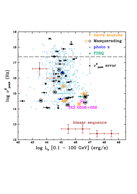
Figure 3: $\nu_{\rm peak}^{S}$ vs. $L_{\gamma}$ for our sample (black filled circles), with masquerading sources highlighted (larger empty circles). The green filled circle indicates the single FSRQ, orange points are the extra sources, while the blue triangles denote sources for which we derived an estimate of the redshift from the host galaxy contribution to the SED (see, e.g. Chang et al., 2019). The average value for TXS 0506+056 (magenta point: Padovani et al. 2019), which also belongs to our sample, and the revised blazar sequence (brown filled squares: Ghisellini et al. 2017) are also shown. Error bars denote the uncertainties (our sources) and the sample dispersion (blazar sequence). The typical $\nu_{\rm peak}^{S}$ uncertainty is also shown (vertical dotted line). Arrows denote lower limits on $\nu_{\rm peak}^{S}$ (vertical) and redshifts (diagonal), which also affect the rest-frame $\nu_{\rm peak}^{S}$ values. Sources above the dashed line are extreme blazars. The small light blue points are the control sample of IBLs and HBLs (see Section 7.1 for details).

Fig. 3 plots the location of our sources (black circles) on the $\nu_{\rm peak}^{S}$ – $L_{\gamma}$ diagram (note that by definition our sample includes only sources with $\nu_{\rm peak}^{S}$ $>10^{14}$ Hz). IBLs cover the $L_{\gamma}\sim 10^{42}-10^{47}$ erg s^-1 range while HBLs occupy the narrower $\sim 10^{44}-10^{46}$ erg s^-1 region all the way up to $\nu_{\rm peak}^{S}$$\sim 3\times 10^{18}$ Hz, although there are also some lower limits on redshift, which means higher $L_{\gamma}$ are very likely. Six sources have $\nu_{\rm peak}^{S}$ $>1$ keV ($2.4\times 10^{17}$ Hz) and are therefore classified as extreme, with one very close at $\nu_{\rm peak}^{S}$ $>1.7\times 10^{17}$ Hz, given its redshift lower limit.

The so-called “blazar sequence” (Fossati et al., 1998; Ghisellini et al., 1998) (see also, e.g. Giommi et al., 2012a, for a detailed discussion and references), posits the existence of a strong anti-correlation between (bolometric) luminosity and $\nu_{\rm peak}^{S}$, related to the apparent lack of FSRQs of the HBL type. Many masquerading BL Lacs fill exactly this void. A number of blazar sequence outliers have also been discovered by different groups (see, e.g. Padovani et al. 2019, for a detailed list and also the very recent paper by Keenan et al. 2021).

Ghisellini et al. (2017) have revisited the original blazar sequence by using the Fermi 3LAC sample (Ackermann et al., 2015), with the result that $\nu_{\rm peak}^{S}$ changes quite abruptly as a function of $L_{\gamma}$, as shown in Fig. 3 (brown filled squares). The same figure (originally shown by Padovani et al. 2019) indicates also the location in its average state (magenta point) of TXS 0506+056, which is an obvious outlier from the sequence. There are three sources quite close to the location of TXS 0506+056, all of them masquerading, plus the FSRQ; two of the extra sources (Section 5), both masquerading, are also in the same region. The issue of how the properties of masquerading sources might differ from those of the other sources is discussed in Section 7.3.

No anti-correlation whatsoever is found between $\nu_{\rm peak}^{S}$ and $L_{\gamma}$, although one could argue that this could be due to the fact that we have a $\nu_{\rm peak}^{S}$ $>10^{14}$ Hz cut. However, while according to the sequence blazars with $L_{\gamma}>10^{45}$ erg s^-1 should typically have $\nu_{\rm peak}^{S}$ $<10^{13}$ Hz, our sources above this power are spread over more than 4 dex in $\nu_{\rm peak}^{S}$ between $10^{14}$ and $\sim 10^{18}$ Hz and occupy a region of parameter space, which is forbidden by the sequence. This happens also at $L_{\gamma}<10^{45}$ erg s^-1, where blazars should typically have $\nu_{\rm peak}^{S}$ $\gtrsim 10^{16}$ Hz while we find a similar spread all the way down to $10^{14}$ Hz, which is the defining limit of our sample.

5 The extra sources

Table 3: Extra sample properties.

Name	4FGL name	$z$	$\nu_{\rm peak}^{S}$	$P_{\rm 1.4GHz}$	$L_{\rm[\text{O\,{ii}}]}$	$L_{\rm[\text{O\,{iii}}]}$	$M_{\rm BH}$	$L/L_{\rm Edd}$	$L_{\gamma}/L_{\rm Edd}$
			[Hz]	[W Hz-1]	[erg s-1]	[erg s-1]	[$M_{\odot}$]
5BZU J1339$-$2401	4FGL J1339.0$-$2400	0.655	14.3	26.75	41.6	41.8	…	-1.5	-0.6
5BZB J1455+0250	4FGL J1455.0+0247	>0.65	14.5	>26.15	…	…	…	…	>-1.7
MG3 J225517+2409	4FGL J2255.1+2411	>0.863	15.0	>26.20	…	…	…	…	>-0.3
NVSS J232538+164641	4FGL J2325.6+1644	0.4817	15.5	25.49	41.0	40.7	…	-1.8	-1.7
Notes. All values, apart from redshift, are in logarithmic scale.

Optical spectra of some targets that were included in a preliminary version of the G20’s list were also presented in Paper I. These are still blazars without a redshift determination, which turned out not to fulfil all the final criteria adopted by the latter authors, especially as regards the size of the IceCube error ellipse and the $\nu_{\rm peak}^{S}$ cut. We discuss here the four sources with $\nu_{\rm peak}^{S}$ $>10^{14}$ Hz with the aim of characterising these sources and looking for other masquerading BL Lacs. These sources are not included in the statistical analysis of Section 4 (but see below for the $L_{\gamma}-P_{\rm 1.4GHz}$ correlation).

Table 4: Masquerading BL Lac properties: extra sample.

Name	IceCube Name	$z$	$P_{\rm 1.4GHz}-L_{\rm\text{O\,{ii}}}$	$P_{\rm 1.4GHz}$	$L/L_{\rm Edd}$	$L_{\gamma}/L_{\rm Edd}$
5BZU J1339$-$2401	IC131202A	0.655	✓	✓	✓	✓
5BZB J1455+0250	IC111201A	>0.65	–	✓	–	–
MG3 J225517+2409	IC100608A	>0.863	–	✓	–	✓
NVSS J232538+164641	IC140522A	0.4817	✓	I	✓	✗

Notes. “I” implies that the condition is not met but this does not mean this is not a masquerading BL Lac, –” that no information is available.

Table 3 gives the main properties of the extra sources, where the columns are the same as in Table 1. Note that the first source is just outside the largest error ellipse considered by G20 (the nominal IceCube major and minor axes scaled by 1.5: Section 7.4), while the other three are associated with events having an area of the error ellipse larger than that of a circle with radius r $=3^{\circ}$. Both sources for which we have $L_{\rm[\text{O\,{ii}}]}$, 5BZU J1339$-$2401 and NVSS J232538+164641, are close to the locus of jetted AGN in Fig. 1 and are therefore “bona fide” masquerading BL Lacs. The former object fulfils all other criteria for such sources, as shown in Table 4, while the latter one has $L/L_{\rm Edd}\sim 0.014$, i.e. it is HEG-like. The other two sources, 5BZB J1455+0250 and MG3 J225517+2409, were classified as masquerading BL Lacs due to their $P_{\rm 1.4GHz}>10^{26}$ W Hz^-1 (Fig. 2), with the second one having also $L_{\gamma}/L_{\rm Edd}>0.5$. In short, all four extra sources are of the masquerading BL Lac type. The extra sources fall on the high $P_{\rm 1.4GHz}$ – high $L_{\gamma}$ side of Fig. 2, as is the case for the other masquerading BL Lacs (see Section 7.3). The best fit including them is still significant at the $>99.99$ per cent level with $L_{\gamma}\propto P_{\rm 1.4GHz}^{0.97\pm 0.12}$, fully consistent with our previous fit ($L_{\gamma}\propto P_{\rm 1.4GHz}^{1.04\pm 0.13}$). As for Fig. 3 the extra sources, again, fall where most masquerading sources are (Section 7.3).

MG3 J225517+2409 has been recently reported as a possible counterpart of five ANTARES track events in the $\sim 3-40$ TeV energy range, on top of being within the (large) error region of the IceCube track IC100608A, with a combined a posteriori ANTARES space-time and IceCube p-value of $2.6\,\sigma$ (Albert et al., 2021). The fact that this source is also a masquerading BL Lac, like TXS 0506+056, is therefore tantalising.

6 Theoretical interpretation

We present here estimates for the expected high-energy neutrino emission from our sample (i.e. 36 IBLs and HBLs with redshift from Paper I, 5BZB J1322+3216 and 3HSP J152835.7+20042, for which we derived a redshift estimate, and 3HSP J095507.9+35510, for a total of 39 sources) within the context of two simplified theoretical scenarios that are summarised below. We also compute the stacked neutrino flux and compare it to the diffuse IceCube neutrino flux.

• Scenario A. High-energy neutrinos are produced by photomeson interactions of relativistic protons with jet synchrotron photons of observed energy $h\nu_{\rm peak}^{S}/(1+z)$ (Mannheim, 1993; Mücke et al., 2003; Petropoulou et al., 2015; Cerruti et al., 2015). The cascade electromagnetic emission, which is induced by photohadronic interactions and photon-photon pair production, has a non-negligible contribution in the Fermi-LAT energy band (see e.g. Figs. 5 and 6 in Petropoulou et al., 2015). This scenario may also apply to masquerading BL Lacs and FSRQs if the neutrino production site lies beyond the BLR (e.g. Gao, Pohl, & Winter, 2017), so that jet radiation provides the main target photon field; for an application to TXS 0506+056 see also Padovani et al. (2019).

• Scenario B. High-energy neutrinos are produced by photomeson interactions of relativistic protons in the jet with the BLR photons of characteristic energy (in the AGN rest frame) $\tilde{\varepsilon}_{\rm BLR}$ (e.g. Atoyan & Dermer, 2001; Murase, Inoue, & Dermer, 2014; Rodrigues et al., 2018). This scenario applies to FSRQs and masquerading BL Lacs, assuming that the neutrino production site lies within the BLR.

6.1 Scenario A

In this scenario photohadronic interactions have an active role in shaping the blazar SED, as detailed in Petropoulou et al. (2015). The low-energy hump of the SED is explained by synchrotron radiation of relativistic electrons in the jet (primary electrons). It is assumed that protons are accelerated to high enough energies (e.g. multi-PeV to EeV energies) as to pion-produce on photons with energy $h\nu_{\rm peak}^{S}/(1+z)$ (in the observer’s frame). The high-energy hump is then explained by a combination of synchrotron-self Compton (SSC) emission from primary electrons and synchrotron emission of electrons and positrons (secondary pairs) produced in photomeson production and photon-photon pair-production processes (henceforth, $p\pi$ component). Since the luminosity of the $p\pi$ cascade component is directly connected to that of high-energy neutrinos, this scenario allows us to associate the observed $\gamma$-ray luminosity with the expected neutrino luminosity of a blazar. Since external radiation fields are not considered in this scenario, the true nature of BL Lac objects in our sample will not be a determining factor in the calculations that follow.

In what follows, we adopt the approach of Padovani et al. (2015b). The bolometric all-flavour neutrino and antineutrino flux of a blazar can be parametrised as

$$F_{\nu+\bar{\nu}}=Y_{\nu\gamma}F_{\gamma},$$ (2)

where $F_{\gamma}=L_{\gamma}/4\pi d_{\rm L}^{2}$ is the $0.1-100$ GeV $\gamma$-ray flux and $d_{\rm L}$ the luminosity distance. We caution the reader that the Fermi/LAT flux alone might not be a good predictor of the expected neutrino numbers, as indicated by recent studies of the neutrino excess from TXS 0506+056 (Reimer, Böttcher, & Buson, 2019; Zhang et al., 2020, and references therein) and pointed out earlier by Krauß et al. (2018). The latter’s conclusion was based on the premise that the integrated neutrino energy flux cannot exceed the integrated electromagnetic energy flux between 0.1 keV and 1 TeV. Given the scatter between Fermi/LAT and 0.1 keV – 1 TeV fluxes (see their Fig. 4), differences of about one order of magnitude in predicted neutrino numbers are possible between models that rely on the broadband or the Fermi/LAT flux as proxies for the neutrino flux. More complex scenarios are certainly also viable, such as the production of TeV - PeV neutrinos in coincidence with X-ray flares powered by proton synchrotron radiation (Mastichiadis & Petropoulou, 2021), which would further enhance the uncertainties on the predicted neutrino fluxes. Hence, the results of this scenario should be viewed in light of the above mentioned caveat.

The neutrino-to-$\gamma$-ray luminosity ratio, $Y_{\nu\gamma}$, encodes information about the baryon loading of the jet and the photomeson production efficiency ($f_{\rm p\pi}$) (Murase, Inoue, & Dermer, 2014; Petropoulou et al., 2015; Palladino et al., 2019). Roughly speaking, $Y_{\nu\gamma}\approx(3/8)f_{\rm p\pi}\xi$, where $\xi=L_{\rm p}/L_{\gamma}$ is the baryon loading factor and $L_{\rm p}$ is the bolometric luminosity in relativistic protons as measured in the observer’s frame. Because $f_{\rm p\pi}$ in this scenario depends strongly on the source conditions (i.e. magnetic field strength, Doppler factor, and source radius) we cannot estimate $\xi$ without proper modelling of the sources (see also Fig. 15 in Petropoulou et al., 2020).

The neutrino and antineutrino energy flux (in units of erg cm^-2 s^-1 erg^-1) can be approximated by the following expression

$$F_{\varepsilon_{\nu}}=F_{0}\,\varepsilon_{\nu}^{-s}{\rm e}^{-\varepsilon_{\nu}/\varepsilon_{\nu,0}}$$ (3)

where $s<0$ and $\varepsilon_{\nu,0}$ is a characteristic neutrino energy given by

$$\varepsilon_{\nu,0}\simeq\frac{17.5~{}{\rm PeV}}{(1+z)^{2}}\left(\frac{\delta}{10}\right)^{2}\left(\frac{\nu_{\rm peak}^{S}}{10^{16}~{}{\rm Hz}}\right)^{-1}$$ (4)

with $\delta$ being the Doppler factor of the neutrino emission region. While there is evidence from radio monitoring programs that IBL/HBL objects have lower $\delta$ than LBL sources (e.g. Homan et al., 2021, and references therein), these values are unlikely to be representative of the neutrino production site of the jet. Variability at $\gamma$-ray energies on timescales of a few minutes and SED modelling of various blazar sub-classes yields usually higher Doppler factors than those inferred by radio observations of parsec-scale jets (e.g. Begelman, Fabian, & Rees, 2008; Celotti & Ghisellini, 2008; Petropoulou & Dimitrakoudis, 2015; Oikonomou et al., 2021). In what follows, we use $\delta=10$ for all sources in the sample and comment on the impact of a different value on our neutrino predictions. We note that the peak energy of the neutrino spectrum in $\varepsilon_{\nu}F_{\varepsilon_{\nu}}$ space is $-s/\varepsilon_{\nu,0}$. We adopt $s=-0.35$, as in Padovani et al. (2015b), and set $Y_{\nu\gamma}=0.13$, which is the most constraining published upper limit so far (Aartsen et al., 2016). The normalisation $F_{0}$ is then derived by substituting equation (3) (after integrating over neutrino energy) into equation (2).

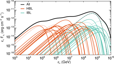
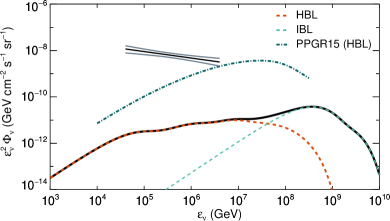
Figure 4: Top panel: All-flavour neutrino energy flux spectra predicted by Scenario A for the sources of our sample with measured $z$ and $\nu_{\rm peak}^{S}$ (thin solid lines). Results for sources with a lower limit on $z$ and $\nu_{\rm peak}^{S}$ are plotted with thin dotted lines. The model prediction for TXS 0506+056 is indicated with a dashed grey line. The total neutrino flux from the sources in the sample is overplotted with a thick black line. A Doppler factor $\delta=10$ and $Y_{\nu\gamma}=0.13$ are assumed for all sources. Bottom panel: Stacked single-flavour neutrino flux predicted in Scenario A (see equation (5)). Dashed coloured lines show the contribution from HBL and IBL objects. The diffuse neutrino flux per flavour from HBL objects for $Y_{\nu\gamma}=0.13$ is also shown (dash-dotted green line; result adapted from Padovani et al. 2015b). The updated best-fit astrophysical muon neutrino flux from IceCube, assuming a single power-law in energy, is overplotted for comparison (solid black line). Solid grey lines indicate the 68 per cent uncertainty range.

Neutrino energy spectra for all sources in the sample with measured $z$ and $\nu_{\rm peak}^{S}$ are presented in Fig. 4 with solid lines (top panel). Dashed lines are used for sources with lower limits on either $z$ or $\nu_{\rm peak}^{S}$, for which equation (4) provides an upper limit on $\varepsilon_{\nu,0}$. Neutrino predictions for HBL and IBL objects are also indicated by different colours. The total neutrino signal from all sources is overplotted with a thick black line. In this scenario, the neutrino spectra of IBL objects peak systematically at higher energies than in HBL. This is a direct result of the dependence of the characteristic neutrino energy on the peak synchrotron frequency (see equation (4)). In case of systematic $\delta$ differences between the IBL and HBL classes the divide in the neutrino spectra from these two blazar classes would be even more pronounced, since $\varepsilon_{\nu,0}\propto\delta^{2}$. These differences would smear out though, if $\delta$ values were instead randomly distributed around a mean value. The predicted neutrino spectrum of TXS 0506+056 (dashed grey line) peaks at $\sim 400$ PeV, well above the 90 per cent confidence level upper limit on the neutrino energy of IC 172209A (IceCube Collaboration, 2018b). This result is in general agreement with SED models of the 2017 multi-messenger flare, where pion production takes place on jet synchrotron photons (e.g. Cerruti et al., 2019). This should be contrasted to models invoking pion production on more energetic photons of external origin, that may yield peak neutrino energies below 1 PeV (e.g. Keivani et al., 2018). Interestingly, the superposition of individual hard ($s<0$) neutrino spectra results in an almost flat neutrino spectrum in $\varepsilon_{\nu}F_{\varepsilon_{\nu}}$ units (thick black line).

On the bottom panel of the same figure we show the stacked muon neutrino and antineutrino flux over the whole sky defined as

$$\varepsilon_{\nu}^{2}\Phi_{\nu_{\mu}+\bar{\nu}_{\mu}}(\varepsilon_{\nu})=\frac{1}{3}\frac{f_{\rm cor}}{4\pi}\sum_{i=1}^{N=39}\varepsilon_{\nu}F_{\varepsilon_{\nu},i},$$ (5)

where we assumed vacuum neutrino mixing and used 1/3 to convert the all-flavour to muon neutrino flux. Here, $f_{\rm cor}=16/47$ accounts for the fact that not all sources selected initially by G20 were plausible neutrino emitters. Dashed coloured lines show the contribution of HBL and IBL objects to the stacked signal. Our estimate is compared to the latest IceCube measurements of the astrophysical diffuse neutrino flux adopted from Stettner (2019) (black and grey lines). The predicted stacked signal is below the diffuse flux measurement by a factor of $\sim 100$, which can be understood as follows. First, the adopted value for $Y_{\nu\gamma}$ ensures that the diffuse flux from the HBL population is in agreement with IceCube upper limits above 10 PeV (Aartsen et al., 2016). Second, our sample contains only a fraction of the whole HBL population. This becomes clearer if we compare the stacked signal from our HBL sub-sample with the predicted diffuse neutrino flux of the HBL population (dash-dotted green line). This has been computed by Padovani et al. (2015b) with Monte Carlo simulations of the blazar population, assuming a universal value of $Y_{\nu\gamma}=0.8$, which has been since then constrained to $0.13$ (Aartsen et al., 2016). Hence, the curve displayed in the figure is scaled down by a factor of $0.8/0.13$ compared to the original one in Padovani et al. (2015b). The stacked signal from the HBL objects of our sample has a spectral shape similar to the diffuse spectrum but with the contribution of individual sources being more prominent because of the small size of the sample.

In summary, if Scenario A is the true physical model for blazar neutrino emission, then the sources identified in our sample are just representative of the whole HBL/IBL blazar population (see also Section 7.4), with masquerading BL Lacs not being “special” sources in terms of neutrino production.

6.2 Scenario B

In this scenario the photon targets for neutrino production through photomeson interactions with the relativistic protons in the jet are provided by the BLR. Hence, this scenario is relevant only to the one FSRQ and the 26 sources with an estimate of (or an upper limit on) $L_{\rm BLR}$ in our sample, which include all but one masquerading BL Lacs.

The BLR photon field has a luminosity that is a fraction $f_{\rm cov}$ of the disk luminosity $L_{\rm d}$, namely $L_{\rm BLR}=0.1\,f_{\rm cov,-1}L_{\rm d}$. We assume that the BLR is a thin spherical shell of characteristic radius $R_{\rm BLR}\simeq 10^{17}\,f_{\rm cov,-1}^{-1/2}L_{\rm BLR,44}^{1/2}$ cm (Ghisellini & Tavecchio, 2008). Here, we introduced the notation $q_{x}=q/10^{x}$ in cgs units, unless otherwise stated. We also assume that the neutrino production region is spherical with comoving radius $R$ and located at distance $r\lesssim R_{\rm BLR}\approx R/\theta_{\rm j}\approx\Gamma\,R$ along a conical jet with bulk Lorentz factor $\Gamma$ and half-opening angle $\theta_{\rm j}$. The accelerated proton distribution is taken to be a power law with slope $p=2$, so that the proton luminosity per logarithmic energy is given by $\varepsilon_{\rm p}L_{\varepsilon_{\rm p}}=L_{\rm p}\mathcal{R}$ with $\mathcal{R}\equiv\ln^{-1}\left(\varepsilon_{\rm p,\max}/\varepsilon_{\rm p,\min}\right)$. For simplicity, we assume that the proton distribution extends from a minimum energy equal to the proton rest mass energy, $\varepsilon_{\rm p,\min}=\Gamma m_{\rm p}c^{2}$, to a maximum energy defined by the Hillas confinement criterion (Hillas, 1984),

$$\varepsilon_{\rm p,\max}=\Gamma eBR\approx eBR_{\rm BLR}\simeq 15\,B_{-0.3}\,f_{\rm cov,-1}^{-1/2}L_{\rm BLR,44}^{1/2}~{}{\rm EeV},$$ (6)

where $e$ is the proton charge and $B$ is the magnetic field strength in the comoving frame. Photohadronic energy losses lead to similar maximum proton energies, if the acceleration process is fast (see e.g. Table II in Murase, Inoue, & Dermer, 2014).

The all-flavour neutrino and antineutrino flux (differential in energy) can be written as (e.g. Murase, Inoue, & Dermer, 2014)

$$\varepsilon_{\nu}F_{\varepsilon_{\nu}}\approx\frac{3}{8}f_{\rm p\pi}\xi F_{\gamma}\mathcal{R}\begin{cases}\left(\frac{\varepsilon_{\nu}}{\varepsilon_{\nu,\rm br}}\right)^{2},&\varepsilon_{\nu}\lesssim\varepsilon_{\nu,\rm br}\\ \left(\frac{\varepsilon_{\nu}}{\varepsilon_{\nu,\rm br}}\right)^{0},&\varepsilon_{\nu,\rm br}\lesssim\varepsilon_{\nu}\lesssim 0.05\,\varepsilon_{\rm p,\max}\end{cases}$$ (7)

where $\xi=L_{\rm p}/L_{\gamma}$ is the baryon loading factor and $\varepsilon_{\nu,\rm br}\approx 0.05\,m_{\rm p}c^{2}\epsilon_{\Delta}/(2\tilde{\varepsilon}_{\rm BLR}(1+z))$ is the typical neutrino energy from pion-production through the $\Delta$ resonance on BLR photons with energy $\tilde{\varepsilon}_{\rm BLR}=10.2$ eV; the latter is measured in the AGN rest frame. Contrary to Scenario A, the photomeson production efficiency is independent of the Doppler factor; it only depends on measurable properties of the BLR, i.e. $f_{\rm p\pi}\approx\tilde{n}_{\rm BLR}\hat{\sigma}_{\rm p\pi}R_{\rm BLR}\approx L_{\rm BLR}\hat{\sigma}_{\rm p\pi}/(4\pi cR_{\rm BLR}\tilde{\varepsilon}_{\rm BLR})$, where $\tilde{n}_{\rm BLR}$ is the number density of BLR photons in the AGN rest frame. The effective cross section is approximated as $\hat{\sigma}_{\rm p\pi}\approx\kappa_{\Delta}\sigma_{\Delta}\delta\epsilon_{\Delta}/\epsilon_{\Delta}$, where $\kappa_{\Delta}\simeq 0.2$ and $\sigma_{\Delta}\simeq 5\times 10^{-28}$ cm² are respectively the inelasticity and cross section of the interaction at the $\Delta$ resonance, $\delta\epsilon_{\Delta}\approx 0.2$ GeV and $\epsilon_{\Delta}\approx 0.34$ GeV is the energy of the $\Delta$ resonance in the proton’s rest frame (Dermer & Menon, 2009).

Meanwhile, secondary pairs injected from charged pion decays and photon-photon annihilation of pionic $\gamma$-rays radiate their energy via synchrotron at energies $\varepsilon_{\gamma}\approx 528~{}B_{-0.3}(\varepsilon_{\rm p}/10~{}{\rm PeV})^{2}(10/\delta)$ MeV with a luminosity comparable to that of neutrinos, namely $\varepsilon_{\gamma}L_{\varepsilon_{\gamma}}\large|_{\rm p\pi,syn}\approx(5/6)\varepsilon_{\nu}L_{\varepsilon_{\nu}}\approx(5/16)f_{\rm p\pi}\varepsilon_{\rm p}L_{\varepsilon_{\rm p}}$ (Murase, Oikonomou, & Petropoulou, 2018). The latter expression can also be written as $\varepsilon_{\gamma}L_{\varepsilon_{\gamma}}\large|_{\rm p\pi,syn}\approx(5/16)f_{\rm p\pi}\xi L_{\gamma}\mathcal{R}\approx(5/16)f_{\rm p\pi}\xi\varepsilon_{\gamma}L_{\varepsilon_{\gamma}}\left(\mathcal{R}/\mathcal{R}_{\gamma}\right)$, where $\mathcal{R}_{\gamma}\equiv\ln^{-1}\left(300~{}{\rm GeV}/100~{}{\rm MeV}\right)$, assuming a $\gamma$-ray spectrum with photon index 2.

The baryon loading factor is an uncertain physical parameter (e.g. Murase, Inoue, & Dermer, 2014; Petropoulou et al., 2020). We therefore compute the value, $\xi^{\rm IC}_{\max}$, needed to match the IceCube sensitivity for each source, namely $(1/3)\varepsilon_{\nu}F_{\varepsilon_{\nu}}=\varepsilon_{\nu}F_{\varepsilon_{\nu}}\large|^{\rm IC}_{\rm sens}$. The declination-dependent sensitivity is a good approximation for the upper limit neutrino flux from the respective sources, because IceCube’s point source search has not yet detected any signal. The parametrisation of the sensitivity is taken from Aartsen et al. (2020a). Another upper limit on $\xi$ can be set from the requirement that the synchrotron cascade luminosity does not overshoot the observed $\gamma$-ray luminosity, namely $\xi^{\rm casc}_{\rm max}=(16/5)f^{-1}_{\rm p\pi}\left(\mathcal{R}/\mathcal{R}_{\gamma}\right)^{-1}$. Figure 5 shows the upper limits on $\xi$ as a function of $L_{\gamma}$ for 27 sources from our sample with redshift and $L_{\rm BLR}$ measurements (or upper limits) assuming $\delta=10$, $B=0.5$ G and a universal $\varepsilon_{\gamma}^{-2}$ spectrum. The Doppler factor is used only in the estimation of characteristic synchrotron photon energy $\varepsilon_{\gamma}$ and does not enter in the calculation of the neutrino fluxes. Except for two sources, the upper limit on $\xi$ set by the electromagnetic cascade constraint is lower than the value required for matching the IceCube sensitivity (i.e. most filled symbols lie below the open symbols). In other words, the neutrino flux needed to exceed the IceCube sensitivity of most sources would be accompanied by an equally bright cascade emission that would exceed the time-integrated Fermi-LAT spectrum. For $\xi=\xi_{\max}^{\rm casc}$ we find $Y_{\nu\gamma}\sim 1$ as expected. In addition to the synchrotron cascade component from photopion interactions that we considered here, synchrotron emission from pairs produced in photopair interactions typically emerges in X-rays (for details, see Murase, Oikonomou, & Petropoulou, 2018). For IBL sources, in particular, where the X-ray flux is lower than the $\gamma$-ray flux in the LAT energy range, the constraint set by the photopair cascade emission is expected to be even stronger than the one derived here.

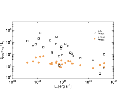
Figure 5: Maximum baryon loading factor as a function of $L_{\gamma}$ for the 27 sources with $L_{\rm BLR}$ measurements (or upper limits). Open symbols show the required $\xi$ to match the IceCube sensitivity for each source assuming a $\varepsilon^{-2}_{\nu}$ spectrum. Filled symbols show the limit on $\xi$ imposed by the electromagnetic cascade (see text for details).

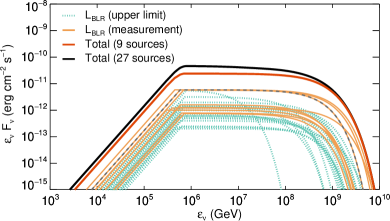
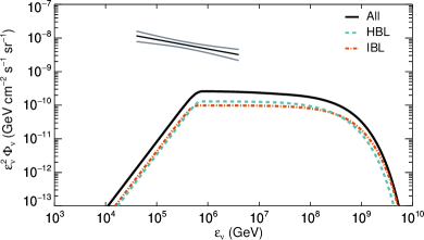
Figure 6: Top panel: All-flavour neutrino energy flux spectra predicted by Scenario B for the 27 sources with measured $L_{\rm BLR}$ (solid lines) or with upper limits on $L_{\rm BLR}$ (dotted lines). The model prediction for TXS 0506+056 is indicated with a dashed grey line. The total neutrino flux from all 27 sources is overplotted with a thick black line. The thick solid red line shows the total neutrino spectrum from 9 sources with measured $L_{\rm BLR}$. Other parameters used are: $\tilde{\varepsilon}_{\rm BLR}=10.2$ eV, $B=0.5$ G, and $\xi=\min(\xi_{\max}^{\rm casc},\xi_{\max}^{\rm IC})$. Bottom panel: Stacked single-flavour neutrino flux predicted in Scenario B using all 27 sources (see equation (5)). Dashed and dash-dotted coloured lines show the contribution from HBL and IBL objects. The updated IceCube best-fit astrophysical muon neutrino flux, assuming a single power-law in energy, is overplotted for comparison (solid black line). Dashed grey lines indicate the 68 per cent uncertainty range.

Using as baryon loading factor the most constraining upper limit, i.e. $\xi=\min(\xi_{\max}^{\rm casc},\xi_{\max}^{\rm IC})$, we compute the individual all-flavour neutrino spectra and the stacked muon neutrino flux using equations (7) and (5), respectively. To make the high-energy cutoff of the neutrino spectrum smoother and given that the proton spectrum is not expected to have a sharp high-energy cutoff, we multiplied the second branch of equation (7) with the term $\exp\left(-20\varepsilon_{\nu}/\varepsilon_{\rm p,max}\right)$. Our results are presented in Fig. 6. In this scenario, the neutrino spectra from individual sources are similar, with the high-energy cutoff being determined by the maximum proton energy (see equation (6)). For 18 out of 27 sources of our sample we could derive only upper limits on $L_{\rm BLR}$ (dotted lines in the top panel). However, the 9 sources with measured $L_{\rm BLR}$ (including TXS 0506+056) make up $\sim 57$ per cent of the total energy-integrated neutrino flux of the sample (compare thick black and red lines). Contrary to Scenario A, there is no specific energy range where HBL or IBL objects dominate the stacked signal, since the target photon field is provided by the BLR and is similar in all sources (compare bottom panels in Figs. 4 and 6). Our stacked single-flavour neutrino signal is lower than the IceCube diffuse flux and extends to EeV energies (see also Murase, Inoue, & Dermer, 2014). The model prediction is still optimistic, since the baryon loading factor might be limited to even lower values than those shown in Fig. 5 by the photopair cascade emission. In fact, if Scenario B, which implies $Y_{\nu\gamma}=1$, were in operation in all IBL/HBL sources, it would contradict the upper limit derived by IceCube on $Y_{\nu\gamma}$ (Aartsen et al., 2016). Therefore, Scenario B should be considered a generous upper limit at work only in a small fraction of sources.

In summary, if Scenario B is the true physical model for blazar neutrino emission, then only a subsample of the HBL/IBL population (with evidence for the presence of external radiation fields) is a neutrino emitter, and no significant differences in the neutrino spectra of HBL and IBL sources are expected.

7 Discussion

7.1 Are our sources different from the rest of the blazar population?

To check if our sources are any different from the rest of the blazar population we would need a large sample of $\gamma$-ray detected BL Lacs with $\nu_{\rm peak}^{S}$ $>10^{14}$ Hz, i.e. IBLs plus HBLs, which unfortunately does not exist. Chang et al. (2019) have put together the largest sample of HBLs, the 3HSP, which includes more than 2,000 sources, 88 per cent of which have a redshift estimation. To make up for the missing IBLs we have compiled a sample of $\gamma$-ray selected objects of this type by accurately verifying $\nu_{\rm peak}^{S}$ for all the sources classified as IBLs (or HBLs and not included in the 3HSP sample) in the Fermi 4LAC catalogue (Ajello et al., 2020). To obtain a sample that is accurate and has a high level of completeness, we have assembled the SED of each candidate located at Galactic latitudes $|b_{\rm II}|>30^{\circ}$ combining the multi-frequency information provided by the latest version of the VOU-Blazar tool (V1.92, Chang, Brandt, & Giommi, 2020), which provides access to data from 67 multi-frequency catalogues and spectral databases, the data retrieved using the SSDC SED tool, and the results of a recent analysis of Swift-XRT data carried out in the framework of the Open Universe initiative (Giommi et al., 2019). Sources with $\nu_{\rm peak}^{S}$ between $10^{14}$ and $10^{15}$ Hz were selected by visual inspection of the available SED data. The final IBL sample includes 183 sources, of which 73 have redshift. By adding the 600 HBLs with $|b_{\rm II}|>30^{\circ}$, we obtain an IBL plus HBL control sample of 783 objects, 630 of which have redshift, detected at the 100 and 97 per cent level in the $\gamma$-ray and radio bands, respectively.

The location of these objects in the $L_{\gamma}-P_{\rm 1.4GHz}$ plane is shown in Fig. 2, where they appear to populate the same region as our sample. This is confirmed by a variety of statistical tests: the two samples have similar mean radio and $\gamma$-ray powers and distributions. Moreover, the control sample displays a very strong linear correlation between the two powers, significant at the $>99.99$ per cent level (and not due to the common redshift dependence) with $L_{\gamma}\propto P_{\rm 1.4GHz}^{0.83\pm 0.04}$, consistent with the correlation found for our sample ($L_{\gamma}\propto P_{\rm 1.4GHz}^{1.04\pm 0.13}$).

As for the $\nu_{\rm peak}^{S}$ – $L_{\gamma}$ plane, Fig. 3 shows that the IBL plus HBL control sources, as was the case for Fig. 2, appear to populate the same region as our sample. Again, this is confirmed by a variety of statistical tests: the two samples have similar mean $\nu_{\rm peak}^{S}$  and distributions. Here we have included the sources without redshift in the IBL sample to increase the statistics (the issue for $L_{\gamma}$ has been discussed above) and excluded the FSRQ from our sample (M87 is already excluded since its $\nu_{\rm peak}^{S}$ is hard to determine, see Section 2). Actually, being $\sim 17$ times larger, the control sample shows that many blazars reach well into the blazar sequence forbidden zone ($L_{\gamma}>10^{45}$ erg s^-1 and $\nu_{\rm peak}^{S}$ $>10^{13}$ Hz).

We find a fraction of extreme sources in our HBL sub-sample of $0.25^{+0.18}_{-0.11}$ (6/24 or $0.29^{+0.19}_{-0.12}$ [where the uncertainties are derived using Poisson statistics] for 7/24, where we have included the source which is very close to being extreme, as discussed in Section 4.3), to be compared with the 3HSP sample (Chang et al., 2019) value of $0.11^{+0.01}_{-0.01}$. While nominally this is a factor $2.5-3$ lower, the two values are still consistent within our (large) uncertainties.

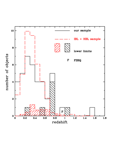
Figure 7: The redshift distribution for our sample (black solid line), with lower limits (denoted by the dashed areas); nine sources are still without redshift. The FSRQ is denoted by an “F”. The red long-dashed line indicates the control sample of IBLs and HBLs scaled to the size of of our sample.

We also compared the redshift distribution, $N(z)$, of our sources (excluding M87 and the FSRQ), to that of the control sample, as shown in Fig. 7 (black solid and red long-dashed line respectively). To take into account the redshift lower limits we used ASURV (Lavalley, Isobe, & Feigelson, 1992), the Survival Analysis package, which employs the routines described in Feigelson & Nelson (1985) and Isobe et al. (1986), which evaluate mean values by dealing properly with limits and also compute the probability that two samples are drawn from the same parent population. The mean redshift is $\langle z\rangle=0.54\pm 0.09$ and $\langle z\rangle=0.37\pm 0.01$ for our sample and the control sample respectively, different at the $\sim 79$ per cent level according to ASURV. The control sample is missing $\sim 20$ per cent of the redshifts, while we have looked very carefully for even weak features and obtained a redshift or a lower limit for all the sources we took a spectrum of. Therefore, the fact that the control sample mean redshift is slightly lower than ours is to be expected. This is confirmed by comparing the newly determined redshifts in Paper I with the corresponding values in the Chang et al. (2019)’s sample (for sources with a previous redshift estimate). Out of seven sources in only one case (3HSP J125848.0$-$04474 a.k.a. 4FGL J1258.7$-$0452, for which our redshift is very well determined [see Fig. 1 of Paper I], which means the previous value from the NASA/IPAC Extragalactic Database was incorrect) is the 3HSP redshift larger than ours, while for the remaining sources our redshifts are typically higher by 0.1 and up to $\gtrsim 0.2$.

7.2 What is the fraction of masquerading BL Lacs?

We find nine masquerading BL Lacs (Table 1, boldface, and Table 2) and eight sources which fulfil none of our criteria and therefore we consider “bona fide” non-masquerading objects (Table 1, italics). For twenty-one sources, however, we do not have the relevant information to make a decision (nine more sources still have no redshift information). Therefore, the fraction of masquerading BL Lacs is in the range $24-79$ per cent but should be well above the lower bound given our conservative selection (Section 4.1). Note that if we include the four extra sources, all of them masquerading, we obtain a higher fraction in the $31-81$ per cent range. We stress that a comparison with other samples is impossible, as nobody has done the characterisation we have done here before.

Giommi, Padovani, & Polenta (2013), by simulating the blazar population in the Fermi 2LAC catalogue (Ackermann et al., 2011b), have found a 70 per cent fraction of masquerading BL Lacs. We note, as they did, that their result is sample and flux limit dependent. The latest Fermi catalogues reach fainter $\gamma$-ray fluxes so one would expect this fraction to decrease, as we reach less luminous, more LEG-like sources. Our value ($>24$ and $\lesssim 80$ per cent) is, therefore, consistent with the simulation results.

A word of caution is in order: if masquerading BL Lacs turn out to be stronger neutrino emitters than other blazars, the fraction we derive here is going to be biased on the high side, given our built-in IceCube selection.

7.3 Do masquerading BL Lacs have different properties from non-masquerading ones?

All sources in our sample with $L_{\gamma}\gtrsim 10^{46}$ erg s^-1 in Fig. 2 are masquerading BL Lacs, as are all objects with $P_{\rm 1.4GHz}\gtrsim 10^{25.5}$ W Hz^-1 (with the exception of 5BZB J1322+3216, for reasons discussed in Section 4.2). More generally, it appears that masquerading BL Lacs tend to be more powerful than non-masquerading ones. This is confirmed for the radio band, where radio powers are $\sim 10$ times larger and for which a Kolmogorov-Smirnov (KS) shows that the two samples are significantly different ($P\sim 99.8$ per cent). A similar result ($P\sim 99.2$ per cent) is obtained using ASURV. Restricting the comparison only to the eight “bona fide” non-masquerading BL Lacs (excluding 5BZB J1322+3216, for reasons discussed above) we obtain practically the same result ($P\sim 98.3$ per cent). It could be argued that a high $P_{\rm 1.4GHz}$ was one of the criteria for selecting masquerading BL Lacs but not a single source has been classified as such only on the basis of its radio power. $L_{\gamma}$ is also $\sim 6$ times larger for masquerading BL Lacs but a KS test shows that the two luminosity distributions are not significantly different. The $P_{\rm 1.4GHz}$ difference is not surprising, as discussed by Padovani et al. (2019), as masquerading BL Lacs need to have relatively high powers, besides having $\nu_{\rm peak}^{S}$$\gtrsim 10^{14}$ Hz, to be able to dilute the quasar-like emission lines, and the radio band is closer to the optical/UV one than the $\gamma$-ray band. Masquerading BL Lacs are also at higher redshift than the rest of the sample but not significantly so ($P\sim 15$ per cent): $\langle z\rangle=0.61\pm 0.19$ vs. $\langle z\rangle=0.40\pm 0.04$, where again we have used ASURV. This is likely to be related to their higher powers.

Fig. 3 suggests that $\nu_{\rm peak}^{S}$ might be smaller for masquerading BL Lacs. Using ASURV, given the two lower limits on this parameter plus the redshift lower limits, which affects also the rest-frame $\nu_{\rm peak}^{S}$, we derive $\langle\log$($\nu_{\rm peak}^{S}$)$\rangle=15.17\pm 0.30$ vs. $\langle\log$($\nu_{\rm peak}^{S}$)$\rangle=16.53\pm 0.27$, with the two distributions being different at the $\sim 98.2$ per cent level. This difference, again, can be explained by a selection effect: the closer $\nu_{\rm peak}^{S}$ is to the band where the lines are diluted, that is the optical–UV band, the more effective the dilution will be and the more likely the source will be a masquerading BL Lac. This is borne out by the $\gamma$-ray simulations mentioned in Section 7.2 (Giommi, Padovani, & Polenta, 2013), which show a steady decrease in the fraction of masquerading BL Lacs as a function of $\nu_{\rm peak}^{S}$, going from $\sim 80$ per cent at $\nu_{\rm peak}^{S}$$\sim 10^{14.5}$ Hz down to less than $\sim 60$ per cent at $\nu_{\rm peak}^{S}$$\sim 10^{17.5}$ Hz.

7.4 Detectability of the theoretically predicted neutrino signal

We now discuss the detectability of the theoretically predicted neutrino signal in Scenarios A and B with IceCube and the interpretation of the observed correlation of neutrinos with our IBL/HBL sample in the context of these two theoretical scenarios.

The number of expected muon and anti-muon neutrinos from a single astrophysical point-like source with persistent neutrino emission at declination $\delta$ in IceCube in the energy range from $\varepsilon_{\nu,{\rm min}}$ to $\varepsilon_{\nu,{\rm max}}$ is,

$$N_{\nu+\bar{\nu}}~{}=~{}\int_{\varepsilon_{\nu,{\rm min}}}^{\varepsilon_{\nu,{\rm max}}}{\rm d}\varepsilon_{\nu}A^{\nu+\bar{\nu}}_{\rm eff}(\varepsilon_{\nu},\delta)\frac{F_{\varepsilon_{\nu}}}{\varepsilon_{\nu}}\Delta\mathrm{T},$$ (8)

where $A^{\nu+\bar{\nu}}_{\rm eff}(\varepsilon_{\nu},\delta)$ is the effective area of the IceCube detector for neutrinos with energy $\varepsilon_{\nu}$, $F_{\varepsilon_{\nu}}$ is the neutrino flux emitted by each modelled source in Scenarios A and B (given by equations 3 and 7 respectively), and $\Delta\mathrm{T}$ is the time interval under consideration.

We estimate the expected number of signal neutrinos from the sources in our sample using equation (8). We remind the reader that the blazar sample studied here is predominantly based on the correlation study of G20. Our goal in this section is to determine whether the neutrino fluxes calculated with Scenarios A and B are consistent with the level of correlation of IBL/HBL blazars with IceCube neutrinos observed by G20.

The neutrinos which were found to correlate with IBLs and HBLs in G20 are a heterogeneous sample from several IceCube analyses with different effective areas which evolve with time. For an estimate, we assume here the effective area of the point-source (PS) analysis (IC86-2012) of Aartsen et al. (2017b) for all neutrinos except the high-energy starting tracks. For these we use instead the high-energy starting muon neutrino effective area published in IceCube Collaboration (2013), as it is as much as a factor of $\sim 10$ smaller than the PS effective area at some declinations. The effective areas of other analyses are not publicly available for arbitrary declinations, but can be as much as a factor of four smaller than the PS effective area (see e.g. Aartsen et al., 2017a).

For our estimate with equation (8) we assume $\varepsilon_{\nu,{\rm min}}=100$ TeV, as beyond this energy the number of atmospheric background neutrinos for declinations $\delta>0^{\circ}$ can be safely neglected. We have tested our sensitivity calculation by comparing it to the IceCube PS sensitivity published in Aartsen et al. (2020a) for an $\varepsilon_{\nu}^{-2}$ neutrino spectrum. We have very good agreement (better than $30$ per cent) in the declination range $0^{\circ}-35^{\circ}$. Outside this range our approximate treatment differs from the IceCube official one by up to a factor of three. However, only three of the studied sources, which were analysed assuming the PS effective area, lie outside the declination range $0^{\circ}-35^{\circ}$.

For the 39 sources modelled under Scenario A, and assuming neutrino emission with $100$ per cent duty cycle over the course of $\sim 10$ years spanned by the neutrino sample, i.e. setting $\Delta\mathrm{T}=10$ yr in equation (8) and assuming $Y_{\nu\gamma}=0.13$, i.e. equal to the upper limit derived by Aartsen et al. (2016), we find that the number of muon neutrinos expected in this model is

$$\sum_{i=1}^{39}N_{\nu+\bar{\nu}}(\varepsilon_{\nu}>100~{}\rm TeV)\sim 0.5.$$ (9)

If all sources from the underlying population of neutrino producing IBLs and HBLs emit neutrinos at a rate proportional to $F_{\gamma}$, we expect the number of neutrinos generated by the IBLs and HBLs found to correlate with the IceCube events by G20 to be

$$\sum_{i=1}^{39}N_{\nu+\bar{\nu},i}\sim\frac{\sum^{39}_{i=1}F_{\gamma,i}}{\sum^{N_{\rm tested~{}sources}}_{i=1}F_{\gamma,i}}\times N_{\rm signal~{}neutrinos}.$$ (10)

Here, 39 is the number of modelled sources, $N_{\rm signal~{}neutrinos}=16\pm 4$ is the number of signal neutrinos, and $N_{\rm tested~{}sources}$ is the total number of IBLs/HBLs in the tested blazar sample. The latter is the number of IBLs and HBLs in the Fermi-4FGL-DR2 catalogue in the area of the sky where the search for matches with IceCube neutrinos was performed by G20 ($|{b}|>10^{\circ}$ and roughly $|\delta|<+35^{\circ}$), which is 769 (536 HBLs and 233 IBLs).

Using $N_{\rm tested~{}sources}=769$ in equation (10) we then obtain $\Sigma_{i=1}^{39}N_{\nu+\bar{\nu},i}\sim 0.6\pm 0.2$, consistent with the number of neutrinos predicted by Scenario A for the 39 modelled sources with equation (9). It is interesting to note that the 39 sources in our sample constitute $39/769\sim 5$ per cent of the population by number and $4$ per cent of the total $F_{\gamma}$. Thus they appear to be an unbiased sample of the underlying ISP/HSP distribution in terms of $F_{\gamma}$.

The nine confirmed masquerading BL Lacs in our sample (see Table 2) are responsible for $\sim 60$ per cent of the total $F_{\gamma}$ in the sample of 39. The eight bona-fide non-masquerading sources produce $\sim 10$ per cent of the total flux, while the twenty-one sources which we cannot classify make the remaining 30 per cent. However, the nine masquerading BL Lacs produce 25 per cent of the expected neutrinos in IceCube, which is close to 9/39. This is because the neutrino expectation in IceCube depends not only on $F_{\gamma}$ but also on the declination, peak neutrino energy, and the IceCube analysis with which each neutrino is detected. The neutrino flux fraction carried by the masquerading BL Lacs is of course dependent on our model assumption that the proton luminosity is linearly dependent on the Fermi-LAT $\gamma$-ray flux of each source. Introducing a different relation between neutrino and electromagnetic flux would affect our estimate as shown, for example, by Krauß et al. (2018). Flares and periods of high activity generally lead to enhanced neutrino production, which scales non-linearly with the $\gamma$-ray flux, see e.g. Murase, Inoue, & Dermer (2014); Tavecchio & Ghisellini (2015); Murase, Oikonomou, & Petropoulou (2018).

We also apply the procedure outlined above to the 27 sources for which we have a firm estimate or upper limit on the BLR luminosity assuming Scenario B. In this case, we expect $\sum_{i=1}^{27}N_{\nu+\bar{\nu}}(\varepsilon>100~{}\rm TeV)=23.7$ muon neutrinos. For this sample the signal is dominated by TXS 0506+056 which is responsible for almost half of the neutrinos expected from the entire sample. Considering only the nine sources with a firm BLR luminosity measurement (i.e. excluding the upper limits), we obtain $\sum_{i=1}^{9}N_{\nu+\bar{\nu}}(\varepsilon_{\nu}>100~{}\rm TeV)=18.5$. Note that 8/9 of these objects are of the masquerading type, which shows, as expected, that these sources make up most of the signal.

We conclude that if Scenario A is in operation in IBLs/HBLs in general it can account for the observed level of correlation found by G20. If this is the underlying neutrino emission mechanism, the sources we have identified through correlations are not special, but representative of the underlying neutrino producing IBLs and HBLs. In the future, Scenario A will be tested by IceCube by means of updated estimates (or upper limits) on the $Y_{\nu\gamma}$ parameter. However, if special conditions are in operation among this subsample of blazars, which are counterparts to IceCube neutrinos in the analysis of G20, in the sense that they do not respect the upper limit on $Y_{\nu\gamma}$ derived for the entire population by IceCube, and neutrino emission proceeds at the maximum rate allowed by the upper limit on $\xi$ derived in section 6.2 (i.e., in the limit that all blazar-neutrino correlations found in G20 are due to high-energy neutrino emission from these 27 sources), the entire neutrino signal of $16\pm 4$ neutrinos observed in G20 can be accounted for.

We note that Scenario B does not take into account possible additional constraints that can be derived on the maximum neutrino flux from each studied source based, for example, on the cascade emission from pairs produced in photopair interactions, which typically emerges in the X-ray energy range in IBLs. For example, for the flaring SED of TXS 0506+056 in 2017, this constraint (see equation 13 of Murase, Oikonomou, & Petropoulou 2018) would result in a stronger upper limit on $\xi$ than $\xi_{\rm max}^{\rm casc}$. Similarly, archival X-ray observations of TXS 0506+056 could limit $\xi$ to a $\sim 10$ times lower value than the one used here (see Fig. 1 of Petropoulou et al., 2020). In other words, what we have studied here with respect to Scenario B is an idealised limit. If the fraction of masquerading BL Lacs and corresponding BLR luminosities of the entire BL Lac population were known we would be able to obtain stronger limits on Scenario B. Additionally, we are aware that if Scenario B is in operation in masquerading BL Lacs then FSRQs might also be strong neutrino emitters and should exhibit a correlation with IceCube neutrinos, which was not observed in the study of G20 nor in previous papers by some of us.

Since FSRQs are almost all of the LBL type, this point is linked to the correlations with LBL rather than IBL/HBL found by some papers both through statistical tests and studies of individual sources. The evidence in this case is less robust or still being debated. For example, Kadler et al. (2016) studied a possible association in space and time between the blazar PKS 1424-418, an LBL at $z=1.522$, and a $\sim$ 2 PeV IceCube neutrino. The positional uncertainty (15.9^∘, 50 per cent radius) of this event, however, is large and the a-posteriori probability of a chance coincidence was estimated to be only about 5 per cent. Hovatta et al. (2021) found associations between radio-flaring blazars mostly of the LBL type and 16 IceCube events but only at the $2\,\sigma$ level. Plavin et al. (2020) cross-correlated a very long baseline interferometry (VLBI) flux density-limited AGN sample with ICeCube events with energies $>200$ TeV. They found that AGN positionally associated with IceCube events have parsec-scale cores stronger than the rest of the sample at the 0.2 per cent (post-trial; i.e. $\sim 2.9\,\sigma$) level. The four brightest AGN, which they selected as highly probable associations, were 3C 279, NRAO 530, PKS 1741$-$038, and OR 103, all blazars of the LBL type. Plavin et al. (2021) further correlated the same VLBI sample with all public IceCube data covering seven years of observations, finding a $3.0\,\sigma$ significance. Combined with their previous result this leads to a post-trial significance of $4.1\,\sigma$. These results are under discussion in the literature (Zhou, Kamionkowski, & Liang, 2021; Desai, Vandenbroucke, & Pizzuto, 2021). Moreover, a comparison between the Plavin et al. (2020) and the G20’s results is not straightforward because of various factors, including: 1. somewhat different IceCube samples; 2. different statistical analysis; 3. different source samples. The latter point is worth elaborating upon. On the one hand, most IBLs/HBLs in the G20’s list have low radio flux densities and therefore cannot belong by construction to the VLBI sample used by Plavin et al. On the other hand, strong radio sources are not excluded by the selection criteria of G20 and moreover all four LBLs selected by Plavin et al. are strong Fermi sources. However, only one of them (PKS 1741$-$038, a.k.a. 5BZQ J1743$-$0350) was matched to IceCube events by G20. NRAO 530, in fact, is located in the error region of a track that is in the Galactic plane ($|b_{\rm II}|<10^{\circ}$), while the other two are outside even the IceCube error ellipses scaled by a factor of 1.5. Finally, 3C 279, despite being the brightest radio and $\gamma$-ray source and the only one of these blazars included in the list of objects used for the search point sources in the 10-year IceCube data set, is not listed among the objects considered as likely neutrino emitters (Aartsen et al., 2020a).

We will address the topic of possible differences in the neutrino emission of FSRQs and masquerading BL Lacs in a forthcoming publication.

In conclusion, Scenario A roughly corresponds to having a neutrino signal from the entire IBL and HBL population, whereas Scenario B corresponds to having a sub-sample of sources which are individually very bright neutrino point sources. At the moment, both are viable to explain the correlation signal observed by G20 and we cannot definitively distinguish between the two. If Scenario A or another mechanism with similar neutrino emission is in operation in IBLs and HBLs, we expect IceCube and other neutrino telescopes to detect neutrinos in the $>$ PeV energy range from the direction of these sources in the future. If, on the contrary, no significant flux of $>$ PeV neutrinos is detected, and a much stronger limit on $Y_{\nu\gamma}$ is obtained with future analyses sensitive in the $>$ PeV energy range, Scenario A will start to be constrained. In other words, if the true value of $Y_{\nu\gamma}$ is $\ll 0.13$, Scenario A would not produce sufficient neutrinos to explain the observed neutrino-IBL/HBL correlation. If the correlation signal grows with future datasets, but the limit on $Y_{\nu\gamma}$ becomes stronger, it would suggest that a fraction of the IBLs and HBLs (for example the masquerading BL Lacs) produce neutrinos at a rate larger than the rest of the population.

8 Conclusions

G20 had selected a unique sample of IBLs and HBLs, $34\pm 9$ per cent of which should be associated with individual IceCube tracks. In Paper I we have presented optical spectroscopy of a large fraction of these sources, which, in combination with already published spectra, has allowed us to determine the redshift, or at least a lower limit to it, for 36 $\gamma$-ray emitting blazars. To these we have added two more sources for which the redshift estimate was photometric and M87 and 3HSP J095507.9+35510, the latter an extreme blazar associated with an IceCube track, which was announced after the G20 paper was completed. Four other extra $\gamma$-ray emitting blazars from a preliminary version of G20’s list were also included.

Here we have carefully characterised these sources to determine their real nature, extending the work done by Padovani et al. (2019) for TXS 0506+056 to a much larger sample of possible neutrino sources. Our main goals were to: (1) quantify the presence of masquerading BL Lacs, i.e., FSRQs in disguise whose emission lines are swamped by a very strong jet, as is the case for TXS 0506+056; (2) check if these sources were any different from the rest of the blazar population; (3) perform a preliminary theoretical analysis of our sample. To this aim we have assembled a set of ancillary data and have also measured and estimated, in many cases for the first time, [O ii] 3727 Å and [O iii] 5007 Å, and $M_{\rm BH}$, respectively.

Source characterisation was based on $L_{\rm[\text{O\,{ii}}]}$ and $L_{\rm[\text{O\,{iii}}]}$, $P_{\rm 1.4GHz}$, $L/L_{\rm Edd}$, and $L_{\gamma}/L_{\rm Edd}$. Also thanks to the very high signal-to-noise ratio of our optical spectra we were able to carry out the first systematic study of masquerading BL Lacs.

Our main conclusions are as follows:

1. we do not find significant evidence for any systematic difference between the sources studied in this paper and other blazars of the same type, i.e. IBLs and HBLs, in terms of their radio and $\gamma$-ray powers, $\nu_{\rm peak}^{S}$, and redshift. This result is based on a large control sample that we selected ex novo. Given that only less than half of our sample is expected to be associated with IceCube tracks, it might also be that the lack of such difference is due to our relatively small sample;

2. the fraction of masquerading BL Lacs in our sample is $>$ 24 per cent and possibly as high as 80 per cent. Although nobody else has derived this value before, this fraction is consistent with the simulation of a $\gamma$-ray selected blazar sample carried out by Giommi, Padovani, & Polenta (2013) and also with a scenario where all the signal found by G20 ($\sim 34$ per cent) comes exclusively from masquerading BL Lacs;

3. masquerading BL Lacs turn out to be exactly as expected: more powerful than the rest in the radio and $\gamma$-ray band, with a slightly smaller $\nu_{\rm peak}^{S}$. These are the properties, which allow them to effectively dilute their strong, FSRQ-like emission lines. Moreover, many of them are outliers of the so-called blazar sequence, in the sense that they have too large of a $\nu_{\rm peak}^{S}$ for their $\gamma$-ray power;

4. MG3 J225517+2409, one of our extra sources, reported to be (weakly) associated with ANTARES and IceCube neutrinos, is also a masquerading BL Lac;

5. we have estimated upper limits on the neutrino emission under two hypotheses about the target photons for the high-energy protons: (1) photons from the jet (Scenario A); (2) photons from the BLR (when the BLR power could be estimated; Scenario B). At present both scenarios are consistent with the observed level of the blazar-neutrino correlation derived by G20. However, in Scenario A our sample is representative of the underlying IBL/HBL population, whereas in Scenario B the sources investigated are stronger neutrino emitters than the rest and might account for the observed blazar-neutrino correlation signal alone. Both scenarios are testable in the near term with IceCube and future neutrino telescopes, placing a more robust upper limit on the normalisation of Scenario A, while we plan to test Scenario B through a detailed study and systematic modelling of the individual photon-neutrino SEDs, which will be the next phase of this project.

Data Availability

The flux-calibrated and dereddened spectra are available in the online database ZBLLAC.

Appendix A Host galaxies and black hole mass

For eighteen objects with known redshift and a signature of the host galaxy in their optical spectra we performed a decomposition of the optical spectra as the sum of a power law and an elliptical galaxy template (Mannucci et al., 2001) following the method described in Section 3.2.3 and Paper I. Our results are given in Table LABEL:tab:apdx while some examples of the spectral decomposition using SDSS spectra are given in Figure 8; for other cases see Paiano et al. (2021). In five further cases the spectrum was not available in electronic format or was not flux calibrated. Therefore, we measured the host galaxy magnitude directly from an $r$ band image.

$M_{\rm BH}$ was then evaluated. The dispersion on the $M_{\rm BH}-M(R)$ relationship is $\sim 0.45$ dex (Labita et al., 2007) and we combined this uncertainty with the error on the host galaxy magnitude. For thirteen of these objects Paliya et al. (2021) have derived independently $M_{\rm BH}$ based on measurements of the stellar velocity dispersion, $\sigma$, and the $M_{\rm BH}-\sigma$ relationship (Gültekin et al., 2009) that was first applied to BL Lacs by Falomo, Kotilainen, & Treves (2002) and Barth, Ho, & Sargent (2002). For ten of them the two $M_{\rm BH}$ estimates are in reasonable agreement, with a difference $\lesssim$ 0.5 dex. For three sources, however, (3HSP 023248.5+20171, 3HSP J094620.2+01045, 3HSP J180849.7+35204), a significant difference ($>$ 1 dex) was found. The case of 3HSP J094620.2+01045 is explained by the different redshift (0.128 vs. 0.576) used by Paliya et al. (2021); the latter value is the SDSS one and is confirmed by a careful inspection of the spectrum. In the case of 3HSP 023248.5+20171 Paliya et al. (2021) report log$(M_{\rm BH}/M_{\odot})=10.8$ based on the measurement of $\sigma$ from a paper copy of the spectrum published by Perlman et al. (1996) that is dominated by the contribution of the host galaxy. The SDSS magnitude of this object is r = 16.2. Assuming that the whole flux is from the host galaxy the absolute magnitude is $M(R)=-22.9$ that implies log($M_{\rm BH}/M_{\odot})=8.8$. Finally, for 3HSP J180849.7+35204 again Paliya et al. (2021) used a spectrum obtained by Peña-Herazo et al. (2019) to obtain log($M_{\rm BH}/M_{\odot})=9.36$ based on $\sigma$, while using the same spectrum (available in ZBLLAC) and our spectral decomposition we obtained log($M_{\rm BH}/M_{\odot})=8.0$. This difference is inconsistent with the dispersion of the two $M_{\rm BH}-\sigma$ and $M_{\rm BH}-M(R)$ relationships.

Table 5: Measurement of host galaxy luminosity and black hole mass

Name	$z$	$M(R)$	N/H	log$(M_{\rm BH}/M_{\odot}$)	Method	Reference
3HSP J010326.0+15262	0.246	$-$22.4	0.5	$8.6\pm 0.4$	SpD	SDSS
5BZU J0158+0101	0.454	$-$20.0	5.0	$7.4\pm 0.6$	SpD	ZBLLAC
3HSP 023248.5+20171	0.139	$-$22.9	0.0	$8.8\pm 0.4$	ImD	SDSS
3HSP J033913.7$-$17360	0.066	$-$22.5	0.0	$8.6\pm 0.4$	ImD	PanSTARRS
CRATES J052526$-$201054	0.091	$-$21.5	0.3	$8.1\pm 0.4$	SpD	ZBLLAC
3HSP J062753.3$-$15195	0.31	$-$23.2	0.5	$9.0\pm 0.4$	SpD	ZBLLAC
3HSP J085410.1+27542	0.493	$-$23.2	1.8	$9.0\pm 0.4$	SpD	ZBLLAC
3HSP J094620.2+01045	0.576	$-$22.5	5.0	$8.6\pm 0.6$	SpD	SDSS
3HSP J095507.9+355101	0.557	$-$22.9	0.0	$8.8\pm 0.4$	ImD	P20
3HSP J111706.2+20140	0.138	$-$21.4	2.5	$8.1\pm 0.4$	SpD	SDSS
3HSP J123123.1+14212	0.256	$-$22.0	2.5	$8.4\pm 0.4$	SpD	SDSS
3HSP J125821.5+21235	0.627	$-$21.2	5.0	$8.0\pm 0.6$	SpD	ZBLLAC
3HSP J125848.0$-$04474	0.418	$-$22.1	4.5	$8.4\pm 0.5$	SpD	ZBLLAC
5BZB J1322+3216	0.4	$-$21.7	4.0	$8.2\pm 0.5$	SpD	SDSS
VOU J135921$-$115043	0.242	$-$22.3	0.5	$8.6\pm 0.4$	SpD	ZBLLAC
3HSP J140449.6+65543	0.362	$-$21.8	5.0	$8.3\pm 0.6$	SpD	SDSS
VOU J143934$-$252458	0.16	$-$22.3	0.0	$8.5\pm 0.4$	ImD	PanSTARRS
3HSP J143959.4$-$23414	0.309	$-$22.3	2.5	$8.6\pm 0.4$	SpD	ZBLLAC
3HSP J144656.8$-$26565	0.331	$-$22.4	1.5	$8.6\pm 0.4$	SpD	ZBLLAC
3HSP J153311.2+18542	0.307	$-$22.1	2.0	$8.4\pm 0.4$	SpD	SDSS
3HSP J155424.1+20112	0.222	$-$22.5	0.5	$8.6\pm 0.4$	SpD	SDSS
3HSP J180849.7+35204	0.141	$-$21.3	1.5	$8.0\pm 0.4$	SpD	ZBLLAC
3HSP J213314.3+25285	0.294	$-$22.8	0.0	$8.8\pm 0.4$	ImD	PanSTARRS

Notes. Col. 1: name; Col. 2: redshift; Col. 3: absolute magnitude of the host galaxy in the R filter; Col. 4: N/H, i.e. the ratio of the fluxes of the nucleus to the host galaxy at 6000 Å; Col. 5: the logaritmih of $M_{\rm BH}$ in solar units (see text); Col. 6: Method: SpD = Spectrum decomposition; ImD = Image decomposition; Col. 7: reference to the spectrum or the image: P20 (Paiano et al., 2020), SDSS (Ahumada et al., 2020), ZBLLAC (Landoni et al., 2020), PanSTARRS (https://panstarrs.stsci.edu/).

A.1 Notes for individual targets

3HSP J095507.9+355101

The measurement of log($M_{\rm BH}/M_{\odot})=8.8$ for this source is based on the absolute magnitude of the host galaxy from the R band image by Paiano et al. (2020). This value is different from the one previously reported by these authors as that was based on different cosmological parameters.

5BZB J1322+32

We fitted the observed SDSS optical spectrum into a power law (dominant in the blue region) and a galaxy template. An acceptable fit was obtained for $z=0.4$ and a galaxy of $M(R)=-21.7$. From this decomposition log($M_{\rm BH}/M_{\odot})=8.2$ is derived. Note that a redshift value $z=0.396$ is reported in Paliya et al. (2021) based on the measurement of the stellar velocity dispersion from the SDSS spectrum, which is however featureless and which reports a value derived from the automatic SDSS procedure $z=1.4\pm 0.8$.

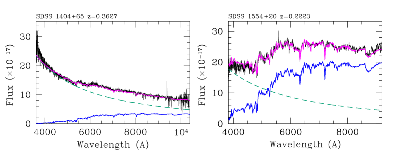
Figure 8: Examples of spectral decomposition for two targets using SDSS spectra. The observed optical spectrum (black line) is fitted by the combination of a power law (green dashed line) plus a template spectrum (blue line) of an elliptical galaxy (see text). The best fit is given by the solid magenta line. Fluxes are in units of erg cm^-2 s^-1 Å^-1.

References

- Aartsen et al. (2016) Aartsen M. G., Abraham K., Ackermann M., Adams J., Aguilar J. A., Ahlers M., Ahrens M., et al., 2016, PhRvL, 117, 241101
- Aartsen et al. (2017a) Aartsen M. G., Ackermann M., Adams J., Aguilar J. A., Ahlers M., Ahrens M., Altmann D., et al., 2017a, APh, 92, 30
- Aartsen et al. (2017b) Aartsen M. G., Abraham K., Ackermann M., Adams J., Aguilar J. A., Ahlers M., Ahrens M., et al., 2017b, ApJ, 835, 151
- Aartsen et al. (2017c) Aartsen M. G., Ackermann M., Adams J., Aguilar J. A., Ahlers M., Ahrens M., Samarai I. A., et al., 2017c, ApJ, 849, 67
- Aartsen et al. (2019) Aartsen M. G., Ackermann M., Adams J., Aguilar J. A., Ahlers M., Ahrens M., Alispach C., et al., 2019, ApJ, 886, 12
- Aartsen et al. (2020a) Aartsen M. G., Ackermann M., Adams J., Aguilar J. A., Ahlers M., Ahrens M., Alispach C., et al., 2020a, PhRvL, 124, 051103
- Aartsen et al. (2020b) Aartsen M. G., Ackermann M., Adams J., Aguilar J. A., Ahlers M., Ahrens M., Alispach C., et al., 2020b, PhRvL, 125, 121104
- Abdo et al. (2010) Abdo A. A., Ackermann M., Ajello M., et al., 2010, ApJ, 716, 30
- Abdollahi et al. (2020) Abdollahi S., Acero F., Ackermann M., Ajello M., Atwood W. B., Axelsson M., Baldini L., et al., 2020, ApJS, 247, 33
- Ackermann et al. (2011a) Ackermann M., Ajello M., Allafort A., Angelakis E., Axelsson M., Baldini L., Ballet J., et al., 2011a, ApJ, 741, 30
- Ackermann et al. (2011b) Ackermann M., Ajello M., Allafort A., Antolini E., Atwood W. B., Axelsson M., Baldini L., et al., 2011b, ApJ, 743, 171
- Ackermann et al. (2015) Ackermann M., et al., 2015, ApJ, 810, 14
- Ahlers & Halzen (2015) Ahlers M., Halzen F., 2015, Rep. Prog. Phys., 78, 126901
- Ahumada et al. (2020) Ahumada R., Prieto C. A., Almeida A., Anders F., Anderson S. F., Andrews B. H., Anguiano B., et al., 2020, ApJS, 249, 3
- Ajello et al. (2020) Ajello M., Angioni R., Axelsson M., Ballet J., Barbiellini G., Bastieri D., Becerra Gonzalez J., et al., 2020, ApJ, 892, 105
- Albert et al. (2021) Albert A., André M., Anghinolfi M., Anton G., Ardid M., Aubert J.-J., Aublin J., et al., 2021, ApJ, 911, 48
- Anchordoqui (2019) Anchordoqui L. A., 2019, PhR, 801, 1
- Atoyan & Dermer (2001) Atoyan A., Dermer C. D., 2001, PhRvL, 87, 221102
- Barth, Ho, & Sargent (2002) Barth A. J., Ho L. C., Sargent W. L. W., 2002, ApJL, 566, L13.
- Ballet et al. (2020) Ballet J., Burnett T. H., Digel S. W., Lott B., The Fermi-LAT Collaboration, 2020, arXiv:2005.11208
- Begelman, Fabian, & Rees (2008) Begelman M. C., Fabian A. C., Rees M. J., 2008, MNRAS, 384, L19
- Biteau et al. (2020) Biteau J., Prandini E., Costamante L., Lemoine M., Padovani P., Pueschel E., Resconi E., et al., 2020, NatAs, 4, 124
- Bressan, Granato, & Silva (1998) Bressan, A., Granato G.L. & Silva L. 1998, A&A, 332, 135
- Celotti & Ghisellini (2008) Celotti A., Ghisellini G., 2008, MNRAS, 385, 283
- Cerruti et al. (2015) Cerruti M., Zech A., Boisson C., Inoue S., 2015, MNRAS, 448, 910
- Cerruti et al. (2019) Cerruti M., Zech A., Boisson C., Emery G., Inoue S., Lenain J.-P., 2019, MNRAS, 483, L12
- Chang et al. (2019) Chang Y.-L., Arsioli B., Giommi P., Padovani P., Brandt C. H., 2019, A&A, 632, A77
- Chang, Brandt, & Giommi (2020) Chang Y.-L., Brandt C., & Giommi P., 2020, Astronomy & Computing, 30, 100350
- Dermer & Menon (2009) Dermer C. D., Menon G., 2009, High Energy Radiation from Black Holes: Gamma Rays, Cosmic Rays, and Neutrinos
- Desai, Vandenbroucke, & Pizzuto (2021) Desai A., Vandenbroucke J., Pizzuto A., for the IceCube collaboration, 2021, PoS, ICRC2021, 949 (arXiv:2107.08115)
- Event Horizon Telescope Collaboration et al. (2019) Event Horizon Telescope Collaboration, Akiyama K., Alberdi A., Alef W., Asada K., Azulay R., Baczko A.-K., et al., 2019, ApJL, 875, L1
- Falomo, Kotilainen, & Treves (2002) Falomo R., Kotilainen J. K., Treves A., 2002, ApJL, 569, L35
- Falomo, Pian, & Treves (2014) Falomo R., Pian E., Treves A., 2014, A&ARv, 22, 73
- Feigelson & Nelson (1985) Feigelson E. D., Nelson P. I. 1985, ApJ, 293, 192
- Fossati et al. (1998) Fossati G., Maraschi L., Celotti A., Comastri A., Ghisellini G., 1998 MNRAS, 299, 433
- Gao, Pohl, & Winter (2017) Gao S., Pohl M., Winter W., 2017, ApJ, 843, 109
- Ghisellini et al. (1998) Ghisellini G., Celotti A., Fossati G., Maraschi L., Comastri A., 1998, MNRAS, 301, 451
- Ghisellini & Tavecchio (2008) Ghisellini G., Tavecchio F., 2008, MNRAS, 387, 1669
- Ghisellini et al. (2011) Ghisellini G., Tavecchio F., Foschini L., Ghirlanda G., 2011, MNRAS, 414, 2674
- Ghisellini et al. (2017) Ghisellini G., Righi C., Costamante L., Tavecchio F., 2017, MNRAS, 469, 255
- Giommi et al. (2012a) Giommi P., Padovani P., Polenta G., Turriziani S., D’Elia V., Piranomonte S., 2012a, MNRAS, 420, 2899
- Giommi et al. (2012b) Giommi P., Polenta G., Lähteenmäki A., Thompson D. J., Capalbi M., Cutini S., Gasparrini D., et al., 2012b, A&A, 541, A160