Uncertainty, Edge, and Reverse-Attention Guided Generative Adversarial Network for Automatic Building Detection in Remotely Sensed Images

Abstract

Despite recent advances in deep-learning based semantic segmentation, automatic building detection from remotely sensed imagery is still a challenging problem owing to large variability in the appearance of buildings across the globe. The errors occur mostly around the boundaries of the building footprints, in shadow areas, and when detecting buildings whose exterior surfaces have reflectivity properties that are very similar to those of the surrounding regions. To overcome these problems, we propose a generative adversarial network based segmentation framework with uncertainty attention unit and refinement module embedded in the generator. The refinement module, composed of edge and reverse attention units, is designed to refine the predicted building map. The edge attention enhances the boundary features to estimate building boundaries with greater precision, and the reverse attention allows the network to explore the features missing in the previously estimated regions. The uncertainty attention unit assists the network in resolving uncertainties in classification. As a measure of the power of our approach, as of December 4, 2021, it ranks at the second place on DeepGlobe’s public leaderboard despite the fact that main focus of our approach — refinement of the building edges — does not align exactly with the metrics used for leaderboard rankings. Our overall F1-score on DeepGlobe’s challenging dataset is 0.745. We also report improvements on the previous-best results for the challenging INRIA Validation Dataset for which our network achieves an overall IoU of 81.28% and an overall accuracy of 97.03%. Along the same lines, for the official INRIA Test Dataset, our network scores 77.86% and 96.41% in overall IoU and accuracy. We have also improved upon the previous best results on two other datasets: For the WHU Building Dataset, our network achieves 92.27% IoU, 96.73% precision, 95.24% recall and 95.98% F1-score. And, finally, for the Massachusetts Buildings Dataset, our network achieves 96.19% relaxed IoU score and 98.03% relaxed F1-score over the previous best scores of 91.55% and 96.78% respectively, and in terms of non-relaxed F1 and IoU scores, our network outperforms the previous best scores by 2.77% and 3.89% respectively.

I Introduction

While a great deal of progress has already been made in the automatic detection of building footprints in aerial and satellite imagery, several challenges still remain. Most of these can be attributed to the high variability in how the buildings show up in such images in different parts of the world, by the effect of shadows on the sensed data, and by the presence of occlusions caused by nearby tall structures and high vegetation. Problems are also caused by the fact that the reflectivity signatures of several types of building materials are close to those for the materials that are commonly used for the construction of roads and parking lots.

With regard to the performance of the deep-learning based methods for discriminating between the buildings and the background, the commonly used metrics used for evaluating the algorithms only ensure that the bulk of the building footprints is extracted. The metrics do not enforce the requirement of contiguity of the pixels that belong to the same building [1, 2, 3, 4, 5, 6]. This has led some researchers to formulate post-processing steps like the Conditional Random Fields (CRFs) [7, 8] during inference for invoking spatial contiguity in the output label maps.

Even more importantly, the semantic-segmentation metrics for identifying the buildings are silent about the quality of the boundaries of the pixel blobs [1, 3, 9, 10, 11, 12]. Since the number of pixels at the perimeter of a convex shape is roughly proportional to the square-root of the pixels in the interior, incorrectly labeling even a tiny fraction of the overall building pixels may correspond to an exaggerated effect on the quality of the boundary.

These problems related to enforcing the spatial contiguity constraint and to ensuring the quality of the building boundaries only become worse in the presence of confounding factors such as shadows, the similarity between the reflectivity properties of the building exteriors and their surroundings, etc.

We address these challenges in a new generative adversarial network (GAN) [13] for segmenting building footprints from high-resolution remotely sensed images. We adopt an adversarial training strategy to enforce long-range spatial label contiguity, without adding any complexity to the trained model during inference. In our adversarial network, the discriminator is designed to correctly distinguish between the predicted labels and the ground-truth labels and is trained by optimizing a multi-scale L1 loss [14]. The generator, an encoder-decoder framework with embedded uncertainty attention and refinement modules, is trained to predict one-channel binary maps with pixel-wise labels for building and non-building classes.

Our network incorporates several novel ideas, such as the Uncertainty Attention Unit that is introduced at each data abstraction level between the concatenation of the encoder feature map with the decoder feature map. This unit focuses on those feature regions where the network has not shown confidence during its previous predictions. That is likely to happen at the boundaries of the building shapes, in shadow areas, and in those regions of an image where the building pixel signatures are too close to the background pixel signatures.

Another novel aspect of our network is the Refinement Module that consists of a Reverse Attention Unit and an Edge Attention Unit. This module is introduced after each stage in the decoder to gradually refine the prediction maps. Starting with the bottleneck layer of the encoder-decoder network and using an Atrous Spatial Pyramid Pooling (ASPP) [3] layer, the network first predicts a coarse prediction map that is rich in semantic information but lacks fine detail (Figure 2). The coarse prediction map is then gradually refined by adding residual predictions obtained from the two attention units in each stage of decoding. The Edge Attention Unit amplifies the boundary features, and, thus, helps the network to learn precise boundaries of the buildings. And the Reverse Attention Unit allows the network to explore the regions that were previously classified as non-building, which enables the network to discover the missing building pixels in the previously estimated results.

In addition to the adversarial loss, we also use deep supervision (shown as thick arrows in Figure 2) in our architecture for efficient back propagation of the gradients through the deep network structure. By deep supervision, we refer to the losses computed for each intermediate prediction map. These losses are added to the final layer’s loss. Deep supervision guides the intermediate prediction maps to become more directly predictive of the final labels. We compute weighted dice loss and shape loss for the final prediction map as well as for each intermediate prediction map.

The power of our approach is best illustrated by its ranking at number 2 in the “DeepGlobe Building Extraction Challenge” at the following website:

https://competitions.codalab.org/competitions/18544#results

In the experimental results that we will report in this paper, the reader will see significant performance improvements over the previous-best results for four different datasets, two of which are known to be challenging (DeepGlobe and INRIA), and two others that are older but very well known in semantic segmentation research (WHU and the Massachusetts Buildings Dataset). While our performance numbers presented in the Results section speak for themselves, the reader may also like to see a visual example of the improvements in the quality of the building prediction maps produced by our framework. Figure 1 shows a typical example. Additionally, our results on the INRIA Aerial Image Labeling Dataset [15] demonstrate that our proposed network can be generalized to detect buildings in different cities across the world without being directly trained on each of them.

The rest of the paper is organized as follows. In Section II, we review current state-of-the-art building segmentation algorithms and explain distinctive features of our proposed algorithm in relation to the past literature. Section III gives a detailed description of our network architecture and its various components. We explain our training strategy and the loss functions used in Section IV. In Section V, we describe the datasets we have used for our experiments. Subsequently, in Section VI, we provide detailed description of our experimental setup. In Section VII, we compare the performance of our approach with other state-of-the-art methods. We conduct a detailed discussion about our results and present an ablation study involving various components of our network in Section VIII. Finally, we conclude and summarize the paper in Section IX.

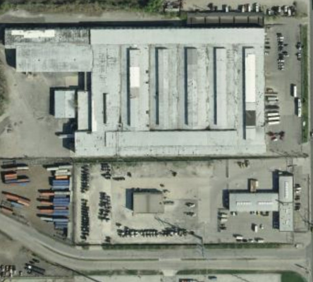
(a) Input Image

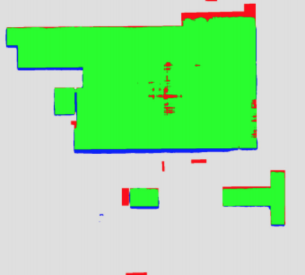
(b) GAN-SCA [11]

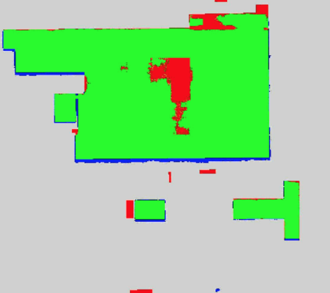
(c) Our baseline network with no attention units

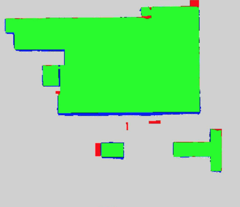
(d) Our network with attention units

Figure 1: Comparing segmentation results using our approach and another state-of-the-art approach (GAN-SCA) on an image patch over Chicago from the INRIA Dataset. Green: True positives ; Blue: False Positives; Red: False negatives, Grey: True negatives.

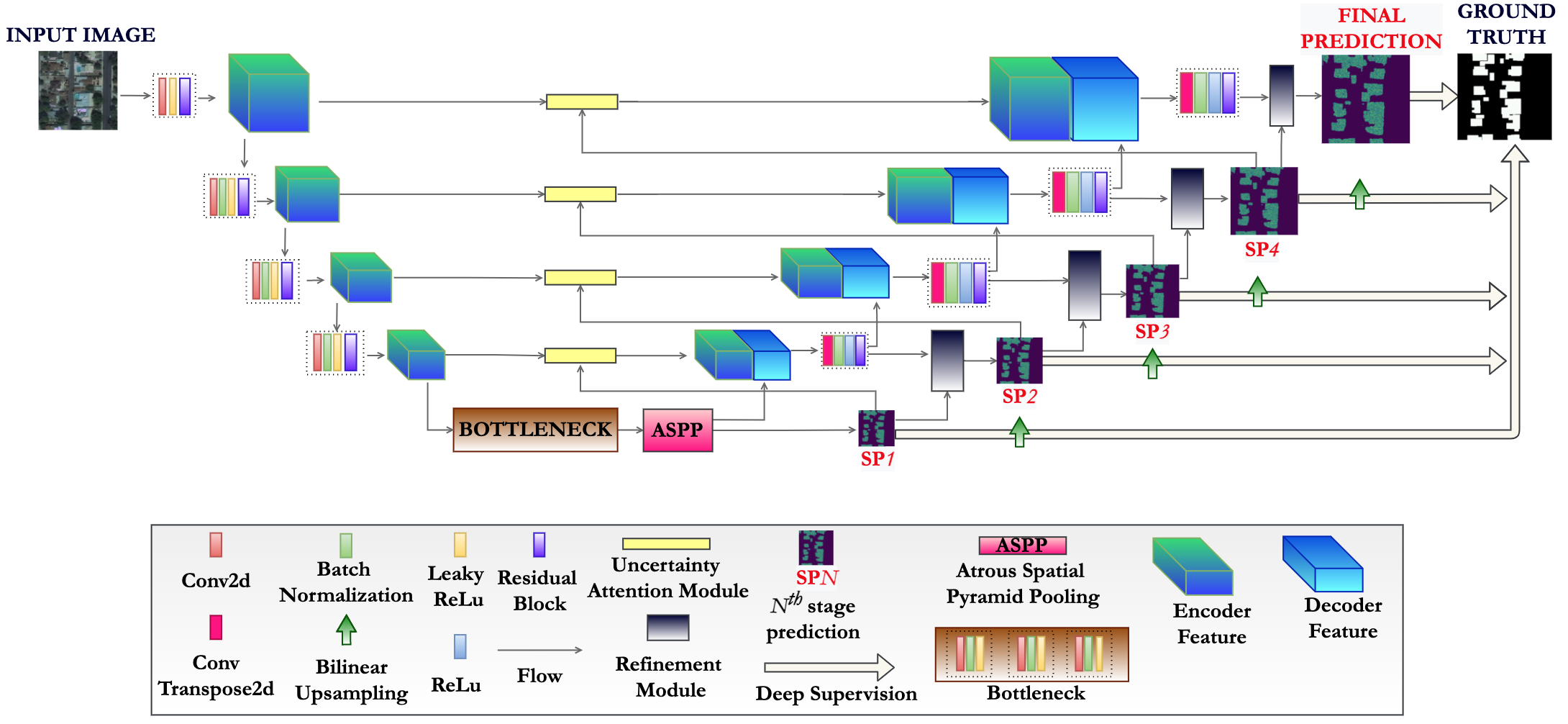
Figure 2: Segmentation Framework

II Related Works

The past decade of research in image segmentation methods has witnessed the deep learning based approaches [16, 17, 18, 9, 19, 20, 21, 22, 23, 24, 25, 26] outperforming the more traditional approaches [27, 28, 29, 30, 31, 32, 33, 34, 35, 36]. Inspired by the success of the deep learning based methods, more recently the researchers have focused on developing neural network based frameworks for detecting building footprints from high-resolution remotely sensed images [37, 38, 39, 5, 40, 41, 42, 43, 44, 45, 46, 47, 48, 49].

Mnih was the first to use a CNN to carry out patch-based segmentation in aerial images [1]. Saito et al. in [2] also used a patch based CNN for road and building detection from aerial images. However, the patch-based methods suffer from the problem of limited receptive fields and large computational overhead, and require post-processing steps [7] to refine the segmentation results. The patch-based approaches were soon surpassed by pixel-based methods [6, 4] that applied state-of-the-art neural network models, like the hierarchical fully convolutional network (FCN) and stacked U-Nets, to perform pixel-wise prediction of building footprints in aerial images. However, these approaches do not fully utilize the structural and contextual information of the ground objects that can help to distinguish the buildings from their heterogeneous backgrounds.

The shortcomings of the current state-of-the-art in deep learning based methods are being addressed by several ongoing research efforts [50, 51, 42, 52, 53, 54, 55, 56]. The work reported in [50] addresses the problems caused by large variations in the building sizes in satellite imagery. On the other hand, the works reported in [51, 52, 53, 57, 58, 59] deal with the preservation of the sharpness of the building boundaries. There are also the works reported in [54, 12] that attempt to detect buildings even when only a part of a building is visible.

In order to leverage large-scale contextual information and extract critical cues for identifying building pixels in the presence of complex background and when there is occlusion, researchers have proposed methods to capture local and long-range spatial dependencies among the ground entities in the aerial scene [55, 56]. Several researchers are also using tranformers [60], attention modules [12, 61, 62, 63] and multi-scale information [43, 45, 8, 46, 64, 65, 66] for this purpose. Recently, multi-view satellite images [67, 68] are also being used to perform semantic segmentation of points on ground.

GANs [13] are also gaining popularity in solving semantic segmentation problems. In GAN-based approaches to building detection [10, 11, 69, 70], the generator is basically a segmentation network that aims to produce building label maps that cannot be distinguished from the ground-truth ones by the discriminator. By training the segmentation and the discriminator networks alternatively, the likelihood associated with the joint distribution of all the labels that are possible at the different pixel locations can be maximized as a whole, which amounts to enforcing long-range spatial dependency among the labels. Using this logic, in [10], Sebastian et al. illustrated how the use of adversarial learning can improve the performance of the existing benchmark semantic segmentation networks [21, 3]. Along roughly the same lines, Li et al. adopted adversarial training in [69] to detect buildings in overhead images where the segmentation network is a fully convolutional DenseNet model and the discriminator an autoencoder. In [70], the authors used a SegNet model with a bidirectional convolutional LSTM as the segmentation network.

The work presented in this paper comes closest to the approach adopted in [11] in which the authors have proposed a GAN with spatial and channel attention mechanisms to detect buildings in high-resolution aerial imagery. In this contribution, the spatial and the channel attention mechanisms are embedded in the segmentation architecture to selectively enhance important features on the basis of their spatial information in the different channels. In contrast with [11], our framework focuses the attention units where they are needed the most — these would be the pixels where the predictions are being made with low probabilities.

Despite the successes of the previous contributions mentioned in this section, the predicted building label maps are still found lacking with regard to the overall quality of building segmentations. At the pixel level, we still have misclassifications at a higher rate at those locations where the classification accuracy is most important — at and in the vicinity of the boundaries of the buildings and where there are shadows and obscurations. Furthermore, the methods that have been proposed to date tend to be locale specific. That is, they do not generalize straightforwardly to the different geographies around the world without further training. In this paper, we aim to overcome these shortcomings with the help of uncertainty and refinement modules that we embed in the segmentation network of our adversarial framework. We show empirically that our model outperforms the state-of-the models on well-known publicly available datasets [1, 15, 54, 71, 72].

III Proposed Architecture

In this section, we describe our proposed attention-enhanced generative adversarial network for detecting building footprints in remotely sensed images. The framework is composed of two parts: an attention-enhanced segmentation network ($\mathcal{S}$) and a critic network ($\mathcal{C}$). Our segmentation network, attention units and critic network are described in details in Sections III-A, III-B and III-C respectively.

III-A Segmentation Network

Our segmentation framework ($\mathcal{S}$), illustrated in Figure 2, is a fully convolutional encoder-decoder network that takes in a 3-channel remotely sensed image and generates a 1-channel prediction map in which each pixel value indicates that pixel’s probability of belonging to the building class.

$\mathcal{S}$ uses four strided convolutional (Conv) layers for encoding the input images. The kernel size is set to 7 for the first two layers and 5 for the next two. The stride is set to 2 in all the layers. The output of the encoder is a feature map at $1/16$-th the spatial resolution of the input images. The number of channels goes up by a factor of 2 in each layer.

The feature maps thus produced at the bottleneck layer of the network are processed by an ASPP module [3] to capture the global contextual information for more accurate pixel-wise predictions. The ASPP module consists of a $1\times 1$ Conv layer, three $3\times 3$ Conv layers with dilation rates of 2, 4, and 6, and a global context layer incorporating average pooling and bilinear interpolation. The resulting feature maps from the five layers of ASPP are concatenated and passed through another $3\times 3$ Conv layer, where they form the output of the ASPP module that is fed directly into the decoder. In addition to that, we pass the feature maps from the ASPP module through a $1\times 1$ Conv layer to produce the top-most prediction map that is low in resolution but rich in semantic information.

The decoder uses kernels with increasingly larger receptive fields (7,9 and 11) in order to enlarge the representational scope of each pixel. Each layer of the decoder uses a transpose convolution (ConvTranspose2d) to up-sample the incoming feature map while halving the number of feature channels.

Residual blocks are added after every downsampling and upsampling layer. Each residual block consists of a $1\times 1$ Conv, followed by a $3\times 3$ Conv and then another $1\times 1$ Conv. Skip connections are used in a similar fashion as that of the U-Net [16] to concatenate the corresponding layers of the encoder and the decoder. As shown by the yellow boxes in Figure 2, an Uncertainty Attention Module is used for this concatenation at each abstraction level in network. This allows the network to focus on the features in those regions where the network has not shown confidence in the predictions made at the lower abstraction level. Detailed description of this module is presented in Section III-B2.

Batch normalization is used after each convolutional layer except the first layer of the encoder. After each batch normalization, Leaky ReLU with a leak slope of 0.2 is used in all downsampling blocks, and a regular ReLU has been used for all the upsampling layers.

We also apply a Refinement Module consisting of a Reverse Attention Unit and an Edge Attention Unit in each stage of the decoder. This module is used to learn residual predictions after every stage of decoding and gradually refine the prediction map estimated in the previous stage until the final prediction map is obtained. Details of this module are provided in Section III-B1.

III-B Attention in Segmentation Network

III-B1 Refinement Module

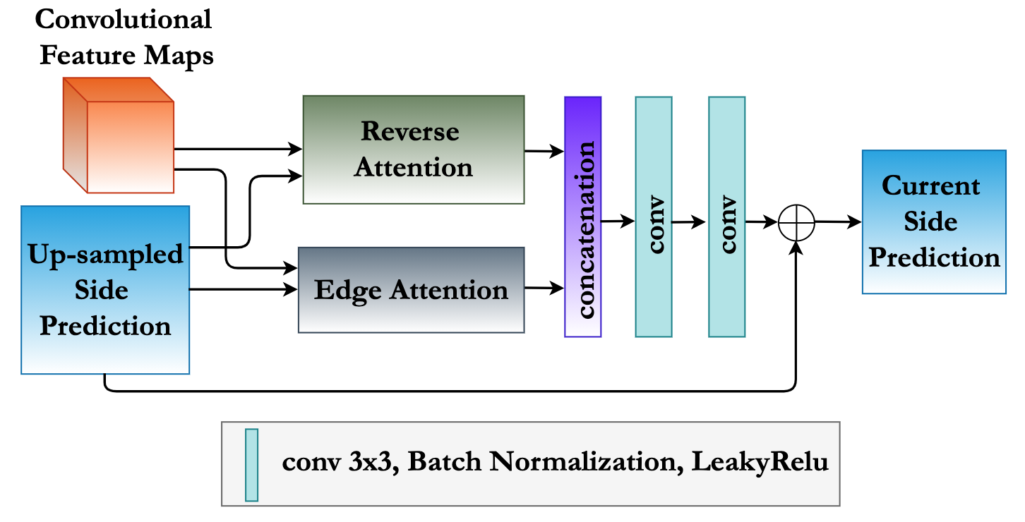
Figure 3: Refinement Module (RM)

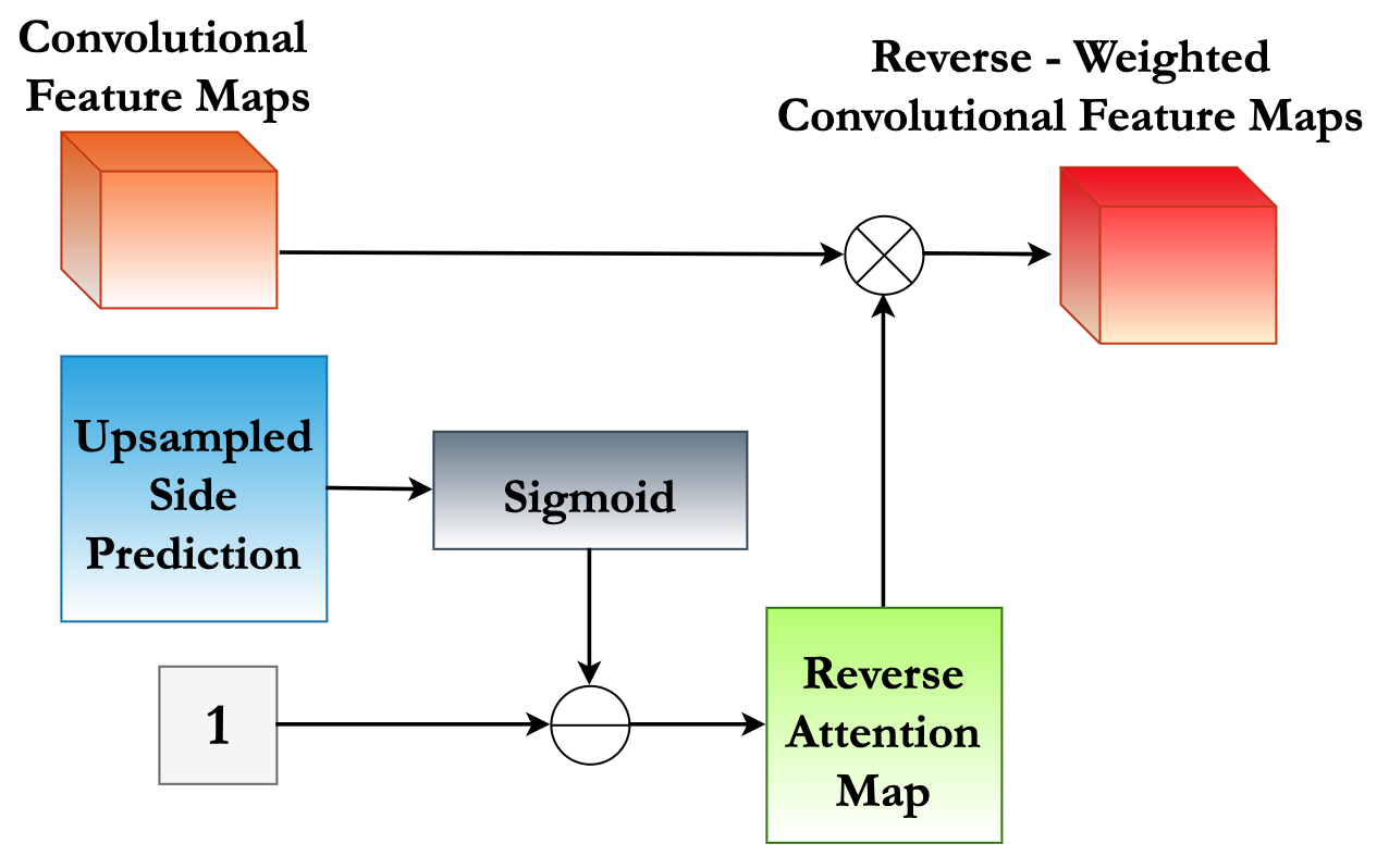
Figure 4: Reverse Attention Unit (RAU)

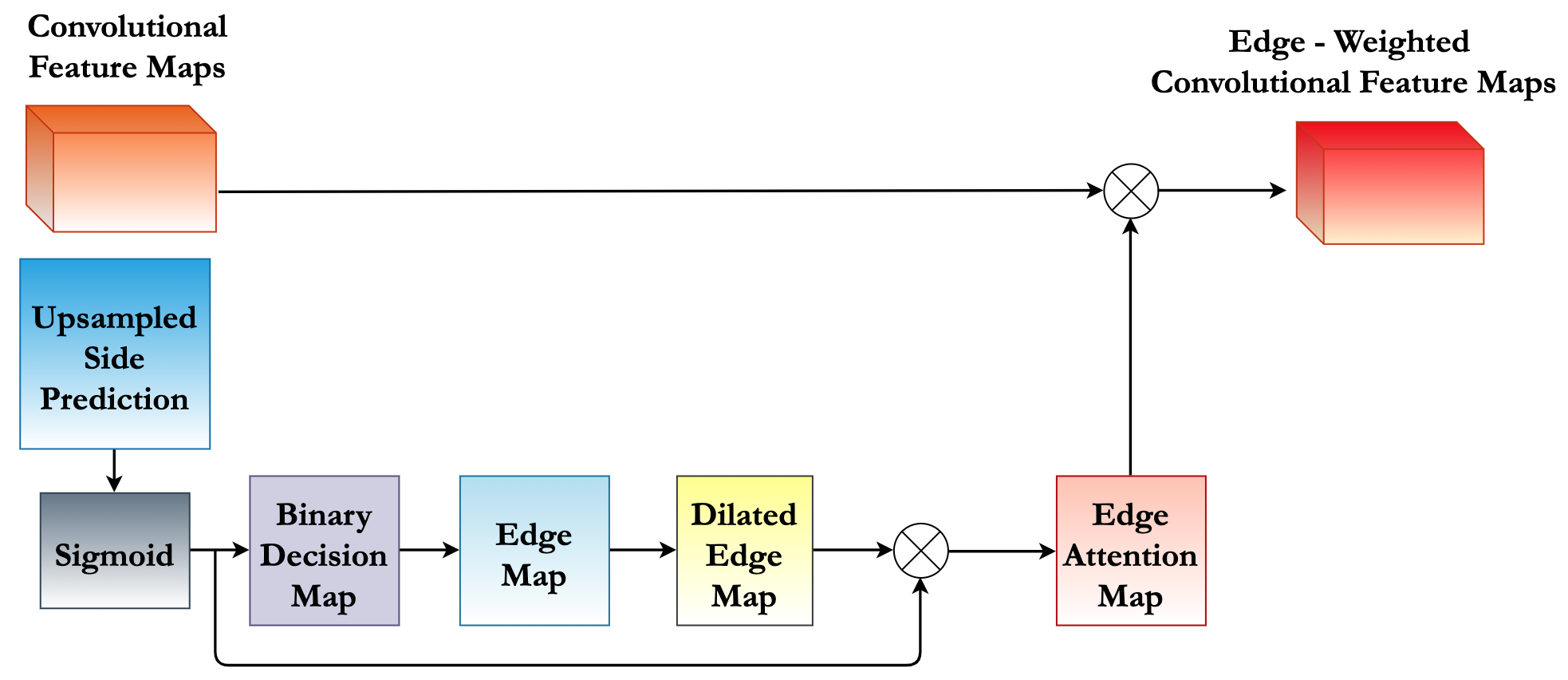
Figure 5: Edge Attention Unit (EAU)

In general, given a deep network for image segmentation, the high-level feature maps extracted in layers closer to the final output will contain accurate localization information about the objects in the image, but will be lacking in fine detail regarding those objects. On the other hand, the layers closer to the input will be rich in fine detail but with unreliable estimates of where exactly the object is located. The purpose of the Refinement Module is to fuse the fine detail from the lower-indexed layers with the spatial features in the higher-indexed layers with the expectation that such a fusion would lead to a segmentation mask that is rich in fine details and that, at the same time, exhibits high accuracy with regard to object localization.

Such a fusion in our framework is carried out by the Refinement Module that is used in each stage of the decoder for refining the prediction map gradually by recovering the fine details lost during encoding. This module does its work through two attention units: Reverse Attention Unit (RAU) and Edge Attention Unit (EAU). Through residual learning, both these units seek to improve the quality of the predictions made in the previous decoder level on the basis of the finer image detail captured during the current decoder level. What’s important here is the fact that both these actions are meant to be carried out in those regions of an image where the accuracy of semantic segmentation is likely to be poor — e.g. in the vicinity of building boundaries, as can be seen in Figure 6.

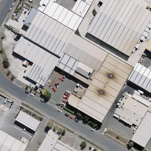
(a)

(b)

(c)

(d)

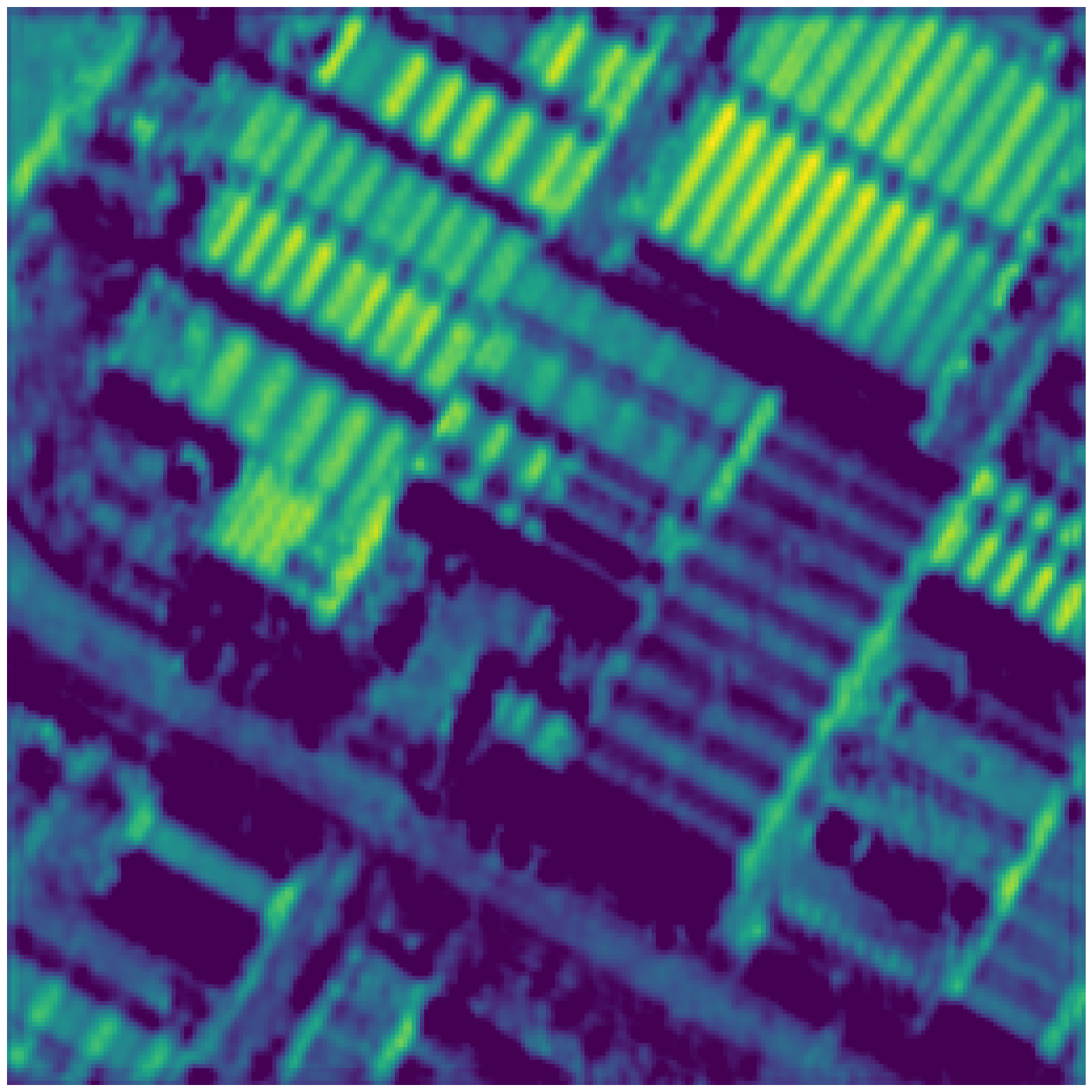
(e)

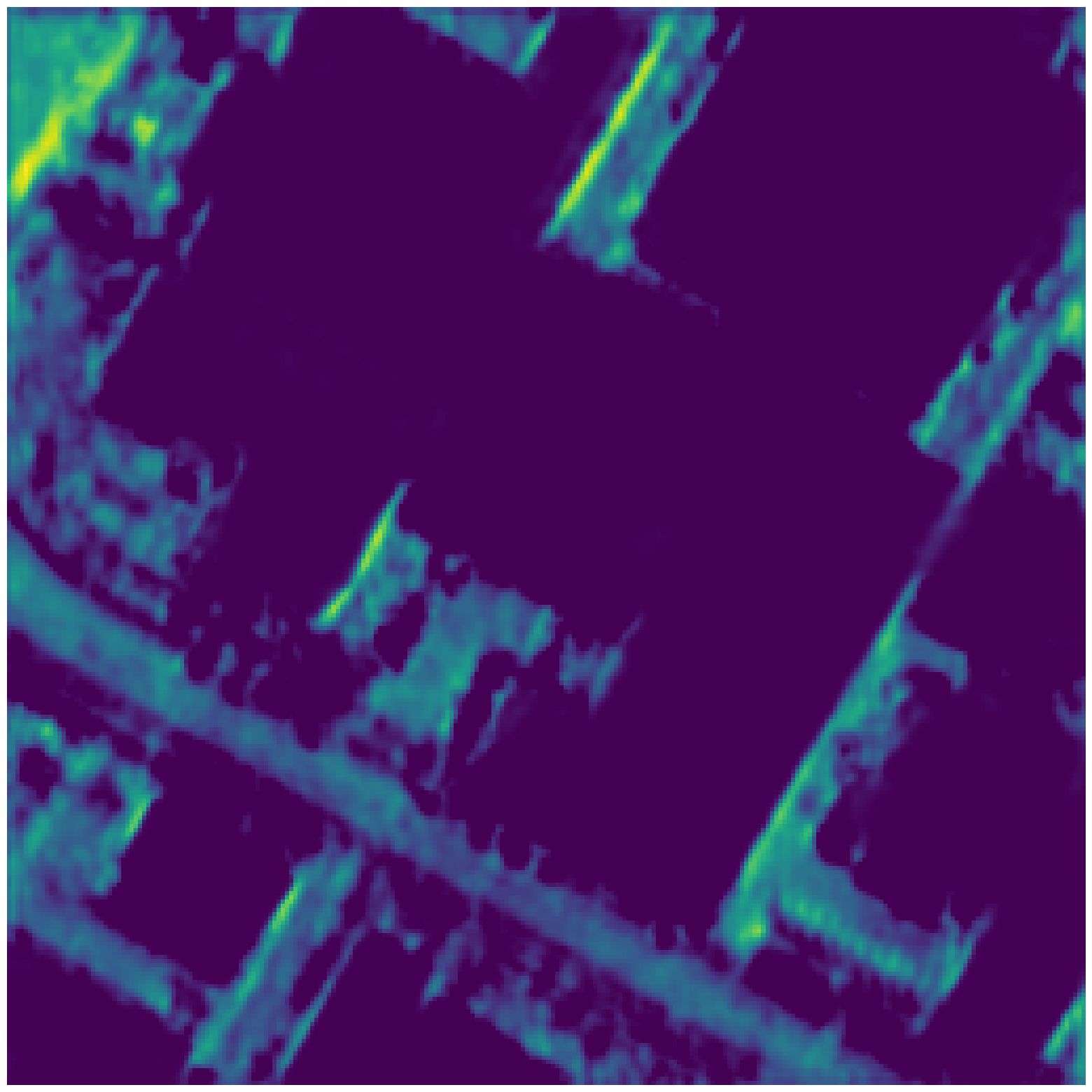
(f)

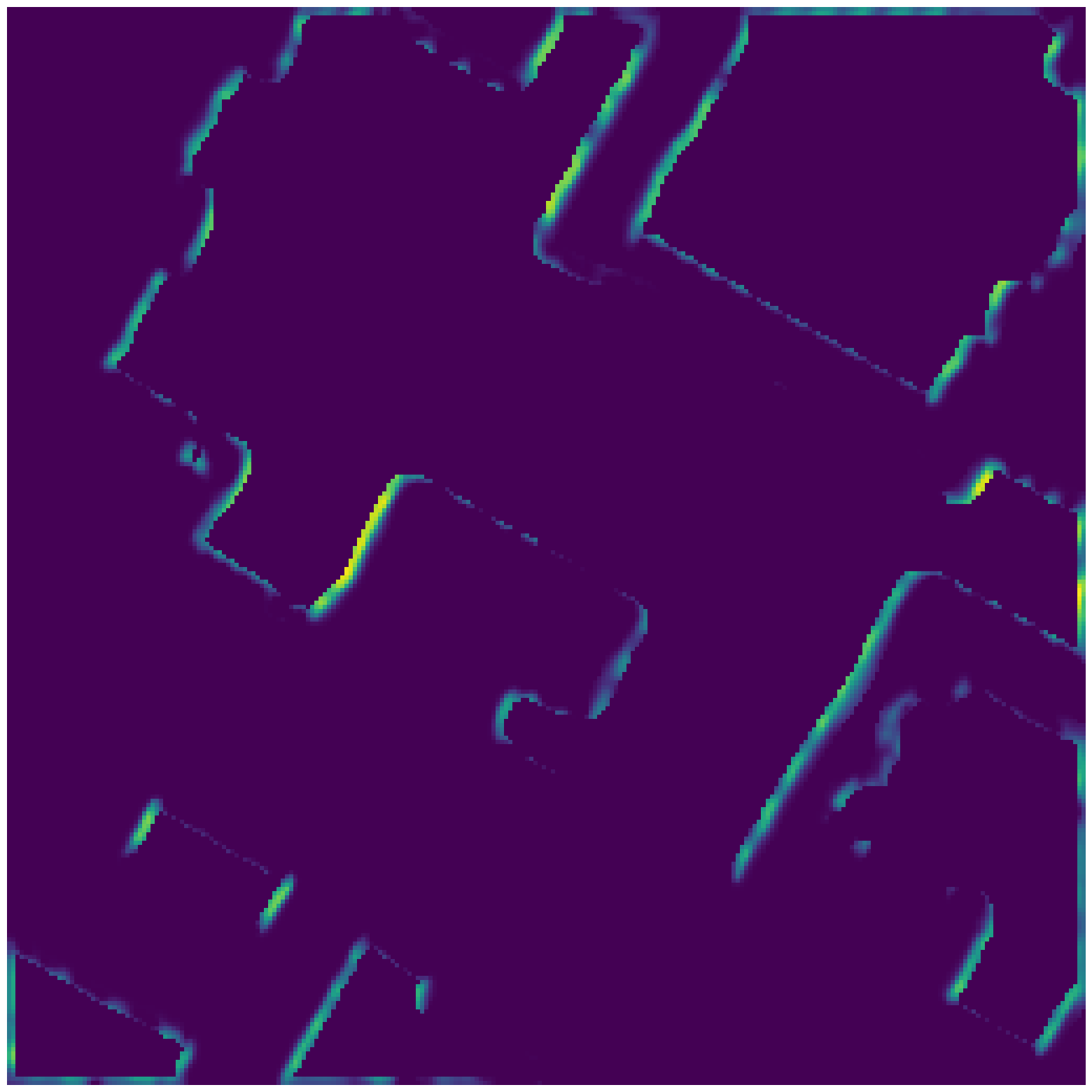
(g)

(h)

(i)

(j)

(k)

(l)

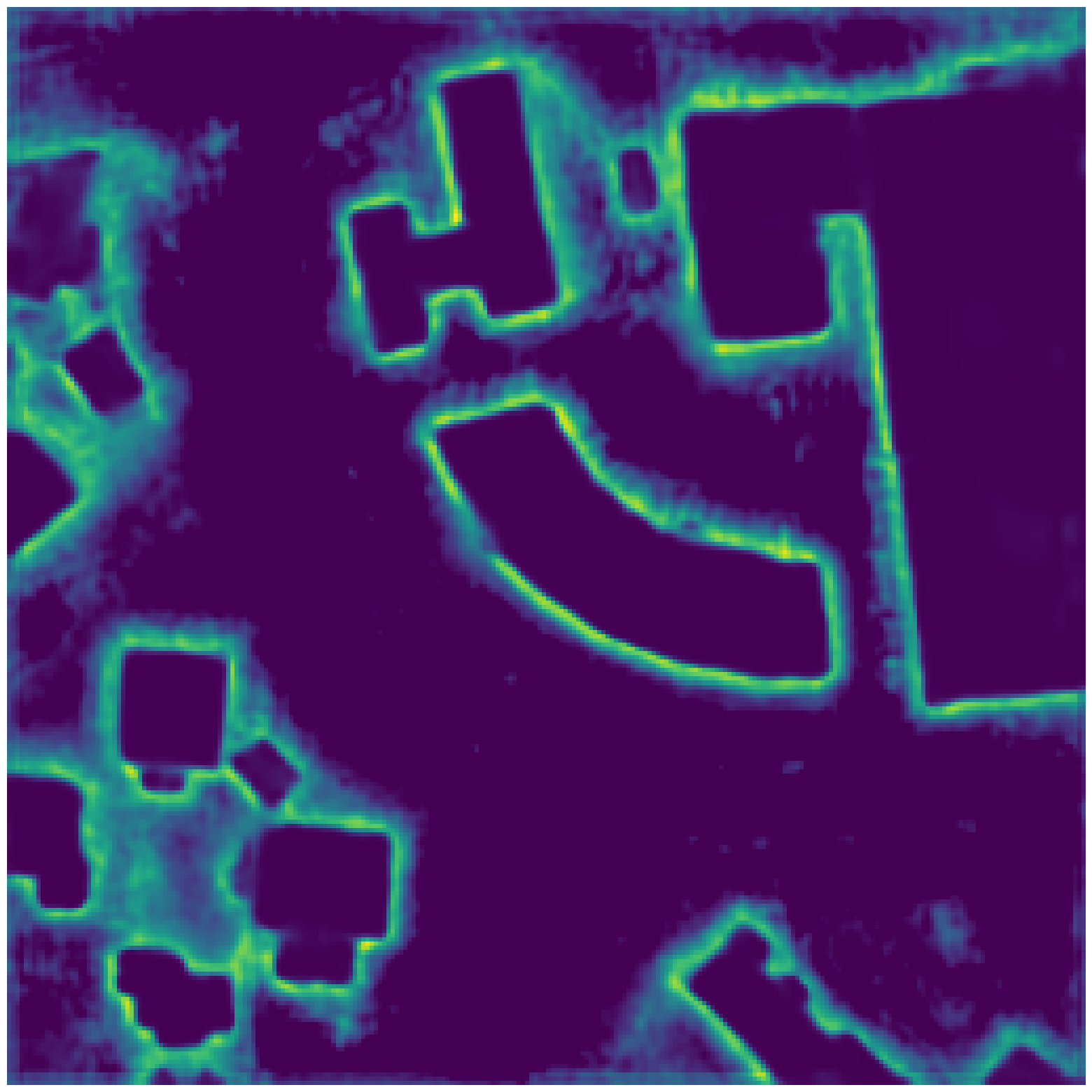
(m)

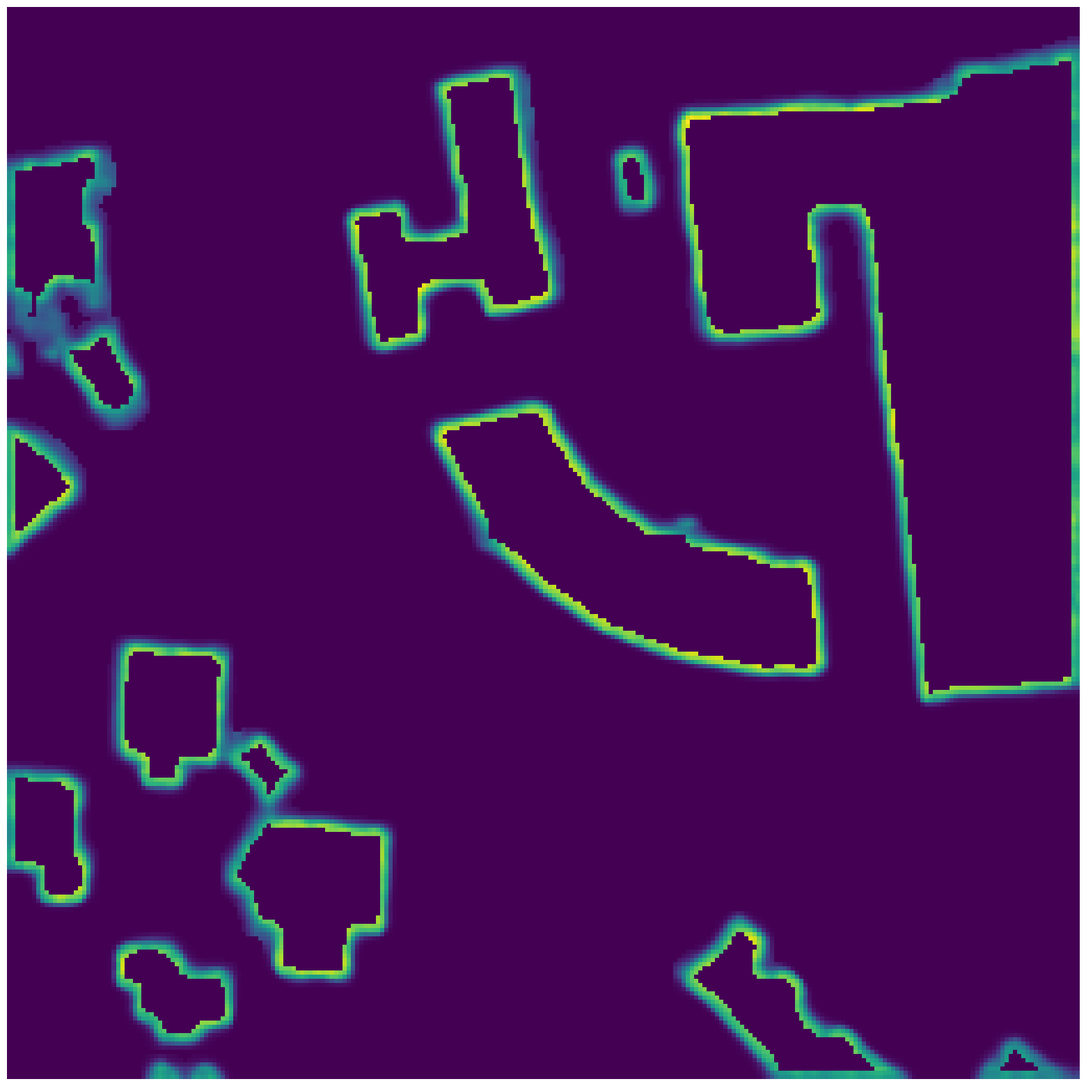
(n)

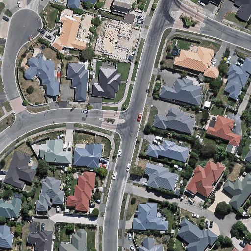
(o)

(p)

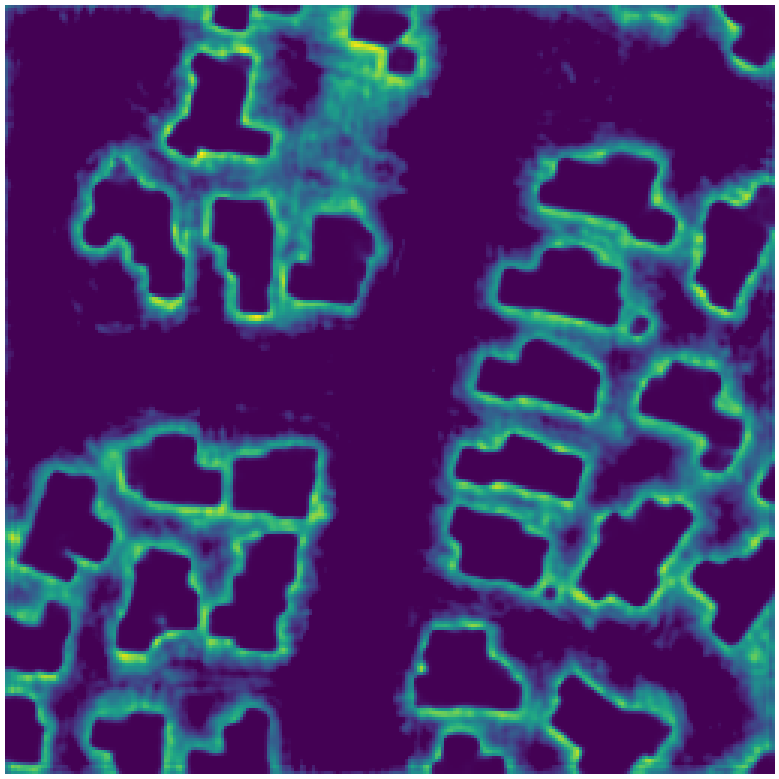
(q)

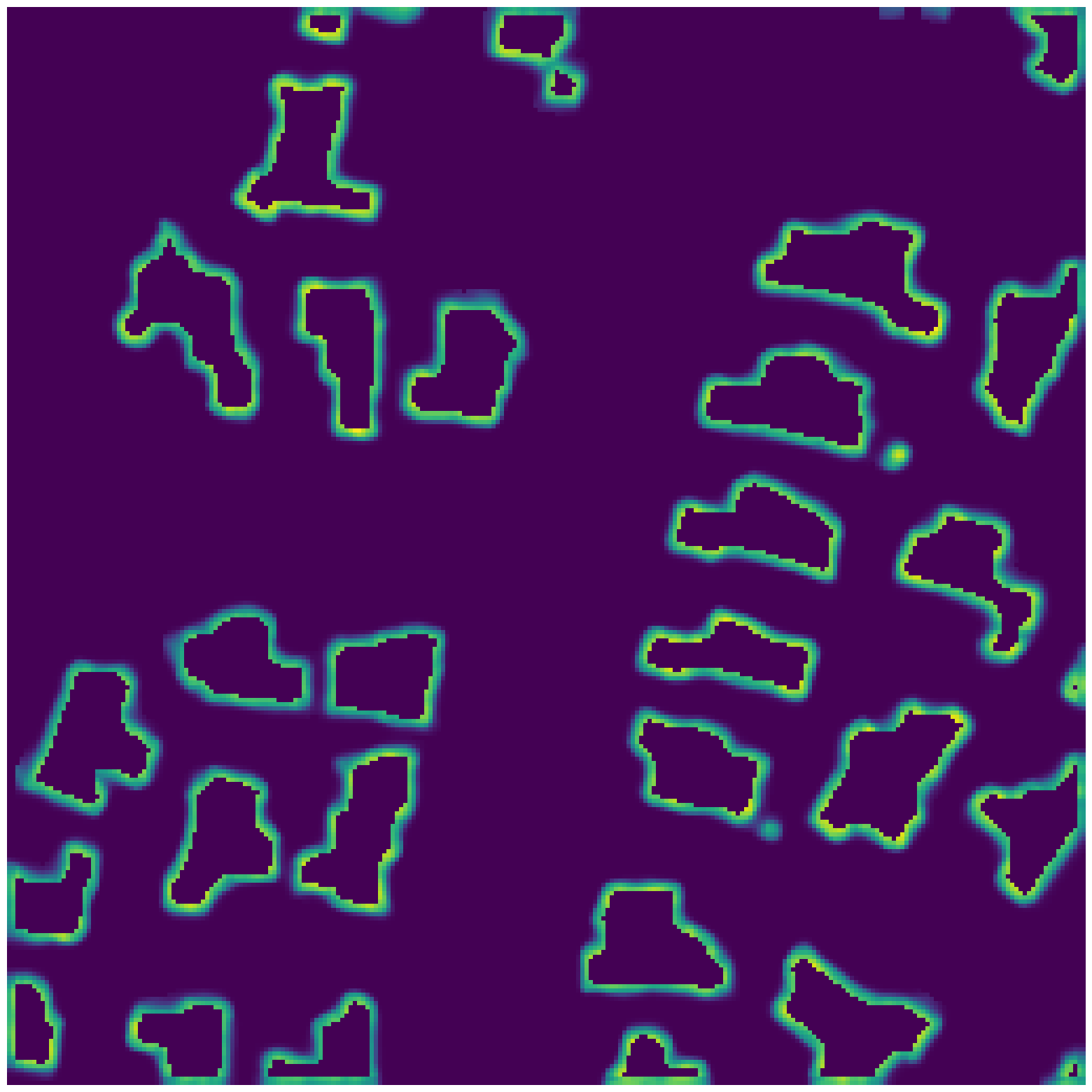
(r)

(s)

(t)

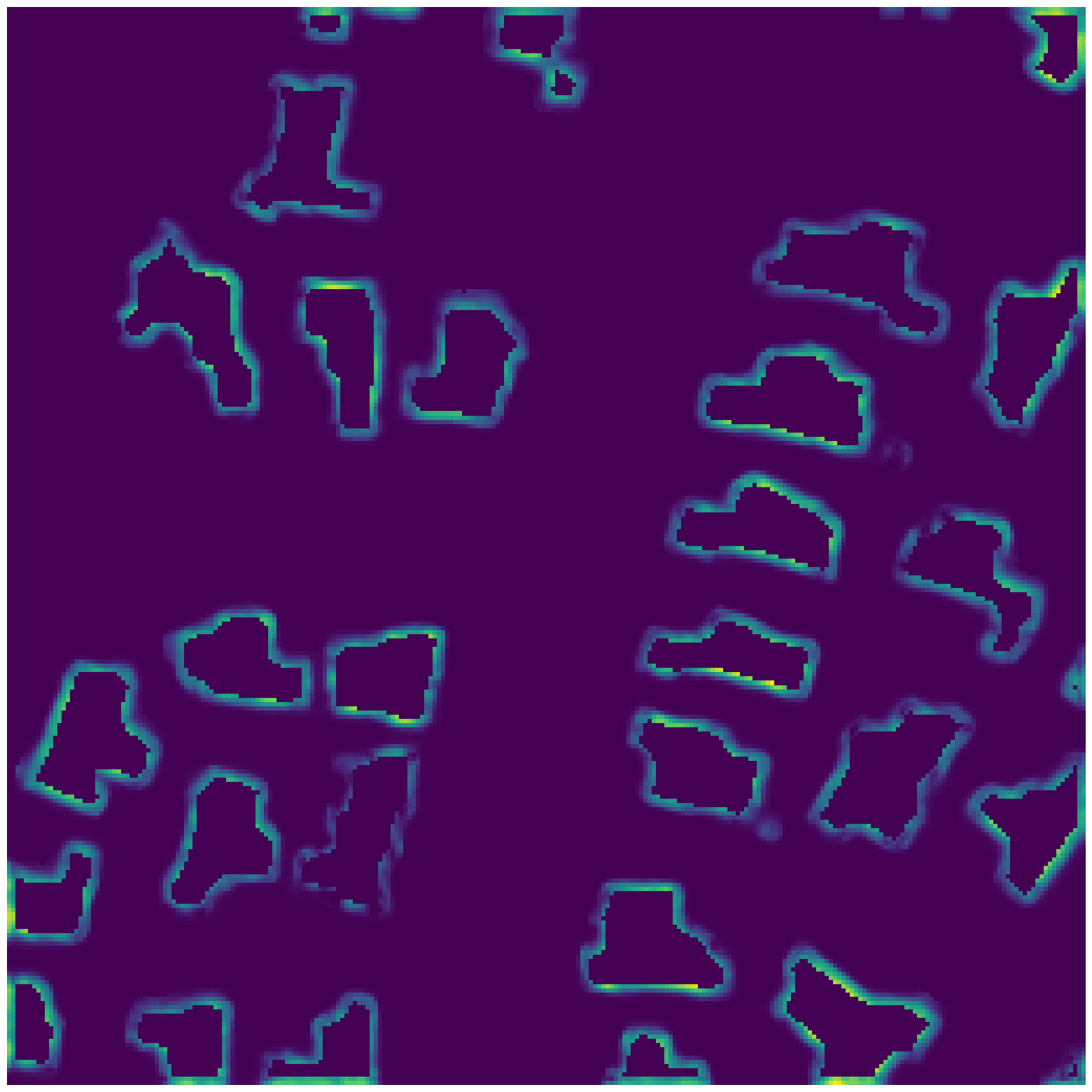
(u)

(v)

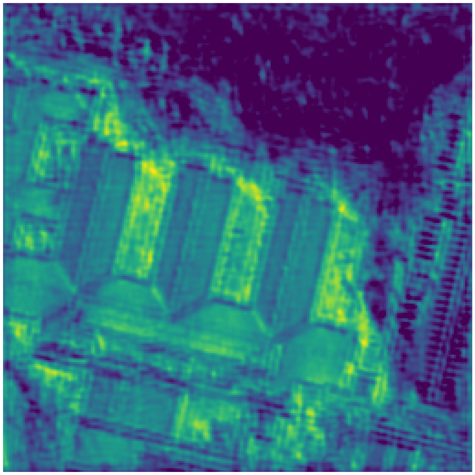
(w)

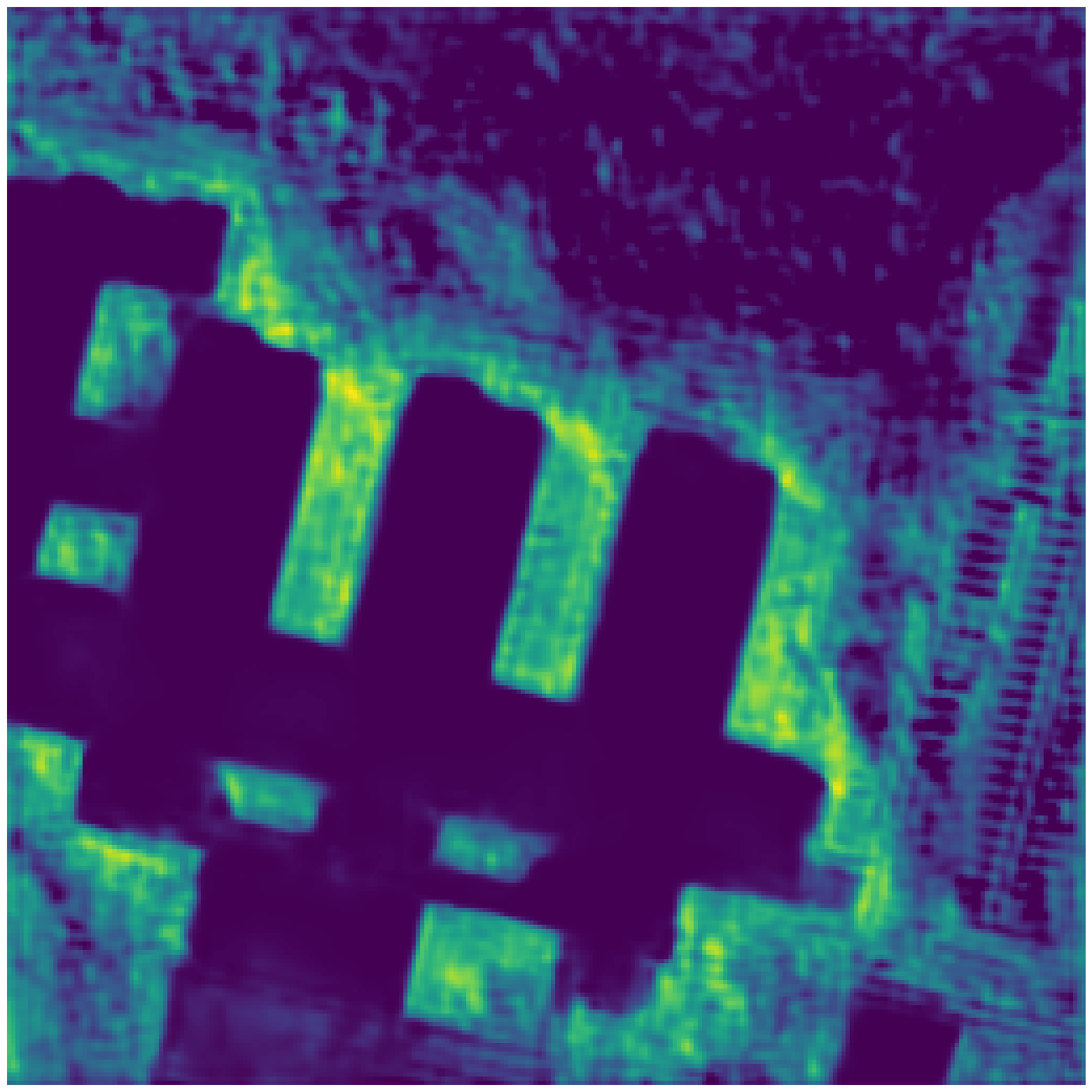
(x)

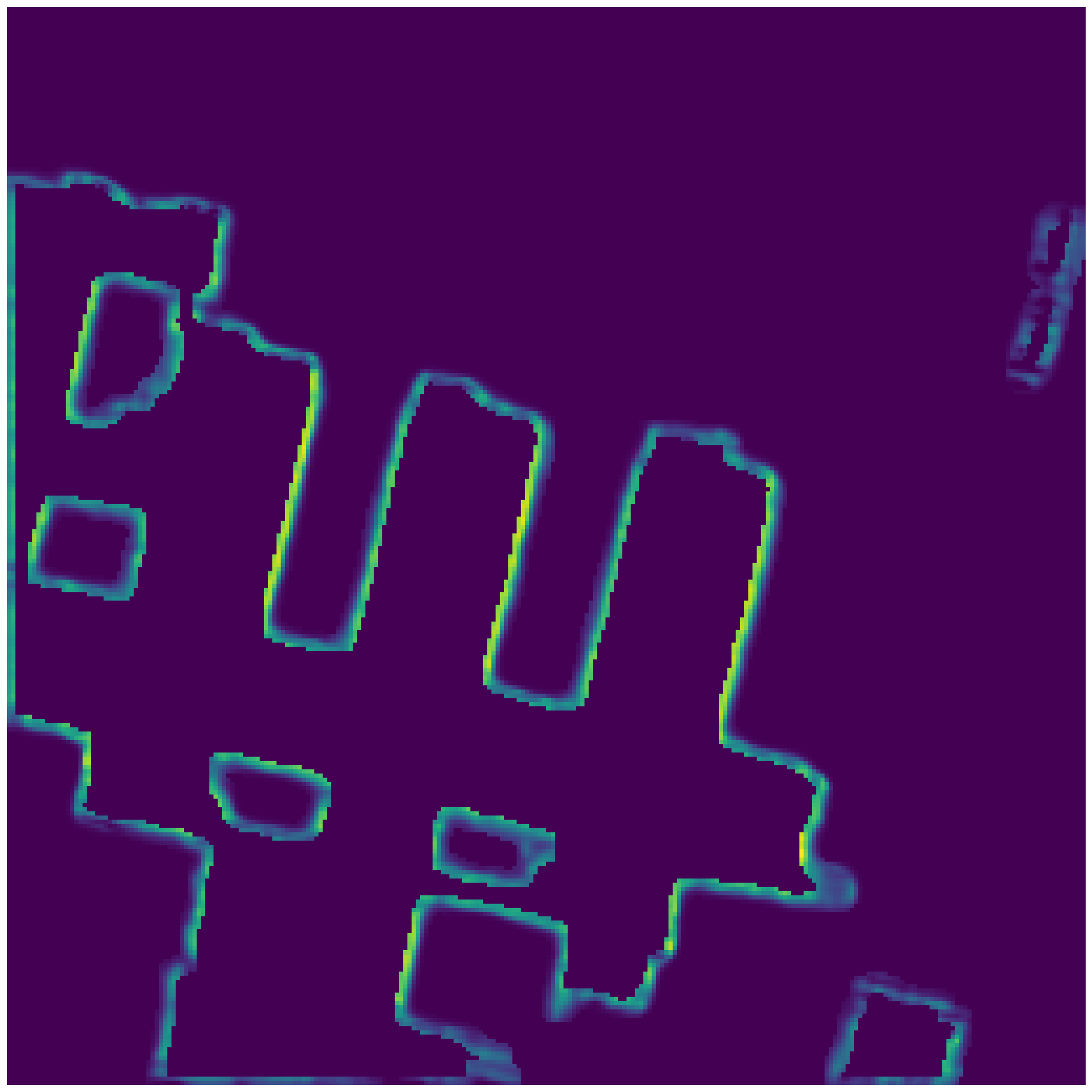
(y)

(z)

(aa)

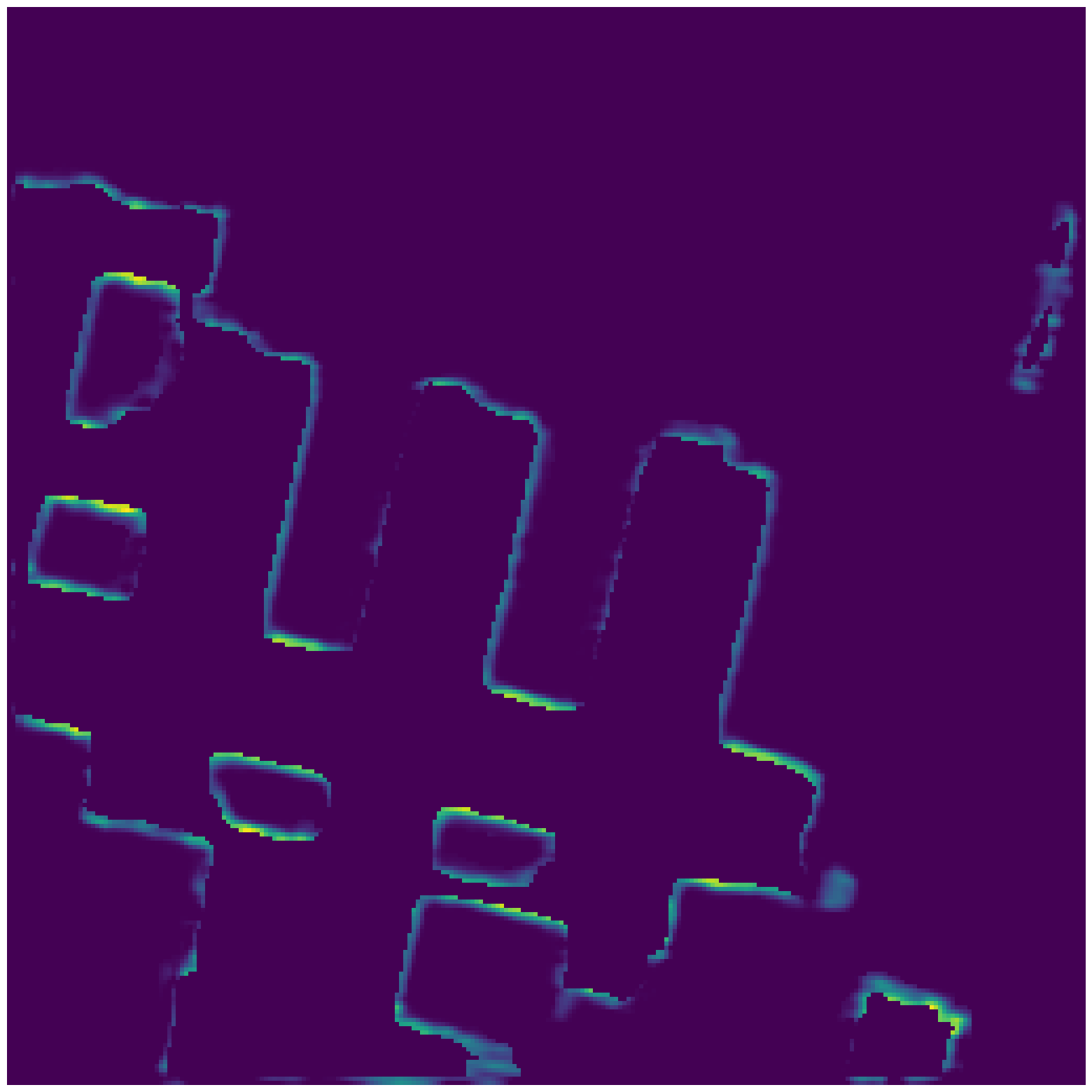
(ab)

Figure 6: Visualization of the decoder feature maps before and after applying reverse and edge attention. Column 1: Input image. Column 2, 5: Decoded Convolutional Features without any attention. Column 3, 6: Decoded Convolutional Features with Reverse Attention. Column 4, 7: Decoded Convolutional Features with Edge Attention.

For example, starting with the bottleneck, the encoded features extracted from the ASPP module predict the top-most prediction map that is at low resolution but rich in semantic information. The decoder starts with this coarse prediction map and looks back at it in the next layer of the decoder where additional image detail is available for improving the prediction probabilities that were put out by ASPP and for improving the edge detail associated with the predictions. The former is accomplished by RAU and the latter by EAU. While similar techniques have been used in the past to improve the output of semantic segmentation [73, 74] and object detection [75], we believe that ours is the first contribution that incorporates these ideas for a reliable extraction of building footprints in aerial and satellite imagery.

As shown in Figure 5, the Refinement Module concatenates the feature maps that are produced by RAU and EAU. The concatenated feature maps are then passed through two $3\times 3$ Conv layers, and the output of the Refinement Module is then added to the upsampled upper-layer prediction to obtain a finer lower-level prediction, as shown in the figure. The circle with a plus sign inside it in the figure means an element-wise addition of the two inputs. Details regarding the two attention units are presented in the next two subsections.

III-B1a Reverse Attention

The idea of reverse attention is to reconsider the predictions coming out of a lower-indexed layer in the decoder in light of the spatial details available at the current layer. This amounts to a backward look in the decoder chain and justifies the name of this attention unit.

Figure 5 illustrates how the reverse attention mechanism works. The RAU takes two inputs: (1) the upsampled version of the building prediction map produced by the previous decoder layer; and (2) the finer detailed Conv features copied over from the encoder side after they have been processed by the decoder logic in the current layer. As should be evident from the data flow arrows in Figure 2, the Reverse Attention Unit (RAU) guides the network to use the fine detail in the current layer of the decoder and reevaluate the building predictions coming out of the lower layer. We refer to these reassessed predictions as Reverse Attention Map. At the $n^{th}$ layer, the Reverse Attention Map is generated as follows:

$$A_{R}^{n}=1-Sigmoid(U(P_{n-1}))$$ (1)

where $P_{n-1}$ is the building prediction map produced by the $(n-1)^{th}$ layer and $U(P_{n-1})$ is its upsampled version that can be understood directly in the $n^{th}$ layer.

There is a very important reason for the subtraction in the equation shown above: As one would expect, the building detection probabilities are poor near the building edges and that’s exactly where we want to direct RAU’s firepower, hence the reversal of the probabilities in the equation shown above. As it turns out, this is another reason for “Reversal” in the name of this attention unit.

We now define a Reverse–Weighted Feature Map, $F^{n}_{R}$, for the $n^{th}$ layer:

$$F_{R}^{n}=A_{R}^{n}\otimes F_{n}$$ (2)

where the symbol $\otimes$ denotes element-wise multiplication, and $F_{n}$ represents the convolutional feature maps of the $n^{th}$ layer.

III-B1b Edge Attention

The purpose of the edge attention is to improve the quality of the boundary edges of the building predictions made by the previous layer of the decoder using the additional image detail available in the current layer.

Essential to the logic of what improves the boundary edges is the notion of contour extraction. At each layer on the decoder side, we want to extract the contours in the fine detail provided by the encoder side in order to improve the edges in the building prediction map yielded by the lower layer. Note that there is a significant difference between just detecting the edge pixels and identifying the contours. Whereas the former could yield just a disconnected set of pixels on the object edges, the latter is more likely to yield a set of connected boundary points — even when using just contour fragment (as opposed to, say, closed contours). On account of the need to make these calculations GPU compatible, at the moment the notion of contour extraction is carried out by applying the Sobel edge detector [76] to a building prediction map followed by a p-pixel dilation of the edge pixels identified in order to connect what would otherwise be disconnected pixels.

As shown in Figure 5, the Edge Attention Unit (EAU) takes two inputs: 1) the upsampled version of the building prediction map produced by the previous decoder layer; and 2) the finer detailed convolutional features copied over from the encoder side after they have been processed by the decoder logic in the current layer. The output of EAU consists of an edge-weighted feature map. If $n$ denotes the index for the current layer in the decoder, the building prediction map produced by the previous layer, denoted $P_{n-1}$, is first upsampled using bilinear interpolation to get $U(P_{n-1})$, which is then used to generate a binary decision map, $B_{E}^{n}$, for the current layer as follows:

$$B_{E}^{n}=\begin{cases}1&\text{if $Sigmoid(U(P_{n-1}))\geq$ 0.5}\\ 0&\text{otherwise}\\ \end{cases}$$ (3)

Subsequently, the Sobel edge detector is applied to the binary decision map in order to detect edge fragments in the predicted binary map. As shown in Figure 5, the next step is to dilate the edge fragments produced by Sobel so that they become $p$-pixels wide. The edge dilation step connects what could otherwise be disjoint edge fragments. Typically, we dilate the edge pixels by a kernel of size $7\times 7$ to get a dilated edge map, $D_{E}^{n}$, which leads to the edge attention map as defined by:

$$A_{E}^{n}=Sigmoid(U(P_{n-1}))\otimes D_{E}^{n}$$ (4)

The edge attention map could be thought of as a boundary confidence map. This confidence map is then multiplied with the $n^{th}$ layer feature map to obtain the edge-weighted features, $F_{E}^{n}$ as shown below:

$$F_{E}^{n}=A_{E}^{n}\otimes F_{n}$$ (5)

where $F_{n}$ is the $n^{th}$ layer feature map.

III-B2 Uncertainty Attention

In general, a classical encoder-decoder network does not provide for feature selection when fusing together the high-level features going through decoder with the low-level features being copied over from the encoder side through the skip connections. A manifestation of this phenomenon is over-segmentation in the final output of the network that is caused by indiscriminately fusing the low-level features from the encoder with the high-level features in the decoder.

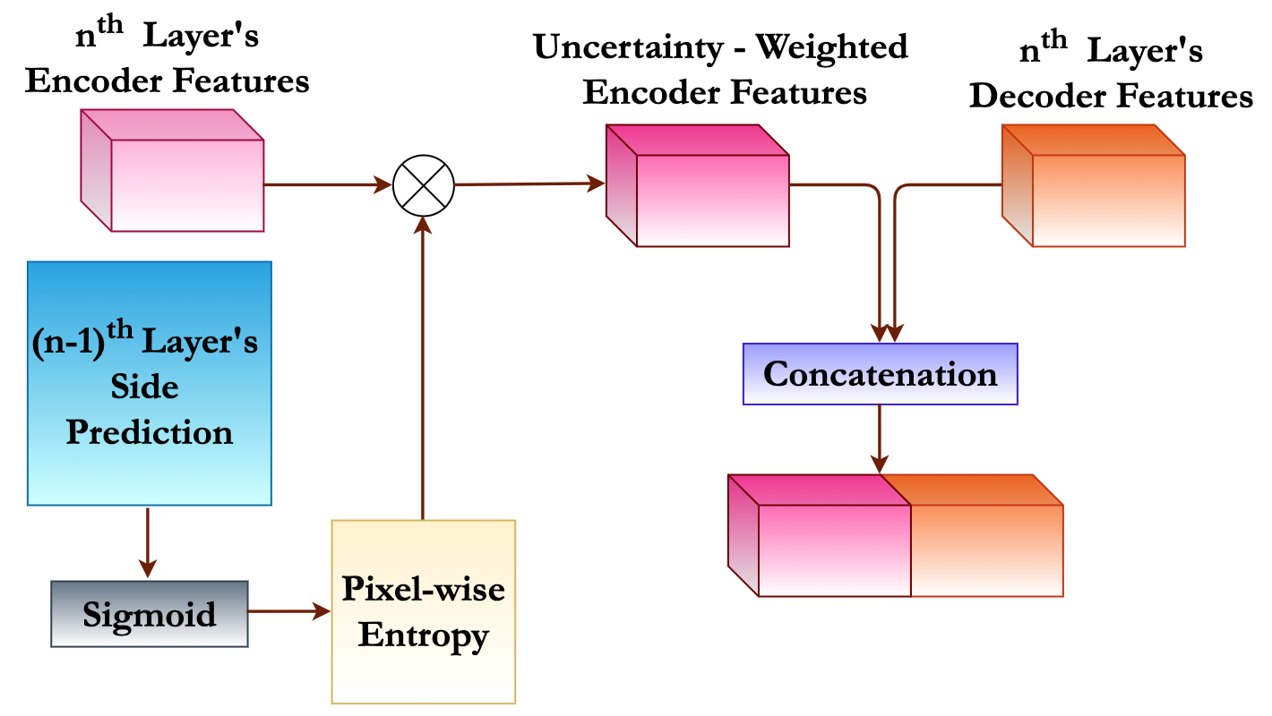
Figure 7: Uncertainty Attention Module (UAM)

To mitigate such over-segmentations, we introduce an Uncertainty Attention Module in every encoder-to-decoder skip connection, as shown by the yellow boxes in the middle of the ‘U’ in Figure 2. The purpose of these attention units is to mediate the level of inclusion for the encoder-generated low-level features when they are copied over to the decoder side. More specifically, we want the Uncertainty Attention Module to use the low-level detail made available by the encoder only in those regions of a prediction map where the degree of uncertainty exceeds a threshold. Experience with such architectures tells us that we can expect the uncertainty to be relatively large in the vicinity of the object boundaries in the input images, as can be seen in Figure 8.

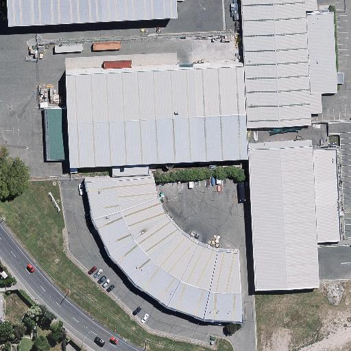
(a)

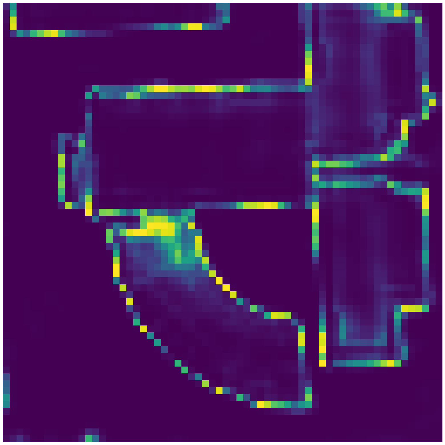
(b)

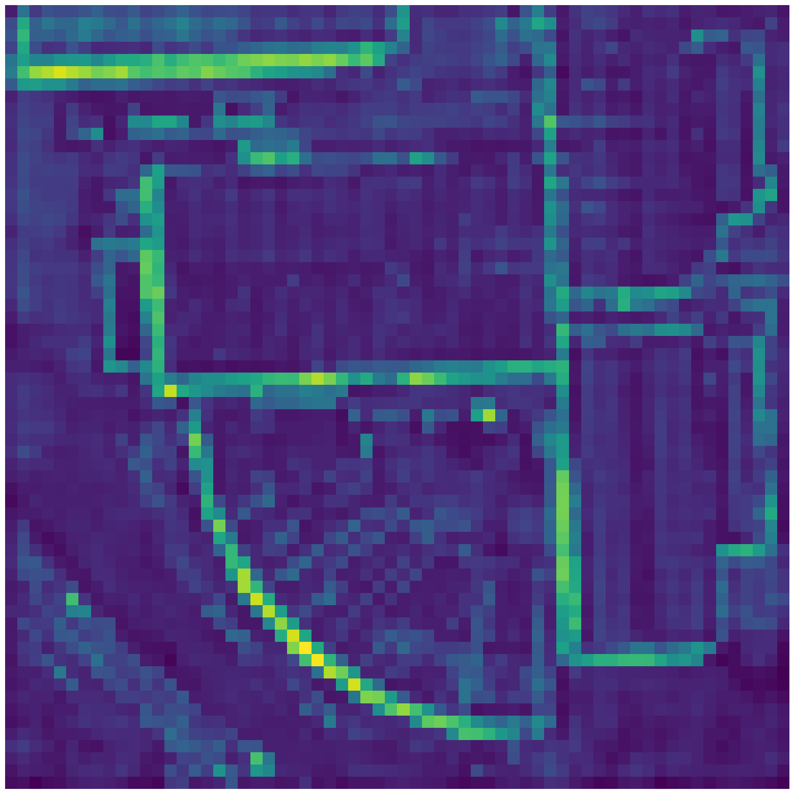
(c)

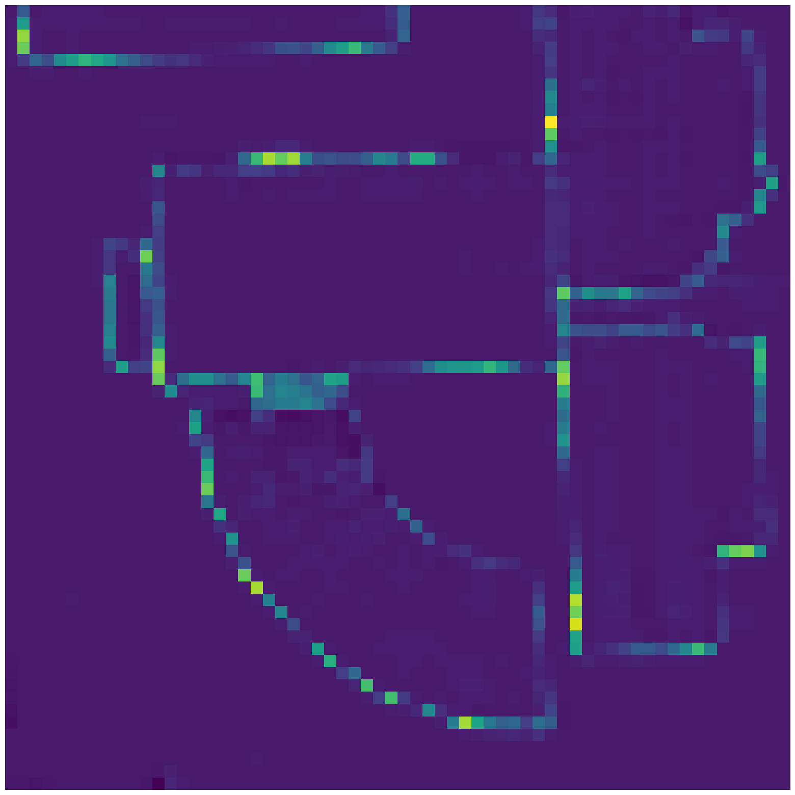
(d)

(e)

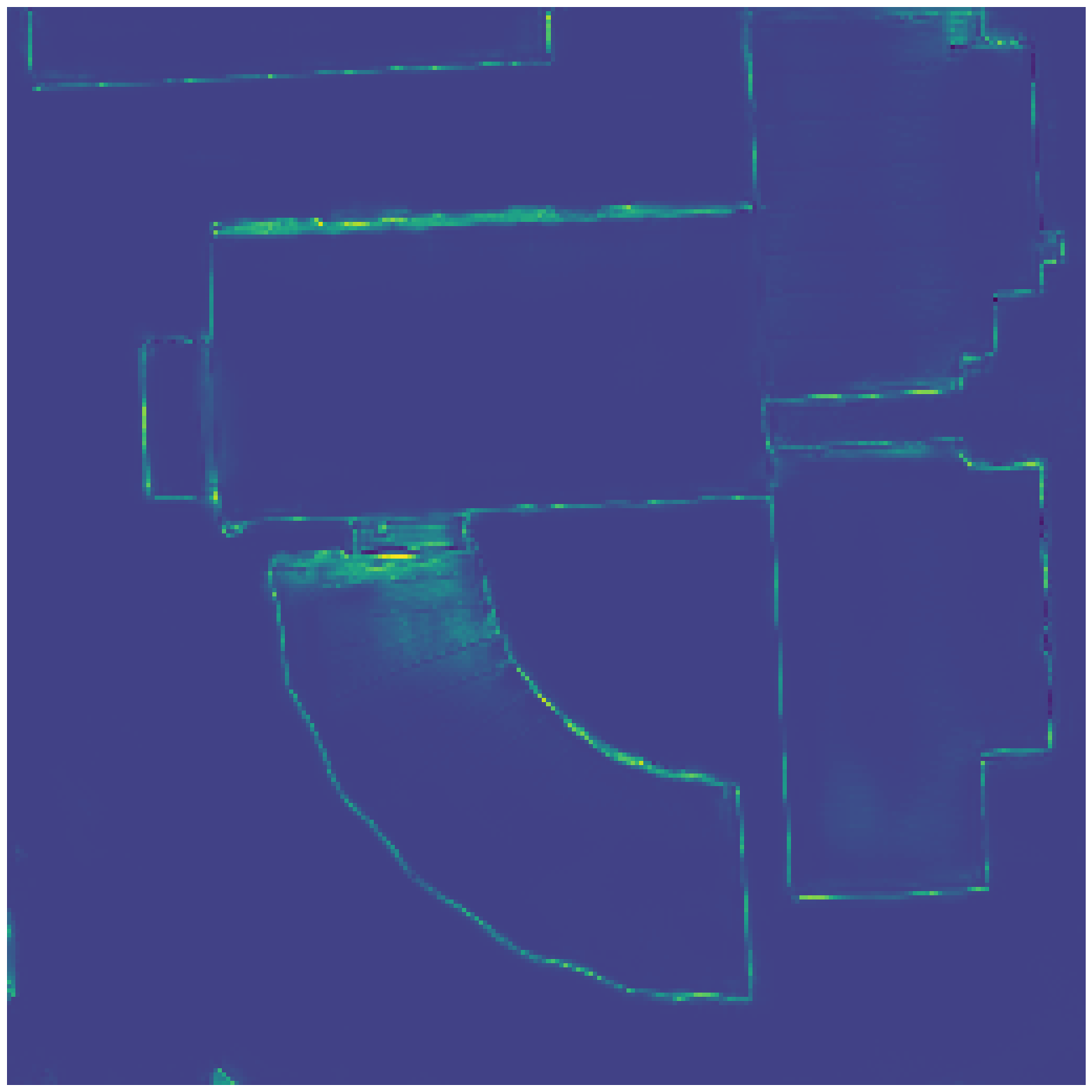
(f)

(g)

(h)

(i)

(j)

(k)

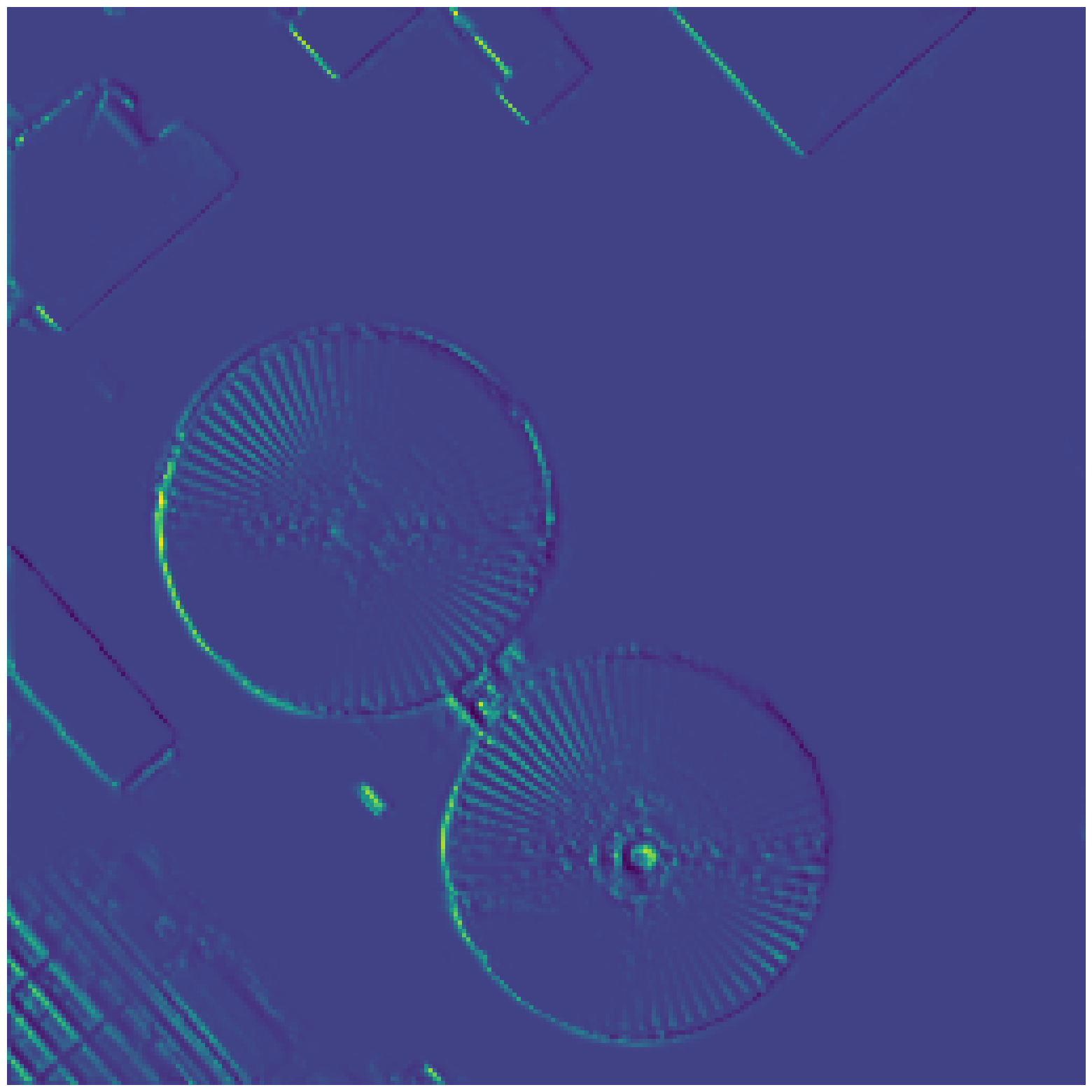
(l)

(m)

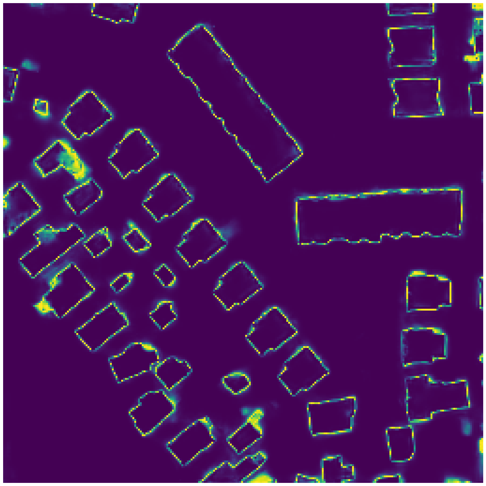
(n)

(o)

(p)

(q)

(r)

(s)

(t)

(u)

(v)

(w)

(x)

Figure 8: Visualization of the encoder feature maps before and after applying uncertainty attention. Column 1: Input image. Column 2: Uncertainty Attention Map. Columns 3, 5: Encoder Features without Uncertainty Attention. Column 4, 6: Corresponding Encoder Features with Uncertainty Attention.

That raises the question of how to measure the degree of uncertainty associated with the predictions on the decoder side. As it turns out, that’s an easy thing to do by measuring the entropy associated with the building predictions in the different levels of decoder. We compute pixel-wise entropy in a prediction map to produce the uncertainty attention map at each level of our network as follows:

$$E(i)=-p_{i}\>\log(p_{i})-(1-p_{i})\>\log(1-p_{i})$$ (6)

where $p_{i}$ denotes the probability of the $i^{th}$ pixel belonging to the building class. This uncertainty attention map is then element-wise multiplied with the low-level feature maps in that specific layer to create an uncertainty–weighted low-level feature map, as shown in Figure 7.

Recent research [77] has shown that concatenating shallow encoder features with deep decoder features can adversely affect the predictions if the semantic gap between the features is large. And, it stands to reason that introducing uncertainty attention prior to concatenation has the possibility of amplifying this problem by injecting “noisy” encoder features in those regions of a building prediction map where the probabilities are low. We guard against such corruption of the prediction maps by using deep supervision (shown by thick arrows in Figure 2) that forces the intermediate feature maps to be discriminative at all levels of the docoder. Deep supervision [78, 79, 80, 81] allows for more direct backpropagation of loss to the hidden layers of the network.

III-C Critic Network

We now present the details regarding the critic network ($\mathcal{C}$) in our framework. The network for $\mathcal{C}$ is essentially the same as the encoder in $\mathcal{S}$ minus the residual blocks. Our experiments have shown that adding the residual blocks in $\mathcal{C}$ increase the parameter space of the model without any significant improvement in the performance of the critic.

$\mathcal{C}$ is supplied with two inputs: (a) 3-channel remotely sensed images masked by the corresponding ground-truth building labels; and (b) 3-channel remotely sensed images masked by the building labels generated by $\mathcal{S}$. These masks (predicted and the ground-truth) are created by element-wise multiplication of the one-channel label maps with the original RGB images, as shown in Figure 9. $\mathcal{C}$ extracts features from the predicted mask as well as the ground-truth mask at multiple scales, reshapes these multi-scale features into one-dimensional vectors and concatenate them together. Finally, $\mathcal{C}$ seeks to maximize the difference between the vectors created from the true instances and the predicted instances.

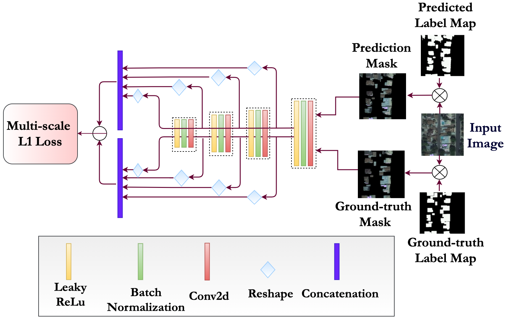
Figure 9: Critic Framework

.

IV Training Strategy

The generator i.e. the segmentor ($\mathcal{S}$) and the critic ($\mathcal{C}$) in our proposed architecture are trained alternatively in an adversarial fashion. $\mathcal{S}$ tries to predict an accurate label map for the buildings present in the input image such that $\mathcal{C}$ cannot distinguish between the predicted map and the ground-truth map, whereas $\mathcal{C}$ aims to discriminate the predicted maps from the ground-truth maps. To train the network in an adversarial fashion, we calculate the multi-scale ${L}_{1}$ loss, as explained in Section IV-A, using the hierarchical features extracted from the multiple layers of $\mathcal{C}$. This multi-scale ${L}_{1}$ loss, proposed by Xue et al. in [14], enables the network to capture the long and short range spatial relations between the pixels. First, we train $\mathcal{C}$ keeping the parameters of $\mathcal{S}$ fixed and try to minimize the negative of ${L}_{1}$ loss. Next, we keep the parameters of $\mathcal{C}$ fixed and train $\mathcal{S}$ minimizing the same ${L}_{1}$ loss. Moreover, we incorporate extra supervision in the form of weighted dice and shape losses to stabilize the training of $\mathcal{S}$ and boost its performance.

IV-A Adversarial Loss: Multi-scale ${L}_{1}$ Loss

We define our adversarial loss function ${L}_{1}$ as:

$${L}_{1}=\frac{1}{N}\sum_{i=1}^{N}l_{mae}(f_{C}(x_{i}\circ S(x_{i})),f_{C}(x_{i}\circ y_{i}))$$ (7)

where $N$ is the batch size and $x_{i}$ is the $i^{th}$ image in a batch. The notation $S(x_{i})$ stands for the output label map of $\mathcal{S}$, and $y_{i}$ is the corresponding ground-truth label map. The notation $x_{i}\circ S(x_{i})$ stands for the original input sample masked by predicted map and $x_{i}\circ y_{i}$ is the input image masked by the ground-truth label map. The notation $f_{C}(x)$ stands for the features extracted from the image $x$ in multiple layers of $\mathcal{C}$ and $l_{mae}$ stands for the Mean Absolute Error (MAE) defined as:

$$l_{mae}(f_{C}(x),f_{C}(y))=\frac{1}{L}\sum_{k=1}^{L}\|(f^{k}_{C}(x)-f^{k}_{C}(y))\|_{1}$$ (8)

where $f^{k}_{C}(x)$ is the feature map extracted from the image $x$ at the $k^{th}$ layer of $\mathcal{C}$, the subscript $mae$ stands for “mean absolute error”, ‘$L$’ is the number of layers in $\mathcal{C}$, and $\|.\|_{1}$ represents $\ell 1$ norm.

IV-B Joint Dice and Shape Loss

The overall loss function used also includes dice and shape losses for stabilizing the training of $\mathcal{S}$ and for boosting its performance. We have observed that only using adversarial loss leads to unstable training of the GAN. The dice part of the loss, shown below in Eq. (9), optimizes the dice similarity coefficient (DSC) and the shape part of the same, shown in Eq. (10), minimizes the Hausdorff Distance (HD) [82] between the ground-truth and prediction.

Here is the formula used for the dice loss:

$$L_{dice}= 1-\left[\alpha_{1}\frac{2*\sum_{i}^{N}p_{i}g_{i}}{\sum_{i}^{N}p_{i}^{2}+\sum_{i}^{N}g_{i}^{2}}\right.$$ (9)

$$\left.+\alpha_{2}\frac{2*\sum_{i}^{N}(1-p_{i})(1-g_{i})}{\sum_{i}^{N}(1-p_{i})^{2}+\sum_{i}^{N}(1-g_{i})^{2}}\right]$$

where $\alpha_{1}+\alpha_{2}=1$. $\alpha_{1}$, $\alpha_{2}\geq 0$. $p_{i},g_{i}$ represent, respectively, the $i^{th}$ pixel of the ground-truth and the prediction map. This way, in addition to the contribution from the positive samples, we also ensure contribution from the negative samples. This becomes particularly useful if an entire sample is composed of only foreground or only background class. In our experiments, we set $\alpha_{1}=0.8$.

Regarding the shape loss, it helps the system keep a check on the shape similarity between the ground-truth and predicted building labels by minimizing the HD distance between them. Hausdorff Distance loss aims to estimate HD from the CNN output probability so as to learn to reduce HD directly. Specifically, HD can be estimated by the distance transform of ground-truth and segmentation. We compute the average shape loss as follows -

$$L_{HD}=\frac{1}{N}\sum_{i=1}^{N}\left[(p_{i}-g_{i})^{2}(d_{p_{i}}^{2}+d_{g_{i}}^{2})\right]$$ (10)

where $d_{p_{i}}$ and $d_{g_{i}}$ are the taxicab (i.e. $\ell 1$) distance transforms of the ground-truth and predicted label maps.

V Datasets and Evaluation Metrics

In this paper, we show results on four publicly available datasets - Massachusetts Buildings (MB) Dataset [1], INRIA Aerial Image Labeling Dataset [15], WHU Building Dataset [54] and DeepGlobe Building Detection Dataset [71, 72]. These datasets cover different regions of interest across the world and include diverse building characteristics. We have used different evaluation metrics for different datasets in order to carry out a fair comparison with the other state-of-the-art methods.

V-A Massachusetts Buildings Dataset

The Massachusetts Buildings (MB) Dataset [1] consists of 151 high-resolution aerial images of urban and suburban areas around Boston. Each image is $1500\times 1500$ pixels and covers an area of $2250\times 2250m^{2}$. The dataset is randomly divided into training (137 tiles), validation (4 tiles), and testing (10 tiles) subsets.

We now elaborate on the metrics that we have used for comparisons. For the Massachusetts Buildings Dataset, we report relaxed as well as non-relaxed (i.e. regular) versions of F1-score and IoU score. We use the relaxed version of precision, recall, and F1-score to calculate the precision-recall breakeven point as in [1]. A relaxation factor of $\rho$ was introduced to consider a building prediction correct if it falls within a radius of $\rho$ pixels of any ground-truth building pixel. This relaxation factor is used to provide a realistic performance measure because the building masks in the Massachusetts Buildings Dataset are not perfectly aligned to the actual buildings in the images. The formula for the F1-measure is:

$$F1=2\times\frac{precision\times recall}{precision+recall}$$ (11)

where

$$precision=\frac{tp}{tp+fp}$$ (12)

$$recall=\frac{tp}{tp+fn}$$ (13)

The relaxed version of precision denotes the fraction of predicted building pixels that are within a radius of $\rho$ pixels of a ground-truth building pixel, and the relaxed version of recall represents the fraction of the ground-truth building pixels that are within a radius of $\rho$ pixels of a predicted building pixel. To conduct a fair comparision with previous research [11, 4], we set $\rho=3$.

V-B INRIA Aerial Image Labeling Dataset

This dataset [15] features aerial orthorectified color imagery having a spatial resolution of 0.3m with a coverage of $810km^{2}$ and contains publicly available ground-truth labels for the building footprints in the training and validation subsets. The images range from densly populated areas like San Francisco to sparsely populated areas in the alpine regions of Austria. Thus, the dataset represents highly contrasting terrains and landforms. Moreover, the population centers in the training subset are different from those in the testing subset, which makes the dataset very appropriate for assessing a network’s generalization capability.

The training set contains 180 color image tiles of size $5000\times 5000$, covering a surface of $1500\times 1500m^{2}$ each (at a 0.30m resolution). There are 36 tiles for each of the following regions: Austin, Chicago, Kitsap County, Western Tyrol and Vienna. Each tile has a correspinding one-channel label image indicating buildings (255) and the not-building class. The test set also contains 180 tiles but from different areas: Bellingham (WA), Bloomington (IN), Innsbruck, San Francisco and Eastern Tyrol.

The performance measures used for this dataset are: (a) Intersection over Union (IoU): number of pixels labeled as building in both the prediction and the ground truth, divided by the number of pixels labeled as pixel in the prediction or the ground-truth, and, (b) Accuracy (acc): percentage of correctly classified pixels. The metrics are defined as:

$$IoU=\frac{tp}{tp+fp+fn}$$ (14)

$$acc=\frac{tp+tn}{tp+tn+fp+fn}$$ (15)

where $tp$, $tn$, $fp$ and $fn$ represent the true positives, true negatives, false positives and false negatives respectively.

V-C WHU Aerial Building Dataset

The WHU Aerial Buiding Dataset [54] covers an area of 450 $km^{2}$ around Christchurch, New Zealand (Figure 10) and consists more than 187,000 buildings. The original dataset having a ground resolution of 0.075m comes from the New Zealand Land Information services website. Ji et al. [54] has downsampled the images to 0.3m resolution and cropped them into 8189 non-overlapping tiles with $512\times 512$ pixels. The dataset is divided into three parts — 4,736 tiles (130,500 buildings) for training, 1,036 tiles (14,500 buildings) for validation and 2,416 tiles (42,000 buildings) for testing. In this paper, we have used the following metrics for evaluating the performance of our proposed method on this dataset – IoU (Eq.14), Precision (Eq. 12), Recall (Eq. 13) and F1-score (Eq. 11).

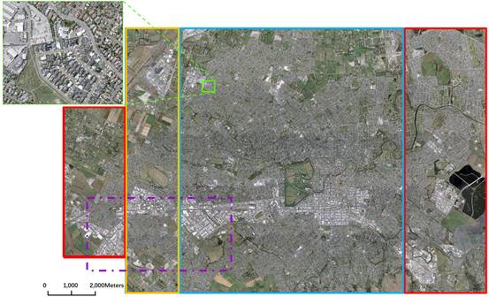
Figure 10: The WHU Aerial Building Dataset in Christchurch, New Zealand. The boxes in blue, yellow and red represent the areas used for creating the training, validation and test sets, respectively.

.

V-D DeepGlobe Building Dataset

The DeepGlobe Building Dataset [72] uses the SpaceNet Building Detection Dataset [71] (Challenge 2 of the SpaceNet Series). This dataset has been used for the DeepGlobe 2018 Satellite Image Understanding Challenge organised as a part of CVPR 2018 Workshops.

The DeepGlobe Dataset for building detection consists of Digital Globe’s WorldView-3 satellite images with 30 cm resolution. The dataset covers 4 different areas of interest (AOIs) with very different landscapes – Vegas, Paris, Shanghai and Khartoum. The training set has 3851 images for Vegas, 1148 images for Paris, 4582 images for Shanghai and 1012 images for Khartoum. In the test set, there are 1282, 381, 1528 and 336 images for Vegas, Paris, Shanghai and Khartoum respectively. Each image is of size $650\times 650$ pixels and covers $200\times 200$ $m^{2}$ area on the ground. Each region consists of high-resolution RGB, panchromatic, and 8-channel lower resolution multi-spectral images. In our experiments, we use pansharpened RGB images. Each image comes with its corresponding geojson file with list of polygons as building instances.

The dataset provides its own evaluation tool to compute F1-score as a performance measure. The F1-score is based on individual building object prediction. Each proposed building is a geospatially defined polygon label representing the footprint of the building. The proposed footprint is considered a “true positive” if the intersection over union (IoU) between the proposed and the ground-truth label is at least 0.5. For each labeled polygon, there can at most one “true positive”. The number of true positives and false positives are counted for all the test images, and the F1-score is computed from this aggregated count.

VI Experimental Settings and Data Preparation

Our entire segmentation pipeline involves the following steps – image preparation, training our GAN based segmentation model using the training and validation datasets, and, finally applying our trained model to predict building masks for the test images. In this paper, we have shown results on 4 different datasets. Due to the diverse characteristics of the datasets and for performing a fair comparison of our algorithm with other state-of-art methods on those datasets, we preprocess our data differently for each dataset. In this section, we first describe our experimental setup. Then, we give detailed explanation of the data processing strategies that we use for each dataset during training and inference.

VI-A Experimental Setup

We have trained our network on four Nvidia GeForce GTX 1080 Ti (11GB) GPUs with images of size $400\times 400$ and batch size of 32. We used the Adam stochastic optimizer with an initial learning rate of 0.0005 and a momentum of 0.9. A poly-iter learning rate [83] with a $power$ of 0.9 was used for 200 epochs. The poly-iter learning rate is calculated as -

$$lr=lr_{0}*\left(1-\frac{i}{T_{i}}\right)^{power}$$ (16)

where $lr$ is the learning rate in the $i^{th}$ iteration, $lr_{0}$ is the initial learning rate and $T_{i}$ is the total numbr of iterations. To avoid overfitting, an L₂ regularization was applied with a weight decay of 0.0002.

VI-B Data Augmentation

During training and inference, we carry out different data augmentation strategies on all four datasets. During training, we perform the following data augmentations – random horizontal flips, random vertical flips, random rotations, and color jitter.

To improve predictive performance of our algorithm, we apply a data augmentation technique during inference – popularly known as Test Time Augmentation (TTA). Specifically, it creates multiple augmented copies of each image in the test set, the model then makes a prediction for each; subsequently, it returns an ensemble of those predictions. We perform 5 different transformations on each test image – flipping the image horizontally and vertically, and rotating the image by $90^{\circ}$, $180^{\circ}$ and $270^{\circ}$. This means we obtain 6 predictions for each image patch. We align these 6 predictions by applying appropriate inverse transformation, and produce the final prediction for each patch by averaging these predictions.

VI-C Creating Training, Test and Validation Datsets

The WHU and Massachusetts datasets provide training, validation and testing subsets.

The DeepGlobe dataset provides training and test subsets. We randomly divide the training set into 80/20 ratio with 80% images in the training dataset and 20% images in the validation dataset. This 80/20 subsets are formed such that the ratios of number of images in each of the 4 AOIs is maintained in the training and validation sets.

For the INRIA dataset, we take a different approach for creating the training, validation and test subsets. This dataset also provides training and testing subsets; however, the regions covered in the training and testing subsets are different. The regions in the training subset includes Austin, Chicago, Kitsap, Vienna and West Tyrol; whereas, the test subset consists of image patches from Bellingham, Bloomington, Innsbruck, San Francisco and East Tyrol. It is evident that this dataset is created with the purpose of investigating how transferable models trained on one set of cities to another set of cities are; to fulfill the same purpose and make our model generalizable to any city in the world, we adopt a k-fold validation technique for training our model, and accordingly, we generate our train, test and validation subsets.

Following the suggestion of the authors of the INRIA dataset paper [15], we create a dataset of 25 images by taking out the first five tiles of each city from the training set (e.g., Austin1-5). In the original dataset paper [15], these 25 images serve as the validation dataset. So, throughout this paper, we have referred to these 25 images as INRIA Validation Dataset. However, most of the state-of-the-art papers have regarded these 25 images as the testing subset and shown inference results on these images. In our paper, we report the performance of our algorithm on the INRIA Validation Dataset (Table V) as well as on the actual test dataset (Table VI).

The rest of the training data now consists of a total of 155 images with 31 images from each region. We split these images into 5 folds, one for each region. We train an ensemble of 5 models - each model being trained on 4 regions and validated on the $5^{th}$ region. Finally, we use an ensemble of 5 models to do prediction on the test images in the INRIA dataset. We compute the integral prediction for an input patch by averaging predictions for each of the models in the ensemble.

(a)

(b)

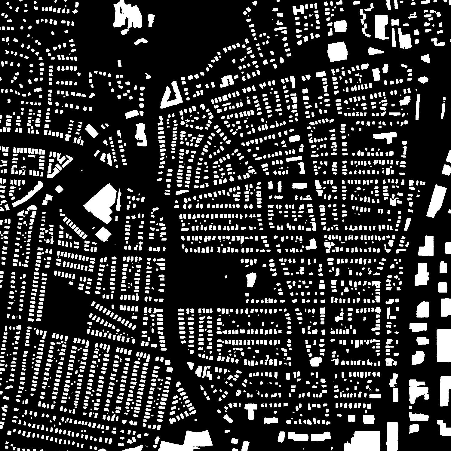
(c)

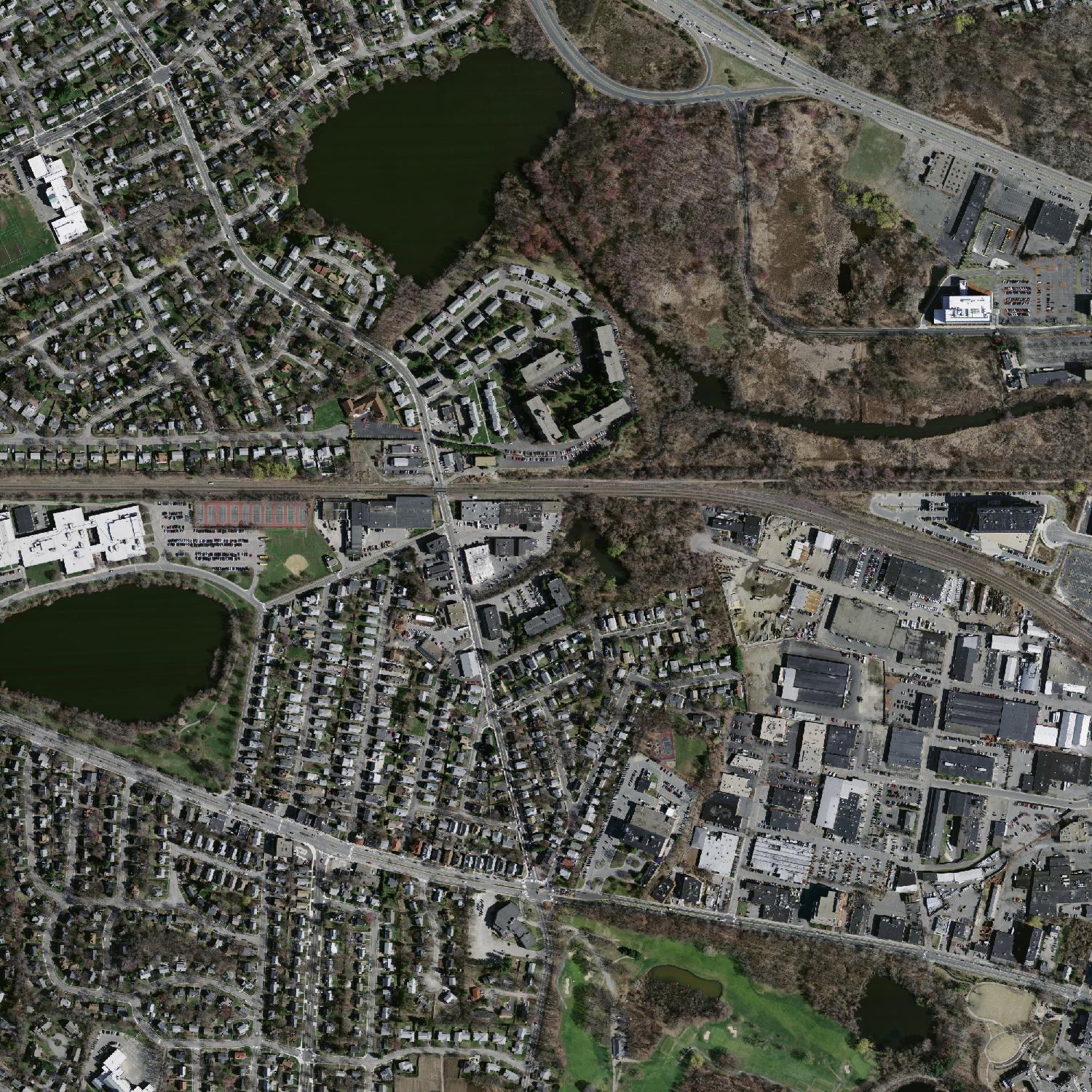
(d)

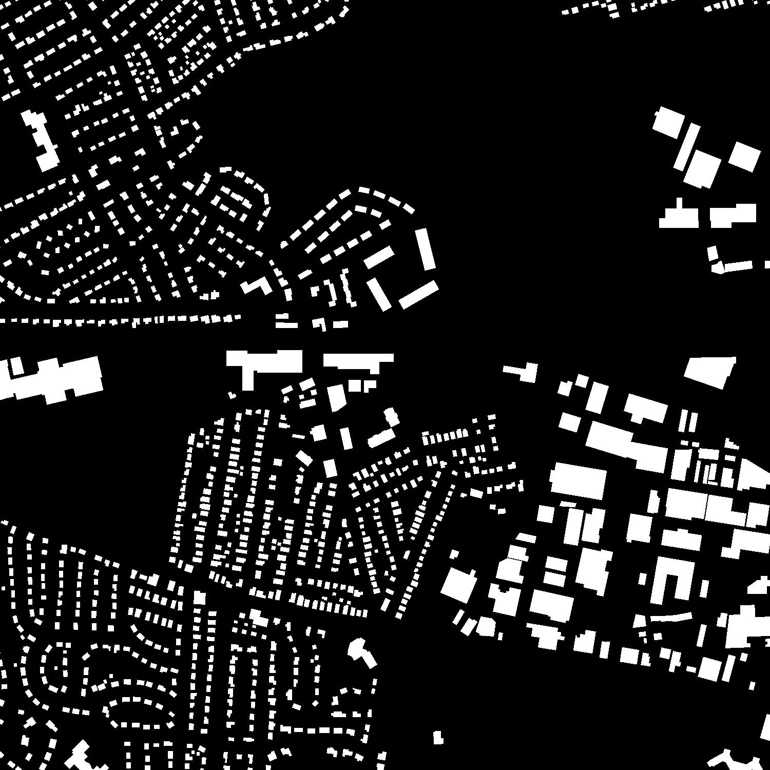
(e)

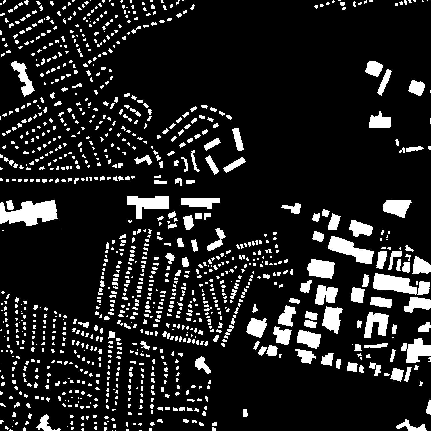
(f)

Figure 11: Results on the Massachusetts Buildings Dataset. Column 1: Input image. Column 2: Ground-truth Label Map. Column 3: Predicted Label Map.

VI-D Patch Extraction and Prediction Fusion

During training, we use image patches of size $400\times 400$. For the INRIA Aerial image Labeling Dataset and the Massachusetts Buildings Dataset, the images provided in the datasets are huge – $5000\times 5000$ for the INRIA dataset and $1500\times 1500$ for the Massachusetts dataset. To fit into the GPU memory, we extract a series of patches, of size $400\times 400$, from the original RGB input images and the corresponding ground-truth label maps. The patches are extracted with 30% overlap so that different parts of the images are seen in multiple patches in different locations. The size of the images in the DeepGlobe dataset is $650\times 650$ and that in the WHU dataset is $512\times 512$. So instead of creating overlapping patches, for these two datasets, we randomly crop patches of size $400\times 400$ as a part of the dynamic data augmentation process.

During inference, memory constraint of a 1080Ti GPU limits the maximum image size to be processed by our algorithm to $2000\times 2000$. We could process whole images from the WHU, Massachusetts and DeepGlobe datasets in one pass. However, to evaluate the performance of our algorithm on the INRIA dataset, we extract patches of size $2000\times 2000$ with 50% overlap, perform segmentation on individual patches and merge the predictions of individual patches into an integral prediction for the whole image. Weighted averaging is applied to merge the predictions in overlapping areas.

VI-E Post-processing

Once we have a prediction map for a whole test image, we binarize it to obtain our final building mask. The optimal threshold for binarization is determined by evaluating the respective metrics on the validation images of a specific dataset.

VII Results

In this section, we present a comparison of our proposed framework with some of the state-of-the work building segmentation approaches.

VII-A Quantitative Evaluation on the Massachusetts Buildings Dataset

Table I presents a relaxed F1-Score (ref. Section V-A) based comparison between the different frameworks on the Massachusetts Buildings Dataset. Our network without TTA achieves a 0.53% performance improvement over the previous best performance [69] with a significantly deeper neural network using 158 layers. The non-TTA version of our algorithm outperforms the shallower version of their network (56 layers) by 0.92% in terms of relaxed F1-score. With TTA, we outperform the previous best model by 1.29%.

Table II demonstrates that our proposed method outperforms other state-of-the-art approaches by at least 2.77% and 3.89% in terms of non-relaxed F1 and IoU scores respectively. Figure 11 presents our semantic segmentation result on $1500\times 1500$ test image patches from the Massachusetts Buildings Dataset.

In Table III, we report the relaxed F1 as well as relaxed IoU scores for our framework and compare the performance of the framework with some benchmark image segmentation approaches when adversarial loss is added to them [10]. Rows 5 and 6 show the performance of our vanilla generator (no attention) and our attention-enhanced generator (with attention) networks. It is clear that the addition of adversarial loss consistently offers better performance across all the metrics, and our attention-guided adversarial model performs best among all the adversarial networks as well.

Method	Relaxed F1
Mnih & Hinton [1]	92.11
Saito et al. [2]	92.30
DeepLab v3+ [10]	92.65
Khalel et al. [4]	96.33
MSMT-Stage-1 [38]	96.04
GAN-SCA [11]	96.36
Building-A-Nets (56 layers) [69]	96.40
Zhang et al. [56]	96.72
Building-A-Nets (158 layers) [69]	96.78
Our Method (no TTA)	97.29
Our Method + TTA	98.03

TABLE I: Relaxed F1-scores of different deep learning based networks on the Massachusetts Buildings Dataset. TTA: Test Time Augmentation. The best results are highlighted in bold.

Method	F1	IoU
DRNet [40]	79.50	66.0
GMEDN [45]	-	70.39
SRI-Net [66]	83.58	71.8
ENRU-Net [12]	84.41	73.02
MSCRF [8]	84.75	71.19
Chen et al. [60]	84.72	73.49
DS-Net2 [64]	84.91	73.79
DS-Net [44]	-	74.43
BMFR-Net [43]	85.14	74.12
BRRNet [41]	85.36	74.46
Liao et al. [42]	85.39	74.51
Zhang et al. [56]	85.49	-
Our Method (no TTA)	86.98	76.97
Our Method + TTA	87.86	77.41

TABLE II: Regular F1 and IoU scores for the state-of-the-art networks on the Massachusetts Buildings Dataset. TTA: Test Time Augmentation. The best results are highlighted in bold.

Method	Relaxed F1	Relaxed IoU
PSPNet	89.52	81.2
PSPNet + adv	91.17	83.78
FC-DenseNet	94.33	89.27
FC-DenseNet + adv	95.59	91.55
Our vanilla Generator	94.11	91.64
Our proposed Generator ($\mathcal{S}$)	96.82	94.79
Our Method ($\mathcal{S}$ + $\mathcal{C}$)	98.03	96.19

TABLE III: Comparison of benchmark image segmentation models with adversarial loss on the Massachusetts Buildings Dataset. adv represents adversarial loss. The scores of our method reflect the results of our algorithm using TTA. The best results are highlighted in bold.

VII-B Quantitative Evaluation on the INRIA Aerial Image Labeling Dataset

Austin
Chicago
Vienna
Kitsap
West Tyrol

figureResults on the INRIA Aerial Image Labeling Validation Dataset. Column 1: Input image. Column 2: Ground-truth Label Map. Column 3: Predicted Label Map. Column 4: Green: True Positives; Blue: False Positives; Red: False Negatives; Grey: True Negatives.

Bellingham	Bloomington	Innsbruck	San Francisco	East Tyrol

figureResults on the INRIA Aerial Image Labeling Test Dataset. Row 1: Input image. Row 2: Predicted Label Map.

Model	Train Cities	Train IoU	Train Acc.	Val. City	Val. IoU	Val. Acc.	INRIA Val. Dataset IoU	INRIA Val. Dataset Acc.
Model 1	Austin, Chicago, Kitsap, W. Tyrol	80.26	96.01	Vienna	78.24	94.13	79.47	96.54
Model 2	Austin, Chicago, Kitsap, Vienna	81.86	96.74	W. Tyrol	79.32	98.29	79.15	97.23
Model 3	Austin, Chicago, W. Tyrol, Vienna	82.93	94.11	Kitsap	70.26	99.22	81.74	97.14
Model 4	Austin, Kitsap, W. Tyrol, Vienna	82.26	95.03	Chicago	72.63	92.46	82.97	95.38
Model 5	Chicago, Kitsap, W. Tyrol, Vienna	79.66	95.29	Austin	80.29	96.78	77.45	96.37

TABLE IV: Comparison of different models in our ensemble of k-fold training on the training and validation subsets of the INRIA Aerial Image Labeling Dataset. Val.: Validation. Acc.: Accuracy

Method	Evaluation Metrics	Austin	Chicago	Kitsap	W. Tyrol	Vienna	Overall
FCN (baseline) [15]	(IoU, Accuracy)	(47.66, 92.22)	(53.62, 88.59)	(33.70, 98.58 )	(46.86, 95.83)	(60.60, 88.72)	(53.82, 92.79)
MLP (baseline) [15]	(IoU, Accuracy)	(61.20, 94.20)	(61.30, 90.43 )	(51.50, 98.92 )	(57.95, 96.66)	(72.13, 91.87 )	(64.67, 94.42)
Mask R-CNN [11]	(IoU, Accuracy)	(65.63, 94.09)	(48.07, 85.56)	(54.38, 97.32)	(70.84, 98.14 )	(64.40, 87.40)	(59.53, 92.49)
MSMT-Stage-1 [38]	(IoU, Accuracy)	(75.39, 95.99)	(67.93, 92.02)	(66.35, 99.24 )	(74.07, 97.78)	(77.12, 92.49)	(73.31, 96.06)
SegNet+Multi-Task Loss [52]	(IoU, Accuracy)	(72.43, 95.71 )	(77.68, 95.60)	(72.28, 95.81)	(64.34, 98.76)	(76.15, 94.48)	(74.49, 96.07)
2-levels U-Nets [4]	(IoU, Accuracy)	(77.29, 96.69)	(68.52, 92.40)	(72.84, 99.25)	(75.38, 98.11)	(78.72, 93.79)	(74.55, 96.05)
U-Net [11]	(IoU, Accuracy)	(79.95, 97.10)	(70.18, 92.67)	(68.56, 99.31)	(76.29, 98.15 )	(79.92, 94.25 )	(76.16, 96.31)
GMEDN [45]	(IoU, Accuracy)	(80.53, 97.19)	(70.42, 92.86)	(68.47, 99.30 )	(75.29, 98.05)	(80.72, 94.54)	(76.69, 96.43)
GAN-SCA [11]	(IoU, Accuracy)	(81.01, 97.26)	(71.73, 93.32)	(68.54, 99.30 )	(78.62, 98.32)	(81.62, 94.84)	(77.75, 96.61)
SEResNeXt101-FPN-CPA [61]	(IoU, Accuracy)	(80.15, 97.18)	(69.54, 92.78)	(70.36, 99.32 )	(80.83, 98.46)	(81.43, 94.67)	(77.29, 96.48)
Building-A-Nets [69]	(IoU, Accuracy)	(80.14, 96.91)	(79.31, 97.06)	(72.77, 96.99 )	(74.55, 93.52)	(75.71, 98.09)	(78.73, 96.71)
Our Method	(IoU, Accuracy)	(83.78, 97.75)	(76.39, 94.83)	(73.25, 99.37)	(85.72, 98.91)	(83.19, 95.09)	(81.28, 97.03)

TABLE V: Comparison of state-of-the-art networks for the INRIA Validation Dataset. The best results are highlighted in bold.

Method	Evaluation Metrics	Bellingham	Bloomington	Innsbruck	San Francisco	East Tyrol	Overall
Building-A-Nets [69]	(IoU, Accuracy)	(65.50, 96.39)	(66.63, 96.85)	(72.59, 96.73)	(76.14, 91.96)	(71.86, 97.48)	(72.36, 95.88)
U-Net-ResNet101 [84]	(IoU, Accuracy)	(69.75, 96.77)	(72.04, 97.13)	(74.64, 96.83)	(74.55, 91.14)	(77.40, 97.92)	(73.91, 95.96)
Zorzi et al. [85]	(IoU, Accuracy)	(70.36, 96.99)	(73.01, 97.36)	(73.34, 96.77)	(75.88, 91.55)	(76.15, 97.84)	(74.40, 96.10)
DS-Net [44]	(IoU, Accuracy)	(71.74, 97.22)	(70.55, 97.27)	(75.44, 97.11)	(77.26, 92.47)	(78.54, 98.10)	(75.52, 96.43)
Zhang et al. [56]	(IoU, Accuracy)	(72.25, 97.25)	(72.49, 97.41)	(75.21, 97.07)	(77.70, 92.54)	(78.06, 98.04)	(75.94, 96.46)
Milosavljevic et al. [86]	(IoU, Accuracy)	(73.90, 97.35)	(72.97, 97.39)	(77.31, 97.32)	(76.46, 92.01)	(80.41, 98.23)	(76.27, 96.46)
E-D-Net [58]	(IoU, Accuracy)	(73.12, 97.22)	(75.58, 97.64)	(77.66, 97.31)	(79.81, 93.26)	(80.61, 98.25)	(78.08, 96.73)
ICT-Net [87]	(IoU, Accuracy)	(74.63, 97.47)	(80.80, 98.18)	(79.50, 97.58)	(81.85, 94.08)	(81.71, 98.39)	(80.32, 97.14)
Our Method	(IoU, Accuracy)	(74.41, 97.03)	(77.29, 97.64)	(76.93, 96.70)	(76.82, 90.49)	(80.11, 98.16)	(77.86, 96.41)

TABLE VI: Comparison of our framework with other state-of-the-art approaches on the test set of the INRIA Aerial Image Labeling Dataset. The best results are highlighted in bold.

As mentioned in Section VI-C, we adopt a k-fold validation strategy for training our network on the INRIA Dataset. In our experiments, k = 5. In Table IV, we report the training as well as the validation IoU and accuracy scores of these 5 models. We also report the overall performance of each model on the INRIA Validation Dataset.

In Table V, we compare the result of our framework with some of the state-of-the-art approaches on the INRIA Validation Dataset. Specifically, we report the IoU and accuracy scores for the different methods. Since the dataset comes with a disproportionately large number of true negatives for the background images, the accuracy numbers achieved with this dataset are generally high, as can be seen by the entries for accuracy in Tables IV-VI. On the other hand, since the IoU metric takes into account both the false alarms and missing detections, we believe that that is a better metric of performance on this dataset.

For the individual cities, as shown in Table V, we have highlighted the highest valued entries for each of the two evaluation metrics. Our network achieves performance improvement of at least 3.42%, 0.56%, 6.05% and 1.92% over Austin, Kitsap, W. Tyrol and Vienna respectively. Our network also gives better accuracy for Austin, Kitsap and W. Tyrol. For Chicago, though our IoU and accuracy are smaller than [69] by 3.82% and 2.35% respectively, overall our algorithm outperforms [69] as well as other state-of-the-art methods by at least 3.24% and 0.33% in terms of IoU and accuracy respectively.

These results show that our network gives consistently good performance over all the cities in the INRIA Validation Dataset, while also yielding the best performance for a subset of the cities. Figures VII-B and VII-B illustrate some of our building segmentation results on the INRIA Validation and Test Dataset.

In Table VI, we compare the performance of our framework with some other state-of-the-art methods on the official INRIA Test Dataset. Though we do not achieve best scores on this subset, our performance is pretty competitive with the state-of-the art methods. Most of the state-of-the-art methods that perform better than us on the INRIA Test Dataset either use pretrained feature extraction networks [88, 89] as backbones or are significantly deeper than our proposed network. This shows effective generalization capability of our network. Notice the drop in both the accuracy and IoU values when applying the trained network to a set of different geographic areas. This is to be expected, since each city has some unique specifics.

VII-C Quantitative Evaluation on the WHU Building Dataset

In Table VII, we report the IoU, precision, recall and F1-scores obtained using our proposed algorithm on the WHU test dataset and compare these scores with some of the best performing state-of-the-art building segmentation approaches. As can be seen from Table VII, our proposed method outperforms the previous best scoring algorithm (ARC-Net [46]) by 0.51%, 0.34%, 0.15% and 0.29% in IoU, precision, recall and F1-score respectively. Figure 12 illustrates some qualitative results of our algorithm on the WHU dataset. The last column in the figure shows the high degree of completeness (i.e. high number of true positives and true negatives, very few false positives and false negatives) in our segmentation results.

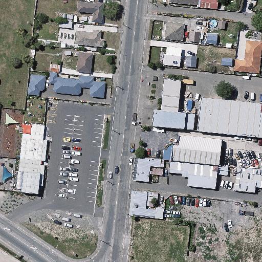
(a)

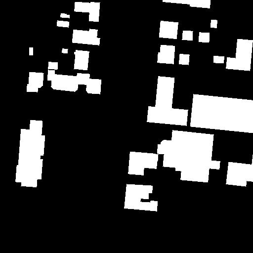
(b)

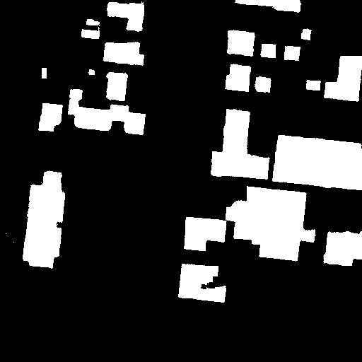
(c)

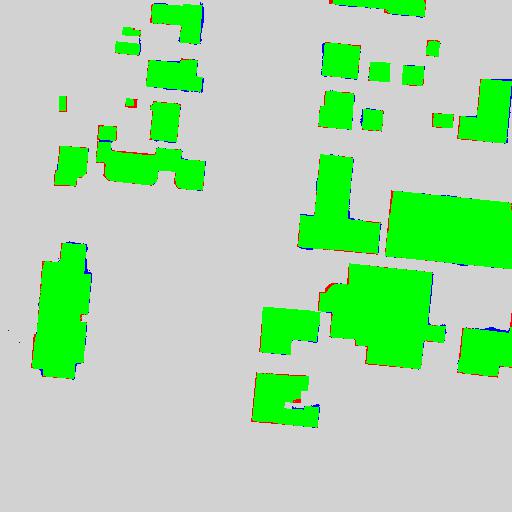
(d)

(e)

(f)

(g)

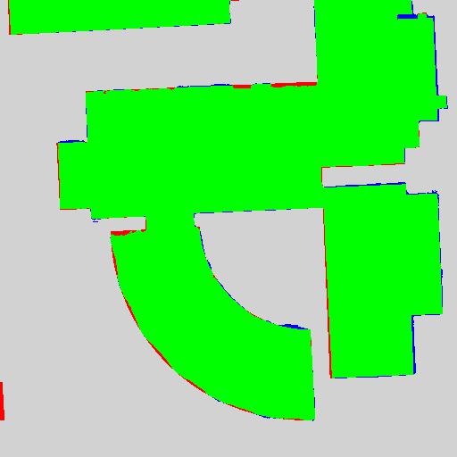
(h)

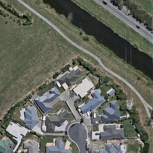
(i)

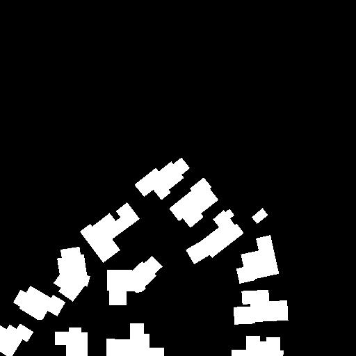
(j)

(k)

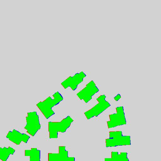
(l)

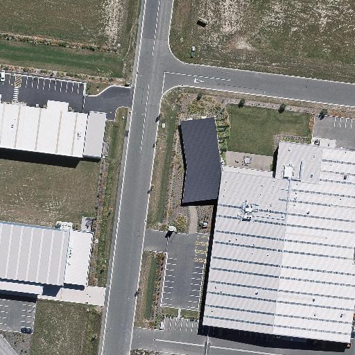
(m)

(n)

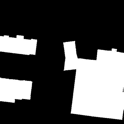
(o)

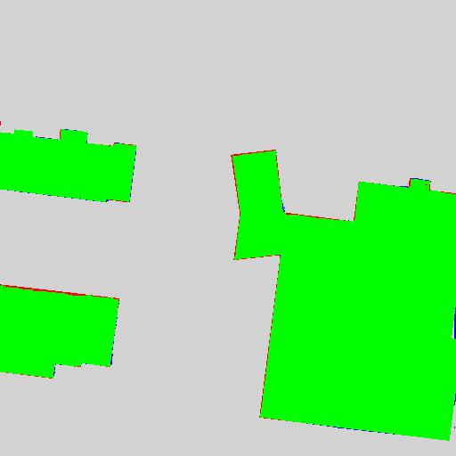
(p)

Figure 12: Results on the WHU Building Dataset. Column 1: Input image. Column 2: Ground-truth Label Map. Column 3: Predicted Label Map. Column 4: Green: True Positives; Blue: False Positives; Red: False Negatives; Grey: True Negatives.

Method	IoU	Precision	Recall	F1
BRRNet [40, 41]	85.9	93.5	91.3	92.4
DRNet [40]	86.0	92.7	92.2	92.5
RefineNet [23, 57]	86.9	93.7	92.3	93.0
PISANet [63]	87.97	94.20	92.94	93.55
SiU-Net [54]	88.4	93.8	93.9	93.8
SRI-Net [66]	89.09	95.21	93.28	94.23
BMFR-Net [43]	89.32	94.31	94.42	94.36
Chen et al. [60]	89.39	93.25	95.56	94.4
Res-U-Net [90]	89.46	94.29	94.53	94.43
HRLinkNetv2 [47]	89.53	94.56	94.40	94.48
DeepLab v3 + [64]	89.61	94.68	92.36	94.52
DE-Net [91]	90.12	95.00	94.60	94.80
DS-Net2 [64]	90.4	94.85	95.06	94.96
He et al. [57]	90.5	95.1	94.9	95.0
MA-FCN [65]	90.7	95.2	95.1	95.15
ARC-Net [46]	91.8	96.4	95.1	95.70
Our Method	92.27	96.73	95.24	95.98

TABLE VII: IoU, Precision, Recall and F1-scores for the state-of-the-art networks on the WHU Building Dataset. The best results are highlighted in bold.

VII-D Quantitative Evaluation on the DeepGlobe Building Dataset

Table VIII illustrates the quantitative performance of our proposed algorithm on the DeepGlobe Building Dataset. Our algorithm achieves F1-scores of 0.896, 0.785, 0.687 and 0.613 over Vegas, Paris, Shanghai and Khartoum respectively. We outperform the previous best (published) F1-scores obtained by TernausNetV2 [5] by 0.56%, 0.51%, 1.03% and 1.65% over Vegas, Paris, Shanghai and Khartoum respectively. Overall, our algorithm outperforms the popular TernausNetV2 network by 0.81%.

To this end, we emphasize the fact that most of the state-of-the-art methods reported in Table VIII use multi-spectral information; whereas our algorithm uses only RGB images for building footprint extraction. We believe incorporating additional spectral information would further improve our algorithm’s segmentation performance.

In addition to the state-of-the-art methods reported in Table VIII, several other papers [92, 56, 59] have shown experimental results on the DeepGlobe Building Dataset. However, they have either chosen their own set of test images or have reported pixel-wise performance scores. In this paper, we report only those works which have reported object-wise performance scores on the test dataset provided by the original DeepGlobe 2018 Competition organizers during the development phase.

Vegas	Paris	Shanghai	Khartoum

figureQualitative results on the test subset of DeepGlobe Building Dataset. Row 1: Input image. Row 2: Predicted Label Map.

Method	Vegas	Paris	Shanghai	Khartoum	Overall
Li et al. [49]	0.886	0.749	0.618	0.554	0.701
Golovanov et al. [48]	-	-	-	-	0.707
Zhao et al. [53]	0.879	0.753	0.642	0.568	0.713
Hamaguchi et al [50]	-	-	-	-	0.726
TernausNetV2 [5]	0.891	0.781	0.680	0.603	0.739
Ali_DI_Deep_Learning∗∗	-	-	-	-	0.749
Our Method	0.896	0.785	0.687	0.613	0.745

TABLE VIII: F1-scores for the state-of-the-art networks on the test subset of DeepGlobe Building Dataset. The best results are highlighted in bold. ^∗∗Leading the DeepGlobe 2018 public leaderboard. Citation is unknown.

Vegas
Paris
Shanghai
Khartoum

figureQualitative results on the validation subset of DeepGlobe Building Dataset. Column 1: Input image. Column 2: Ground-truth Label Map. Column 3: Predicted Label Map. Column 4: Green: True Positives; Blue: False Positives; Red: False Negatives; Grey: True Negatives.

VIII Discussion on the Results and an Ablation Study

The goal of this section is to present a comprehensive overview of the performance of our approach over all four datasets that takes into account the characteristics of each. Subsequently, in a separate subsection, we present an ablation study to verify the effectiveness of the modules for the uncertainty attention and refinement, and also of the deep supervision that is used in our network.

VIII-A Discussion

The results reported in Tables I–IX clearly demonstrate the effectiveness of our proposed algorithm in building segmentation from remotely sensed images. Owing to the Edge Attention Unit and the Hausdorff Loss used in our framework for training, we get accurate building boundaries, as can be seen in Figure 14. The Uncertainty Attention Module helps us to achieve high number of true positives and avoid false alarms (See column 4 of Figure VII-B) by giving more attention to the ambiguous regions of an aerial scene. Further, the Reverse Attention Unit assists us to identify the missing detections by refining the intermediate label maps in a top-down fashion. We also observe significant improvement in the predictive performance of our algorithm when TTA is applied. Tables I and II report scores for both TTA and non-TTA versions of our algorithm. Tables III–IX only report our TTA applied results.

With regard to the INRIA dataset, it is evident from Table V that the performance of our algorithm for the Chicago area is not the best. The buildings in Chicago are located very close to one another, and the network finds it difficult to clearly separate the building boundaries of adjacent buildings. We see the same situation in the San Francisco region – buildings in San Francisco area are also densely packed. Obviously, our framework needs further improvements in separating the buildings that are in close proximity to one another. We believe this issue arises as we use a dilation operator in our edge refinement module. Using an accurate contour extraction algorithm should help us in alleviating this problem.

In general, ground-truth label inconsistencies in the datasets hinder our training process to some extent, and also impact the overall evaluation scores. Specifically, in addition to the building masks being not perfectly aligned to the actual buildings, the Massachusetts Buildings Dataset also contains false labels. Some examples of noisy labels in the Massachusetts Dataset can be seen in column 2 of Figure 13. Moreover, in some of the images, the buildings encompassing playgrounds or parking lots are labeled as a single building instance without capturing the actual shape of the building (column 1 of Figure 13). However, our network identifies the building pixels accurately, as illustrated in row 3 of columns 1 and 2 of Figure 13. Similar noisy labels appear in the INRIA Aerial Image Labeling Dataset. Column 3 of Figure 13 shows an image patch over Vienna where in the ground-truth, smaller building structures close to one-another are clubbed as a one large building. Still, our network accurately predicts each smaller structure. Kitsap County not only has a very sparse distribution of buildings, but mis-labels are also prevalent in the dataset. This severely impacts the evaluation scores. Out of 5 images in the validation dataset, 2 of the images have false building labels. One such example is shown in column 4 of Figure 13. We achieve an IoU of 86.42% as opposed to 73.25% when we leave out those 2 images from the validation set. This kind of mis-labels are found through the training subset as well. However, our network is robust to such mis-labels as evident from the qualitative as well as quantitative results.

Our network yields across-the-board superior performance on the WHU Building Dataset. We believe that the main reason for that is the fact that the ground-truth building maps provided in the WHU dataset are more accurate. We should also mention the relatively low complexity of this dataset in relation to the other three datasets that cover more difficult terrains with high buildings, diverse topography, more occlusions and shadows.

For the DeepGlobe Dataset, our algorithm achieves the best results for Vegas and second highest F1-score for Paris. The images in the Vegas and Paris subsets are mostly collected from residential regions. Unlike the other two cities in the DeepGlobe dataset, the buildings in Vegas and Paris have more unified architectural style. For Shanghai, our proposed method faced difficulty in correctly extracting buildings with green roofs or buildings that are of extremely small size. In Khartoum, there are many building groups, and it is hard to judge, even by the human eye, whether a group of neighboring buildings should be extracted entirely or separately in many regions.

(a)

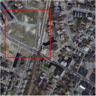
(b)

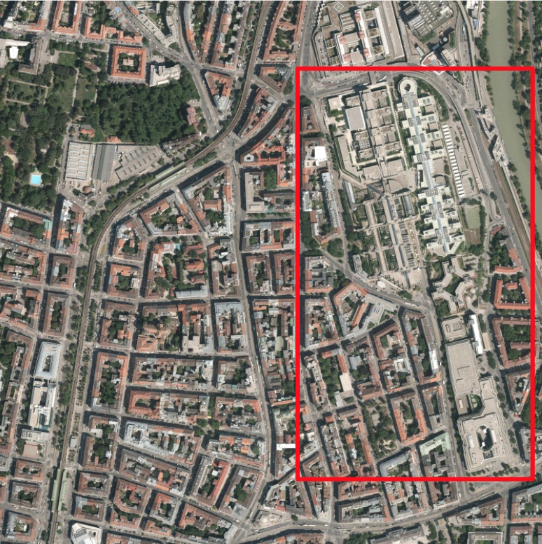
(c)

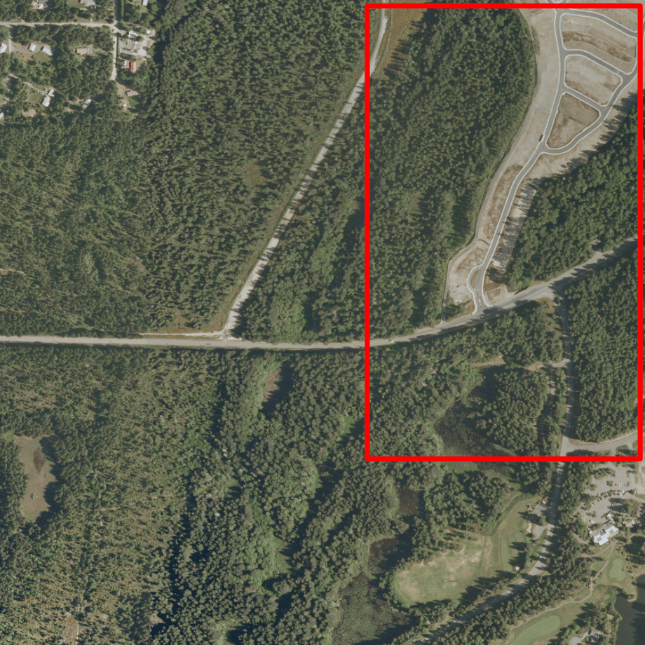
(d)

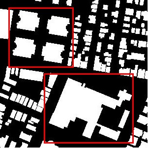
(e)

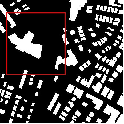
(f)

(g)

(h)

(i)

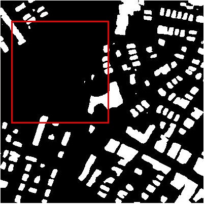
(j)

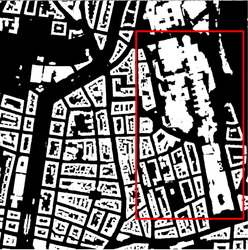
(k)

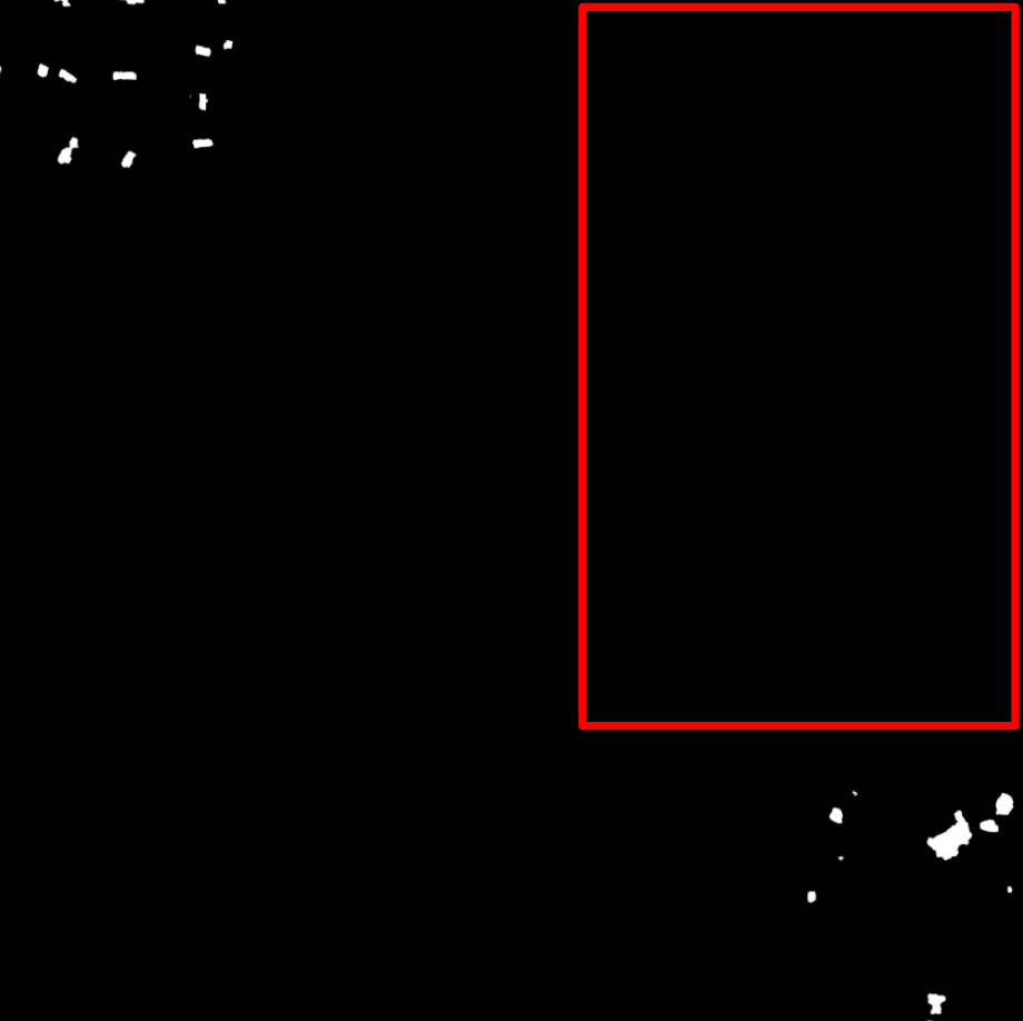
(l)

Figure 13: Noisy labels in the Massachusetts Buildings Dataset (columns 1, 2) and the INRIA Aerial Image Labeling Dataset (columns 3, 4). Row 1: Input Image. Row 2: Ground-truth Labels. Row 3: Predicted Labels. The red boxes represent the areas where noisy labels are present in the ground-truth label maps.

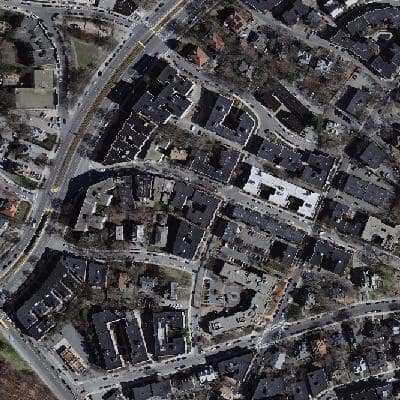
(a)

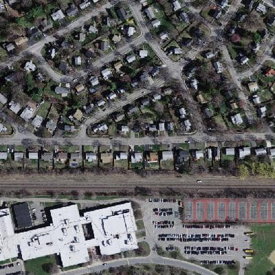
(b)

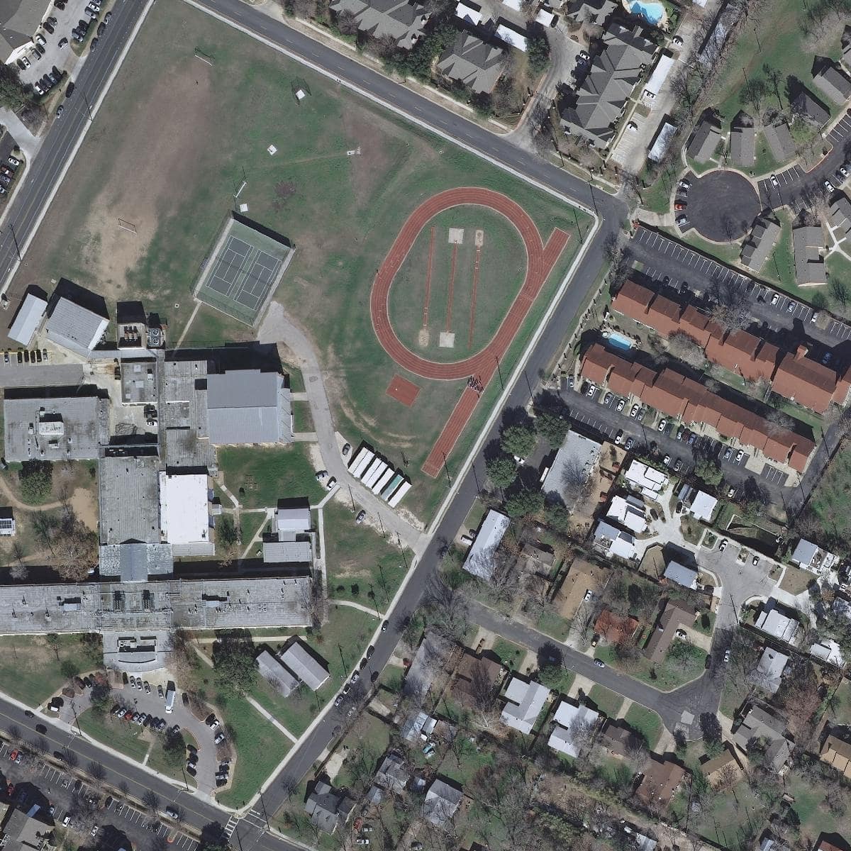
(c)

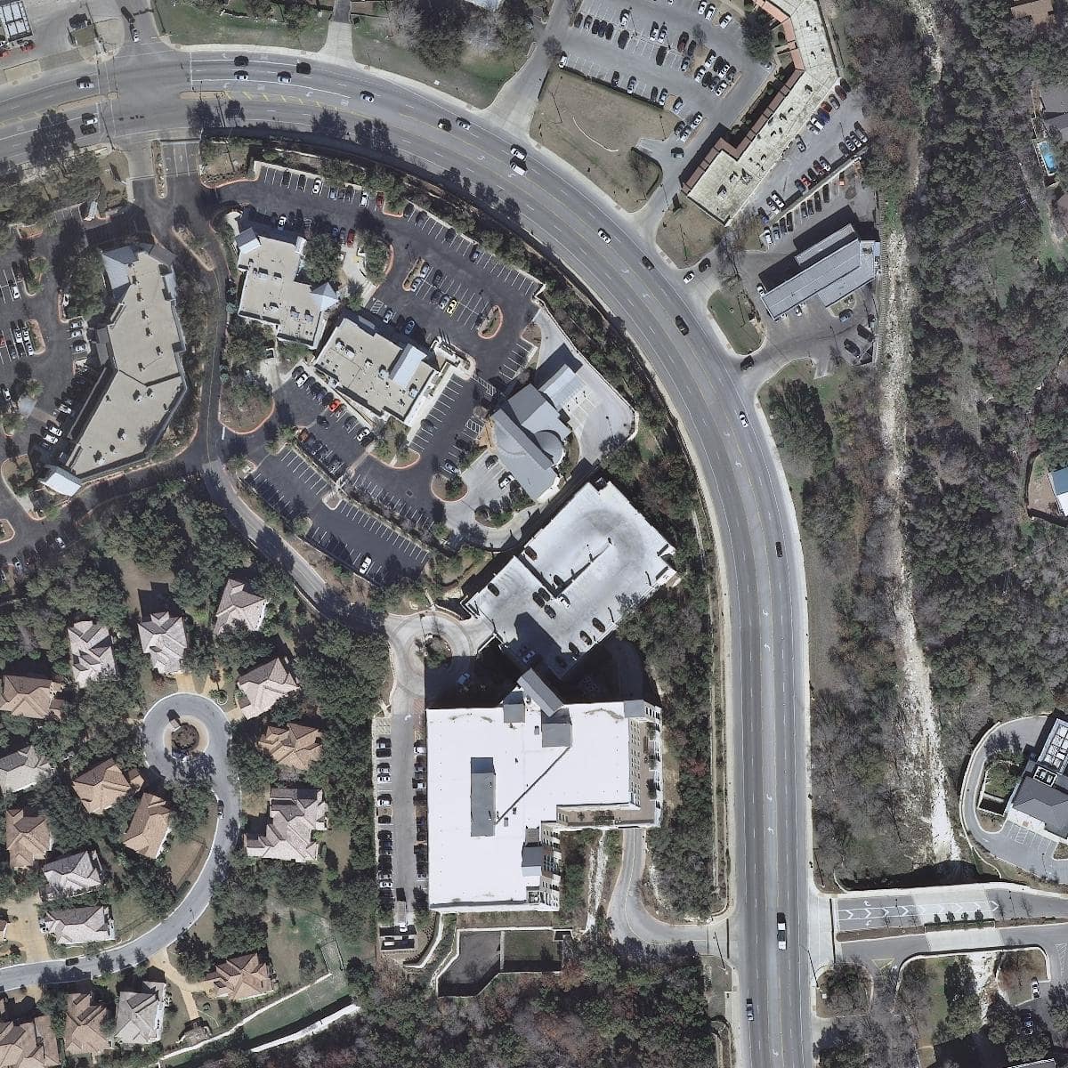
(d)

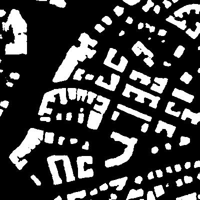
(e)

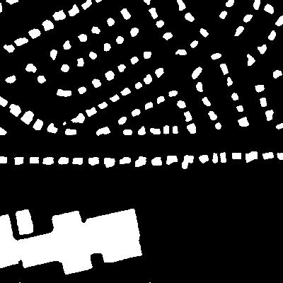
(f)

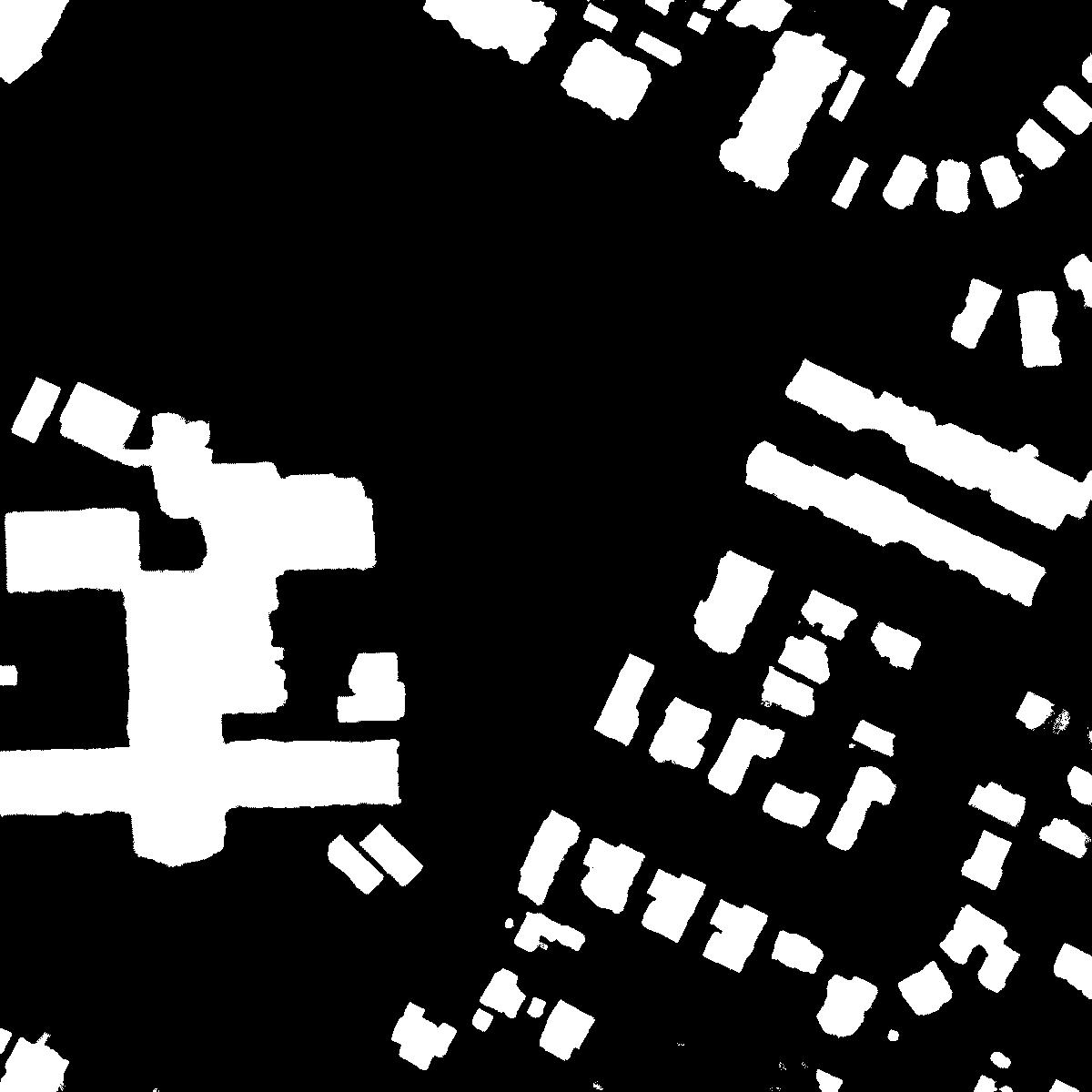
(g)

(h)

Figure 14: Crisp building boundaries using our proposed approach. Row 1: Input Image. Row 2: Predicted Labels.

(a)

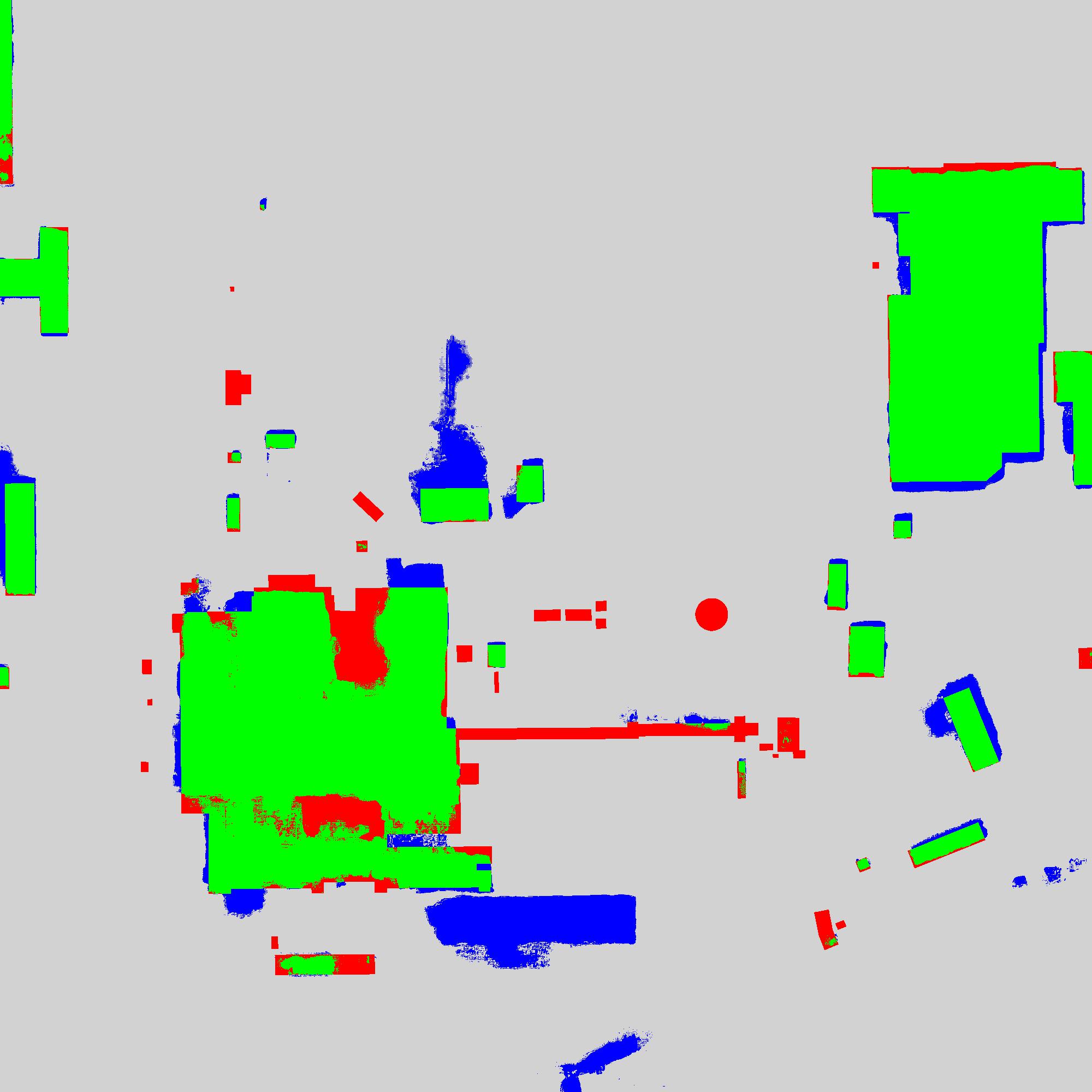
(b)

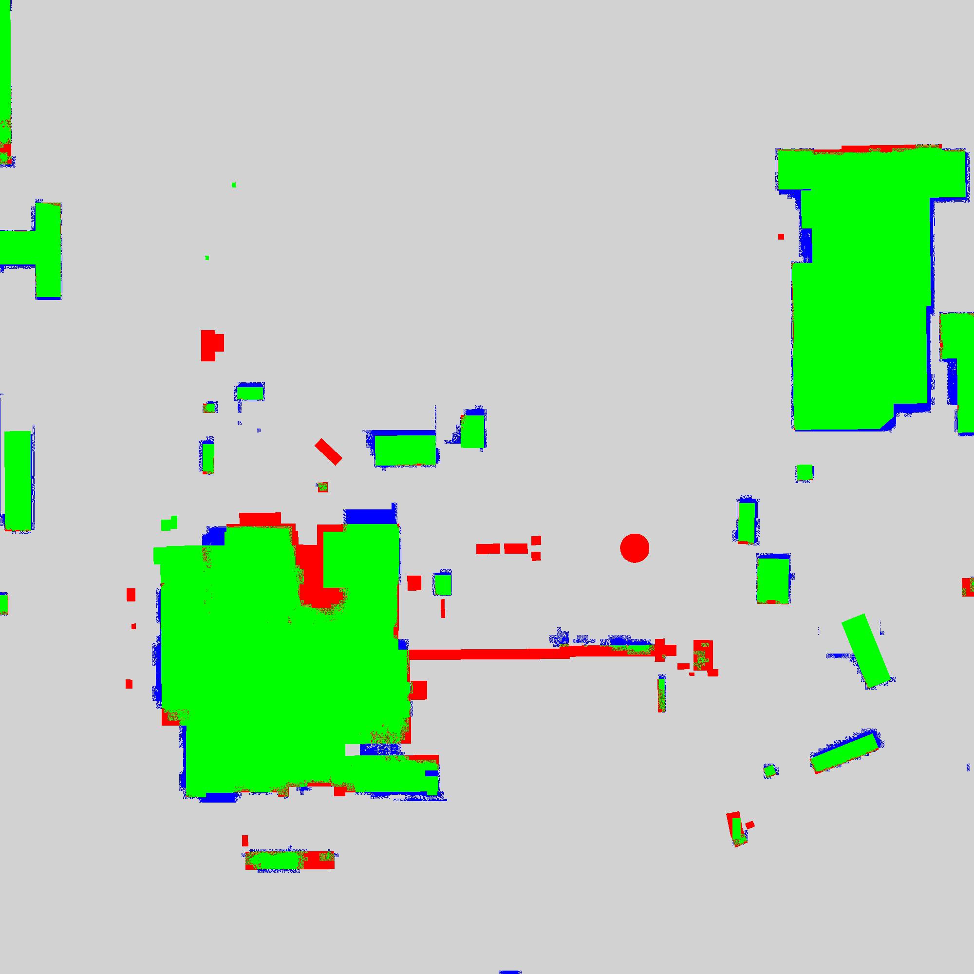
(c)

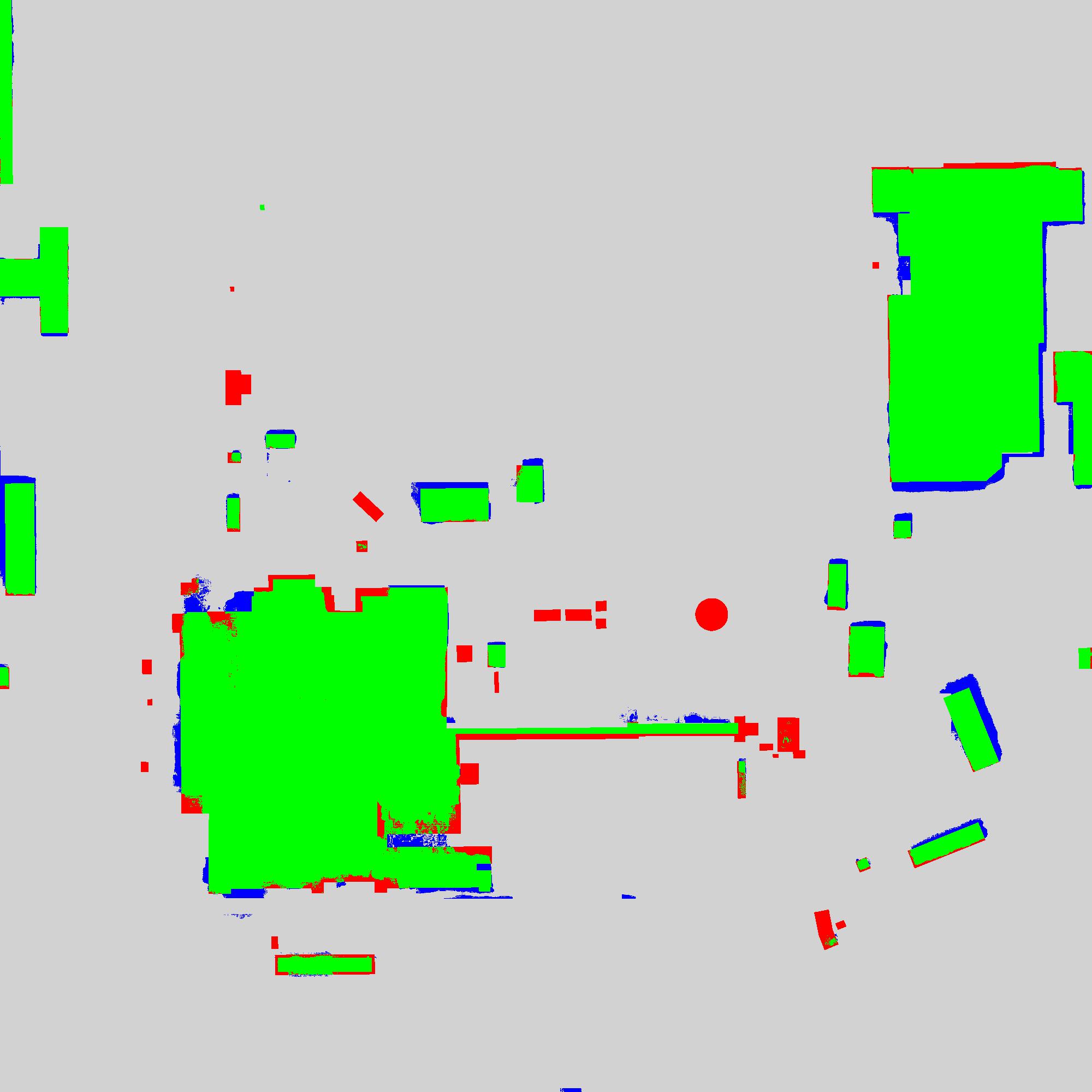
(d)

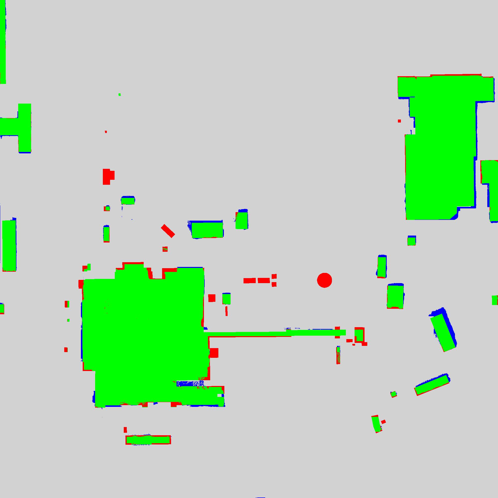
(e)

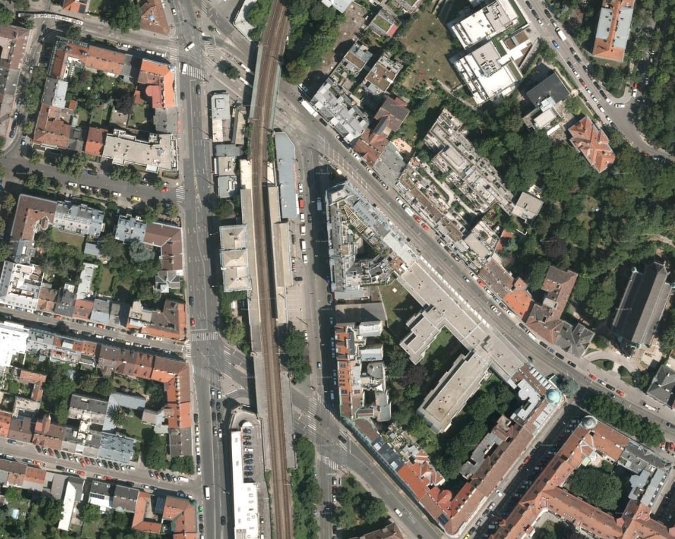
(f)

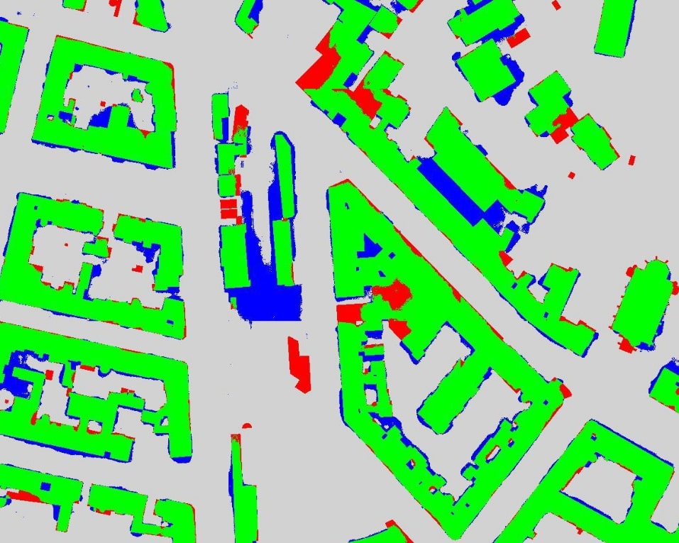
(g)

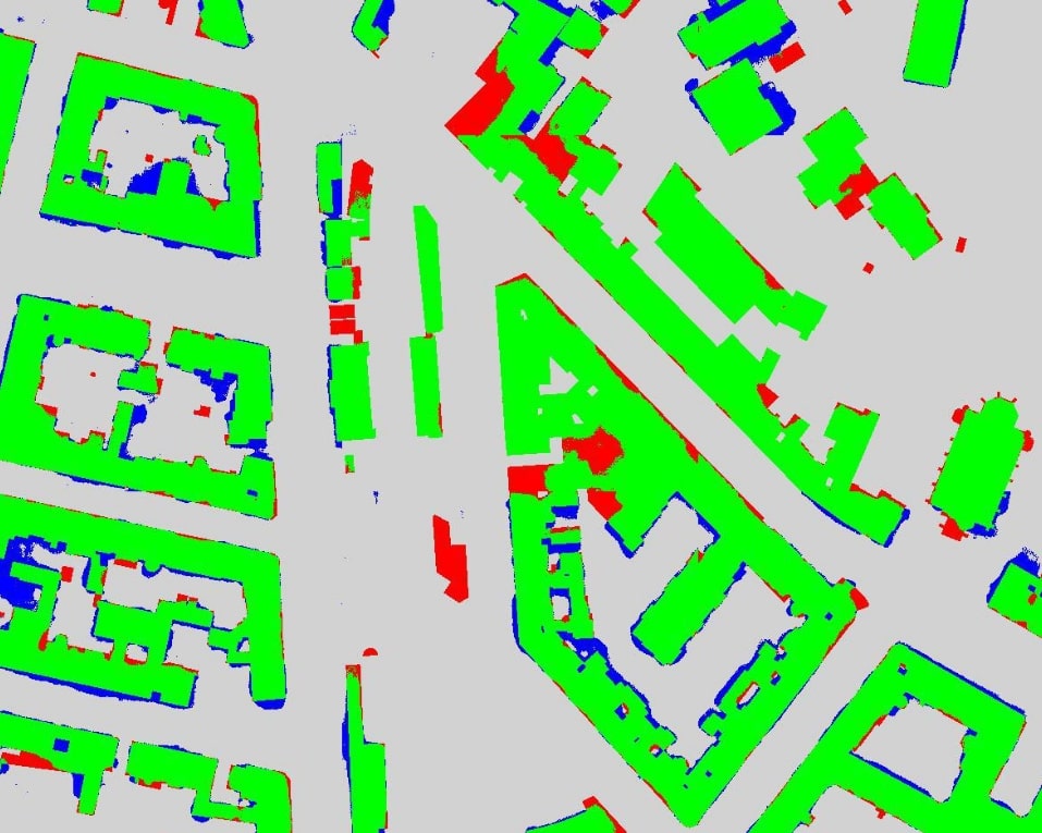
(h)

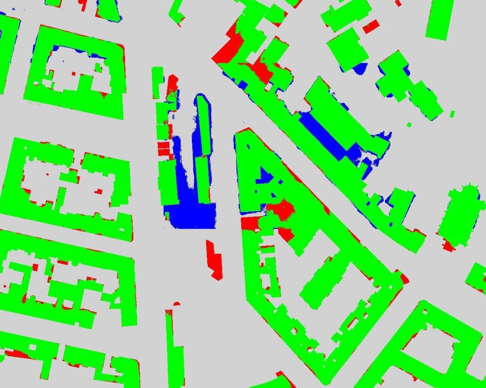
(i)

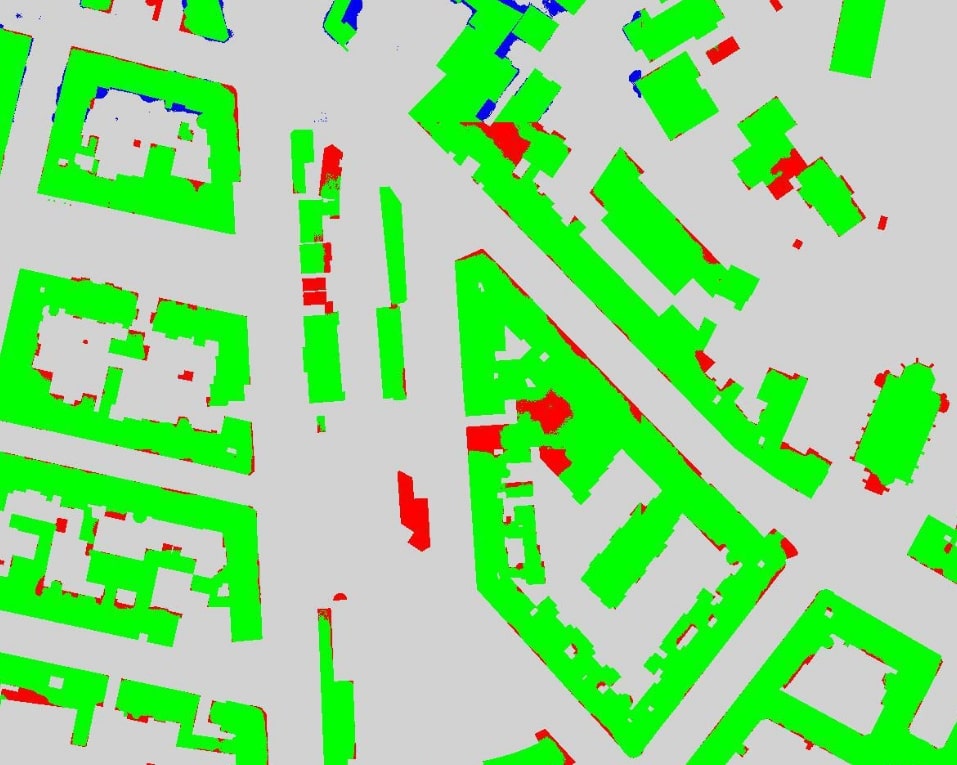
(j)

Figure 15: Ablation study results on Chicago (row 1) and Vienna (row 2) areas of the INRIA Aerial Image Labeling Dataset.   Column 1: Input Image. Column 2: Base GAN Architecture (BGA). Column 3: BGA + Uncertainty Attention Module (UAM). Column 4: BGA + Refinement Module (RM). Column 5: BGA + UAM + RM. All the results are from models trained with deep supervision. Test time augmentation is used for all models. Green: True Positives; Blue: False Positives; Red: False Negatives; Grey: True Negatives.

Method	Austin	Chicago	Kitsap	W. Tyrol	Vienna	Overall
Vanilla Generator (VG)	77.52	69.08	65.69	76.89	79.45	75.31
Base GAN Architecture (BGA) (VG + C)	78.97	70.21	68.07	77.86	79.98	75.93
BGA + DS	80.31	71.77	68.86	79.67	80.18	77.89
BGA + UAM + DS	81.56	73.86	70.64	81.49	81.87	79.36
BGA + RM + DS	80.95	73.12	72.01	82.73	81.13	78.84
BGA + UAM + RM + DS	83.78	76.39	73.25	85.72	83.19	81.28

TABLE IX: Mean IoU scores for the ablation studies performed on the INRIA Validation Dataset. C: Critic, DS: Deep Supervision, UAM: Uncertainty Attention Module, RM: Refinement Module.

VIII-B Ablation Study

To verify the effectiveness of the Uncertainty Attention Module, the Refinement Module, and of the deep supervision technique we have used, we conducted ablation studies using the INRIA Aerial Validation Dataset. We trained 6 different architectures – (a) the vanilla Generator (VG — no attention, deep supervision or critic) (b) the base GAN architecture (BGA — VG + critic); (c) the base GAN architecture with deep supervision (DS); (d) the base GAN architecture with deep supervision and the Uncertainty Attention Module; (e) the base GAN architecture with deep supervision and the Refinement Module; and, (f) the base GAN architecture with Deep Supervision, the Uncertainty Attention Module and the Refinement Module. All the architectures were trained independently with identical training hyper-parameters. Test Time Augmentation is applied while evaluating the performance of the trained models on the validation images. As mentioned in Section VI-C, for the INRIA dataset, all the experiments are conducted using our k-fold validation strategy.

The mean IoU scores for these 6 models are reported in Table IX. On adding the critic, the overall IoU of the Vanilla Generator improves by 0.82%. With deep supervision, we achieve an overall improvement of 2.58% relative to the BGA. The Uncertainty Attention Module and the Refinement Module further improve the mean IoU scores by 1.89% and 1.22% respectively. Finally when we combine all these components, our model outperforms the baseline GAN model by 7.04%.

Figure 15 demonstrates the qualitative performance improvements obtained with the Uncertainty Attention Module and the Refinement Module. In the first row and second column of Figure 15, the large building is labeled incorrectly due to the presence of shadow and absence of global context in the base architecture. However, adding the Uncertainty Attention Module improves the segmentation result, as shown in row 1 and column 3 of Figure 15. Similar results can be seen in row 2, where the base network can not distinguish between roads and buildings since they are similar in color. On the contrary, the model with the Uncertainty Attention Module accurately identifies the building pixels. Column 4 of Figure 15 demonstrates results when we add the Refinement Module to the base GAN architecture. We can observe that the Refinement Module has identified precise building boundaries compared to the base model. When we incorporate both the Uncertainty Attention and the Refinement Modules, we can observe the overall improvement compared to the base module in column 5 of Figure 15.

IX Conclusion

This paper has presented an attention-enhanced residual refining GAN framework for detecting buildings in aerial and satellite images. The proposed approach uses an Uncertainty Attention Module to resolve uncertainties in classification and a Refinement Module to refine the building labels. Specifically, the Refinement Module, whose main job is to refine intermediate prediction maps, uses an Edge Attention Unit to improve the quality of building boundaries and a Reverse Attention Unit to seek missed detections in the intermediate prediction maps. The results demonstrate the effectiveness of our building detection approach even when the buildings are present amidst complex background or are only partly visible due to the presence of shadows. The experimental evaluations that we have conducted in this paper also shows that the proposed method performs equally well on aerial as well as satellite images. In the future, we plan to investigate how to utilize multi-spectral information for further improvement of our network’s capability. Extensive investigations on more diverse datasets (like, roads) have been left for the future.

References

- [1] V. Mnih, “Machine Learning for Aerial Image Labeling,” Ph.D. dissertation, University of Toronto, 2013.
- [2] S. Saito and Y. Aoki, “Building and road detection from large aerial imagery,” in Image Processing: Machine Vision Applications VIII, vol. 9405. International Society for Optics and Photonics, 2015, p. 94050K.
- [3] L.-C. Chen, G. Papandreou, I. Kokkinos, K. Murphy, and A. L. Yuille, “DeepLab: Semantic image segmentation with deep convolutional nets, atrous convolution, and fully connected CRFs,” IEEE transactions on pattern analysis and machine intelligence, vol. 40, no. 4, pp. 834–848, 2017.
- [4] A. Khalel and M. El-Saban, “Automatic pixelwise object labeling for aerial imagery using stacked U-Nets,” arXiv preprint arXiv:1803.04953, 2018.
- [5] V. Iglovikov, S. Seferbekov, A. Buslaev, and A. Shvets, “TernausNetV2: Fully convolutional network for instance segmentation,” in Proceedings of the IEEE Conference on Computer Vision and Pattern Recognition Workshops, 2018, pp. 233–237.
- [6] E. Maggiori, Y. Tarabalka, G. Charpiat, and P. Alliez, “Convolutional neural networks for large-scale remote-sensing image classification,” IEEE Transactions on Geoscience and Remote Sensing, vol. 55, no. 2, pp. 645–657, 2016.
- [7] H. M. Wallach, “Conditional random fields: An introduction,” Technical Reports (CIS), p. 22, 2004.
- [8] Q. Zhu, Z. Li, Y. Zhang, and Q. Guan, “Building extraction from high spatial resolution remote sensing images via multiscale-aware and segmentation-prior conditional random fields,” Remote Sensing, vol. 12, no. 23, p. 3983, 2020.
- [9] B. Cheng, M. D. Collins, Y. Zhu, T. Liu, T. S. Huang, H. Adam, and L.-C. Chen, “Panoptic-DeepLab: A simple, strong, and fast baseline for bottom-up panoptic segmentation,” in Proceedings of the IEEE/CVF Conference on Computer Vision and Pattern Recognition, 2020, pp. 12 475–12 485.
- [10] C. Sebastian, R. Imbriaco, E. Bondarev, and P. H. de With, “Adversarial Loss for Semantic Segmentation of Aerial Imagery,” arXiv preprint arXiv:2001.04269, 2020.
- [11] X. Pan, F. Yang, L. Gao, Z. Chen, B. Zhang, H. Fan, and J. Ren, “Building extraction from high-resolution aerial imagery using a generative adversarial network with spatial and channel attention mechanisms,” Remote Sensing, vol. 11, no. 8, p. 917, 2019.
- [12] S. Wang, X. Hou, and X. Zhao, “Automatic Building Extraction From High-Resolution Aerial Imagery via Fully Convolutional Encoder-Decoder Network With Non-Local Block,” IEEE Access, vol. 8, pp. 7313–7322, 2020.
- [13] I. Goodfellow, J. Pouget-Abadie, M. Mirza, B. Xu, D. Warde-Farley, S. Ozair, A. Courville, and Y. Bengio, “Generative Adversarial Nets,” in Advances in neural information processing systems, 2014, pp. 2672–2680.
- [14] Y. Xue, T. Xu, H. Zhang, L. R. Long, and X. Huang, “Segan: Adversarial network with multi-scale l1 loss for medical image segmentation,” Neuroinformatics, vol. 16, no. 3-4, pp. 383–392, 2018.
- [15] E. Maggiori, Y. Tarabalka, G. Charpiat, and P. Alliez, “Can Semantic Labeling Methods Generalize to Any City? The INRIA Aerial Image Labeling Benchmark,” in IEEE International Geoscience and Remote Sensing Symposium (IGARSS). IEEE, 2017.
- [16] O. Ronneberger, P. Fischer, and T. Brox, “U-Net: Convolutional networks for biomedical image segmentation,” in International Conference on Medical image computing and computer-assisted intervention. Springer, 2015, pp. 234–241.
- [17] A. Tao, K. Sapra, and B. Catanzaro, “Hierarchical multi-scale attention for semantic segmentation,” arXiv preprint arXiv:2005.10821, 2020.
- [18] Y. Yuan, X. Chen, and J. Wang, “Object-contextual representations for semantic segmentation,” arXiv preprint arXiv:1909.11065, 2019.
- [19] X. Li, X. Li, L. Zhang, G. Cheng, J. Shi, Z. Lin, S. Tan, and Y. Tong, “Improving semantic segmentation via decoupled body and edge supervision,” arXiv preprint arXiv:2007.10035, 2020.
- [20] L.-C. Chen, Y. Zhu, G. Papandreou, F. Schroff, and H. Adam, “Encoder-decoder with atrous separable convolution for semantic image segmentation,” in Proceedings of the European conference on computer vision (ECCV), 2018, pp. 801–818.
- [21] H. Zhao, J. Shi, X. Qi, X. Wang, and J. Jia, “Pyramid Scene Parsing Network,” in Proceedings of the IEEE conference on computer vision and pattern recognition, 2017, pp. 2881–2890.
- [22] K. He, G. Gkioxari, P. Dollár, and R. Girshick, “Mask R-CNN,” in Proceedings of the IEEE international conference on computer vision, 2017, pp. 2961–2969.
- [23] G. Lin, A. Milan, C. Shen, and I. Reid, “RefineNet: Multi-path refinement networks for high-resolution semantic segmentation,” in Proceedings of the IEEE conference on computer vision and pattern recognition, 2017, pp. 1925–1934.
- [24] H. Wu, J. Zhang, K. Huang, K. Liang, and Y. Yu, “FastFCN: Rethinking dilated convolution in the backbone for semantic segmentation,” arXiv preprint arXiv:1903.11816, 2019.
- [25] J. Fu, J. Liu, H. Tian, Y. Li, Y. Bao, Z. Fang, and H. Lu, “Dual attention network for scene segmentation,” in Proceedings of the IEEE/CVF Conference on Computer Vision and Pattern Recognition, 2019, pp. 3146–3154.
- [26] F. Yu and V. Koltun, “Multi-scale context aggregation by dilated convolutions,” arXiv preprint arXiv:1511.07122, 2015.
- [27] Y.-J. Zhang, “An overview of image and video segmentation in the last 40 years,” Advances in Image and Video Segmentation, pp. 1–16, 2006.
- [28] T. Lindeberg and M.-X. Li, “Segmentation and classification of edges using minimum description length approximation and complementary junction cues,” Computer Vision and Image Understanding, vol. 67, no. 1, pp. 88–98, 1997.
- [29] S. S. Al-Amri, N. Kalyankar, and S. Khamitkar, “Image segmentation by using edge detection,” International journal on computer science and engineering, vol. 2, no. 3, pp. 804–807, 2010.
- [30] M. R. Khokher, A. Ghafoor, and A. M. Siddiqui, “Image segmentation using multilevel graph cuts and graph development using fuzzy rule-based system,” IET image processing, vol. 7, no. 3, pp. 201–211, 2013.
- [31] R. Muthukrishnan and M. Radha, “Edge detection techniques for image segmentation,” International Journal of Computer Science & Information Technology, vol. 3, no. 6, p. 259, 2011.
- [32] S. Angelina, L. P. Suresh, and S. K. Veni, “Image segmentation based on genetic algorithm for region growth and region merging,” in 2012 international conference on computing, electronics and electrical technologies (ICCEET). IEEE, 2012, pp. 970–974.
- [33] H. G. Kaganami and Z. Beiji, “Region-based segmentation versus edge detection,” in 2009 Fifth International Conference on Intelligent Information Hiding and Multimedia Signal Processing. IEEE, 2009, pp. 1217–1221.
- [34] M. Yambal and H. Gupta, “Image segmentation using fuzzy C-means clustering: a survey,” International Journal of Advanced Research in Computer and Communication Engineering, vol. 2, no. 7, pp. 2927–2929, 2013.
- [35] V. K. Dehariya, S. K. Shrivastava, and R. Jain, “Clustering of image data set using k-means and fuzzy k-means algorithms,” in 2010 International Conference on Computational Intelligence and Communication Networks. IEEE, 2010, pp. 386–391.
- [36] S. Beucher et al., “The watershed transformation applied to image segmentation,” Scanning microscopy-supplement-, pp. 299–299, 1992.
- [37] J. Lin, W. Jing, H. Song, and G. Chen, “ESFNet: Efficient network for building extraction from high-resolution aerial images,” IEEE Access, vol. 7, pp. 54 285–54 294, 2019.
- [38] A. Marcu, D. Costea, E. Slusanschi, and M. Leordeanu, “A multi-stage multi-task neural network for aerial scene interpretation and geolocalization,” arXiv preprint arXiv:1804.01322, 2018.
- [39] A. E. Marcu and M. Leordeanu, “Object Contra Context: Dual local-global semantic segmentation in aerial images,” in AAAI Workshops, 2017.
- [40] M. Chen, J. Wu, L. Liu, W. Zhao, F. Tian, Q. Shen, B. Zhao, and R. Du, “DR-Net: An improved network for building extraction from high resolution remote sensing image,” Remote Sensing, vol. 13, no. 2, p. 294, 2021.
- [41] Z. Shao, P. Tang, Z. Wang, N. Saleem, S. Yam, and C. Sommai, “BRRNet: A fully convolutional neural network for automatic building extraction from high-resolution remote sensing images,” Remote Sensing, vol. 12, no. 6, p. 1050, 2020.
- [42] C. Liao, H. Hu, H. Li, X. Ge, M. Chen, C. Li, and Q. Zhu, “Joint Learning of Contour and Structure for Boundary-Preserved Building Extraction,” Remote Sensing, vol. 13, no. 6, p. 1049, 2021.
- [43] S. Ran, X. Gao, Y. Yang, S. Li, G. Zhang, and P. Wang, “Building Multi-Feature Fusion Refined Network for Building Extraction from High-Resolution Remote Sensing Images,” Remote Sensing, vol. 13, no. 14, p. 2794, 2021.
- [44] Y. Liao, H. Zhang, G. Yang, and L. Zhang, “Learning Discriminative Global and Local Features for Building Extraction from Aerial Images,” in IGARSS 2020-2020 IEEE International Geoscience and Remote Sensing Symposium. IEEE, 2020, pp. 1821–1824.
- [45] J. Ma, L. Wu, X. Tang, F. Liu, X. Zhang, and L. Jiao, “Building extraction of aerial images by a global and multi-scale encoder-decoder network,” Remote Sensing, vol. 12, no. 15, p. 2350, 2020.
- [46] Y. Liu, J. Zhou, W. Qi, X. Li, L. Gross, Q. Shao, Z. Zhao, L. Ni, X. Fan, and Z. Li, “ARC-Net: An efficient network for building extraction from high-resolution aerial images,” IEEE Access, vol. 8, pp. 154 997–155 010, 2020.
- [47] M. Wu, Z. Shu, J. Zhang, and X. Hu, “HRLINKNet: LinkNet with High-Resolution Representation for High-Resolution Satellite Imagery,” in 2021 IEEE International Geoscience and Remote Sensing Symposium IGARSS. IEEE, 2021, pp. 2504–2507.
- [48] S. Golovanov, R. Kurbanov, A. Artamonov, A. Davydow, and S. Nikolenko, “Building detection from satellite imagery using a composite loss function,” in Proceedings of the IEEE Conference on Computer Vision and Pattern Recognition Workshops, 2018, pp. 229–232.
- [49] W. Li, C. He, J. Fang, and H. Fu, “Semantic segmentation based building extraction method using multi-source GIS map datasets and satellite imagery,” in Proceedings of the IEEE Conference on Computer Vision and Pattern Recognition Workshops, 2018, pp. 238–241.
- [50] R. Hamaguchi and S. Hikosaka, “Building Detection From Satellite Imagery Using Ensemble of Size-Specific Detectors,” in Proceedings of the IEEE Conference on Computer Vision and Pattern Recognition (CVPR) Workshops, June 2018.
- [51] J. Hu, L. Li, Y. Lin, F. Wu, and J. Zhao, “Light-Weight Edge Enhanced Network for On-orbit Semantic Segmentation,” in International Conference on Artificial Neural Networks. Springer, 2019, pp. 321–333.
- [52] B. Bischke, P. Helber, J. Folz, D. Borth, and A. Dengel, “Multi-task learning for segmentation of building footprints with deep neural networks,” in 2019 IEEE International Conference on Image Processing (ICIP). IEEE, 2019, pp. 1480–1484.
- [53] K. Zhao, J. Kang, J. Jung, and G. Sohn, “Building Extraction From Satellite Images Using Mask R-CNN With Building Boundary Regularization,” in Proceedings of the IEEE Conference on Computer Vision and Pattern Recognition (CVPR) Workshops, June 2018.
- [54] S. Ji, S. Wei, and M. Lu, “Fully convolutional networks for multisource building extraction from an open aerial and satellite imagery data set,” IEEE Transactions on Geoscience and Remote Sensing, vol. 57, no. 1, pp. 574–586, 2018.
- [55] L. Mou, Y. Hua, and X. X. Zhu, “A relation-augmented fully convolutional network for semantic segmentation in aerial scenes,” in Proceedings of the IEEE/CVF Conference on Computer Vision and Pattern Recognition, 2019, pp. 12 416–12 425.
- [56] H. Zhang, Y. Liao, H. Yang, G. Yang, and L. Zhang, “A Local-Global Dual-Stream Network for Building Extraction From Very-High-Resolution Remote Sensing Images,” IEEE Transactions on Neural Networks and Learning Systems, 2020.
- [57] S. He and W. Jiang, “Boundary-Assisted Learning for Building Extraction from Optical Remote Sensing Imagery,” Remote Sensing, vol. 13, no. 4, p. 760, 2021.
- [58] Y. Zhu, Z. Liang, J. Yan, G. Chen, and X. Wang, “ED-Net: Automatic Building Extraction From High-Resolution Aerial Images With Boundary Information,” IEEE Journal of Selected Topics in Applied Earth Observations and Remote Sensing, vol. 14, pp. 4595–4606, 2021.
- [59] H. Jung, H.-S. Choi, and M. Kang, “Boundary Enhancement Semantic Segmentation for Building Extraction From Remote Sensed Image,” IEEE Transactions on Geoscience and Remote Sensing, 2021.
- [60] Z. Chen, D. Li, W. Fan, H. Guan, C. Wang, and J. Li, “Self-attention in reconstruction bias U-Net for semantic segmentation of building rooftops in optical remote sensing images,” Remote Sensing, vol. 13, no. 13, p. 2524, 2021.
- [61] C. Sebastian, R. Imbriaco, E. Bondarev, and P. H. de With, “Contextual pyramid attention network for building segmentation in aerial imagery,” arXiv preprint arXiv:2004.07018, 2020.
- [62] Z. Zhang, C. Zhang, and W. Li, “Semantic Segmentation of Urban Buildings from VHR Remotely Sensed Imagery Using Attention-Based CNN,” in IGARSS 2020-2020 IEEE International Geoscience and Remote Sensing Symposium. IEEE, 2020, pp. 1833–1836.
- [63] D. Zhou, G. Wang, G. He, T. Long, R. Yin, Z. Zhang, S. Chen, and B. Luo, “Robust Building Extraction for High Spatial Resolution Remote Sensing Images with Self-Attention Network,” Sensors, vol. 20, no. 24, p. 7241, 2020.
- [64] H. Guo, X. Su, S. Tang, B. Du, and L. Zhang, “Scale-Robust Deep-Supervision Network for Mapping Building Footprints From High-Resolution Remote Sensing Images,” IEEE Journal of Selected Topics in Applied Earth Observations and Remote Sensing, vol. 14, pp. 10 091–10 100, 2021.
- [65] S. Wei, S. Ji, and M. Lu, “Toward automatic building footprint delineation from aerial images using CNN and regularization,” IEEE Transactions on Geoscience and Remote Sensing, vol. 58, no. 3, pp. 2178–2189, 2019.
- [66] P. Liu, X. Liu, M. Liu, Q. Shi, J. Yang, X. Xu, and Y. Zhang, “Building footprint extraction from high-resolution images via spatial residual inception convolutional neural network,” Remote Sensing, vol. 11, no. 7, p. 830, 2019.
- [67] B. Comandur and A. C. Kak, “Semantic Labeling of Large-Area Geographic Regions Using Multiview and Multidate Satellite Images and Noisy OSM Training Labels,” IEEE Journal of Selected Topics in Applied Earth Observations and Remote Sensing, vol. 14, pp. 4573–4594, 2021.
- [68] N. Weir, D. Lindenbaum, A. Bastidas, A. V. Etten, S. McPherson, J. Shermeyer, V. Kumar, and H. Tang, “SpaceNet MVOI: A Multi-view Overhead Imagery Dataset,” in Proceedings of the IEEE/CVF International Conference on Computer Vision (ICCV), October 2019.
- [69] X. Li, X. Yao, and Y. Fang, “Building-A-Nets: Robust building extraction from high-resolution remote sensing images with adversarial networks,” IEEE Journal of Selected Topics in Applied Earth Observations and Remote Sensing, vol. 11, no. 10, pp. 3680–3687, 2018.
- [70] A. Abdollahi, B. Pradhan, S. Gite, and A. Alamri, “Building Footprint Extraction from High Resolution Aerial Images Using Generative Adversarial Network (GAN) Architecture,” IEEE Access, vol. 8, pp. 209 517–209 527, 2020.
- [71] A. Van Etten, D. Lindenbaum, and T. M. Bacastow, “SpaceNet: A remote sensing dataset and challenge series,” arXiv preprint arXiv:1807.01232, 2018.
- [72] I. Demir, K. Koperski, D. Lindenbaum, G. Pang, J. Huang, S. Basu, F. Hughes, D. Tuia, and R. Raskar, “DeepGlobe 2018: A Challenge to Parse the Earth Through Satellite Images,” in The IEEE Conference on Computer Vision and Pattern Recognition (CVPR) Workshops, June 2018.
- [73] J.-Y. Sun, S.-W. Kim, S.-W. Lee, Y.-W. Kim, and S.-J. Ko, “Reverse and Boundary Attention Network for Road Segmentation,” in Proceedings of the IEEE International Conference on Computer Vision Workshops, 2019, pp. 0–0.
- [74] J.-Y. Sun, S.-W. Jung, and S.-J. Ko, “Lightweight Prediction and Boundary Attention-Based Semantic Segmentation for Road Scene Understanding,” IEEE Access, vol. 8, pp. 108 449–108 460, 2020.
- [75] S. Chen, X. Tan, B. Wang, and X. Hu, “Reverse attention for salient object detection,” in Proceedings of the European Conference on Computer Vision (ECCV), 2018, pp. 234–250.
- [76] W. Gao, X. Zhang, L. Yang, and H. Liu, “An improved Sobel edge detection,” in 2010 3rd International conference on computer science and information technology, vol. 5. IEEE, 2010, pp. 67–71.
- [77] Y. Pang, Y. Li, J. Shen, and L. Shao, “Towards bridging semantic gap to improve semantic segmentation,” in Proceedings of the IEEE/CVF International Conference on Computer Vision, 2019, pp. 4230–4239.
- [78] L. Wang, C.-Y. Lee, Z. Tu, and S. Lazebnik, “Training deeper convolutional networks with deep supervision,” arXiv preprint arXiv:1505.02496, 2015.
- [79] C.-Y. Lee, S. Xie, P. Gallagher, Z. Zhang, and Z. Tu, “Deeply-Supervised Nets,” in Artificial intelligence and statistics. PMLR, 2015, pp. 562–570.
- [80] S. Xie and Z. Tu, “Holistically-Nested Edge Detection,” in Proceedings of the IEEE international conference on computer vision, 2015, pp. 1395–1403.
- [81] Q. Dou, L. Yu, H. Chen, Y. Jin, X. Yang, J. Qin, and P.-A. Heng, “3D deeply supervised network for automated segmentation of volumetric medical images,” Medical image analysis, vol. 41, pp. 40–54, 2017.
- [82] D. Karimi and S. E. Salcudean, “Reducing the Hausdorff distance in medical image segmentation with convolutional neural networks,” IEEE Transactions on medical imaging, vol. 39, no. 2, pp. 499–513, 2019.
- [83] P. Mishra and K. Sarawadekar, “Polynomial learning rate policy with warm restart for deep neural network,” in TENCON 2019-2019 IEEE Region 10 Conference (TENCON). IEEE, 2019, pp. 2087–2092.
- [84] N. Girard, D. Smirnov, J. Solomon, and Y. Tarabalka, “Polygonal Building Extraction by Frame Field Learning,” in Proceedings of the IEEE/CVF Conference on Computer Vision and Pattern Recognition, 2021, pp. 5891–5900.
- [85] S. Zorzi, K. Bittner, and F. Fraundorfer, “Machine-learned regularization and polygonization of building segmentation masks,” in 2020 25th International Conference on Pattern Recognition (ICPR). IEEE, 2021, pp. 3098–3105.
- [86] A. Milosavljević, “Automated processing of remote sensing imagery using deep semantic segmentation: A building footprint extraction case,” ISPRS International Journal of Geo-Information, vol. 9, no. 8, p. 486, 2020.
- [87] B. Chatterjee and C. Poullis, “Semantic segmentation from remote sensor data and the exploitation of latent learning for classification of auxiliary tasks,” Computer Vision and Image Understanding, vol. 210, p. 103251, 2021.
- [88] A. Krizhevsky, I. Sutskever, and G. E. Hinton, “ImageNet classification with deep convolutional neural networks,” Advances in neural information processing systems, vol. 25, pp. 1097–1105, 2012.
- [89] K. Simonyan and A. Zisserman, “Very deep convolutional networks for large-scale image recognition,” arXiv preprint arXiv:1409.1556, 2014.
- [90] Y. Xu, L. Wu, Z. Xie, and Z. Chen, “Building extraction in very high resolution remote sensing imagery using deep learning and guided filters,” Remote Sensing, vol. 10, no. 1, p. 144, 2018.
- [91] H. Liu, J. Luo, B. Huang, X. Hu, Y. Sun, Y. Yang, N. Xu, and N. Zhou, “DE-Net: Deep encoding network for building extraction from high-resolution remote sensing imagery,” Remote Sensing, vol. 11, no. 20, p. 2380, 2019.
- [92] J. Liu, Z. Wang, and K. Cheng, “An improved algorithm for semantic segmentation of remote sensing images based on DeepLabV3+,” in Proceedings of the 5th International Conference on Communication and Information Processing, 2019, pp. 124–128.