Controlling Valley-Polarisation in Graphene via Tailored Light Pulses

Abstract

Analogous to charge and spin, electrons in solids endows an additional degree of freedom: the valley pseudospin. Two-dimensional hexagonal materials such as graphene exhibit two valleys, labelled as $\mathbf{K}$ and $\mathbf{K}^{\prime}$. These two valleys have the potential to realise logical operations in two-dimensional materials. Obtaining the desired control over valley polarisation between the two valleys is a prerequisite for the logical operations. Recently, it was shown that two counter-rotating circularly polarised laser pulses can induce a significant valley-polarisation in graphene. The main focus of the present work is to optimise the valley polarisation in monolayer graphene by controlling different laser parameters, such as wavelength, intensity ratio, frequency ratio and sub-cycle phase in two counter-rotating circularly polarised laser setup. Moreover, an alternate approach, based on single or few-cycle linearly polarised laser pulse, is also explored to induce significant valley polarisation in graphene. Our work could help experimentalists to choose a suitable method with optimised parameter space to obtain the desired control over valley polarisation in monolayer graphene.

I Introduction

Graphene is a centrosymmetric two-dimensional material with zero bandgap novoselov2005two . Massless Dirac equation is used to describe the charge carriers with exceptional transport properties, which have lead to the proliferation of interesting physical phenomena, such as topological superconductivity or anomalous integer quantum Hall effect neto2009electronic ; geim2009graphene . One of the most interesting features of graphene is that electron possess an extra degree of freedom: the valley pseudospin – Valley is a minima or maxima in the conduction or valence bands. Graphene has inequivalent and degenerate valleys located at the corners of the Brillouin zone with crystal momenta $\mathbf{K}$ and $\mathbf{K}^{\prime}$. These valleys have potential to encode, process and store quantum information vitale2018valleytronics .

However, despite having all the interesting properties, monolayer graphene is not suited for valleytronics as it has zero bandgap with zero Berry curvature and exhibits inversion symmetry schaibley2016valleytronics . Successful attempts have been made to break the inversion symmetry, such as creating a heterostructure with hexagonal boron nitride gorbachev2014detecting ; yankowitz2012emergence ; hunt2013massive ; rycerz2007valley , strain and defect engineering grujic2014spin ; settnes2016graphene ; faria2020valley ; xiao2007valley , which have created a finite bandgap at $\mathbf{K}$ and $\mathbf{K}^{\prime}$ valleys with valley-contrasting Berry curvature. This has led to the realisation of valley polarisation in modified monolayer graphene.

Light is used to realise valley polarisation in the finite bandgap counterpart of graphene such as transition metal dichalcogenides, as they have valley-contrasting Berry curvature at $\mathbf{K}$ and $\mathbf{K}^{\prime}$ schaibley2016valleytronics . A circularly polarised light, resonant with the material’s direct bandgap, is used to manipulate the electronic population at the valleys. By choosing the helicity of the light according to the optical-valley selection rules, selective excitation at $\mathbf{K}$ and $\mathbf{K}^{\prime}$ in gapped-graphene materials is demonstrated mak2012control ; jones2013optical ; gunlycke2011graphene ; xiao2012coupled . A pair of non-resonant laser pulses were used to excite and control electronic population at desired valleys in tungsten diselenide on ultrafast timescale langer2018lightwave . Recently, two-color counter-rotating circularly polarized laser pulses are employed to break the symmetry between the $\mathbf{K}$ and $\mathbf{K}^{\prime}$ valleys and induce valley polarisation in hexagonal boron nitride and molybdenum disulfide jimenez2019lightwave . Furthermore, by exploiting the carrier-envelope phase (CEP) of short linearly polarised pulse, control over valley polarisation in finite bandgap materials is discussed jimenez2021sub .

Maintaining the homogeneity during the sample preparation of monolayer transition metal dichalcogenides and hexagonal boron nitride is challenging. Moreover, realising experiments on these quantum materials without any substrate is not straightforward. In these regards, monolayer graphene offers a better alternative over other analogous gapped-graphene materials.

Recently it was demonstrated that the significant valley-polarisation in monolayer graphene can be achieved using $\omega-2\omega$ bi-circular laser pulses mrudul2021light . The reason behind the significant valley-polarisation is attributed to the threefold symmetry of the bi-circular laser pulses, which matches with the symmetry of the individual valleys of graphene. Furthermore, a simple recipe to read out the valley polarisation, using high-harmonic generation (HHG) driven by an additional $3\omega$ pulse is proposed mrudul2021light . In recent years, high-harmonic spectroscopy became a powerful method to probe various aspects of electron dynamics in solids mrudul2020high ; pattanayak2019direct ; neufeld2021light ; pattanayak2020influence . Also, the idea of $\omega-2\omega$ bi-circular fields driven HHG is extended from atomic systems ansari2021controlling ; dixit2018control to solids heinrich2021chiral . Moreover, remarkable works were reported on electron dynamics in graphene via intense laser pulse  heide2020sub ; kelardeh2016attosecond ; heide2018coherent ; higuchi2017light , including Floquet-engineered valleytronics kundu2016floquet ; friedlan2021valley .

Present work is dedicated to understanding the scalability of the valley polarisation in monolayer graphene with respect to different laser parameters, such as wavelength, intensity, sub-cycle phase of the $\omega-2\omega$ bi-circular laser pulses. Other combinations of the tailored pulses like $\omega-3\omega$ bi-circular laser pulses, and CEP-controlled single or few-cycle linearly polarised pulse will be tested to optimise the valley polarisation. The paper is organised as follows: Theoretical methods are presented in Sec. II, Sec III discusses the results of valley polarisation induced by various tailored laser pulses, conclusion and outlook are presented in Sec. IV. Atomic units are used throughout unless specified otherwise.

II Theoretical Methods

A real-space lattice structure of graphene in which carbon atoms are arranged in a honeycomb lattice is shown in Fig. 1(a). The unit-cell of graphene has two inequivalent carbon atoms marked as A and B in Fig. 1(a). In this case, the lattice parameter is chosen as 2.46 Å reich2002tight . The reciprocal-space lattice of graphene is shown in Fig. 1(b), where area within the dashed lines is the reciprocal unit-cell. In this work, nearest-neighbour tight-binding approximation is considered in which electrons in the p_z orbitals are used to obtain the ground-state of graphene. The Hamiltonian within nearest-neighbour tight-binding approximation is written as

$$\hat{\mathcal{H}}=-\gamma f(\textbf{k})\hat{a}^{\dagger}_{\textbf{k}}\hat{b}_{\textbf{k}}+\textrm{H.c.}$$ (1)

Here, the annihilation (creation) operators associated with A and B types of atoms are denoted as $\hat{a}_{\textbf{k}}$ ($\hat{a}^{\dagger}_{\textbf{k}}$) and $\hat{b}_{\textbf{k}}$ ($\hat{b}^{\dagger}_{\textbf{k}}$), respectively. $\gamma$ is the nearest neighbour hopping energy with its value to be 2.7 eV reich2002tight ; trambly2010localization ; moon2012energy . The function $f(\textbf{k})$ is defined as $f(\textbf{k})$ = $\sum_{i}e^{i\textbf{k}\cdot\delta_{i}}$ with $\delta_{i}$ as the nearest neighbour vectors of A atom. By diagonalising the Hamiltonian in Eq. (1), eigenvalues are obtained as $\mathcal{E}_{\pm}(\textbf{k})=\pm\gamma|f(\textbf{k})|$, which are plotted along the high-symmetry directions in Fig. 1(c). There are two high-symmetry points in the reciprocal space, where bandgap vanishes and energy bands have linear dispersion, termed $\mathbf{K}$ and $\mathbf{K}^{\prime}$ points. These inequivalent high-symmetry points at the corners of the Brillouin zone are related by time-reversal symmetry.

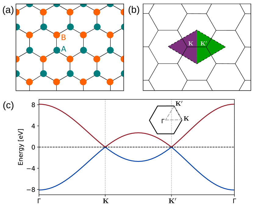
Figure 1: (a) Honeycomb lattice structure of graphene in real-space. A and B are two inequivalent carbon atoms in the unit cell. (b) The reciprocal-space lattice structure of graphene. The area within dashed lines is the reciprocal-space unit cell, whereas the areas around $\mathbf{K}$ and $\mathbf{K}^{\prime}$ valleys for integration are shaded in violet and green, respectively. (c) Energy band-structure of graphenealong high-symmetry directions in the Brillouin zone.

Time evolution of the density matrix, $\rho_{mn}^{\textbf{k}}$, is performed by solving Semiconductor Bloch equations in Houston basis as golde2008high ; mrudul2021high

$$\begin{split}\frac{\partial}{\partial t}\rho_{mn}^{\textbf{k}}=&-i\mathcal{E}_{mn}^{\textbf{k}+\textbf{A}(t)}\rho_{mn}^{\textbf{k}}-(1-\delta_{mn})\frac{\rho_{mn}^{\textbf{k}}}{T_{2}}\\ &+i\textbf{F}(t)\cdot\sum_{l}\left(\textbf{d}_{ml}^{~{}\textbf{k}+\textbf{A}(t)}\rho_{ln}^{\textbf{k}}-\textbf{d}_{ln}^{~{}\textbf{k}+\textbf{A}(t)}\rho_{ml}^{\textbf{k}}\right).\end{split}$$ (2)

Here, $\mathcal{E}^{\textbf{k}}_{mn}$ and d${}_{mn}^{\textbf{k}}$ are, respectively, energy-gaps and dipole-matrix elements between $|m,\textbf{k}\rangle$ and $|n,\textbf{k}\rangle$ states in the Brillouin zone. d${}_{mn}^{\textbf{k}}$ is defined as d${}_{mn}^{\textbf{k}}$ = -i$\left\langle u_{m}^{\textbf{k}}|\nabla_{\textbf{k}}|u_{n}^{\textbf{k}}\right\rangle$, where $u_{n}^{\textbf{k}}$ is the periodic part of the Bloch function. $\textbf{F}(t)$ and $\textbf{A}(t)$ are, respectively, the electric field and vector potential associated with the laser pulse and are related as $\textbf{F}(t)$ = -${\rm d}\textbf{A}(t)/{\rm d}t$. A phenomenological term accounting for the decoherence between electron and hole is included with a constant dephasing time $T_{2}$. The term accounting for the population relaxation, $T_{1}$, is neglected assuming $T_{1}\gg T_{2}$. The coupled differential equations in Eq. (2) are numerically solved using the fourth-order Runge-Kutta method with a time-step of 0.02 fs. The reciprocal space is sampled with a 180$\times$180 grid. The value of the dephasing time $T_{2}$ is chosen as 10 fs.

We define the valley-asymmetry parameter to quantify valley polarization as

$$\eta=\frac{n_{c}^{\mathbf{K}^{\prime}}-n_{c}^{\mathbf{K}}}{(n_{c}^{\mathbf{K}^{\prime}}+n_{c}^{\mathbf{K}})/2},$$ (3)

where $n_{c}^{\mathbf{K}}$ and $n_{c}^{\mathbf{K}^{\prime}}$ are the residual conduction band electron populations around $\mathbf{K}$ and $\mathbf{K}^{\prime}$ valleys, respectively. We estimate the total residual conduction band population, $n_{c}$, by integrating $\rho_{cc}^{\textbf{k}}$ in the reciprocal-space unit cell [see Fig. 1(b)] at the end of the laser pulse. $n_{c}^{\mathbf{K}}$ and $n_{c}^{\mathbf{K}^{\prime}}$ are obtained by integrating, respectively, within the violet and green shaded regions in Fig. 1(b), such that $n_{c}=n_{c}^{\mathbf{K}}+n_{c}^{\mathbf{K}^{\prime}}$.

The tailored laser field is a superposition of two counter-rotating circularly polarized pulses with photon energies $\omega_{1}=\omega$ and $\omega_{2}=n\omega$, respectively. This is known as $\omega-n\omega$ bi-circular field. The vector potential corresponds to this tailored field is defined as

$$\begin{split}\textbf{A}(t)=\frac{A_{0}f(t)}{\sqrt{2}}\bigg{(}&\left[\cos(\omega t+\phi)+\frac{\mathcal{R}}{n}\cos(n\omega t)\right]\hat{\textbf{e}}_{x}+\\ &\left[\sin(\omega t+\phi)-\frac{\mathcal{R}}{n}\sin(n\omega t)\right]\hat{\textbf{e}}_{y}\bigg{)}.\end{split}$$ (4)

Here, $A_{0}=F_{\omega}/\omega$ is the amplitude of the vector potential of the fundamental laser for which $F_{\omega}$ is the strength of the electric field. $f(t)$ is the temporal envelope of the driving field. The two laser fields have a sub-cycle phase difference of $\phi$ and the ratio between the two electric-field strengths is denoted by $\mathcal{R}$. In the following section, we will discuss results obtained for a seven-cycle pulse with a sin-squared envelope as used in Ref. mrudul2021light .

III Results and Discussion

Figure 2(a) presents the variation in the valley polarisation as a function of electric field strength ($F_{\omega}$) and wavelength ($\lambda$). $F_{\omega}$ and $\lambda$ are varied in the range 3-17 MV/cm and 3-6 $\mu$m, respectively. The value of the sub-cycle phase ($\phi$) is chosen as 0^∘ for which the valley polarisation is maximum. As evident from the figure, $\eta$ value corresponding to longer wavelengths and intense pulses is higher than 50%. We observe that there is no considerable valley polarisation up to a threshold value of $F_{\omega}$ and $\lambda$. Once the threshold values are reached, $\eta$ increases monotonically as a function of both $F_{\omega}$ and $\lambda$.

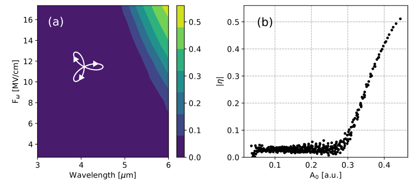
Figure 2: Dependence of the valley polarisation on the laser parameters. (a) Valley-asymmetry parameter ($\eta$) as a function of wavelength and electric field amplitude of the fundamental pulse. (b) $\eta$ as a function of the amplitude of the vector potential (A₀ = F${}_{\omega}/\omega$). Lissajous figure of the vector potential is shown in the inset of (a).

To have a better understanding, the data of Fig. 2(a) is represented as a function of $A_{0}$ of the $\omega$-field in Fig. 2(b). It is apparent that $\eta$ increases linearly with respect to $A_{0}$, after reaching the threshold value, as reflected from Fig. 2(b). This findings can be directly correlated to the mechanism of valley-polarisation in monolayer graphene as discussed in Ref. mrudul2021light . The electron dynamics in $\mathbf{K}$ and $\mathbf{K}^{\prime}$ valleys acts differently when the electrons are driven out of the isotropic part of the valleys in the reciprocal space using $\omega-2\omega$ bi-circular field. This mechanism causes different population buildup near the two valleys, resulting in considerable valley-polarisation. It is known that the dynamics of electron’s crystal momentum follows the vector potential of the electron in the reciprocal space. Therefore, the excursion length of the electron in the reciprocal space increases as the strength of the vector potential increases. It is evident that we don’t see any significant valley-polarisation up to the threshold value of the vector potential as the electron in the conduction band, generated close to the $\mathbf{K}$ points, exhibiting dynamics still in the isotropic part of the energy landscape. Once the electron reaches to the anisotropic part, the valley-polarisation scales linearly with $A_{0}$ as expected. It is important to mention that a further increase in the field strength or wavelength can result in mixing of electron population of two valleys, and the meaning of valley polarisation becomes ill-defined.

Now let us explore how the valley polarisation changes by changing the relative strength of the electric fields ($\mathcal{R}$) in $\omega-2\omega$ configuration. By varying the value of $\mathcal{R}$, Lissajous figure of the total vector potential changes substantially, while the three-fold symmetry is preserved as shown in the left panel of the Fig. 3. We present $\eta$ as a function of $\mathcal{R}$ for laser intensities of 1$\times$10¹¹W/cm² (blue, F_ω $\approx$ 9 MV/cm) and 2$\times$10¹¹W/cm² (orange, F_ω $\approx$ 12 MV/cm). As evident from the figure, the valley polarisation is maximum for $\mathcal{R}$ = 1. Moreover, there is a linear increase in the valley polarisation after $\mathcal{R}$ = 1.7 for laser intensity of 2$\times$10¹¹ W/cm².

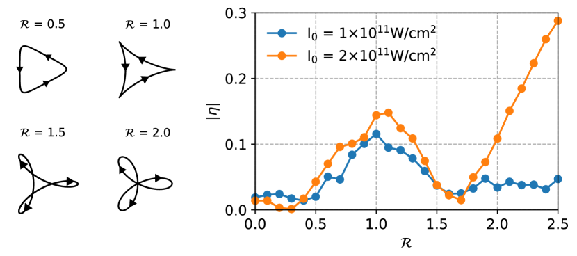
Figure 3: Effect of the ratio of the electric-field strengths, $\mathcal{R}$, on the valley polarisation. Left panel: Lissajous figures of vector potential for different ratios of the field strengths of the two pulses ($\mathcal{R}$). Right panel: Valley asymmetry parameter, $\eta$, as a function of $\mathcal{R}$ for fundamental laser intensities (I₀) of 1$\times$10¹¹ W/cm² (blue, F_ω $\approx$ 9 MV/cm ) and 2$\times$10¹¹ W/cm² (orange, F_ω $\approx$ 12 MV/cm). Here, laser pulses of 6 $\mu$m wavelength are used.

Let us recall that the contrasting dynamics of electron in two valleys is attributed to the fact that the symmetry of the vector potential matches with one of the valley, and not with the other. If this is the case then the valley polarisation will be most efficient when the total field resembles close to the energy landscape of one of the valleys for which the symmetry matches. This is what happens here, close to $\mathcal{R}$ = 1, the three-fold symmetry of the $\omega-2\omega$ fields matches closer to the energy-landscape of the conduction band, resulting in a higher valley polarisation. On the other hand, linear increase of the valley polarisation for 2$\times$10¹¹ W/cm² is due to increase of the peak of the resultant electric field with $\mathcal{R}$. The maximum field-strength scales with $\mathcal{R}$ as F_max = (1+$\mathcal{R}$)F_ω. Therefore, a linear increase in the resultant field strength for a particular value of $\mathcal{R}$ = 1.7 makes the field strong enough to push the electron out of the isotropic part.

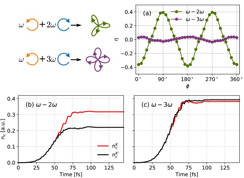
Figure 4: Valley polarisation induced by different tailored fields. (a) Valley polarisation in $\omega-2\omega$ (green) and $\omega-3\omega$ (violet) bi-circular counter-rotating fields as a function of sub-cycle phase ($\phi$). Lissajous figures corresponding to $\omega-2\omega$ and $\omega-3\omega$ fields are shown in the top left panel. Conduction band populations around $\mathbf{K}$ (red) and $\mathbf{K}^{\prime}$ (black) valleys during the laser pulse for (b) $\omega-2\omega$ and (c) $\omega-3\omega$ bi-circular counter-rotating fields.

So far we have investigated how different parameters of the $\omega-2\omega$ bi-circular field affect the valley polarisation. Let us ask an interesting question: is it only possible to achieve such a high-degree of valley polarisation using $\omega-2\omega$ bi-circular pulses or there are other configurations of tailored pulses for that purpose. To answer this question, we consider $\omega-3\omega$ bi-circular pulses and investigate what amount of valley polarisation is achievable. We use a laser intensity of 3$\times$10¹¹W/cm² and a wavelength of 6 $\mu$m. Moreover, $\mathcal{R}=2$ and $\mathcal{R}=3$ are used for $\omega-2\omega$ and $\omega-3\omega$, respectively. Lissajous figures of the total vector potentials for both the configurations are presented in Fig. 4. As evident from the figure, $\omega-2\omega$ and $\omega-3\omega$ fields have three-fold and four-fold symmetries, respectively.

The valley polarisation as a function of $\phi$ for $\omega-2\omega$ and $\omega-3\omega$ fields are presented in Fig. 4(a). As discussed earlier, $\omega-2\omega$ field generates considerable valley polarisation, and is modulated as a function of $\phi$. In contrast, $\omega-3\omega$ field generates feeble valley polarisation. We have also performed the same comparison for a laser intensity of 1$\times$10¹¹W/cm² and obtained similar observations (not shown here).

The conduction band population around $\mathbf{K}$ and $\mathbf{K}^{\prime}$ valleys during the laser pulse for $\omega-2\omega$ and $\omega-3\omega$ fields are shown in Fig. 4(b) and (c), respectively. The total conduction band population is higher in the case of $\omega-3\omega$ field, owing to the relatively higher strength of the field. In the case of $\omega-3\omega$ field, valley-polarisation fluctuates between two valleys during the laser propagation without attaining significant valley polarisation. On the other hand, a considerable, and consistent valley polarisation is visible for $\omega-2\omega$ field, once the threshold field strength is reached. In short, it is essential to use a field which breaks the inversion symmetry of the monolayer graphene to achieve a significant valley polarisation. Now let us explore an alternate way to break the inversion symmetry by using single or few-cycle pulses and analyse the valley-polarisation generated.

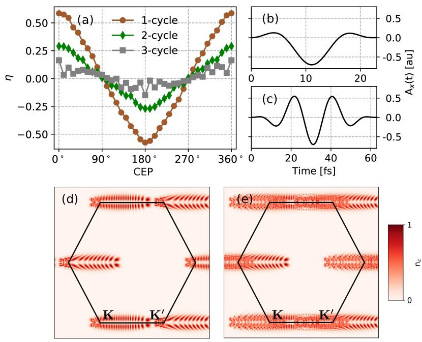
Figure 5: Valley polarisation for a single/few-cycle linearly polarised pulse. (a) $\eta$ as a function of carrier envelope phase (CEP) for a single-cycle (brown), two-cycle (green), and three-cycle linearly polarised pulses. Vector potentials for single-cycle (b) and three-cycle (c) pulses. Residual conduction band population in the first Brillouin zone induced by (d) single-cycle and (e) three-cycle pulses.

Recently, single and two-cycle circularly polarised pulses have been employed to achieve 40$\%$-60$\%$ valley polarisation in transition metal dichalcogenides. It is found that the right-handed pulse prefer to populate $\mathbf{K}$-valley, whereas left-handed pulse prefer $\mathbf{K}^{\prime}$-valley motlagh2018 . This effect is due to the topological resonance caused by laser-driven dynamics of Bloch electrons motlagh2018 . Lately, it was demonstrated that an ultrashort few-cycle linearly polarised pulse along $\Gamma-\mathbf{K}$ direction can induce significant valley polarisation in gapped-graphene materials, such as hexagonal boron nitride and transition metal dichalcogenides jimenez2021sub .

Let us revisit this mechanism of valley polarisation using short, linearly polarised pulse in gapped-graphene hexagonal materials as follows: The photon energy of the laser pulse is chosen to be much smaller than the band-gap of the material. In this case, electrons are transferred to the conduction band only close to the peak of the electric field. In contrast to relatively long linearly polarised pulses, the maximum electric field doesn’t imply zero vector potential for single or few-cycle pulses. Exploiting this fact, the electrons injected at the peak of the electric field is traversed in the momentum-space depending on the value of vector potential at that time. This mechanism results in a finite conduction band population transfer to one of the valleys of the material. The direction of electron dynamics can be controlled by changing the CEP of the pulse. This approach works only when the polarisation of the laser is along $\Gamma-\mathbf{K}$ direction as the mechanism of the valley polarisation requires the laser to have a direction connecting $\mathbf{K}$ and $\mathbf{K}^{\prime}$. As this method doesn’t depend upon the material’s Berry curvature, it applies to centrosymmetric materials. So it was anticipated that the same technique could be employed to graphene – a zero band-gap material jimenez2021sub .

Figure 5(a) present $\eta$ as a function of CEP for a single-cycle (brown), two-cycle (green), and three-cycle (grey) linearly polarised pulses along the $\Gamma-\mathbf{K}$ direction. The pulse has a peak intensity of 10¹² W/cm² and a wavelength of 6 $\mu$m. It is evident from the figure that a single-cycle pulse can induce the valley polarisation above 50$\%$. However, the valley polarisation decreases drastically as the number of cycle of the pulse increases, which can be explained as: Electrons can be injected to conduction band at any time during laser propagation. They can be traversed in conduction band as a function of the vector potential. If the laser pulse allows population dynamics preferably in +ve or -ve direction from $\mathbf{K}$-point then one of the valleys will be populated. As the pulse start becoming long by increasing the number of cycles, the preferred direction of the polarisation diminishes. As a result, the valley polarisation reduces significantly for long linearly polarised pulses as reflected from Fig. 5(a). Note that, in contrast to gapped-graphene situation, electron transfer in monolayer graphene is not limited to close to the peak of the laser pulse.

The strength of the valley polarisation modulates as a function of the pulse’s CEP as apparent from the figure. The vector potential corresponding to single-cycle, and three-cycle pulses are shown in Figs. 5(b) and (c), respectively. The variation in $\eta$ as a function of CEP can be understood as follows: The pulse is asymmetric in time for CEP = 0^∘, which translate to the transfer of electron from one valley is preferable over the other valley. As the CEP changes from 0^∘ to 180^∘, preference changes to other valley over the previous one. The vector potential becomes symmetric at CEP values of 90^∘ and 270^∘, which leads to no valley polarisation.

The residual conduction band population corresponding to the vector potentials in Figs. 5(d) and (e) are presented in Figs. 5(b) and (c), respectively. It can be observed from Fig. 5(b) that a short single-cycle pulse can push electrons towards a particular direction with respect to the $\mathbf{K}$-point, whereas three-cycle (long) pulse results in uniform distribution of conduction band population with respect to the polarisation axis. The conduction band population in Fig. 5(e) shows interference of the electronic population from two valleys since electrons are moved in both directions in this case and reduces the value of $\eta$. These interfering electrons of two valleys also result in the noisy structure of $\eta$ as reflected in Fig. 5(a).

IV Conclusions and Outlook

In summary, we have investigated few scenarios of optimising the valley polarisation in monolayer graphene using different kinds of tailored light pulses. In case of $\omega-2\omega$ bi-circular tailored pulses, the valley polarisation increases with the wavelength of the pulse. Moreover, the valley polarisation scales linearly with the strength of the vector potential. However, the value of the vector potential can’t be increased arbitrary as the electronic populations from both the valleys start overlapping and the definition of the valley polarisation becomes ill-defined. Also, intensity ratio of the $\omega-2\omega$ pulses plays an important role in the valley polarisation, and it is optimum for unit ratio. The sub-cycle phase of the $\omega-2\omega$ pulses provides another control knob, and the valley polarisation can be modulated over two valleys by tuning the sub-cycle phase. It has been found that the valley polarisation reduces drastically if one frequency in the bi-circular setup is changed from $\omega-2\omega$ to $\omega-3\omega$. Also, our findings are robust against a dephasing time of 30 fs, i.e., interband decoherence time between electron and hole.

Single and few-cycle linearly polarised pulses are also tested to induce valley polarisation. It has been observed that the single-cycle pulse can induce valley polarisation of similar strength as observed in the case of the $\omega-2\omega$ pulses. As the number of cycles in the pulse increases, valley polarisation reduces significantly. In this case, CEP provides a control knob to modulate the valley polarisation from one valley to other. The underlying mechanisms of valley polarisation in $\omega-2\omega$ bi-circular and single or few-cycle linearly polarised pulses are entirely different. However, while fixing the laser parameters for a particular method, one needs to take the damage threshold of graphene into considereation roberts2011response . Furthermore, high-harmonic spectroscopy would be an appropriate appraoch to read the valley polarisation induced by both the methods jimenez2021sub ; mrudul2021light .

We think that controlling the sub-cycle phase between $\omega-2\omega$ bi-circular long pulses is “relatively easy” in comparison to the generation and control of a single-cycle pulse. Moreover, one could imagine of employing half-cycle or fraction of single-cycle pulse to improve the valley contrast, but it will be a daunting task experimentally. It will be interesting to see the realisation of different logical operations and device fabrications using the valley polarisation in monolayer graphene as it has been done in similar materials jana2021robust ; sin2017valleytronics . Moreover, the bandgap at $\mathbf{K}$ and $\mathbf{K}^{\prime}$ remain zero as we move monolayer to bilayer graphene. Also, the energy contour in bilayer graphene exhibits trigonal structures around $\mathbf{K}$ and $\mathbf{K}^{\prime}$ valleys. Therefore, we believe that our findings remain valid for bilayer graphene qualitatively.

References

- (1) Novoselov, K. S. et al. Two-dimensional atomic crystals. Proceedings of the National Academy of Sciences 102, 10451–10453 (2005).
- (2) Neto, A. H. C., Guinea, F., Peres, N. M. R., Novoselov, K. S. & Geim, A. K. The electronic properties of graphene. Reviews of Modern Physics 81, 109 (2009).
- (3) Geim, A. K. Graphene: status and prospects. Science 324, 1530–1534 (2009).
- (4) Vitale, S. A. et al. Valleytronics: opportunities, challenges, and paths forward. Small 14, 1801483 (2018).
- (5) Schaibley, J. R. et al. Valleytronics in 2d materials. Nature Reviews Materials 1, 16055 (2016).
- (6) Gorbachev, R. V. et al. Detecting topological currents in graphene superlattices. Science 346, 448–451 (2014).
- (7) Yankowitz, M. et al. Emergence of superlattice dirac points in graphene on hexagonal boron nitride. Nature Physics 8, 382–386 (2012).
- (8) Hunt, B. et al. Massive dirac fermions and hofstadter butterfly in a van der waals heterostructure. Science 340, 1427–1430 (2013).
- (9) Rycerz, A., Tworzydło, J. & Beenakker, C. W. J. Valley filter and valley valve in graphene. Nature Physics 3, 172–175 (2007).
- (10) Grujić, M. M., Tadić, M. Ž. & Peeters, F. M. Spin-valley filtering in strained graphene structures with artificially induced carrier mass and spin-orbit coupling. Physical Review Letters 113, 046601 (2014).
- (11) Settnes, M., Power, S. R., Brandbyge, M. & Jauho, A. P. Graphene nanobubbles as valley filters and beam splitters. Physical Review Letters 117, 276801 (2016).
- (12) Faria, D., León, C., Lima, L. R. F., Latgé, A. & Sandler, N. Valley polarization braiding in strained graphene. Physical Review B 101, 081410 (2020).
- (13) Xiao, D., Yao, W. & Niu, Q. Valley-contrasting physics in graphene: magnetic moment and topological transport. Physical Review Letters 99, 236809 (2007).
- (14) Mak, K. F., He, K., Shan, J. & Heinz, T. F. Control of valley polarization in monolayer mos2 by optical helicity. Nature Nanotechnology 7, 494–498 (2012).
- (15) Jones, A. M. et al. Optical generation of excitonic valley coherence in monolayer wse2. Nature Nanotechnology 8, 634–638 (2013).
- (16) Gunlycke, D. & White, C. T. Graphene valley filter using a line defect. Physical Review Letters 106, 136806 (2011).
- (17) Xiao, D., Liu, G. B., Feng, W., Xu, X. & Yao, W. Coupled spin and valley physics in monolayers of mos 2 and other group-vi dichalcogenides. Physical Review Letters 108, 196802 (2012).
- (18) Langer, F. et al. Lightwave valleytronics in a monolayer of tungsten diselenide. Nature 557, 76 (2018).
- (19) Jiménez-Galán, Á., Silva, R. E. F., Smirnova, O. & Ivanov, M. Lightwave topology for strong-field valleytronics. arXiv arXiv–1910 (2019).
- (20) Jiménez-Galán, Á., Silva, R. E., Smirnova, O. & Ivanov, M. Sub-cycle valleytronics: control of valley polarization using few-cycle linearly polarized pulses. Optica 8, 277–280 (2021).
- (21) Mrudul, M., Jiménez-Galán, Á., Ivanov, M. & Dixit, G. Light-induced valleytronics in pristine graphene. Optica 8, 422–427 (2021).
- (22) Mrudul, M. S., Tancogne-Dejean, N., Rubio, A. & Dixit, G. High-harmonic generation from spin-polarised defects in solids. npj Computational Materials 6, 1–9 (2020).
- (23) Mrudul, M. S., Pattanayak, A., Ivanov, M. & Dixit, G. Direct numerical observation of real-space recollision in high-order harmonic generation from solids. Physical Review A 100, 043420 (2019).
- (24) Neufeld, O., Tancogne-Dejean, N., De Giovannini, U., Hübener, H. & Rubio, A. Light-driven extremely nonlinear bulk photogalvanic currents. Physical Review Letters 127, 126601 (2021).
- (25) Pattanayak, A., Mrudul, M. S. & Dixit, G. Influence of vacancy defects in solid high-order harmonic generation. Physical Review A 101, 013404 (2020).
- (26) Ansari, I. N. et al. Controlling polarization of attosecond pulses with plasmonic-enhanced bichromatic counter-rotating circularly polarized fields. Physical Review A 103, 013104 (2021).
- (27) Dixit, G., Jiménez-Galán, Á., Medišauskas, L. & Ivanov, M. Control of the helicity of high-order harmonic radiation using bichromatic circularly polarized laser fields. Physical Review A 98, 053402 (2018).
- (28) Heinrich, T. et al. Chiral high-harmonic generation and spectroscopy on solid surfaces using polarization-tailored strong fields. Nature Communications 12, 1–7 (2021).
- (29) Heide, C., Boolakee, T., Higuchi, T. & Hommelhoff, P. Sub-cycle temporal evolution of light-induced electron dynamics in hexagonal 2d materials. Journal of Physics: Photonics 2, 024004 (2020).
- (30) Kelardeh, H. K., Apalkov, V. & Stockman, M. I. Attosecond strong-field interferometry in graphene: Chirality, singularity, and berry phase. Physical Review B 93, 155434 (2016).
- (31) Heide, C., Higuchi, T., Weber, H. B. & Hommelhoff, P. Coherent electron trajectory control in graphene. Physical Review Letters 121, 207401 (2018).
- (32) Higuchi, T., Heide, C., Ullmann, K., Weber, H. B. & Hommelhoff, P. Light-field-driven currents in graphene. Nature 550, 224 (2017).
- (33) Kundu, A., Fertig, H. & Seradjeh, B. Floquet-engineered valleytronics in dirac systems. Physical Review Letters 116, 016802 (2016).
- (34) Friedlan, A. & Dignam, M. M. Valley polarization in biased bilayer graphene using circularly polarized light. Physical Review B 103, 075414 (2021).
- (35) Reich, S., Maultzsch, J., Thomsen, C. & Ordejon, P. Tight-binding description of graphene. Physical Review B 66, 035412 (2002).
- (36) Trambly de Laissardière, G., Mayou, D. & Magaud, L. Localization of dirac electrons in rotated graphene bilayers. Nano letters 10, 804–808 (2010).
- (37) Moon, P. & Koshino, M. Energy spectrum and quantum hall effect in twisted bilayer graphene. Physical Review B 85, 195458 (2012).
- (38) Golde, D., Meier, T. & Koch, S. W. High harmonics generated in semiconductor nanostructures by the coupled dynamics of optical inter-and intraband excitations. Physical Review B 77, 075330 (2008).
- (39) Mrudul, M. & Dixit, G. High-harmonic generation from monolayer and bilayer graphene. Physical Review B 103, 094308 (2021).
- (40) Motlagh, S. A. O., Wu, J. -S., Apalkov, V., & Stockman, M. I. Femtosecond valley polarization and topological resonances in transition metal dichalcogenides. Physical Review B 98, 081406 (2018).
- (41) Roberts, A. et al. Response of graphene to femtosecond high-intensity laser irradiation. Applied Physics Letters 99, 051912 (2011).
- (42) Jana, K. & Muralidharan, B. Robust all-electrical topological valley filtering using monolayer 2d-xenes. arXiv preprint arXiv:2107.13318 (2021).
- (43) Ang, Y. S., Yang, S. A., Zhang, C., Ma, Z. & Ang, L. K. Valleytronics in merging dirac cones: All-electric-controlled valley filter, valve, and universal reversible logic gate. Phys. Rev. B 96, 245410 (2017).