Linear algebra with transformers

Abstract

Transformers can learn to perform numerical computations from examples only. I study nine problems of linear algebra, from basic matrix operations to eigenvalue decomposition and inversion, and introduce and discuss four encoding schemes to represent real numbers. On all problems, transformers trained on sets of random matrices achieve high accuracies (over $90\%$). The models are robust to noise, and can generalize out of their training distribution. In particular, models trained to predict Laplace-distributed eigenvalues generalize to different classes of matrices: Wigner matrices or matrices with positive eigenvalues. The reverse is not true.

1 Introduction

Since their introduction for machine translation by Vaswani et al. (2017), transformers were applied to a wide range of problems, from text generation (Radford et al., 2018; 2019) to image processing (Carion et al., 2020) and speech recognition (Dong et al., 2018), where they now achieve state-of-the-art performance (Dosovitskiy et al., 2021; Wang et al., 2020b). Transformers have also been proposed for problems of symbolic mathematics, like integration (Lample & Charton, 2019), theorem proving (Polu & Sutskever, 2020), formal logic (Hahn et al., 2021), SAT solving (Shi et al., 2021), symbolic regression (Biggio et al., 2021) and dynamical systems Charton et al. (2020). In these works, transformers perform symbolic computations, i.e. manipulate abstract mathematical symbols.

Beyond symbol manipulation, mathematics also involve numerical calculations (e.g. arithmetic, numerical solutions of equations). On these tasks, experiments with transformers and other sequence models have been disappointing. Basic arithmetic operations, like multiplication or modulus, prove very difficult to learn (Kaiser & Sutskever, 2015; Palamas, 2017), and models struggle with generalization out of their training distribution (Nogueira et al., 2021). It could even be shown (Shalev-Shwartz et al., 2017) that some arithmetic tasks cannot be solved using gradient descent. Such results might severely restrict the applicability of transformers in science. Most practical problems of mathematics mix symbolic and numerical computations. If transformers “cannot compute”, their use in science is very limited.

In this paper, I investigate the capability of transformers to learn to perform numerical computations with high accuracy. I focus on nine problems of linear algebra, from basic operations on dense matrices to inversion, eigen and singular value decomposition. I show that small transformers can be trained, from examples only, to compute approximate solutions (up to a few percents of the $L^{1}$ norm) with more than $90\%$ accuracy (over $99\%$ in most cases). I propose and discuss four encodings to represent real numbers, and train small sequence to sequence transformers (up to 6 layers, 10 to 50 million trainable parameters) from generated datasets of random matrices. I investigate different architectures, in particular asymmetric configurations where the encoder or decoder has only one layer. Finally, I show that the models are robust to noisy data, and that they can generalize out of their training distribution if special attention is paid to training data generation.

Caveat. This paper does not advocate replacing existing linear algebra algorithms with transformer-based implementations. Numerical packages are faster, more accurate, and scale better. My motivation is twofold: better understand the capabilities and limitations of transformers in mathematics, and investigate their potential use as tools for the emerging field of AI for science.

In applications to mathematics, while previous research has shown that transformers struggle with basic arithmetic, I demonstrate that they can learn complex computations, like eigenvalue decomposition. I also show that leveraging the theory of random matrices can help understand the mechanisms of out-of-domain generalization, a known limitation of transformers in mathematics (Welleck et al., 2021), and a difficult problem because of the lack of metrics over problem space.

Beyond mathematics, transformers are fast becoming the “default model” for many deep learning applications. Their potential use as end to end tools for AI for Science has received a lot of attention recently. I believe that demonstrating that transformers can handle some of the computational building blocks of many scientific problems, like the problems of linear algebra discussed here, is a pre-requisite to their wider generalization.

The source code for the model and experiments is available at github.com/facebookresearch/LAWT.

2 Problems and datasets

Let $M$ and $N$ be $m\times n$ real matrices and $V\in\mathbb{R}^{m}$ . This paper considers nine problems of linear algebra:

• matrix transposition: find $M^{T}$, a $n\times m$ matrix,

• matrix addition: find $M+N$, a $m\times n$ matrix,

• matrix-vector multiplication: find $M^{T}V$, in $\mathbb{R}^{n}$,

• matrix multiplication: find $M^{T}N$, a $n\times n$ matrix,

• eigenvalues: $M$ symmetric, find its $n$ (real) eigenvalues, sorted in descending order,

• eigenvectors: $M$ symmetric, find $D$ diagonal and $Q$ orthogonal such that $QMQ^{T}=D$, set as a $(n+1)\times n$ matrix, with (sorted) eigenvalues in its first row,

• singular values: find the $n$ eigenvalues of $M^{T}M$, sorted in descending order,

• singular value decomposition: find orthogonal $U,V$ and diagonal $S$ such that $S=UMV$, set as a $(m+n+1)\times min(m,n)$ matrix,

• inversion: $M$ square and invertible, find its inverse $P$, such that $MP=PM=Id$.

These problems range from operations on single coefficients of the matrices (transposition and addition), to computations over rows and columns, involving several arithmetic operations (multiplication), and complex nonlinear transformations involving the whole matrix (decompositions and inversion).

For each problem, the training data is generated by sampling random input matrices $I$ (see section 2.2), and computing the output $O$ with a linear algebra package (NumPy linalg). All coefficients in $I$ and $O$ are set in base ten floating-point representation, and rounded to three significant digits in the mantissa. If a problem has several input or output matrices, they are concatenated into one (for instance, the two $m\times n$ operands of the addition task are concatenated into one $m\times 2n$ matrix $I$).

2.1 Encoding matrices as sequences

The input and output to all problems studied here are matrices. Transformers process sequences of tokens. To encode a $m\times n$ matrix as a sequence, its dimensions are encoded as two symbolic tokens (Vm and Vn), and its $mn$ coefficients are then enumerated and encoded. I propose four encoding schemes for matrix coefficients (set in scientific notation with three significant digits): P10, P1000, B1999, and FP15.

Base 10 positional encoding (P10) represents numbers as sequences of five tokens : one sign token (+ or -), $3$ digits (from 0 to 9) for the mantissa, and a symbolic token (from E-100 to E+100) for the exponent. For instance, $3.14$ is represented as $314.10^{-2}$, and encoded as [+, 3, 1, 4, E-2].

Base 1000 positional encoding (P1000) provides a more compact representation. The mantissa is encoded as a single token (from 0 to 999) and a number is represented as the triplet (sign, mantissa, exponent).

Balanced base 1999 (B1999) encodes the sign and mantissa as a single token (from -999 to 999).

15 bit floating point (FP15) encodes a floating point number $x=m10^{b}$ as a single token FPm/b.

Table 1 provides examples for the four encodings. More information can be found in Appendix A.

Encoding	$3.14$	$-6.02.10^{23}$	Tokens / coefficient	Size of vocabulary
P10	[+, 3, 1, 4, E-2]	[-, 6, 0, 2, E21]	5	210
P1000	[+, 314, E-2]	[-, 602, E21]	3	1100
B1999	[314, E-2]	[-602, E21]	2	2000
FP15	[FP314/-2]	[FP-602/21]	1	30000

Table 1: Four encodings for matrix coefficients.

Choosing an encoding is a trade-off. Long encodings (P10, P1000) use a small vocabulary, and embed knowledge about numbers that the model can use (e.g. that numbers can be crudely compared from their signs and exponents only, that addition and multiplication can be learned by memorizing small tables). Compact encodings use a larger vocabulary (harder to learn) but result in shorter sequences that facilitate training with transformers. In P10, a $20\times 20$ matrix is a sequence of $2002$ tokens, close to the practical limit of transformers with quadratic attention. In FP15, it is only $402$ tokens long.

The decision to round matrix coefficients to three significant digits is mainly motivated by the need to keep FP15 vocabulary at sizes that small transformers can learn without pre-training. Experiments about the impact of number precision can be found in appendix C.

2.2 Random matrix generation

In most experiments, training and test data are random matrices with coefficients uniformly distributed in $[-A,A]$ (with $A=10$). When symmetric, these matrices are known as Wigner matrices. Their eigenvalues have a centered distribution with standard deviation $\sigma=A\sqrt{n/3}$ (see Mehta (2004) and Appendix H) that converges as $n$ grows to the semi-circle law $p(\lambda)=\sqrt{4\sigma^{2}-\lambda^{2}}/{(2\pi\sigma^{2})}$. If the coefficients follow a gaussian distribution, the associated eigenvectors are uniformly distributed over the unit sphere.

In section 4.4, while investigating out-of-distribution generalization, I will need to generate random symmetric matrices with specific eigenvalue distributions (i.e. classes of random matrices with non-independent coefficients). To this effect, I sample random symmetric matrices $M$ with gaussian coefficients, and compute their eigenvalue decomposition $M=PDP^{T}$, with $P$ an orthogonal matrix of eigenvectors (uniformly distributed over the unit sphere because the coefficients are gaussian). Replacing $D$, the diagonal matrix of eigenvalues of $M$, with a diagonal $D^{\prime}$ sampled from a different distribution, and recomputing $M^{\prime}=PD^{\prime}P^{T}$, yields a symmetric matrix (since $P$ is orthogonal) with eigenvalues following the desired distribution, and eigenvectors uniformly distributed over the unit sphere.

3 Models and experimental settings

Models and training. All models use the transformer architecture from Vaswani et al. (2017): an encoder and a decoder connected by cross-attention. Models have $512$ dimensions, $8$ attention heads and up to $6$ layers (experiments with larger models can be found in Appendix D.3). Training is supervised, minimizes the cross-entropy between model predictions and correct solutions, and uses the Adam optimiser (Kingma & Ba, 2014) with a learning rate of $10^{-4}$, a linear warm-up phase of 10,000 steps and cosine scheduling (Loshchilov & Hutter, 2016). Training data is generated on the fly in batches of $64$. All models are trained on an internal cluster, using NVIDIA Volta GPU with 32GB memory. Basic operations on matrices and eigenvalues train on 1 GPU in less than a day (from a few hours for transposition and addition, to a day for multiplication and eigenvalues). Eigenvectors, SVD and inversion train on 4 GPU, and take from 3 days to a week.

Evaluation. At the end of every epoch (300,000 examples), a random test set (10,000 examples) is generated and model accuracy is evaluated. A predicted sequence is a correct solution to the problem $(I,O)$ ($I$ and $O$ the input and output matrices) if it can be decoded as a valid matrix $P$ and approximates the correct solution to a given tolerance $\tau$. In most problems, I check that $P$ verifies $\|P-O\|<\tau\|O\|$. When computing eigenvectors, I verify that the predicted solution $(Q,D)$ can reconstruct the input matrix, $\|QIQ^{T}-D\|<\tau\|D\|$. For singular value decomposition, I check that $\|UIV-S\|<\tau\|S\|$, and for matrix inversion, that $\|PI-Id\|<\tau\|Id\|=\tau$. The $L^{1}$ norm, $\|A\|=\sum_{i,j}{|a_{i,j}|}$, for $A=(a_{i,j})$, is used in all experiments. With other norms, like $L^{2}$ or $L^{\infty}$, the error is weighted in favor of correct predictions of the largest coefficients in the solution. For eigenvalue and singular value prediction, this amounts to finding the largest values, a different and easier problem. More discussion and comparisons between norms can be found in Appendix B.

Numerical tolerance. All results are provided with tolerance $\tau$ between $0.5$ and $5\%$. Since coefficients are rounded to three significant digits, $0.5\%$ is the best we can achieve when computations are subject to rounding error. As computations become more complex, error accumulates, and larger values of $\tau$ should be considered. I consider $\tau=0\%$ for transposition, $\tau=1\%$ for basic matrix operations (addition and multiplication), and $\tau=2$ or $5\%$ for non linear operations (decomposition, inversion).

Problem size. All experiments are performed on dense matrices. In most cases, I focus on $5\times 5$ matrices (or rectangular matrices with as many coefficients: e.g. $6\times 4,2\times 13$), and scale to larger dimensions, from $8\times 8$ to $15\times 15$, and datasets of matrices with variable dimensions (e.g. $5\times 5$ to $15\times 15$). In this paper, the emphasis is on problems that can be solved by small transformers (up to 6 layers). I discuss scaling and larger models in Appendix D.3.

4 Experiments and results

This section presents experimental results for the nine problems considered. I compare encodings for different matrix sizes and tolerance levels, using the best choice of hyperparameters for each problem (i.e. the smallest architecture that can achieve high accuracy). I also show that our models are robust to noise in the training data. Learning curves and experiments with model size can be found in Appendix D, alternative architectures in Appendix E.1 (LSTM and GRU) and E.2 (universal transformers), and additional tasks (re-training, joint training) in Appendix F.

4.1 Transposition

Learning to transpose a matrix amounts to learning a permutation of its elements. For a square matrix, all cycles in the permutation have length $1$ or $2$. Longer cycles may appear in rectangular matrices. This task involves no arithmetic operations: tokens in the input sequence are merely copied to different positions in the output. This paper investigates two cases. In the fixed-dimension case, all matrices in the dataset have the same dimensions and only one permutation must be learned. In the variable-dimension case, the dataset includes matrices of different formats, and several permutations must be learned (one per matrix format). In these experiments, models have one layer, $256$ dimensions and $8$ attention heads, and use the four encodings.

After training, all models achieve $99\%$ exact accuracy ($0\%$ tolerance) for fixed-size matrices with dimensions up to $30\times 30$. This holds for all encodings and input and output sequence lengths up to $2000$ tokens. The variable-size case proves more difficult, because the model must learn many different permutations. Still, the model achieve $99\%$ accuracy on matrices with $5$ to $15$ dimensions, and $96\%$ for matrices with $5$ to $20$ dimensions. Table 2 summarizes the results.

	Fixed dimensions							Variable dimensions
								Square		Rectangular
	5x5	10x10	20x20	30x30	5x6	7x8	9x11	5-15	5-20	5-15	5-20
P10	100	100	100	-	100	100	100	100	-	97.0	-
P1000	100	100	99.9	-	100	100	100	99.9	-	98.4	-
B1999	100	100	99.9	100	100	100	100	100	96.6	99.6	91.4
FP15	99.8	99.5	99.4	99.8	99.8	99.5	99.3	99.8	99.6	99.4	96.1

Table 2: Exact prediction of matrix transposition for different matrix dimensions. Transformers with one layer, 256 dimensions and 8 attention heads.

4.2 Addition

To add two $m\times n$ matrices, the model must learn the correspondence between input and output positions and the algorithm for adding two numbers in scientific notation. Then, it must apply the algorithm to $mn$ pairs of coefficients. In these experiments, models have one or two layers, $8$ attention heads and $512$ dimensions.

All models achieve $99\%$ accuracy at $1\%$ tolerance ($98\%$ at $0.5\%$) on sums of fixed-size matrices with dimensions up to $10\times 10$, for all four encodings. B1999 models achieve $99.5\%$ accuracy at $0.5\%$ tolerance for $15\times 15$ matrices and $87.9\%$ accuracy at $1\%$ tolerance on $20\times 20$ matrices. As dimensions increase, models using long encodings (P1000 and P10) become more difficult to train as their input sequences grow longer. For instance, adding two $15\times 15$ matrices involves $450$ coefficients, an input of $1352$ tokens in P1000 and $2252$ in P10.

On variable-size matrices, models achieve $99.5\%$ accuracy at $1\%$ tolerance for dimensions up to $10$, with 2-layer transformers using the B1999 encoding. Their accuracy drops to $48$ and $37\%$ for square and rectangular matrices with $5$ to $15$ dimensions. This can be mitigated by increasing the depth of the decoder: models with one layer in the encoder and $6$ in the decoder achieve $77$ and $87\%$ accuracy. Table 3 summarizes these results.

	Fixed dimensions						Variable dimensions
							Square			Rectangular
Size	5x5	6x4	3x8	10x10	15x15	20x20	5-10	5-15	5-15	5-10	5-15	5-15
Layers	2/2	2/2	2/2	2/2	2/2	1/1	2/2	1/1	1/6	2/2	2/2	1/6
$5\%$	100	99.9	99.9	100	100	98.8	100	63.1	99.3	100	72.4	99.4
$2\%$	100	99.5	99.8	100	100	98.4	99.8	53.3	88.1	99.8	50.8	94.9
$1\%$	100	99.3	99.7	100	99.9	87.9	99.5	47.9	77.2	99.6	36.9	86.8
$0.5\%$	100	98.1	98.9	100	99.5	48.8	98.9	42.6	72.7	99.1	29.7	80.1

Table 3: Accuracies of matrix sums, for different tolerances. B1999 encoding, 512 dimension and 8 attention heads.

4.3 Multiplication

Multiplication of a matrix $M$ of dimension $m\times n$ by a vector $V\in\mathbb{R}^{n}$ amounts to computing $m$ dot products between $V$ and the lines of $M$. Each calculation features $n$ multiplications and $n-1$ additions, and involves one row in the matrix and all coefficients in the vector. The model must now learn two operations: add and multiply. Experiments with models with $1$ and $2$ layers show that high accuracy can only be achieved with the P10 or P1000 encoding, with P1000 performing better on average. The number of layers, on the other hand, makes little difference.

	P10	P1000			P1000				Variable 5-10 (P1000)
	5x5	5x5	10x10		14x2	9x3	4x6	2x10	Square	Rectangular
Tolerance	2/2 layers	2/2	2/2		1/1	1/1	2/2	2/2	4/4	2/2
$5\%$	100	100	100		99.3	99.9	100	100	72.4	41.7
$2\%$	99.9	100	100		99.0	99.7	100	99.8	68.4	35.0
$1\%$	98.5	99.9	99.9		98.7	99.5	99.9	99.2	60.1	20.1
$0.5\%$	81.6	99.5	98.4		98.1	99.0	98.6	94.5	30.8	4.4

Table 4: Accuracies of matrix-vector products, for different tolerances. All model have 512 dimensions and 8 heads.

	Square matrices			Rectangular matrices
	5x5	5x5		2x13	2x12	3x8	4x6	6x4	8x3	12x2	13x2
Tolerance	P10 2/2 layers	1/4		4/4	4/4	2/6	1/4	1/6	1/6	1/6	1/4
$5\%$	100	100		100	100	100	100	100	100	100	99.9
$2\%$	100	100		100	100	100	100	100	100	99.7	99.8
$1\%$	99.8	100		99.9	100	100	99.9	100	99.9	99.3	99.8
$0.5\%$	64.5	99.9		97.1	98.5	99.6	99.7	99.5	99.5	99.0	99.8

Table 5: Accuracy of matrix multiplication, for different tolerances. Fixed-size matrices with 24-26 coefficients. All encodings are P1000 unless specified. Models have 512 dimensions and 8 attention heads.

On this task, models achieve $99.9\%$ accuracy at $1\%$ tolerance for $5\times 5$ and $10\times 10$ square matrices, and $99\%$ for rectangular matrices with about $30$ coefficients. The variable-size case proves much harder. Models achieve non-trivial results: $60\%$ accuracy with $1\%$ tolerance for square matrices, but larger models are needed for high accuracy. Table 4 summarizes the results.

Multiplication of matrices $M$ and $P$ is a scaled-up version of matrix-vector multiplication, now performed for every column in matrix $P$. As above, high accuracy is only achieved with the P10 and P1000 encoding. Models achieve $99\%$ accuracy at $1\%$ tolerance for $5\times 5$ square matrices and rectangular matrices of comparable dimensions (see Table 5). Performance is the same as matrix-vector multiplication, a simpler task. However, matrix multiplication needs deeper models (especially decoders), and more training time.

4.4 Eigenvalues

Compared to basic operations on matrices, computing the eigenvalues of symmetric matrices is a much harder problem, non-linear and typically solved by iterative algorithms. Deeper models, with $4$ or $6$ layers, are used in this task. They achieve $100\%$ accuracy at $5\%$ tolerance, and $99\%$ at $2\%$, for $5\times 5$ and $8\times 8$ matrices. High accuracy is achieved with all four encodings, but P1000 proves more efficient with $8\times 8$ matrices.

On fixed-size datasets, scaling to larger problems proves difficult. It takes 360 million examples for our best models to reach $25\%$ accuracy on $10\times 10$ matrices. As a comparison, 40 million examples are required to train $5\times 5$ models to $99\%$ accuracy, and 60 million for 8$\times$8 models. This limitation can be overcome by training on variable-size datasets, achieving $100\%$ accuracy at $5\%$ tolerance, and $100,100$ and $76\%$ at $2\%$, for sets of 5-10, 5-15 and 5-20 matrices. Table 6 summarizes the results.

	Fixed dimensions							Variable dimensions
	5x5	5x5	5x5	5x5	8x8	8x8	10x10	5-10	5-15	5-20
Encoding	P10	P1000	B1999	FP15	P1000	FP15	FP15	FP15	FP15	FP15
Layers	6/6	4/1	6/6	6/1	6/1	1/6	1/6	4/4	6/6	4/4
$5\%$	100	100	100	100	100	100	25.3	100	100	100
$2\%$	100	99.9	100	100	99.2	97.7	0.4	99.8	100	75.5
$1\%$	99.8	98.5	98.6	99.7	84.7	77.9	0	87.5	94.3	45.3
$0.5\%$	93.7	88.5	73.0	91.8	31.1	23.9	0	37.2	40.6	22.5

Table 6: Accuracy of eigenvalues for different tolerances and dimensions. All models have 512 dimensions and 8 attention heads, except the 10x10 model, which has 510 and 12.

Larger models.

In the fixed-dimension case, 6-layer models are limited to $8\times 8$ matrices. Experiments with deeper models show that they can solve larger problems. For instance, 12-layer transformers can compute the eigenvalues of $12\times 12$ matrices. Large models also need less examples to train to high accuracy. Table 7 summarizes these results. Detailed results are in Appendix D.3

	Accuracy			Sample size (millions)
Layers	1/8	1/12	1/24	1/8	1/12	1/24
$8\times 8$ matrices	100	100	100	28.8	11.4	11.1
$10\times 10$ matrices	100	100	100	85.2	36.6	32.1
$12\times 12$ matrices	3	97	100	-	-	99.3

Table 7: Eigenvalues, larger models. Accuracy to 5% tolerance, and sample size to reach 99% accuracy.

4.5 Eigenvectors

In this task, the model predicts both the eigenvalues and an associated orthogonal matrix of eigenvectors. Models using the P10 and P1000 encoding achieve $97$ and $94\%$ accuracy at $5\%$ tolerance for $5\times 5$ matrices. P1000 models also reach $82\%$ accuracy on $6\times 6$ matrices. Whereas FP15 models only reach $52\%$ accuracy, an asymmetric model, coupling a 6-layer FP15 encoder and a 1-layer P1000 decoder, achieves $94\%$ accuracy at $5\%$ and $87$ at $2\%$, the best result on this task. Table 8 summarizes these results.

	5x5					6x6
	P10	P1000	FP15	FP15/P1000		P1000
	4/4 layers	6/6	1/6	6/1		6/1
$5\%$	97.0	94.0	51.6	93.5		81.5
$2\%$	83.4	77.9	12.6	87.4		67.2
$1\%$	31.2	41.5	0.6	67.5		11.0
$0.5\%$	0.6	2.9	0	11.8		0.1

Table 8: Accuracies of eigenvectors, for different tolerances and depths (512 dimensions, 8 heads).

Analysis of failure cases.

On this task, models achieve significantly less than $100\%$ accuracy. This makes it possible to investigate failure cases. For this analysis, I use the trained FP15/P1000 6/1 layer model from table 8 ($93\%$ accuracy), generate a new test sample of 10 000 problems, predict solutions, and evaluate performance on various metrics. On this new test set, the model achieves $91.1\%$ accuracy with $5\%$ tolerance, and $82.1$, $45.2$ and $1.4\%$ at $2$, $1$ and $0.5$ tolerance.

First, one notes that almost all model predictions (9999 out of 10000) are well-formed matrices: the model produces no meaningless output, such as incorrect encoding of numbers, or matrices with the wrong number of elements. This is consistently observed in all experiments: output syntax is learned to near-perfection at the beginning of training. Also, accuracy increases with tolerance: $95.6\%$ accuracy at $25\%$ tolerance. This suggests that, even when they fail to predict the correct solution, models do not hallucinate irrelevant predictions (as was reported on natural language tasks). Instead, they predict syntactically correct solutions that often turn out to be “rough approximations” of the correct answer.

When computing eigenvectors, the model predicts two matrices, a diagonal matrix of eigenvalues $D$ and an orthogonal matrix of eigenvectors $H$. Accuracy is measured as the $L^{1}$ distance between $H^{T}IH$ ($I$ the input matrix) and $D$, i.e. how well $H$ diagonalizes the input into $D$. A different metric, the distance between $HDH^{T}$ and $I$, could be used instead, which is associated to a related, but weaker, problem: finding approximations to $I$ of the form $HDH^{T}$ ($D$ diagonal). With this metric, the model achieves slightly higher accuracy: $95.7\%$ at $5\%$ tolerance ($92.9$, $88.4$ and $73.0$ at $2$, $1$ and $0.5\%$). This confirms our previous observation that, in many failure cases, the model predicts solutions that are “somehow relevant” to eigen decomposition (here, solutions to the weak problem).

We also know from theory that $D$ should contain the eigenvalues of the input matrices, and that $H$ should be orthogonal (all lines and columns orthogonal, with unit norm). Translating these properties into metrics can help us understand failure cases, and the relevance of incorrect model predictions.

First, eigenvalues are always correctly predicted: the corresponding accuracy is $100\%$ at $5\%$ tolerance, and $99.4\%$ at $0.5\%$. The (easier) sub-task of eigenvalue prediction has been learned by the model. Second, all the norms of the columns of $H$ are within $5\%$ of $1$ in $99.9\%$ of the test examples (within $1\%$ in $99.2\%$). All predicted eigenvectors have unit norm. This indicates that failed model predictions actually succeed in computing the eigenvalues, and a set of unit vectors. In other words, those two properties of eigen decomposition have been learned by the model, in the sense that they are respected even in incorrect predictions.

To measure the orthogonality of the eigenvectors, I compute the dot products of successive eigenvectors, which should be all be $0$. On the test set, all dot products are within $-0.05$ and $0.05$ in $93.6$ of the cases (and within $-0.01$ and $0.01$ in $85.1$). This suggests that when the model fails, it proveds the correct eigenvalues, and unit eigenvectors, but fails to make the “eigenvectors” strictly orthogonal. This observation suggests a criterion for predicting model accuracy: we can test the orthogonality of predicted $H$ by measuring its condition number (the ratio of its largest and smallest singular values), which should be one if $H$ is orthogonal, and larger if it is not. In fact, in $98\%$ of correct predictions, the predicted $H$ has a condition number smaller than $1.035$. For $98\%$ of failures, the condition number of $H$ is larger than $1.04$.

To summarize, when trained on eigen decomposition, the model learns the easier sub-task of predicting eigenvalues, with $100\%$ accuracy. It also learns to preserve theoretical properties of the result, like the unit norm of eigenvectors, and their (approximate) orthogonality. All failures concentrate on one specific sub-task: orthogonalizing the eigenvectors. This allows us to derive an accurate predictor of model failure: the condition number of the predicted matrix $H$.

4.6 Inversion

Computing the inverses of 5$\times$5 matrices proves the hardest task so far. Models using the P10 and P1000 encodings, with 6-layer encoders and 1-layer decoders and $8$ attention heads, achieve $74$ and $80\%$ accuracy at $5\%$ tolerance. Adding more heads in the encoder bring no gain in accuracy, but makes training faster: $8$-head models need 250 millions examples to train to $75\%$ accuracy, $10$ and $12$-head models only $120$. As in the previous task, asymmetric models achieve the best results. $90\%$ accuracy at $5\%$ tolerance can be reached with a 6-layer FP15 encoder with $12$ attention heads, and a 1-layer P1000 decoder with $8$ heads.

	P10	P1000				FP15/P1000
Tolerance	8/8 heads	8/8 heads	10/8 heads	12/8 heads		10/4 heads	12/8 heads
$5\%$	73.6	80.4	78.8	76.9		88.5	90.0
$2\%$	46.9	61.0	61.7	52.5		78.4	81.8
$1\%$	15.0	30.1	34.2	16.2		55.5	60.0
$0.5\%$	0.2	3.1	5.9	0.1		20.9	24.7

Table 9: 5x5 matrix inversion. All models have 512 dimension and 6/1 layers, except P1000 10 heads, which has 6/6.

Analysis of failure cases.

I proceed as in section 4.5, and use the 6/1 layer, 12/8 heads, FP15/P1000 model from table 9 ($90\%$ accuracy). Model accuracy on the new test set is $89.6\%$ at $5\%$ tolerance, and $81.7$, $59.1$ and $23.7$ at $2,1$ and $0.5\%$ tolerance. As previously, all 10000 model predictions are well-formed matrices, and accuracy increases with tolerance: $96.6\%$ at $25\%$. Again, even when the model fails, it provides a “relevant” bad approximation of the solution, instead of hallucinating an unrelated guess.

For this task, the accuracy metric is the distance between $PI$ ($P$ the predicted matrix, $I$ the input) and identity (in $L^{1}$ norm). This measures that the inverse has indeed been found. However, since the inverse is unique, we might as well use the distance between $P$ and $I^{-1}$ (i.e. the distance the model is minimizing during training). On this alternative metric, the model achieves $98.2\%$ accuracy at $5\%$ tolerance, and $96.0$, $92.3$ and $84.5\%$ at $2$, $1$ and $0.5$ tolerance. In this metric, all failure cases are bad approximations: the model achieves $99.5\%$ accuracy at $25\%$ tolerance.

This suggests that most model failures happen because the approximation of the $I^{-1}$ predicted by the model is not a “good inverse” of $I$, in the sense that $PI$ is not close to identity. Theory tells us this happens when the condition number of the input matrix (the ratio of largest to smallest singular values) is large. Indeed, $98\%$ of correct predictions correspond to matrices with condition number below $51.5$. On the other hand, $98\%$ of failures are matrices with condition numbers larger than $51.5$. The condition number of the input matrix proves to be a very accurate predictor of model success.

These results provide a complete explanation of model failures for this task. They indicate that failures are not due to the architecture or learning technique, but to the mathematical limitations of the computation of matrix inverses, which apply to every numerical algorithm. They also indicate that failures are concentrated on a small class of problems, and can be predicted in advance (without running the model, in this case).

They also suggest two directions for improvement. First, we could oversample ill-conditioned matrices in the training set, in a manner of curriculum learning. Second, since ill-conditioning amplifies the effect of rounding and approximate computations, training with increased precision should improve accuracy.

4.7 Singular value decomposition (SVD)

For symmetric matrices, singular value and eigenvalue decompositions are related: the singular values of a symmetric matrix are the square roots of the absolute values of its eigenvalues, and the vectors are the same. Yet, this task proves more difficult than computing the eigenvectors. Models achieve $100$ accuracy at $5\%$ tolerance, and $86.7\%$ at $1\%$ when predicting the singular values of $4\times 4$ symmetric matrices. For the full decomposition, models achieve $98.9$ and $75.3\%$ accuracy. However, the SVD of 5$\times$5 matrices could not be predicted using transformers with up to $6$ layers, and using the P10 or P1000 encoding. Table 10 summarizes these results, on models with $512$ dimensions and $8$ attention heads.

	Singular values		Singular vectors
	P10 2/2 layers	P1000 4/4 layers	P10 1/6 layers	P1000 6/6 layers
$5\%$	100	100	71.5	98.9
$2\%$	98.5	99.8	15.6	95.7
$1\%$	84.5	86.7	0.4	75.3
$0.5\%$	41.1	39.8	0	6.3

Table 10: Accuracies of SVD for 4x4 matrices.

4.8 Experiments with noisy data

Because experimental data is often noisy, robustness to noise is a key feature of efficient models. In this section, I investigate model behavior in the presence of random error when computing the sum and eigenvalues of $5\times 5$ matrices. A random gaussian error is added to all coefficients of the input matrices in the train and test sets, for three levels of noise: standard deviation equal to $1,2$ and $5\%$ of the standard deviation of the random matrix coefficients ($\sigma=5.77$ for uniform coefficients in $[-10,10]$). For a linear operation like addition, one expects the model to predict correct results so long tolerance $\tau$ is larger than error. For non-linear computations like eigenvalues, expected outcomes are unclear, as errors may be amplified by non-linearities or reduced by concentration laws.

	Addition		Eigenvalues
Encoding	B1999		FP15		P1000
Dimension	256	512	512	1024	512	1024
$5\%$ tolerance
$0.01\sigma$ error	100	100	6.1	100	100	100
$0.02\sigma$	100	100	100	100	100	100
$0.05\sigma$	41.5	41.2	99.1	99.3	99.3	99.0
$2\%$ tolerance
$0.01\sigma$ error	99.8	99.9	0.7	99.8	99.3	99.6
$0.02\sigma$	43.7	44.2	97.0	97.1	97.3	97.9
$0.05\sigma$	0	0	37.9	38.4	40.1	37.3
$1\%$ tolerance
$0.01\sigma$ error	39.8	41.7	0.1	82.1	79.7	83.8
$0.02\sigma$	0.1	0.1	47.8	51.3	46.2	47.5
$0.05\sigma$	0	0	3.8	4.2	4.1	3.8

Table 11: Accuracy with noisy data, for different error levels and tolerances ($5\times 5$ matrices).

Addition. Training on noisy data causes no loss in accuracy in the models, so long the ratio between the standard deviation of noise and that of the coefficients is lower than tolerance. Within $5\%$ tolerance, models trained with $0.01\sigma$ and $0.02\sigma$ noise reach $100\%$ accuracy, as do models trained with trained with $0.01\sigma$ noise at $2\%$ tolerance. Accuracy drops to about $40\%$ when error levels are approximately equal to tolerance, and to zero once error exceeds tolerance. Model size and encoding have no impact on robustness (see Table 11, 2-layer, 8-head models and Table 27 in Appendix F.3).

Eigenvalues. Models trained with the P1000 encoding prove more robust to noise when computing eigenvalues than when calculating sums. For instance, they achieve $99\%$ accuracy at $5\%$ tolerance with noise equal to $0.05\sigma$, vs only $41\%$ for addition. As before, model size has no impact on robustness. However, FP15 models prove more difficult to train on noisy data than P1000 (see Table 11 and Table 28 in Appendix F.3 for additional results, models have 4 layers and 8 heads).

5 Out-of-domain generalization

So far, model accuracy was measured on test sets of matrices generated with the same procedure as the training set. In this section, I investigate accuracies on test sets with different distributions. I focus on one task: predicting the eigenvalues of symmetric matrices (with tolerance $2\%$).

Wigner matrices. All models are trained on datasets of random symmetric real matrices, with independent and identically distributed (iid) coefficients sampled from a uniform distribution over $[-A,A]$. These are known as Wigner matrices (see 2.2), and constitute a very common class of random matrices. Yet, matrices with different eigenvalue distributions (and non iid coefficients) appear in important problems. For instance, statistical covariance matrices have all their eigenvalues positive, and the adjacency matrices of scale-free and other non-Erdos-Renyi graphs have centered but non semi-circle distributions of eigenvalues (Preciado & Rahimian, 2017). We now investigate how models trained on Wigner matrices perform on test sets of matrices with different distributions.

Testing on different distributions. Matrix coefficients in the training set are sampled from $\mathcal{U}[-10,10]$, with standard deviation $\sigma_{tr}=5.77$. First, I consider test sets of Wigner matrices with different standard deviation $\sigma_{tst}$. Models achieve high accuracy ($96\%$ at $2\%$ tolerance) so long $0.6\sigma_{tr}<\sigma_{tst}<\sigma_{tr}$. Out of this range, model accuracy drops: to $54\%$ for $0.4\sigma_{tr}$, to $26\%$ for $1.1\sigma_{tr}$, to $2\%$ for $1.3\sigma_{tr}$ and to $0\%$ for $0.2\sigma_{tr}$. Then, the model is tested on sets of matrices with different eigenvalue distributions: positive, uniform, Gaussian and Laplace (generated as per section 2.2), with standard deviation $\sigma_{tr}$ and $0.6\sigma_{tr}$. With $\sigma_{tst}=\sigma_{tr}$, the model achieves $26\%$ accuracy for Laplace, $25$ for Gaussian, $19$ for uniform, and $0$ for positive. With $\sigma_{tst}=0.6\sigma_{tr}$, model accuracy is slightly higher, $28,44,60$ and $0\%$ respectively, but remains low overall. Matrices with positive eigenvalues cannot be predicted at all. These results are summarized in line 1 of Table 12. These results confirm previous observations (Welleck et al., 2021): transformers only generalize to a narrow neighborhood around their training distribution.

Training on different distributions. A common approach to improving out-of-distribution accuracy is to make the training set more diverse. Models trained from a mixture of Wigner matrices with different standard deviation ($A\in[1,100]$, line 2 of Table 12) generalize to Wigner matrices of all standard deviation (which are no longer out-of-distribution), and achieve better performances on the uniform, Gaussian and Laplace test set. But they do not generalize to positive matrices. A model trained on a mixture of Wigner and positive eigenvalues (line 3 of Table 12) can predict positive eigenvalues (now in-domain), but its performance degrades on all other test sets.

Training on mixtures of Wigner and Gaussian eigenvalues, or Wigner and Laplace eigenvalues (lines 4 and 5 of Table 12), achieves high accuracies over all test sets, including the out-of-distribution sets: uniform and positive eigenvalues, and Wigner with low or high standard deviations.

Finally, models trained on matrices with Laplace eigenvalues only, or a mixture of uniform, Gaussian and Laplace eigenvalues (all non-Wigner matrices) achieve $95\%$ accuracy over all test sets (lines 6 and 7 of Table 12). These results confirm that out-of-distribution generalization is possible, if attention is paid to the training data distribution. They also suggest that Wigner matrices, the default model for random matrices, is not the best choice for training transformers: models trained on Wigner matrices do not generalize out of distribution, whereas models trained on non-Wigner matrices, with non-iid coefficients, do generalize to Wigner matrices.

Train set distribution	Test set eigenvalue distribution
		Wigner			Positive		Uniform		Gaussian		Laplace
$\sigma_{tst}/\sigma_{tr}$		0.3	1.0	1.2	0.6	1	0.6	1	0.6	1	0.6	1
Wigner, A=10 (baseline)		12	100	7	0	0	60	19	44	25	28	26
Wigner, $A\in[1,100]$		99	98	97	0	0	68	60	65	59	57	53
Wigner - Positive		1	99	14	88	99	45	23	31	23	17	20
Wigner - Gaussian		88	100	100	99	99	96	98	93	97	84	90
Wigner - Laplace		98	100	100	100	100	100	100	99	100	96	99
Laplace		95	99	99	100	100	98	98	97	98	94	96
Gaussian-Uniform-Laplace		99	100	100	100	100	100	100	99	100	97	99

Table 12: Out-of-distribution eigenvalue accuracy (tolerance $2\%$) for different training distributions. All models have 512 dimensions and 8 attention heads, and use the P1000 encoding.

6 Related work

Neural networks for linear algebra. Neural networks that can compute eigenvalues and eigenvectors have been proposed since the early 1990s (Samardzija & Waterland, 1991; Cichocki & Unbehauen, 1992; Oja, 1992; Yi et al., 2004), and are still an active field of research (Tang & Li, 2010; Finol et al., 2019). They leverage the Universal Approximation Theorem (Cybenko, 1989; Hornik, 1991), which states that, under weak conditions on their activation functions, neural networks can approximate any continuous mapping – in this case, the mapping between a matrix and its eigenvalues or vectors. In these works, the network represents a differential equations involving matrix coefficients, which features the eigenvalues in its solution (Brockett, 1991). The matrix to decompose is encoded in the input, and prediction errors are back-propagated until a solution to the differential equation is found, from which eigenvalues can be recovered. Note that these models compute their solutions during training, and must be retrained every time a new matrix is to be processed. Similar techniques have been proposed for other problems of linear algebra (Wang, 1993a; b; Zhang et al., 2008).

Arithmetic with neural networks. Neural networks for binary addition and multiplication have been proposed since the 1990s (Siu & Roychowdhury, 1992). Since 2015, recurrent architectures have been used, from LSTM (Kalchbrenner et al., 2015) to RNN (Zaremba et al., 2015), Neural Turing Machines (Castellini, 2019) and Neural GPU (Kaiser & Sutskever, 2015). All authors note that sequential models struggle to generalize out of their training distribution (i.e. to larger numbers), and that their architectures only perform satisfactorily on binary numbers. Neural Arithmetic Logic Units (NALU (Trask et al., 2018) were introduced as a solution to the generalization problem. They can perform exact additions, substractions, multiplications and divisions by constraining the weights of a linear network to remain close to 0, 1 or -1. NALU (and Neural GPU) can extrapolate to numbers far larger than those they were trained on, and could serve as building blocks for larger models. The use of language models for arithmetic and problem solving has been studied by Saxton et al. (2019). Palamas (2017) experiments with modular arithmetic.Nogueira et al. (2021) investigates the limitations of transformers.

Transformers for mathematics. Early applications of transformers to mathematics focused on symbolic computation. Lample & Charton (2019) used transformers to compute symbolic integrals and solve differential equations. Davis (2019) and Welleck et al. (2021) discuss the limits of their approach, especially with respect to out-of-distribution generalization. Transformers have also been applied to theorem proving (Polu & Sutskever, 2020; Han et al., 2021), temporal logic (Hahn et al., 2021), and have been proposed as a replacement for the genetic algorithms used in symbolic regression (Biggio et al., 2021; d’Ascoli et al., 2022). In more numerical applications, Charton et al. (2020) use them to predict the numerical properties of differential systems, and Dersy et al. (2022) to simplify formulas involving polylogarithms.

With the advent of large language models (Bommasani et al., 2021), a new line of research focuses on informal mathematics: solving problems of mathematics written in natural language, as a language task (Griffith & Kalita, 2021; Meng & Rumshisky, 2019; Cobbe et al., 2021). Lewkowycz et al. (2022) show that a very large (540 billion parameters) pre-trained transformer can be retrained on a large math corpus to solve grade and high school problems of mathematics. Welleck et al. (2022) apply similar techniques to theorem proving.

Other architectures for mathematics. Graph Neural Networks (Scarselli et al., 2009) have been widely used in scientific applications of AI, because of their capacity to integrate problem or domain-specific inductive biases into the network structure. They have been applied to a wide range of mathematical problems, from dynamical systems (Iakovlev et al., 2020) to combinatorial optimization (Cappart et al., 2021) and knot theory (Davies et al., 2021). Vinyals et al. (2015) proposed pointer networks to solve combinatorial problems. Blalock & Guttag (2021) use machine learning techniques to improve existing algorithms for matrix multiplication, in the specific case where one fixed matrix should be multiplied by many others.

7 Discussion

Encodings and architecture. Our best results are achieved using the P1000 and FP15 encodings. For most problems, P10 is dominated by the more economical P1000, and B1999 never finds its use, between the more compact FP15 and the more efficient P1000. P1000 emerges as a good choice for problems of moderate size, and FP15 when sequences grow long. For the hardest problems, eigenvectors and inversion, asymmetric encodings, FP15 in the encoder and P1000 in the decoder, achieve the best results. I believe that the longer and meaningful P1000 output representation provide better error feedback to the model, facilitating learning, while the FP15 encoding provides a compact representation of the input, which is easier to train.

Experiments also showcase the efficacy of asymmetric architectures, with one layer in either the encoder or decoder. Whether the encoder or the decoder should be shallow is unclear: on the eigenvalue and eigenvector tasks, the 6/1 and 1/6 architecture seem equally efficient. Finally, increasing the number of attention heads seems to help. Most transformers architectures (from Vaswani to BERT) maintain a dimension/head ratio of 64, increased to 96 or more in very large models like GPT-3. For eigenvalue and inversion, using 10 or 12 heads with dimension 512, i.e. a dimension/head ratio between 40 and 50, improves model accuracy.

Model limitations, scaling to large dimensions. Most experiments feature dense matrices with $5$ to $10$ dimensions. Experiments with eigenvalues suggest that larger problems can be solved by training from samples of matrices of variable size, or by using larger models. However, scaling to larger dense matrices will be limited by the length of the sequences a transformer can handle. For quadratic attention models (i.e. most current transformer architectures), sequence length can hardly exceed a few thousand tokens, and the methods proposed in this paper could probably not scale beyond $50\times 50$ matrices. Experimenting with transformers with linear or log-linear attention (Zaheer et al., 2021; Wang et al., 2020a; Vyas et al., 2020; Child et al., 2019) is a natural extension of this work. Problems of larger dimension usually feature sparse matrices, and therefore are out of the scope of this work. Extension to sparse matrices constitutes a future research direction.

Out-of-distribution experiments. These are our most significant results. They prove that transformers trained on random data can generalize to a wide range of test distributions, provided their training data distribution is chosen with care. Selecting a training distribution can be counter-intuitive. In our experiments, Wigner matrices are the “obvious” random model, but “special” matrices (with non-iid coefficients and Laplace eigenvalues) produce models that better generalize, notably on Wigner matrices. This matches the intuitive idea that we learn more from edge cases than averages.

Result verification. One common criticism of deep learning models is that they provide no guarantee on the correctness of their output. This limitation does not apply here, as the model achieves $100\%$ accuracy on basic matrix operations and eigenvalue calculations, and our analysis of failure cases propose a mitigation for the harder problems of eigenvectors and matrix inversion.

Do the models memoize? Transformers are often accused of using the large capacity of their feed-forward networks to memorize training examples, and interpolating between them at inference. Three observations lead me to believe that this is not the case here. First, in section 4.4, the eigenvalues of matrices with more than $9$ dimensions cannot be learned from a training set where all matrices have the same size. However, training on a mixture of matrices from $5\times 5$ to $20\times 20$ allows all dimensions to be learned. If memoization happened, a training set with just one dimension would be easier to train than a mixture. Second, in appendix F.1, retraining a model on matrices of a different dimension takes significantly less examples than training it from scratch. In a memoization setting, there would be little benefit to retraining. Finally, the results on out-of-domain generalization seem to rule out interpolation. A model trained on matrices with Laplace distributed eigenvalues (which can be positive or negative) will generalize to positive definite matrices, a different ensemble, with very little overlap (almost no Laplace matrix is positive).

Comparison with numerical packages. Given the practical importance of linear algebra, optimized numerical libraries exist for most programming languages and environment. Since my models run in Python, I compare them with Numpy.

Calculating the eigenvalues of a $5\times 5$ matrix takes $0.5$ millisecond on a trained 4/1 layer transformer running pyTorch on a single GPU machine. Matrix inversion takes $1$ ms with a 6/1 layer transformer, running pyTorch on a single GPU machine. On the same machine, the optimized algorithms in Numpy (linalg.eigval, and linalg.inv) are faster : 0.07 millisecond for eigenvalues and 0.04 ms for inversion. However, the current code was not designed for speed. An optimized version of the models might achieve inference speeds comparable to those of numerical packages. Note, however, that the memory footprint of a transformer would be considerably larger).

For these two tasks, the algorithms implemented in Numpy and other packages have asymptotic complexity $O(n^{3})$ ($O(n^{2.37})$ for the best known bounds) for $n\times n$ matrices. The attention mechanism of the transformers used in this paper is quadratic in the length of the sequence ($O(n^{2})$), which makes it $O(n^{4})$. Linear attention models could reduce complexity to $O(n^{2})$, lower than known algorithms, but the memory requirement of transformers would offset this advantage for large $n$. As stated in the introduction, there is no clear advantage to replace existing algorithms with transformers.

8 Conclusion.

I have shown that transformers can learn to perform numerical computations from examples only. I also proved that they can generalize out of domain when their training distribution is carefully selected. This suggests that applications of transformers to mathematics are not limited to symbolic computation, and can cover a broader range of scientific problems. I believe that these results pave the way for wider use of transformers in science.

Appendix A Number encodings

Let $x$ be a non-zero real number, it can be represented uniquely as $x=s.m.10^{e}$, with $s\in\{-1,1\}$, $m\in[100,1000[$ and $e\in\mathbb{Z}$. Rounding $m$ to the nearest integer $n$ (and potentially adjusting for round-up to $1000$), we get the base ten, floating-point representation of $x$, with three significant digits:

$$x\approx s.m.10^{e},(s,m,e)\in\{-1,1\}\times\{100,\dots,999\}\times\mathbb{Z}$$

By convention, $0$ is encoded as $+0.10^{0}$. All encodings are possible representations of the triplets $(s,m,e)$. In this paper, $e$ is restricted to $[-100,100]$, and $m$ to $[100,999]$.

In base N positional encoding, $s$ (the sign) and $e$ (the exponent) are encoded as unique tokens: + or - for $s$, and one token from E-100 to E100 for $e$. The mantissa, $m$, is encoded as the representation of $m$ in base N (e.g. binary representation if $N=2$, decimal representation if $N=10$), a sequence of $\lceil log_{N}(1000)\rceil$ tokens from 0 to N-1. Overall, a number will be encoded as a sequence of $\lceil log_{N}(1000)\rceil+2$ tokens, from a vocabulary of $202+N$ tokens.

For instance, $x=e^{\pi}\approx 23.14069$, will be represented by $+231.10^{-1}$, and encoded in P10 (base 10 positional) as the sequence [+,2,3,1,E-1], and in P1000 (base 1000 positional) as [+,231,E-1]. $x=-0.5$ will be represented as $-500.10^{-3}$, and encoded in P10 as [-,5,0,0,E-3], and in P1000 as [-,500,E-3]. Other bases N could be considered, as well as different bases for the exponent, and different lengths for the mantissa. This paper uses two positional encodings: P10, which encodes numbers rounded to three significant digits, with absolute value in $[10^{-100},10^{101}]$, as sequences of 5 tokens, using a vocabulary of $213$ tokens ($10$ digits, $2$ signs, and $202$ values of the exponent), and P1000 which encodes numbers as sequences of 3 tokens, with a vocabulary of $1104$.

Balanced base $2a+1$ uses digits between $-a$ and $a$ (Knuth, 1997). For instance, in balanced base 11, digits range from $-5$ to $5$. An every day example of a balanced base can be found in the way we state the hour as “twenty to two”, or “twenty past two”. Setting $a$ to $999$ defines B1999, which encodes the sign and mantissa as a single token between $-999$ and $999$, and the exponent as in P10 and P1000. Numbers are encoded on two tokens, with a vocabulary of $2004$.

For an even more compact representation, floating point numbers can be encoded as unique tokens, by rewriting any number as $x=m10^{b}$, with $m\in[-999,999]$, $b\in[-(p+2)/2,(p+2)/2]$ and $p+2=0,[2]$, and representing it as the unique token FPm,b. This allows to represent numbers with $3$ significant digits and a dynamic range of $10^{p+2}$, using a vocabulary of $1800(p+3)$ tokens. Setting $p=14$, this paper introduces FP15, which encodes numbers as unique tokens with a vocabulary of $30,000$.

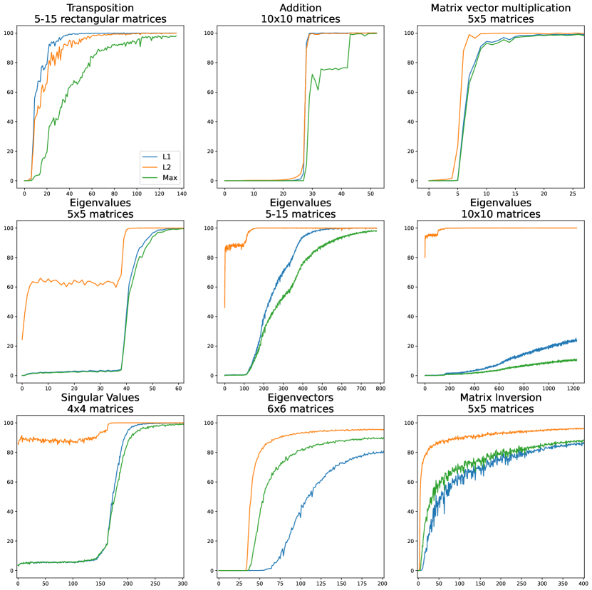
Figure 1: Learning accuracies for different problems measured with norms $L^{1}$, $L^{2}$and $L^{\infty}$ (Max).

Appendix B $L^{1}$, $L^{2}$ and $L^{\infty}$ norms for evaluation

The accuracy of trained models is evaluated by decoding their predictions and verifying that they approximate the correct solution up to a fixed tolerance $\tau$. In the general case, if the model predicts a sequence $S_{P}$, and the solution of the problem is $O$, the prediction is considered to be correct if $S_{P}$ can be decoded into a matrix $P$ and

$$\|P-O\|<\tau\|O\|$$ (1)

For eigenvalue decomposition, the solution is correct if it can be decomposed as a pair $(Q,D)$ that verifies: $\|Q^{T}IQ-D\|<\tau\|D\|$ ($I$ the input matrix), i.e. that $Q$ diagonalizes $I$ into $D$. For singular value decomposition, the solution must verify $\|UIV-S\|<\tau\|S\|$, and for matrix inversion $\|PI-Id\|<\tau\|Id\|=\tau$. The matrix norm $L^{1}$: $\|A\|=\sum_{i,j}{|a_{i,j}|}$, for $A=(a_{i,j})$ is used throughout this paper. This section discusses its advantage over two other possible norms: $L^{2}$ ($\|A\|=\sum_{i,j}{a_{i,j}^{2}}$), and $L^{\infty}$ ($\|A\|=\max_{i,j}{|a_{i,j}|}$).

Using $L^{1}$ norm in equation 1 amounts to comparing the average absolute error on the predicted coefficients ($P-O$) to the average absolute value of coefficients of $O$. $L^{2}$ compares the squared values and errors, and $L^{\infty}$ the largest absolute error to the largest coefficient in $|O|$. Compared to $L^{1}$, $L^{2}$ and $L^{\infty}$ (Max) emphasize large absolute errors, and large absolute coefficients of $O$. The impact of the norm varies from one problem to another. Figure 1 presents learning curves using the three norms for our best models, on different problems.

For basic arithmetic operations (transposition, addition, multiplication), there is little difference between $L^{1}$ and $L^{2}$ accuracies, and no reason to prefer one over the other for model evaluation. $L^{\infty}$ provides a stricter criterion for accuracy, but it has little practical impact.

For eigenvalue and singular value problems, $L^{2}$ accuracies reach a high value early during training, long before the model begins to learn according to the other norms. This is due to the fact that the eigenvalues of Wigner matrices tend to be regularly spaced over the interval $[-2\sigma,2\sigma]$ ($\sigma=\sqrt{n}s$ with $s$ the standard deviation of coefficients and $n$ the dimension of the matrix). This means that the model can predict the largest absolute eigenvalues from the distribution of the coefficients, which can be computed from the dataset. For this reason, $L^{2}$ accuracy is not a good evaluation metric for the eigenvalue or singular value problem. This is particularly clear in the $10\times 10$ case: transformers struggle with such matrices, and $L^{1}$ and $L^{\infty}$ accuracies remain very low even after a thousand epochs (300 million examples), but $L^{2}$ accuracy is close to $100\%$ since the beginning of training.

A similar phenomenon takes place for eigenvector calculations: $L^{2}$ and $L^{\infty}$ accuracy rise steeply, long before the model begins to learn according to the $L^{1}$ norm. In this task, the model predicts both the eigenvalues and the coefficients of the matrix of eigenvectors $Q$. Because $Q$ is orthogonal, its coefficients will usually have small absolute values, compared to those of eigenvalues. As training goes on, the largest eigenvalue is first predicted, which causes the rise in the $L^{2}$ curve, then other eigenvalues are, which cause the rise in the $L^{\infty}$ curve, and finally the eigenvectors are correctly predicted, which is depicted in the (much slower) rise of the $L^{1}$ curve. Again, using $L^{2}$ or $L^{\infty}$ amounts to evaluating an easier problem (computing eigenvalues) than the one we are currently solving (eigen decomposition). These observations motivate the choice of $L^{1}$ as our evaluation norm.

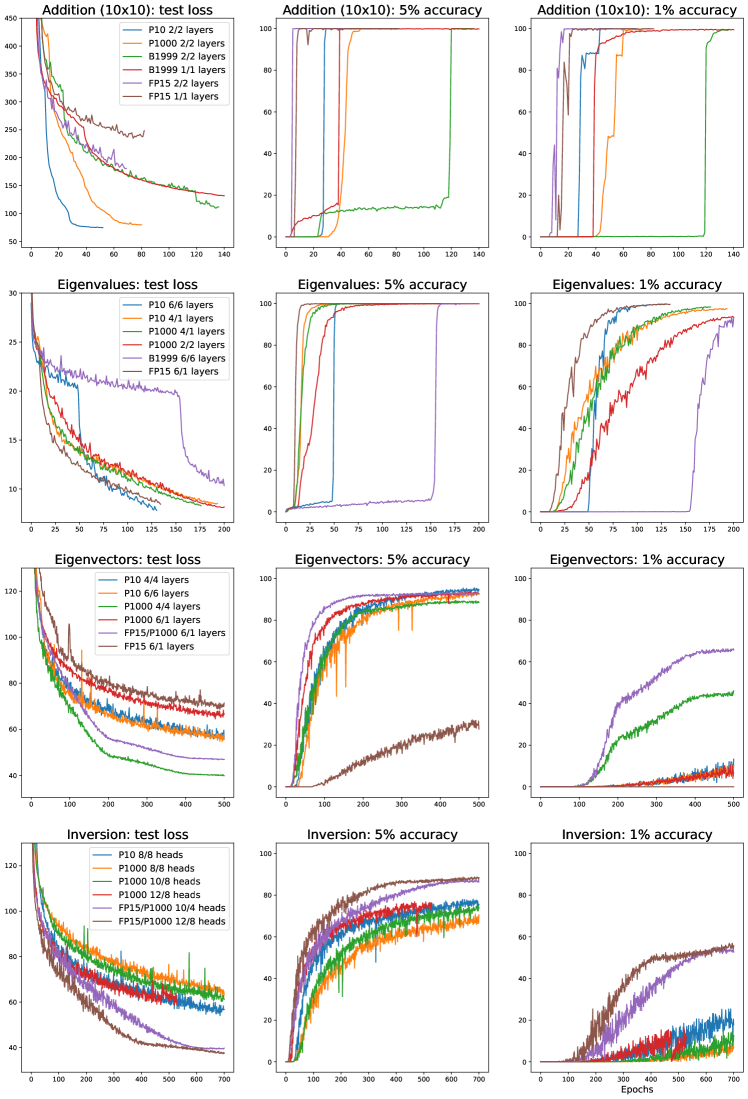
Figure 2: Learning curves for different problems. All problems except addition use $5\times 5$ matrices. All models have $512$ dimensions and $8/8$ heads (except when mentioned in the legend). Inversion models have $6/1$ layers. Epochs correspond to 300,000 training examples. Test loss is cross-entropy.

Appendix C Impact of number precision

In all experiments, matrix coefficients are rounded to three significant digits. Three-digit precision was selected in order to keep the size of the FP15 vocabulary manageable. With three-digit precision, FP15 uses a vocabulary of 30 000 words, with four digits, it would use 300 000 words, and would be difficult to train on the small transformers this paper focuses on.

In this section, I investigate the impact of number precision on $10\times 10$ matrix addition and $5\times 5$ eigenvalue computation. Random matrices are rounded to two, three and four significant digits, using the P100, P1000 and P10000 encoding (i.e. numbers encoded on three tokens, mantissa in base 100, 1000 and 10000). I train transformers with 512 dimensions, 8 attention heads, and 2/2 layers (addition) or 4/1 layers (eigenvalues). Results for $10$, $5$, $2$, $1$, $0.5$ and $0.1\%$ tolerance are presented in tables 13 and 14.

On the addition task, rounding precision has no impact for tolerances larger than $1\%$: all models achieve close to $100\%$ accuracy. At $0.5$ tolerance, models trained with 2-digit precision are penalised by rounding error, but there is no significant difference between 3 and 4-digit precision. However, 4-digit models need significantly more examples to train: whereas 2 and 3-digit models achieve $99\%$ accuracy at $5\%$ tolerance after $5$ million examples, a 4-digit model need $21$ millions to reach $99\%$ accuracy.

Tolerance	10	5	2	1	0.5	0.1
2-digit precision, P100	100	100	100	99.4	60.8	0
3-digit precision, P1000	100	100	99.3	98.1	97.2	66.4
4-digit precision, P10000	99.5	99.4	99.4	99.0	98.8	17.3

Table 13: Accuracy of $10\times 10$ matrix addition, for different precision and tolerance, after training on $30$ million examples.

For eigenvalues, all models achieve $100\%$ accuracy at $5\%$ tolerance. At lower tolerance ($1$ or $0.5\%$), accuracy increases with precision. On this task, learning speed is comparable for all models: 2, 3 and 4-digit models achieve $99\%$ accuracy (with $5\%$ tolerance) after 9, 8 and 7 million examples respectively. Overall, number precision has a marginal effect on accuracy.

Tolerance	10	5	2	1	0.5	0.1
2-digit precision, P100	100	100	94.3	87.4	80.1	24.1
3-digit precision, P1000	100	100	99.9	98.2	78.9	9.8
4-digit precision, P10000	100	100	99.9	99.0	85.6	1.4

Table 14: Accuracy of $5\times 5$ eigenvalue calculation, for different precision and tolerance, after training on $60$ million examples.

Appendix D Additional experimental results

D.1 Learning curves for different encodings and architectures

Figure 2 presents learning curves (test loss, $5$ and $1\%$ accuracy) for ($10\times 10$) addition, and ($5\times 5$eigenvalues, eigenvectors and inversion. The best models learn to perform addition ($1\%$ tolerance) in less than $10$ epochs ($3$ million examples). For other tasks, training size increases with operation complexity: from $20$ million (70 epochs) for eigenvalues, to $50$ million for eigenvectors, and over $120$ million for matrix inversion. Some of the learning curves exhibit the “step shapes” often observed in arithmetic tasks: losses are subject to brutal drops, corresponding to steep increases in accuracy.

The learning curves for the harder problems (eigenvalues, eigenvectors and inversion) are noisy. This is caused by the learning rates: our models usually need small learning rates ($5\times 10^{-4}$ before scheduling is typical) and there is a trade-off between low rates that will stabilize the learning curve, and larger rates that accelerate training.

D.2 Impact of model size on accuracy and learning speed

Two main factors influence model size: the number of layers and the number of dimensions (see Appendix G for precise calculations). This section discusses their impact on accuracy and learning speed, when adding $10\times 10$ matrices, multiplying a $5\times 5$ matrix by a vector, and computing the eigenvalues of a $5\times 5$ matrix. All the models in this section are symmetric (same dimension and number of layers in the encoder and decoder) and have $8$ attention heads.

For the addition task, tables 15 and 16 present the accuracy after 60 epochs (18 million examples) and the number of epochs (of 300,000 examples) needed to reach $95\%$ accuracy, for models using the P1000 and B1999 encoding. Shallow architectures (i.e. 1 or 2 layers) learn addition with high accuracy for both encodings, but the more compact B1999 supports smaller models ($256$ dimensions). In terms of speed, shallow (2-layer) B1999 and deep (6-layer) P100 prove fastest.

	B1999				P1000
dimension	64	128	256	512	64	128	256	512
1/1 layers	31	7	82	100	0	0	1	40
2/2 layers	0	0	100	100	0	0	0	99
4/4 layers	0	0	0	14	0	0	0	98
6/6 layers	0	0	0	0	0	0	0	99

Table 15: Accuracy of matrix addition for different model sizes. $10\times 10$ matrices, 60 epochs (18 millions examples), $5\%$ tolerance.

	B1999				P1000
dimension	64	128	256	512	64	128	256	512
1/1 layers	-	-	76	15	-	-	-	96
2/2 layers	-	-	26	6	-	-	-	37
4/4 layers	-	-	70	63	-	-	-	53
6/6 layers	-	-	-	-	-	-	-	23

Table 16: Learning speed of matrix addition for different model sizes. Number of epochs needed to reach $95\%$ accuracy ($5\%$ tolerance). 1 epoch = 300,000 examples.

Table 17 presents the learning speed of models of different sizes for the matrix/vector product and eigenvalue computation tasks ($5\times 5$ matrices, and P1000 encoding). For each problem, there exists a minimal dimension and depth under which models struggle to learn: one layer and 128 dimensions for products, one layer or 128 dimensions for eigenvalues. Over that limit, increasing the dimension accelerates learning. Increasing the depth, on the other hand, bring no clear improvement in speed or accuracy.

	Matrix product			Eigenvalues
	128	256	512	128	256	512	1024
1/1 layers	-	29	18	-	-	-	-
2/2 layers	24	12	7	-	102	36	23
4/4 layers	28	11	5	244	90	24	13
6/6 layers	24	10	6	-	-	129	16
8/8 layers	18	12	6	-	-	34	24

Table 17: Learning speed of matrix and vector products and eigenvalue calculations for different model sizes. Number of epochs needed to reach $95\%$ accuracy (with $5\%$ tolerance). 1 epoch = 300,000 examples. $5\times 5$ matrices, P1000 encoding.

D.3 Scaling to larger models

This paper mostly focuses on small models, with up to $6$ layers and $50$ million parameters. In this section, I investigate the performance of larger models, with up to $24$ layers and over $400$ million parameters. All models are asymmetric, featuring either a deep encoder and a shallow ($1$-layer) decoder, or the reverse. Shallow models have one layer, $512$ dimensions and $8$ attention heads. Deep models range from small ($6$ layers) to medium ($8$ layers), large ($12$ layers) and extra-large ($24$ layers). By default, they have a dimension of $512,640,768$ and $1024$, and $8,10,12$ and $16$ heads respectively. For each size, I also experiment with models with $50\%$ more dimensions and attention heads. The basic encoding is FP15/P1000, but I also experiment with two alternative configurations: FP15/FP15 and P1000/P1000. Table 18 summarizes the configurations that were tested.

Model size	Base configuration	Larger dimension	More heads
Small: 6 layers	512 dimensions, 8 heads	768	12
Medium: 8 layers	640 dimensions, 10 heads	960	15
Large: 12 layers	768 dimensions, 12 heads	1152	18
Extra-large: 24 layers	1024 dimensions, 16 heads	1536	24

Table 18: Large model configurations. All three configurations are tested for the encoder and decoder, and with the three encodings: FP15/P1000, P1000/P1000, FP15/FP15.

For the eigenvalue task, models are trained on $8\times 8$, $10\times 10$ and $12\times 12$ matrices. Table 19 presents the best performing configurations, for different tolerance levels, and the sample size needed to achieve $99\%$ accuracy (with $5\%$ tolerance). In general, architectures combining a deep decoder with a shallow encoder outperform deep encoders and shallow decoders. Deeper models tend to learn faster, and solve larger problems, but for a given number of layers, there is not clear advantage of increasing dimension or the number of attention heads. In particular, models with 12 or 24 layers can compute the eigenvalues of $12\times 12$ matrices, a task inaccessible to small architectures. Learning to predict the eigenvalues of $8\times 8$ matrices takes over $50$ million examples for 6-layer models, but only $11$ million for 24-layer architectures. For $10\times 10$ matrices, 8-layer models need about $85$ million examples, whereas 12 and 24-layer models need $38$ and $36$. Finally, it is interesting to note that larger models achieve better precision: 12-layer models routinely achieve accuracies over $90\%$ with $0.5\%$ tolerance, while smaller models struggle at such precision levels.

Model	Dimensions	5%	2%	1%	0.5%	Sample size*
Small (6 layers)
E:1/512/8/FP15 D:6/516/12/P1000	8x8	100	99.5	88.8	35.9	51
E:1/512/8/FP15 D:6/512/8/P1000	8x8	100	97.7	86.5	50.3	64.2
E:6/768/8/P1000 D:1/512/8/P1000	8x8	100	98.8	80.8	28.1	64.8
E:1/512/8/FP15 D:6/768/8/P1000	8x8	100	97.9	69.8	17.7	71.7
E:1/512/8/FP15 D:6/516/12/P1000	10x10	99.7	72.6	22.3	2.2	194.7
E:1/512/8/FP15 D:6/768/8/FP15	10x10	83.6	17.0	1.5	0.1	-
Medium (8 layers)
E:8/640/10/P1000 D:1/512/8/P1000	8x8	99.4	99.0	97.0	60.1	120.9
E:1/512/8/FP15 D:8/645/15/P1000	8x8	100	99.9	95.9	56.1	45
E:1/512/8/FP15 D:8/960/10/P1000	8x8	100	99.9	95.4	55.9	34.8
E:1/512/8/FP15 D:8/640/10/P1000	8x8	100	99.8	92.0	42.0	43.8
E:1/512/8/FP15 D:8/640/10/P1000	10x10	100	98.4	70.2	11.2	85.2
E:1/512/8/FP15 D:8/645/15/P1000	10x10	99.1	62.9	14.1	1.0	108.6
E:1/512/8/FP15 D:8/645/15/FP15	12x12	3.0	0	0	0	-
Large (12 layers)
E:1/512/8/FP15 D:12/1152/12/P1000	8x8	100	100	100	99.1	13.2
E:1/512/8/FP15 D:12/768/12/P1000	8x8	100	100	99.9	93.5	42
E:1/512/8/FP15 D:12/768/12/P1000	10x10	100	100	99.8	89.3	68.7
E:1/512/8/FP15 D:12/1152/12/P1000	10x10	100	100	99.7	96.8	37.5
E:1/512/8/FP15 D:12/768/12/P1000	12x12	96.7	24.2	1.5	0.1	-
E:1/512/8/FP15 D:12/768/12/FP15	12x12	85.2	11.8	0.6	0	-
Extra-large (24 layers)
E:1/512/8/FP15 D:24/1024/16/P1000	8x8	100	100	100	99.2	11.1
E:1/512/8/FP15 D:24/1032/24/P1000	8x8	100	100	100	93.9	14.1
E:1/512/8/FP15 D:24/1032/24/FP15	8x8	100	100	99.7	82.6	19.5
E:1/512/8/FP15 D:24/1024/16/P1000	10x10	100	100	99.6	75.9	36.3
E:1/512/8/FP15 D:24/1032/24/P1000	10x10	100	100	99.5	69.3	42.6
E:1/512/8/FP15 D:24/1032/24/P1000	12x12	100	99.6	95.5	43.7	99.6
E:1/512/8/FP15 D:24/1024/16/P1000	12x12	100	99.6	88.9	23.0	99.3

Table 19: Large models: accuracy of eigenvalue computations. E=Encoder, D=Decoder, 1/512/8 : 1 later, 512 dimensions, 8 heads. Sorted by 1% accuracy. *Millions of examples to reach 99% accuracy

D.4 Model performance on different training sets

The models presented in the main part of this paper are trained on Wigner matrices (matrices with independent and identically distributed, iid, coefficients) with fixed-range coefficient. In section 5, I argued that different training sets allowed for better out-of-domain generalization. Table 20 summarizes in-domain performance (i.e. accuracy when the test set is has the same distribution as the training set) on different training sets.

Wigner matrices with uniform or Gaussian distributed, and fixed or variable-range, coefficients are learned to high accuracy (more than $99\%$) by all models. The eigenvalues of non-Wigner matrices with Gaussian or Laplace distributed eigenvalues, and of mixtures of Wigner and non-Wigner matrices, are also predicted to high accuracy by all models. Over matrices with positive or uniformly distributed eigenvalues, smaller models using the FP15 encoding prove difficult to train.

	FP15		P1000
	4/1 layers	6/1 layers	4/1 layers	6/1 layers
Wigner matrices (iid coefficients)
Uniform iid A=10	99.6	100	99.8	100
Gaussian iid A=10	99.8	100	99.8	100
Uniform iid A=1,100	99.0	99.2	99.8	100
Uniform iid A=1,1000	99.2	99.5	99.7	99.8
Non Wigner
Positive A=10	12.7	100	100	100
Uniform A=10	8.2	10.8	99.9	100
Gaussian A=10	99.6	100	100	100
Laplace A=10	99.4	99.9	99.9	99.9
Gaussian+uniform+Laplace A=10	3.8	99.8	99.6	99.9
Wigner and non-Wigner mixtures
iid+gaussian A=10	99.5	99.9	98.0	99.7
iid+positive A=10	99.8	99.9	99.8	99.8
iid+Laplace A=10	99.6	99.8	99.6	99.5
iid+positive+gaussian A=10	99.8	99.9	99.7	99.9
iid+positive+Laplace A=10	99.0	99.8	99.6	99.8

Table 20: In-distribution eigenvalue accuracy (tolerance $2\%$) for different training distributions. All models have 512 dimensions, and 8 attention heads, and are trained on 5x5 matrices.

Appendix E Alternative architectures

E.1 Other sequence to sequence models : LSTM and GRU

I experimented with two popular recurrent architectures: long short-term memories (LSTM Hochreiter & Schmidhuber (1997)), and gated recurrent units (GRU Cho et al. (2014)), on three tasks : addition of $5\times 5$ and $10\times 10$ matrices, eigenvalues and matrix inversion of $5\times 5$ matrices. All models are sequence-to-sequence architectures: an encoder and a decoder (LSTM or GRU), with $2$ to $8$ layers, and $1024$ or $2048$ hidden dimensions. The input and output sequences, encoded as in the rest of the paper, are pre-processed (and decoded) via an embedding layer with $256$ or $512$ dimensions.

Addition, a very easy task for transformers (see section 4.2) proves difficult for LSTM and GRU. None of the models can learn addition of $10\times 10$ matrices. Some models can learn addition of $5\times 5$ matrices, but whereas transformers achieve $100\%$ accuracy for all tolerances, the best LSTM and GRU only exceed $90\%$ at $1\%$ tolerance. GRU seem to perform better than LSTM on this task, and 2-layer models perform better than 4-layer models, but transformers have a distinct advantage over LSTM and GRU for addition.

	2 layers				4 layers
Hidden dimension	1024		2048		1024		2048
Embedding dimension	256	512	256	512	256	512	256	512
Long short-term memory
$5\%$ tolerance	100	0	0	100	0	0	0	0
$2\%$ tolerance	98	0	0	100	0	0	0	0
$1\%$ tolerance	95	0	0	86	0	0	0	0
$0.5\%$ tolerance	34	0	0	1	0	0	0	0
Gated recurrent Units
$5\%$ tolerance	100	100	0	100	0	100	0	0
$2\%$ tolerance	100	28	0	100	0	99	0	0
$1\%$ tolerance	44	0	0	91	0	74	0	0
$0.5\%$ tolerance	0	0	0	9	0	4	0	0

Table 21: $5\times 5$ matrix addition using LSTM and GRU.

Both LSTM and GRU can be trained to predict eigenvalues of $5\times 5$ matrices with the same accuracy as transformers, for the P1000 and FP15 encoding (table 22). Matrix inversion, on the other hand, cannot be learned. Overall, these experiments show that other sequence to sequence architectures, LSTM and GRU, can learn tasks like eigenvalues and addition of small matrices. However, they are less efficient on addition (in terms of precision and scaling to larger matrices) and fail on more complex tasks, like matrix inversion.

	FP15						P1000
Hidden dimension	1024			2048			1024			2048
Layers	4	6	8	4	6	8	4	6	8	4	6	8
LSTM
$5\%$ tolerance	100	100	100	100	100	6	100	100	5	100	100	100
$2\%$ tolerance	95	100	100	99	100	1	100	100	1	100	99	100
$1\%$ tolerance	78	98	99	91	98	0	97	98	0	100	92	99
$0.5\%$ tolerance	46	81	83	62	68	0	78	88	0	89	57	76
Gated recurrent Units
$5\%$ tolerance	100	100	100	100	100	100	100	100	100	100	5	100
$2\%$ tolerance	98	99	100	100	100	100	99	100	100	100	1	100
$1\%$ tolerance	86	93	96	98	99	97	94	98	95	97	0	98
$0.5\%$ tolerance	53	68	75	78	83	65	65	76	63	75	0	66

Table 22: Eigenvalue computation with LSTM and GRU, $5\times 5$ matrices.

E.2 Shared-layer transformers: Universal transformers

In the Universal Transformer (Dehghani et al., 2018), the stacked layers of usual transformer implementations are replaced by one layer that is looped through a fixed number of times (feeding the output of one iteration into the input of the next). This amounts to sharing the weights of the different layers, therefore greatly reducing the number of parameters in the model. This technique can be applied to the encoder, the decoder or both. The number of iterations is a fixed hyperparameter, but the original paper also proposed a halting mechanism inspired by Adaptive Computation Time (Graves, 2016), to adaptively control loop length at the token level. In this version, a stopping probability is learned for every position in the input sequence, and once it reaches a certain threshold, the layer merely copies the input onto the output. The iteration stops when all positions have halted, or a specific value is reached. A recent paper (Csordás et al., 2021) proposes to use a similar copy-gating mechanism to skip iterations in a fixed-length loop. I experiment with these three variants (fixed length, adaptive halting, copy gating) on the addition (of $10\times 10$ matrices), eigenvalue and matrix inversion tasks ($5\times 5$ matrices).

For the addition task, I train universal transformers with one layer and in the encoder and decoder, $256$ or $512$ dimensions and $8$ attention heads, and use the B1999 encoding for the data. I experiment with looped encoder, looped decoder, and loop in both, a loop length of $4$, copy-gating and ACT (the 4 loops in then a maximum number of iterations)and copy-gating. Table 23 summarizes my findings. Only models with encoder loops learn to add, and models with 512 dimensions learn with over $95\%$ accuracy for all tolerances. Universal Transformers with one layer (looped-encoder only) perform as well as 2/2 transformers.

	$5\%$	$2\%$	$1\%$	$0.5\%$
Looped encoder
256 dimensions, 4 loops	15	1	0	0
512 dimensions, 4 loops	100	100	100	100
256 dimensions, 4 loops, gated	97	66	41	29
512 dimensions, 4 loops, gated	100	100	100	100
256 dimensions, 4 loops, ACT	100	92	76	66
512 dimensions, 4 loops, ACT	100	100	98	96
Looped decoder	0	0	0	0
Looped encoder and decoder	0	0	0	0
2/2 transformer (baseline)	100	100	100	100

Table 23: Accuracy of Universal transformers, $10\times 10$ matrix addition for different tolerances.

On the eigenvalue task, I experiment on the P1000 and FP15 encoding, with encoder-loop only 1/1 Universal Transformers with $4$ or $8$ loops. Universal transformers using the P1000 encoding achieve the same performances (with only one layer) than transformers from section 4.4. $4$ loop transformers seem to perform best, gating does not seem to improve performance and ACT slightly degrades it. With the FP15 encoding, universal transformers become very difficult to train: only the 4 loop gated version achieves significant accuracy (still lower than the 6/1 transformers).

	$5\%$	$2\%$	$1\%$	$0.5\%$
P1000
4 loops	100	100	97	87
8 loops	100	99	93	69
4 loops, gated	100	100	98	91
8 loops, gated	100	100	99	90
4 loops, ACT	100	97	89	62
8 loops, ACT	100	95	77	42
FP15
4 loops	4	0	0	0
8 loops	0	0	0	0
4 loops, gated	94	84	57	23
8 loops, gated	6	1	0	0
4 loops, ACT	4	0	0	0
8 loops, ACT	4	0	0	0
4/1 transformer (P1000 baseline)	100	100	99	89
6/1 transformer (FP15 baseline)	100	100	100	92

Table 24: Accuracy of Universal transformers, $5\times 5$ matrices eigenvalue computation for different tolerances.

Finally, I experimented with matrix inversion, with FP15/P1000 and P1000/P1000 encodings, and 4 or 8 loops in the encoder. A gated universal transformer using FP15 in the input and P1000 in the output achieved $73\%$ accuracy, a significant result albeit lower than the best result achieved with $6/1$ transformers using the same encodings ($90\%$). With the P1000 encoding, the best universal transformers reach $55\%$ accuracy, compared to $80\%$ for their $6/1$ transformer counterparts. Overall, Universal Transformers seem to achieve comparable performances with deep transformers (except on the inversion tasks), using less parameters. This makes shared layer transformers an interesting direction for future work.

Appendix F Additional experiments

F.1 Retraining

Models trained on matrices of a given size do not generalize to different dimensions, but they can be retrained over samples of matrices of different size. This takes comparatively few examples: a $5\times 5$ model, that takes $40$ million examples to be trained, can learn to predict with high accuracy eigenvalues of matrices of dimension $6$ and $7$ with about $25$ million additional examples. Table 25 presents those results. The possibility to retrain large transformers (such as GPT-3) on different tasks is well documented, it is interesting to observe the same phenomenon in smaller models.

Encoding	Retrain dimensions	Accuracy ($5\%$)	Accuracy ($2\%$)	Retrain examples
P10	5-6	100	99.9	10M
P10	5-7	100	93.6	25M
P1000	5-6	100	97.7	25M

Table 25: Model accuracy after retraining. Models trained over 5x5 matrices, retrained over 5-6 and 5-7. Overall performance after retraining (tolerance $5$ and $2\%$), and number of examples needed for retraining. All models have 512 dimensions and 8 attention heads

F.2 Joint training: learning to perform several operations

All models so far are trained on just one task. In this section, I investigate joint learning: training one model to perform several operations. To this effect, a token is added at the beginning of the input and output sequence, to indicate the task (e.g. Transpose or Add), and generate training data by randomly mixing examples of the different operations to be performed.

Transformers with $4$ or $6$ layers, $512$ dimensions and $8$ attention heads are trained on eight datasets corresponding to the following joint training goals (all operations in equal proportions):

• Transpose and add (TA)

• Transpose, add and dot product (vector matrix multiplication) (TAD)

• Transpose, add, dot product and matrix multiplication (TADM)

• Transpose, add, dot product, matrix multiplication and eigenvalues (TADME)

• Transpose, add, dot product, matrix multiplication, eigenvalues and eigenvectors (TADMEF)

• Transpose, add, dot product, matrix multiplication, eigenvalues, eigenvectors and matrix inversion (TADMEFI)

• Eigenvalues, eigenvectors and matrix inversion (EFI)

Table 26 summarizes results.

	T	A	D	M	E	F	I
TA	100	100
TAD	100	100	100
TADM	100	100	100	100
TADME	100	100	26	100	80
TADMEF	100	100	100	100	3	0
TADMEFI	100	100	100	100	3	0	0
EFI					100	22	0

Table 26: Accuracy of joint training, $5\times 5$ matrices, $5\%$ tolerance.

Over mixtures of the four basic operations (transposition, addition, dot products and multiplication: goals TA, TAD and TADM), models predict all operations with almost perfect accuracy. Joint training on the basic operations and eigenvalue computations (the TADME task) allows the model to predict eigenvalues with $80\%$ accuracy, in exchange for a loss of performances on the dot product task. As the number of non-basic tasks increases, the model keeps learning basic operations to $100\%$ accuracy (as in the TADM setting), but the more advanced operations are not learned. Joint training on the advanced tasks only (eigenvalues, vectors and inversion) results in $100\%$ accuracy on eigenvalue computation, $22\%$ on eigenvectors, and $0$ on inversion. These results demonstrate the feasibility of joint training on basic matrix operations, but also suggest that further research is needed if one wants to extend joint training to all the tasks considered in this paper.

F.3 Additional results with noisy data

See tables 27 and 28.

	B1999				P1000
	2/2 layers		4/4 layers		2/2 layers		4/4 layers
	256	512	256	512	256	512	256	512
$5\%$ tolerance
$0.01\sigma$ error	100	100	100	100	100	100	99.4	100
$0.02\sigma$	100	100	99.8	100	100	100	100	100
$0.05\sigma$	41.5	41.2	41.7	41.6	39.3	41.2	39.4	40.7
$2\%$ tolerance
$0.01\sigma$ error	99.8	99.9	99.8	99.9	99.4	100	98.2	99.9
$0.02\sigma$	43.7	44.2	42.1	44.7	39.0	44.9	42.6	45.3
$0.05\sigma$	0	0	0	0	0	0	0	0
$1\%$ tolerance
$0.01\sigma$ error	39.8	41.7	39.6	44.0	36.6	44.0	28.9	44.6
$0.02\sigma$	0.1	0.1	0.1	0.1	0.1	0.1	0.1	0.1
$0.05\sigma$	0	0	0	0	0	0	0	0

Table 27: Accuracy of noisy $5\times 5$ matrix addition for different error levels and tolerances.

	FP15				P1000
	4/4 layers		6/6 layers		4/4 layers		6/6 layers
	512	1024	512	1024	512	1024	512	1024
$5\%$ tolerance
$0.01\sigma$ error	6.1	100	5.1	6.0	100	100	100	100
$0.02\sigma$	100	100	6.7	100	100	100	100	100
$0.05\sigma$	99.1	99.3	99.3	6.4	99.3	99.0	99.0	98.8
$2\%$ tolerance
$0.01\sigma$ error	0.7	99.8	0.5	0.8	99.3	99.6	99.9	99.8
$0.02\sigma$	97.0	97.1	0.8	88.4	97.3	97.9	93.1	95.4
$0.05\sigma$	37.9	38.4	40.6	0.5	40.1	37.3	37.5	35.3
$1\%$ tolerance
$0.01\sigma$ error	0.1	82.1	0.1	0.2	79.7	83.8	87.9	83.8
$0.02\sigma$	47.8	51.3	0.1	26.1	46.2	47.5	36.4	41.3
$0.05\sigma$	3.8	4.2	4.1	0.1	4.1	3.8	3.9	3.4

Table 28: Accuracy of noisy eigenvalue computations, for different error levels and tolerances, $5\times 5$ matrices.

Appendix G Number of parameters

The number of parameters in the sequence-to-sequence transformers used in this paper can be calculated as follows.

• A self-attention mechanism with dimension $d$ has $4d(d+1)$ parameters: it is composed of four linear layers (K, Q, V and the output layer), with $d$ input, $d$ output and a bias.

• A cross-attention mechanism with $d_{e}$ dimensions in the encoder, and $d$ in the decoder has $2d(d+d_{e}+2)$ parameters (K and V are $d_{e}\times d$ layers).

• A FFN with one hidden layer, $d$ input and output, and $h$ hidden units has $d(h+1)+h(d+1)$ parameters.

• A layer normalization with $d$ dimensions has $2d$ parameters.

• An encoder layer with dimension $d$ has a self-attention mechanism, a FFN with $4d$ hidden units (in this implementation) and two layer normalizations, for a total number of parameters of $12d^{2}+13d$.

• A decoder layer has a cross-attention layer (encoding dimension $d_{e}$) and a layer normalization on top of an encoder, for a total of $14d^{2}+19d+2d_{e}d$ parameters.

• An embedding of dimension $d$ for a vocabulary of $w$ words will use $dw$ parameters, and $2d$ more if it is coupled to a layer normalization.

• The final prediction layer with an output dimension of $d$ and a decoded vocabulary of $w$ words will use $(d+1)w$ parameters (but in this case, $dw$ will be shared with the decoder embedding).

Overall, the number of parameters for a transformer with $n_{e}$ encoding layers with dimension $d_{e}$, $n*d$ decoding layers with dimension $d_{d}$, an input vocabulary of $w_{i}$ words, an output vocabulary of $w_{o}$ words and a positional embedding of $w_{p}$ words (corresponding to the maximum sequence length) can be computed by the formula:

$$P=d_{e}(w_{i}+w_{p}+2)+((w_{o}+w_{p}+2)d_{d}+w_{o})+n_{e}d_{e}(12d_{e}+13)+n_{d}d_{d}(14d_{d}+2d_{e}+19)$$

the four terms in the sum corresponding to the input embedding, the output embedding, the encoder and the decoder.

Table 29 provides the number of parameters for some of the models used in this paper. For the positional embedding, the number of words is the longest input and output sequence studied with that model.

Experiment	Model	Parameters
Transposition	1/1 layers 256 dimensions P10	2,276,171
	1/1 layers 256 dimensions P1000	2,737,871
	1/1 layers 256 dimensions B1999	3,297,554
	1/1 layers 256 dimensions FP15	17,045,441
Addition	2/2 layers, 512 dimensions, B1999	17,619,218
Matrix vector multiplication	2/2 layers 512 dimensions P10	15,578,443
	2/2 layers 512 dimensions P1000	16,500,943
	4/4 layers 512 dimensions P1000	31,213,775
Matrix multiplication	1/4 layers 512 dimensions P1000	21,756,623
	1/6 layers 512 dimensions P1000	30,164,687
Eigen decomposition	1/6 layers 512 dimensions FP15	58,751,937
	6/1 layers 512 dimensions FP15	53,493,697
	6/1 layers 512 dimensions P1000	24,906,447
	6/6 layers 512 dimensions P1000	45,926,607
Matrix inversion	6/1 layers 512 dimensions FP15/P1000	39,186,127

Table 29: Number of parameters of transformers used in the paper.

Appendix H Eigenvalue distribution of Wigner matrices, an empirical justification

Figure 3 provides an empirical confirmation of the property of Wigner matrices mentioned in sections 2.2 and 5: the standard deviation of their eigenvalues is a function of their dimension and standard deviation of their coefficients only, and does not depend on the actual distribution of the coefficients. In particular, for coefficients with standard deviation $\sigma=10/\sqrt{3}=5.77$, we expect the standard deviation of their eigenvalue distribution to be $\sigma=12.91,18.26,22.36$ and $25.81$ for square matrices of dimension $5,10,15$ and $20$.

For three distributions, uniform, Laplace and gaussian, and four dimensions ($5,10,15$, and $20$), 100 000 random matrices with the same standard deviation of coefficients were generated, and their eigenvalues were computed. Standard deviations are within $0.01$ of theoretical values for all distributions and dimensions. It is interesting to note how the distributions (which correspond to the original coefficient distribution for $n=1$) are similar to the semi-circle as dimension increases.

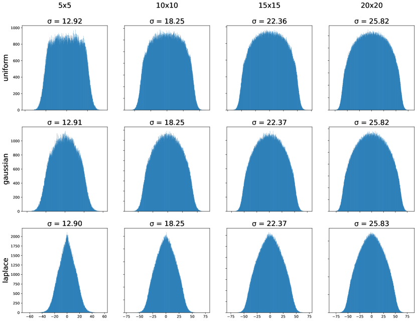
Figure 3: Empirical distributions of eigenvalues for Wigner matrices, dimension 5x5 (left) to 20x20 (right), with uniform (top), gaussian (middle) and Laplace (bottom) coefficients. All distributions computed from 100 000 random matrices.

References

- Biggio et al. (2021) Luca Biggio, Tommaso Bendinelli, Alexander Neitz, Aurelien Lucchi, and Giambattista Parascandolo. Neural symbolic regression that scales. arXiv preprint arXiv:2106.06427, 2021.
- Blalock & Guttag (2021) Davis Blalock and John Guttag. Multiplying matrices without multiplying. arXiv preprint arXiv:2106.10860, 2021.
- Bommasani et al. (2021) Rishi Bommasani, Drew A. Hudson, Ehsan Adeli, Russ Altman, Simran Arora, Sydney von Arx, Michael S. Bernstein, Jeannette Bohg, Antoine Bosselut, Emma Brunskill, Erik Brynjolfsson, Shyamal Buch, Dallas Card, Rodrigo Castellon, Niladri Chatterji, Annie Chen, Kathleen Creel, Jared Quincy Davis, Dora Demszky, Chris Donahue, Moussa Doumbouya, Esin Durmus, Stefano Ermon, John Etchemendy, Kawin Ethayarajh, Li Fei-Fei, Chelsea Finn, Trevor Gale, Lauren Gillespie, Karan Goel, Noah Goodman, Shelby Grossman, Neel Guha, Tatsunori Hashimoto, Peter Henderson, John Hewitt, Daniel E. Ho, Jenny Hong, Kyle Hsu, Jing Huang, Thomas Icard, Saahil Jain, Dan Jurafsky, Pratyusha Kalluri, Siddharth Karamcheti, Geoff Keeling, Fereshte Khani, Omar Khattab, Pang Wei Koh, Mark Krass, Ranjay Krishna, Rohith Kuditipudi, Ananya Kumar, Faisal Ladhak, Mina Lee, Tony Lee, Jure Leskovec, Isabelle Levent, Xiang Lisa Li, Xuechen Li, Tengyu Ma, Ali Malik, Christopher D. Manning, Suvir Mirchandani, Eric Mitchell, Zanele Munyikwa, Suraj Nair, Avanika Narayan, Deepak Narayanan, Ben Newman, Allen Nie, Juan Carlos Niebles, Hamed Nilforoshan, Julian Nyarko, Giray Ogut, Laurel Orr, Isabel Papadimitriou, Joon Sung Park, Chris Piech, Eva Portelance, Christopher Potts, Aditi Raghunathan, Rob Reich, Hongyu Ren, Frieda Rong, Yusuf Roohani, Camilo Ruiz, Jack Ryan, Christopher Ré, Dorsa Sadigh, Shiori Sagawa, Keshav Santhanam, Andy Shih, Krishnan Srinivasan, Alex Tamkin, Rohan Taori, Armin W. Thomas, Florian Tramèr, Rose E. Wang, William Wang, Bohan Wu, Jiajun Wu, Yuhuai Wu, Sang Michael Xie, Michihiro Yasunaga, Jiaxuan You, Matei Zaharia, Michael Zhang, Tianyi Zhang, Xikun Zhang, Yuhui Zhang, Lucia Zheng, Kaitlyn Zhou, and Percy Liang. On the opportunities and risks of foundation models, 2021.
- Brockett (1991) Roger W Brockett. Dynamical systems that sort lists, diagonalize matrices, and solve linear programming problems. Linear Algebra and its applications, 146:79–91, 1991.
- Cappart et al. (2021) Quentin Cappart, Didier Chételat, Elias Khalil, Andrea Lodi, Christopher Morris, and Petar Veličković. Combinatorial optimization and reasoning with graph neural networks, 2021.
- Carion et al. (2020) Nicolas Carion, Francisco Massa, Gabriel Synnaeve, Nicolas Usunier, Alexander Kirillov, and Sergey Zagoruyko. End-to-end object detection with transformers. arXiv preprint arXiv:2005.12872, 2020.
- Castellini (2019) Jacopo Castellini. Learning numeracy: Binary arithmetic with neural turing machines. arXiv preprint arXiv:1904.02478, 2019.
- Charton et al. (2020) François Charton, Amaury Hayat, and Guillaume Lample. Learning advanced mathematical computations from examples. arXiv preprint arXiv:2006.06462, 2020.
- Child et al. (2019) Rewon Child, Scott Gray, Alec Radford, and Ilya Sutskever. Generating long sequences with sparse transformers. arXiv preprint arXiv:1904.10509, 2019.
- Cho et al. (2014) Kyunghyun Cho, Bart Van Merriënboer, Caglar Gulcehre, Dzmitry Bahdanau, Fethi Bougares, Holger Schwenk, and Yoshua Bengio. Learning phrase representations using rnn encoder-decoder for statistical machine translation. arXiv preprint arXiv:1406.1078, 2014.
- Cichocki & Unbehauen (1992) Andrzej Cichocki and Rolf Unbehauen. Neural networks for computing eigenvalues and eigenvectors. Biological Cybernetics, 68(2):155–164, 1992.
- Cobbe et al. (2021) Karl Cobbe, Vineet Kosaraju, Mohammad Bavarian, Jacob Hilton, Reiichiro Nakano, Christopher Hesse, and John Schulman. Training verifiers to solve math word problems. arXiv preprint arXiv:2110.14168, 2021.
- Csordás et al. (2021) Róbert Csordás, Kazuki Irie, and Jürgen Schmidhuber. The neural data router: Adaptive control flow in transformers improves systematic generalization. arXiv preprint arXiv:2110.07732, 2021.
- Cybenko (1989) George Cybenko. Approximation by superpositions of a sigmoidal function. Mathematics of control, signals and systems, 2(4):303–314, 1989.
- d’Ascoli et al. (2022) Stéphane d’Ascoli, Pierre-Alexandre Kamienny, Guillaume Lample, and François Charton. Deep symbolic regression for recurrent sequences, 2022.
- Davies et al. (2021) A Davies, P Velickovic, L Buesing, S Blackwell, D Zheng, N Tomasev, R Tanburn, P Battaglia, C Blundell, A Juhasz, et al. Advancing mathematics by guiding human intuition with ai. Nature, 2021.
- Davis (2019) Ernest Davis. The use of deep learning for symbolic integration: A review of (lample and charton, 2019). arXiv preprint arxiv:1912.05752, 2019.
- Dehghani et al. (2018) Mostafa Dehghani, Stephan Gouws, Oriol Vinyals, Jakob Uszkoreit, and Łukasz Kaiser. Universal transformers. arXiv preprint arXiv:1807.03819, 2018.
- Dersy et al. (2022) Aurélien Dersy, Matthew D. Schwartz, and Xiaoyuan Zhang. Simplifying polylogarithms with machine learning, 2022.
- Dong et al. (2018) Linhao Dong, Shuang Xu, and Bo Xu. Speech-transformer: A no-recurrence sequence-to-sequence model for speech recognition. In 2018 IEEE International Conference on Acoustics, Speech and Signal Processing (ICASSP), pp. 5884–5888, 2018.
- Dosovitskiy et al. (2021) Alexey Dosovitskiy, Lucas Beyer, Alexander Kolesnikov, Dirk Weissenborn, Xiaohua Zhai, Thomas Unterthiner, Mostafa Dehghani, Matthias Minderer, Georg Heigold, Sylvain Gelly, Jakob Uszkoreit, and Neil Houlsby. An image is worth 16x16 words: Transformers for image recognition at scale. arXiv preprint arXiv:2010.11929, 2021.
- Finol et al. (2019) David Finol, Yan Lu, Vijay Mahadevan, and Ankit Srivastava. Deep convolutional neural networks for eigenvalue problems in mechanics. International Journal for Numerical Methods in Engineering, 118(5):258–275, 2019.
- Graves (2016) Alex Graves. Adaptive computation time for recurrent neural networks. arXiv preprint arXiv:1603.08983, 2016.
- Griffith & Kalita (2021) Kaden Griffith and Jugal Kalita. Solving arithmetic word problems with transformers and preprocessing of problem text. arXiv preprint arXiv:2106.00893, 2021.
- Hahn et al. (2021) Christopher Hahn, Frederik Schmitt, Jens U. Kreber, Markus N. Rabe, and Bernd Finkbeiner. Teaching temporal logics to neural networks. arXiv preprint arXiv:2003.04218, 2021.
- Han et al. (2021) Jesse Michael Han, Jason Rute, Yuhuai Wu, Edward W. Ayers, and Stanislas Polu. Proof artifact co-training for theorem proving with language models. arXiv preprint arxiv:2102.06203, 2021.
- Hochreiter & Schmidhuber (1997) Sepp Hochreiter and Jürgen Schmidhuber. Long short-term memory. Neural computation, 9(8):1735–1780, 1997.
- Hornik (1991) Kurt Hornik. Approximation capabilities of multilayer feedforward networks. Neural networks, 4(2):251–257, 1991.
- Iakovlev et al. (2020) Valerii Iakovlev, Markus Heinonen, and Harri Lähdesmäki. Learning continuous-time pdes from sparse data with graph neural networks, 2020.
- Kaiser & Sutskever (2015) Łukasz Kaiser and Ilya Sutskever. Neural gpus learn algorithms. arXiv preprint arXiv:1511.08228, 2015.
- Kalchbrenner et al. (2015) Nal Kalchbrenner, Ivo Danihelka, and Alex Graves. Grid long short-term memory. arXiv preprint arxiv:1507.01526, 2015.
- Kingma & Ba (2014) Diederik P Kingma and Jimmy Ba. Adam: A method for stochastic optimization. arXiv preprint arXiv:1412.6980, 2014.
- Knuth (1997) Donald E. Knuth. The Art of Computer Programming, Volume 2: Seminumerical Algorithms. Addison-Wesley, third edition, 1997.
- Lample & Charton (2019) Guillaume Lample and François Charton. Deep learning for symbolic mathematics. arXiv preprint arXiv:1912.01412, 2019.
- Lewkowycz et al. (2022) Aitor Lewkowycz, Anders Andreassen, David Dohan, Ethan Dyer, Henryk Michalewski, Vinay Ramasesh, Ambrose Slone, Cem Anil, Imanol Schlag, Theo Gutman-Solo, Yuhuai Wu, Behnam Neyshabur, Guy Gur-Ari, and Vedant Misra. Solving quantitative reasoning problems with language models, 2022.
- Loshchilov & Hutter (2016) Ilya Loshchilov and Frank Hutter. Sgdr: Stochastic gradient descent with warm restarts. arXiv preprint arXiv:1608.03983, 2016.
- Mehta (2004) Madan Lal Mehta. Random Matrices. Academic Press, 3rd edition, 2004.
- Meng & Rumshisky (2019) Yuanliang Meng and Anna Rumshisky. Solving math word problems with double-decoder transformer. arXiv preprint arXiv:1908.10924, 2019.
- Nogueira et al. (2021) Rodrigo Nogueira, Zhiying Jiang, and Jimmy Lin. Investigating the limitations of transformers with simple arithmetic tasks. arXiv preprint arXiv:2102.13019, 2021.
- Oja (1992) Erkki Oja. Principal components, minor components, and linear neural networks. Neural networks, 5(6):927–935, 1992.
- Palamas (2017) Theodoros Palamas. Investigating the ability of neural networks to learn simple modular arithmetic. 2017.
- Polu & Sutskever (2020) Stanislas Polu and Ilya Sutskever. Generative language modeling for automated theorem proving. arXiv preprint arXiv:2009.03393, 2020.
- Preciado & Rahimian (2017) Victor M. Preciado and M. Amin Rahimian. Moment-based spectral analysis of random graphs with given expected degrees. arXiv preprint arXiv:1512.03489, 2017.
- Radford et al. (2018) Alec Radford, Karthik Narasimhan, Tim Salimans, and Ilya Sutskever. Improving language understanding by generative pre-training. 2018.
- Radford et al. (2019) Alec Radford, Jeffrey Wu, Rewon Child, David Luan, Dario Amodei, Ilya Sutskever, et al. Language models are unsupervised multitask learners. OpenAI blog, 1(8):9, 2019.
- Samardzija & Waterland (1991) Nikola Samardzija and RL Waterland. A neural network for computing eigenvectors and eigenvalues. Biological Cybernetics, 65(4):211–214, 1991.
- Saxton et al. (2019) David Saxton, Edward Grefenstette, Felix Hill, and Pushmeet Kohli. Analysing mathematical reasoning abilities of neural models. arXiv preprint arXiv:1904.01557, 2019.
- Scarselli et al. (2009) Franco Scarselli, Marco Gori, Ah Chung Tsoi, Markus Hagenbuchner, and Gabriele Monfardini. The graph neural network model. IEEE Transactions on Neural Networks, 20(1):61–80, 2009.
- Shalev-Shwartz et al. (2017) Shai Shalev-Shwartz, Ohad Shamir, and Shaked Shammah. Failures of gradient-based deep learning. In Doina Precup and Yee Whye Teh (eds.), Proceedings of the 34th International Conference on Machine Learning, volume 70 of Proceedings of Machine Learning Research, pp. 3067–3075. PMLR, 06–11 Aug 2017.
- Shi et al. (2021) Feng Shi, Chonghan Lee, Mohammad Khairul Bashar, Nikhil Shukla, Song-Chun Zhu, and Vijaykrishnan Narayanan. Transformer-based machine learning for fast sat solvers and logic synthesis. arXiv preprint arXiv:2107.07116, 2021.
- Siu & Roychowdhury (1992) Kai-Yeung Siu and Vwani Roychowdhury. Optimal depth neural networks for multiplication and related problems. In S. Hanson, J. Cowan, and C. Giles (eds.), Advances in Neural Information Processing Systems, volume 5. Morgan-Kaufmann, 1992.
- Tang & Li (2010) Ying Tang and Jianping Li. Another neural network based approach for computing eigenvalues and eigenvectors of real skew-symmetric matrices. Computers & Mathematics with Applications, 60(5):1385–1392, 2010.
- Trask et al. (2018) Andrew Trask, Felix Hill, Scott Reed, Jack Rae, Chris Dyer, and Phil Blunsom. Neural arithmetic logic units. arXiv preprint arXiv:1808.00508, 2018.
- Vaswani et al. (2017) Ashish Vaswani, Noam Shazeer, Niki Parmar, Jakob Uszkoreit, Llion Jones, Aidan N. Gomez, Lukasz Kaiser, and Illia Polosukhin. Attention is all you need. In Advances in Neural Information Processing Systems, pp. 6000–6010, 2017.
- Vinyals et al. (2015) Oriol Vinyals, Meire Fortunato, and Navdeep Jaitly. Pointer networks, 2015.
- Vyas et al. (2020) Apoorv Vyas, Angelos Katharopoulos, and François Fleuret. Fast transformers with clustered attention. arXiv preprint arXiv:2007.04825, 2020.
- Wang (1993a) Jun Wang. A recurrent neural network for real-time matrix inversion. Applied Mathematics and Computation, 55(1):89–100, 1993a.
- Wang (1993b) Jun Wang. Recurrent neural networks for solving linear matrix equations. Computers & Mathematics with Applications, 26(9):23–34, 1993b.
- Wang et al. (2020a) Sinong Wang, Belinda Z. Li, Madian Khabsa, Han Fang, and Hao Ma. Linformer: Self-attention with linear complexity. arXiv preprint arXiv:2006.04768, 2020a.
- Wang et al. (2020b) Yongqiang Wang, Abdelrahman Mohamed, Due Le, Chunxi Liu, Alex Xiao, Jay Mahadeokar, Hongzhao Huang, Andros Tjandra, Xiaohui Zhang, Frank Zhang, and et al. Transformer-based acoustic modeling for hybrid speech recognition. 2020 IEEE International Conference on Acoustics, Speech and Signal Processing (ICASSP), May 2020b.
- Welleck et al. (2021) Sean Welleck, Peter West, Jize Cao, and Yejin Choi. Symbolic brittleness in sequence models: on systematic generalization in symbolic mathematics. arXiv preprint arXiv:2109.13986, 2021.
- Welleck et al. (2022) Sean Welleck, Jiacheng Liu, Ximing Lu, Hannaneh Hajishirzi, and Yejin Choi. Naturalprover: Grounded mathematical proof generation with language models, 2022.
- Yi et al. (2004) Zhang Yi, Yan Fu, and Hua Jin Tang. Neural networks based approach for computing eigenvectors and eigenvalues of symmetric matrix. Computers & Mathematics with Applications, 47(8-9):1155–1164, 2004.
- Zaheer et al. (2021) Manzil Zaheer, Guru Guruganesh, Avinava Dubey, Joshua Ainslie, Chris Alberti, Santiago Ontanon, Philip Pham, Anirudh Ravula, Qifan Wang, Li Yang, and Amr Ahmed. Big bird: Transformers for longer sequences. arXiv preprint arXiv:2007.14062, 2021.
- Zaremba et al. (2015) Wojciech Zaremba, Tomas Mikolov, Armand Joulin, and Rob Fergus. Learning simple algorithms from examples, 2015.
- Zhang et al. (2008) Yunong Zhang, Weimu Ma, and Binghuang Cai. From zhang neural network to newton iteration for matrix inversion. IEEE Transactions on Circuits and Systems I: Regular Papers, 56(7):1405–1415, 2008.