gecco: Constraint-driven Abstraction of
Low-level Event Logs

Abstract

Process mining enables the analysis of complex systems using event data recorded during the execution of processes. Specifically, models of these processes can be discovered from event logs, i.e., sequences of events. However, the recorded events are often too fine-granular and result in unstructured models that are not meaningful for analysis. Log abstraction therefore aims to group together events to obtain a higher-level representation of the event sequences. While such a transformation shall be driven by the analysis goal, existing techniques force users to define how the abstraction is done, rather than what the result shall be.

In this paper, we propose gecco, an approach for log abstraction that enables users to impose requirements on the resulting log in terms of constraints. gecco then groups events so that the constraints are satisfied and the distance to the original log is minimized. Since exhaustive log abstraction suffers from an exponential runtime complexity, gecco also offers a heuristic approach guided by behavioral dependencies found in the log. We show that the abstraction quality of gecco is superior to baseline solutions and demonstrate the relevance of considering constraints during log abstraction in real-life settings.

I Introduction

Process mining [van2016process] comprises methods to analyze complex systems based on event data that is recorded during the execution of processes. Specifically, by discovering models of these processes from event logs [augusto2019discovery], i.e., sequences of events, process mining yields insights into how a process is truly executed. Yet, the recorded events are often too fine-granular for meaningful analysis, and the resulting variability in the recorded event sequences leads to complex models. This trend is amplified when events originate from sources, such as real-time location systems [SenderovichRGMM16] and user interface logs [leno2020identifying].

To tackle this issue, log abstraction is a technique to lift the event sequences of a log to a more abstract representation, by grouping low-level events into high-level activities. Existing techniques for log abstraction (cf., [VanZelst2020, Diba2020]) differ in the adopted algorithms and employ, e.g., temporal clustering of events [DeLeoni2020] or the detection of predefined patterns [mannhardt18patterns]. Yet, their focus is on how the abstraction is conducted, rather than what properties the abstracted log shall satisfy. Without control on the result of log abstraction, however, it is hard to ensure that an abstraction is appropriate for a specific analysis goal.

To achieve effective abstraction, a respective technique must thus enable users to incorporate dedicated constraints on the resulting log. Here, the main challenge is that such constraints may be defined at different levels of granularity, i.e., they may relate to properties of individual events, types of events, or groups of event types. Finding an optimal abstraction, i.e., a log that satisfies all constraints while being as close as possible to the original log, is a hard problem, due to the sheer number of possible abstractions and the interplay of constraints at different granularity levels. Hence, log abstraction is challenging also from a computational point of view.

In this paper, we propose gecco, an approach for log abstraction that enables a user to impose requirements on the resulting log in terms of constraints. As such, it supports a declarative characterization of the properties the abstracted log shall adhere to, in order to be meaningful for a specific analysis purpose. We summarize our contributions as follows:

• We define the problem of optimal log abstraction. It requires minimizing the distance to the original log while satisfying a set of constraints on the abstracted log.

• We define the scope of gecco as an instantiation of the log-abstraction problem, covering a broad set of common constraint types and a distance measure.

• As part of gecco, we present an algorithm for exhaustive log abstraction. Striving for more efficient processing, we also provide a heuristic algorithm that is guided by behavioral dependencies found in the log.

Our evaluation demonstrates that the abstracted logs obtained with gecco provide better abstraction and are more cohesive than those obtained with baseline techniques. As such, process discovery algorithms also yield more structured models.

In the remainder, we first motivate the need for user-defined constraints in log abstraction (§ II). We then formally define the problem of optimal log abstraction (§ III). Next, gecco is presented as an instantiation of the log-abstraction problem (§ IV), along with exhaustive and heuristic algorithms to address it (§ V). Finally, we report on evaluation results (§ VI), review related work (§ VII), and conclude (LABEL:sec:conclusion).

II Motivation

Log abstraction is motivated by the presence of fine-granular events in process mining settings. Such fine-granular events typically induce a high degree of behavioral variability, so that the application of process discovery algorithms yields so-called spaghetti process models, which are incomprehensible due to their complexity, as e.g., depicted in Figure 1. Log abstraction overcomes this issue by grouping events, thereby reducing the variability of the behavior to be depicted.

Figure 1: A so-called spaghetti process model.

For illustration purposes, consider the simple event log in Table I, which consists of four event sequences corresponding to a request-handling process. Here, blue underlined events denote process steps performed by a clerk, whereas the others are performed by a manager.

The event log shows that each case starts with the receipt of a request (event rcp) by a clerk. The clerk checks the request either casually (ckc) or thoroughly (ckt) depending on the information provided. Then, the request is forwarded to a manager, who either accepts (acc) or rejects (rej) it. Afterwards, the clerk may or may not assign priority to a request (prio), before they inform the customer (inf) and archive the request (arv). The latter two activities can be performed in either order, as shown, e.g., in $\sigma_{1}$ and $\sigma_{2}$. As shown in trace $\sigma_{4}$, a rejected request may also be returned to the applicant, who will resubmit it, restarting the procedure.

TABLE I: Exemplary traces of an event log.

ID	Trace
$\sigma_{1}$	$\langle$rcpwhitercp, ckcwhiteckc, acc, priowhiteprio, infwhiteinf, arvwhitearv$\rangle$
$\sigma_{2}$	$\langle$rcpwhitercp, cktwhiteckt, rej, priowhiteprio, arvwhitearv, infwhiteinf$\rangle$
$\sigma_{3}$	$\langle$rcpwhitercp, ckcwhiteckc, acc, infwhiteinf, arvwhitearv$\rangle$
$\sigma_{4}$	$\langle$rcpwhitercp, ckcwhiteckc, rej, rcpwhitercp, cktwhiteckt, acc, priowhiteprio, arvwhitearv,infwhiteinf$\rangle$

Although this process consists of only eight distinct steps, its behavior is already fairly complex. This is evidenced by the directly-follows graph (DFG) shown in Figure 2, which depicts the steps that can directly succeed each other in the process. The graph’s complexity already obscures some of the key behavioral aspects of the process. Log abstraction may alleviate this problem. However, existing techniques focus on how the abstraction shall be done. For instance, they may exploit that the steps ckt, ckc, acc, and rej are closely correlated from a behavioral perspective and abstract them to a single activity. Yet, this is not meaningful for many analysis tasks, as it would obscure the fact that the activity encompasses some steps performed by a clerk (ckt and ckc), whereas others are performed by a manager (acc and rej).

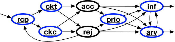
Figure 2: Directly-follows graph (DFG) of the running example.

By incorporating user-defined constraints on what properties the abstracted log shall satisfy, such a result can be avoided. For instance, if a user wants to primarily understand the interactions between employees, while abstracting from details on the individual steps performed by them, a constraint may enforce that each activity comprises only events performed by the same employee role. If applied in a naive manner, this constraint would result in two groups of events classes, i.e., $g_{\emph{clrk}}=\{\emph{rcp},\emph{ckc},\emph{ckt},\emph{prio},\emph{inf},\emph{arv}\}$ and $g_{\emph{mgr}}=\{\emph{acc},\emph{rej}\}$. Yet, using these groups directly for log abstraction is not meaningful either. The group $g_{\emph{clrk}}$ includes steps that occur at the start of the process, as well as steps that only happen at the end. Moreover, abstracting the steps in $g_{\emph{mgr}}$ to a single activity would obfuscate that $\{\emph{acc},\emph{rej}\}$ exclude each other and that only after step rej, the process is potentially restarted.

Against this background, our approach to log abstraction, gecco, aims at constructing activities for groups of events that satisfy user-specified constraints, while also preserving the behavior represented in event sequences as much as possible. For the example, this would result in an abstraction that consists of four groups: $g_{\emph{clrk1}}=\{\emph{rcp},\emph{ckc},\emph{ckt}\}$, containing the initial steps performed by the clerk, $\{\emph{acc}\}$ and $\{\emph{rej}\}$, as singleton groups of steps that are mutually exclusive and both performed by the manager, and $g_{\emph{clrk2}}=\{\emph{prio},\emph{inf},\emph{arv}\}$, the final steps of the process performed by the clerk. The directly-follows graphs obtained with this log abstraction is shown in Figure 3. It highlights that a clerk starts working on each case, before handing it over to the manager. Accepted requests are completed by the clerk, whereas rejected requests may be completed or returned to the start of the process.

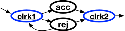
Figure 3: DFG of the log abstracted with gecco.

Obtaining the groups for such abstraction requires solving a computationally complex problem, though, as defined next.

III Problem Statement

We first define an event model for our work (§ III-A), before formalizing the addressed log-abstraction problem (§ III-B).

III-A Event model

We consider events recorded during the execution of a process and write $\mathcal{E}$ for the universe of all events. An event $e\in\mathcal{E}$ is of a certain event class, i.e., its type, which we denote as $e.C\in\mathcal{C}$, with $\mathcal{C}$ as the universe of event classes. For instance, the log in Table I consists of eight event classes, each corresponding to a specific process step. Furthermore, each event carries information about its context, which may include aspects such as a timestamp, the executing role, or relevant data values. We capture this context by a set of data attributes $\mathcal{D}=\{D_{1},\ldots,D_{p}\}$, with $dom(D_{i})$ as the domain of attribute $D_{i}$, $1\leq i\leq p$. We write $e.D$ for the value of attribute $D$ of an event $e$. For instance, in § II, each event class is assigned a particular role, i.e., a clerk or a manager. As such, an event $e$ may capture that $e.C=\emph{rcp}$ and $e.\mathit{role}=\emph{clerk}$.

A single execution of a process, called a trace, is modeled as a sequence of events $\sigma\in\mathcal{E}^{*}$, such that no event can occur in more than one trace. An event log is a set of traces, $L\subseteq 2^{\mathcal{E}^{*}}$, with $\mathcal{L}$ as the universe of all events logs, and $C_{L}\subseteq\mathcal{C}$ as the set of event classes of the events in $L$.

An event log can be represented as a directly-follows graph (DFG) that indicates if two event classes ever immediately succeed each other in the log. Given a log L, its DFG is a directed graph $(V,E)$, with the set of vertices $V$ corresponding to the event classes of $C_{L}$ and the set of edges $E\subseteq V\times V$ representing a directly-follows relation $>_{\emph{L}}$, defined as: $a>_{\emph{L}}b$, if there is a trace $\sigma=\langle e_{1},\ldots,e_{n}\rangle$ and $i\in\{1,\ldots,n-1\}$, such that $\sigma\in\emph{L}$ and $e_{i}.C=a$ and $e_{i+1}.C=b$.

III-B The log-abstraction problem

Log abstraction aims to construct groups of similar events for an event log. Formally, this is captured by a grouping, i.e., a set of groups, $\emph{G}\subset 2^{\mathcal{C}}$, over the event classes $C_{L}$, such that each class $c\in C_{L}$ is part of exactly one group $g\in\emph{G}$. Given a grouping, a function $\texttt{abstract}:\mathcal{L}\times 2^{\mathcal{C}}\rightarrow\mathcal{L}$ is applied to obtain an abstracted log $L^{\prime}$. For instance, using the log and grouping from § II, $\sigma_{1}$ is abstracted to $\sigma^{\prime}_{1}=\langle\emph{clrk1},\emph{acc},\emph{clrk2}\rangle$.

We target scenarios in which a user formulates requirements on what properties the abstracted event log and, hence, the grouping G shall satisfy, e.g., to group only events performed by a single role (see § II). Then, we aim to identify a grouping $\hat{G}$ that meets these requirements, while preserving the behavior of the traces as much as possible. To this end, we define $\texttt{dist}:\mathcal{L}\times 2^{\mathcal{C}}\rightarrow\mathbb{R}$ as a distance function that quantifies the distance of a grouping to an event log. Also, using $\mathcal{R}$ to denote the universe of possible constraints, we define a predicate $\texttt{holds}:2^{\mathcal{C}}\times\mathcal{R}\times\mathcal{L}\rightarrow\{\mathit{true},\mathit{false}\}$ to denote whether a grouping satisfies a set of constraints for a given log. Based thereon, we define the optimal log-abstraction problem:

Problem 1 (Optimal log abstraction).

Given an event log $L$ with event classes $C_{L}$, a distance function dist, and a set of constraints R, the log-abstraction problem is to find an optimal grouping $\emph{$\hat{G}$}=\{g_{1},\ldots,g_{k}\}$, such that:

• $\hat{G}$ is an exact cover of $C_{L}$, i.e., $\bigcap_{i}^{k}g_{i}=\emptyset\land\bigcup_{i}^{k}g_{i}=C_{L}$;

• $\hat{G}$ adheres to the desired constraints R, i.e., $\texttt{holds}(\emph{$\hat{G}$},\emph{R},\emph{L})=true$;

• the distance $\texttt{dist}(\emph{$\hat{G}$},\emph{L})$ is minimal.

IV gecco: Scope

To address Problem 1, we propose gecco for the Grouping of Event Classes using Constraints and Optimization. This section shows how gecco instantiates Problem 1 by specifying constraint types (§ IV-A) and a distance function (§ IV-B).

IV-A Covered constraint types

gecco is able to handle a broad range of constraints on a grouping G. As shown through the examples in § IV-A, we consider grouping constraints, class-based constraints, and instance-based constraints. The table also indicates a monotonicity property of the constraints, which is important when aiming to find an optimal grouping in an efficient manner.

TABLE II: Exemplary constraints covered by gecco.

Category	Examples	Monotonicity
Grouping constraints	There should be at most 10 groups in the final grouping.	n/a
	There should be at least 5 groups in the final grouping.	n/a
Class-based constraints	There should be at least 5 event classes per group.	monotonic
	At most 10 event classes should be grouped together.	anti-monotonic
	The event classes rcp and acc cannot be members of the same group.	anti-monotonic
	The event classes inf and arv must be members of the same group.	non-monotonic
Instance-based constraints	At least 2 distinct document codes must be associated with a group instance.	monotonic
	The cost of a group instance must be at most 500$.	anti-monotonic
	The duration of a group instance must be at most 1 hour on average.	non-monotonic
	The time between consecutive events in a group instance must at most be 10 minutes.	anti-monotonic
	Each group instance may contain at most 1 event per event class.	anti-monotonic
	At least 95% of the group instances must have a cost below 500$.	anti-monotonic

Grouping constraints. This constraint category can be used to bound the size of a grouping G, i.e., the number of high-level activities that will appear in the abstracted log. An upper bound restricts the size and complexity of the obtained log, whereas a lower bound can limit the applied degree of abstraction.

Satisfaction. We use $R_{G}\subseteq R$ to refer to the subset of grouping constraints. Whether a constraint $r\in R_{G}$ holds can be directly checked against the grouping size, $|\emph{G}|$. As such, for the holds predicate, we require $\forall r\in\emph{R}_{\emph{G}}:r(\emph{G})=\mathit{true}$.

Class-based constraints. The second category of constraints can be used to influence the characteristics of an individual group $g\in\emph{G}$ in terms of the event classes that it can contain. gecco supports any class-based constraint for which satisfaction can be checked by considering $g$ in isolation, i.e., without having to compare $g$ to other groups in G. As shown in § IV-A, this, for instance, includes constraints that each group shall comprise at least (or at most) a certain number of event classes, as well as cannot-link and must-link constraints, which may be used to specify that two event classes must or must not be grouped together.

Satisfaction. We use $R_{C}\subseteq R$ for class-based constraints. The satisfaction of a constraint $r\in R_{C}$ is directly checked by evaluating the contents of each group $g\in\emph{G}$. Hence, the holds predicate requires that $\forall g\in\emph{G},\forall r\in\emph{R}_{C}:r(g)=\mathit{true}$.

Monotonicity. Class-based constraints that specify a minimum requirement on groups, e.g., a minimal group size, are monotonic: If the constraint holds for a group $g$, it also holds for any larger group $g^{\prime}$, with $g\subset g^{\prime}$. In other words, adding event classes to a group can never result in a (new) constraint violation. By contrast, constraints that express requirements that may not be exceeded, e.g., a maximal group size or cannot-link constraint, are anti-monotonic: If they hold for a group $g$, they also hold for any subset of that group $g^{\prime}\subset g$. However, if a group $g$ violates a constraint, a larger group $g^{\prime}$, with $g\subset g^{\prime}$, also violates it.

Instance-based constraints. The third category comprises constraints that shall hold for each instance of a group $g\in\emph{G}$, i.e., a sequence of (not necessarily consecutive) events that occur in the same trace and of which the event classes are part of $g$. In line with the event context defined in § III-A, we use the shorthand $g.D$ to refer to the set of values of attribute $D$ for a group $g$ when defining constraints of this type.

As indicated in § IV-A, diverse constraints can be defined on the instance-level, relating to attribute values, associated roles, and duration, such as the total cost of an instance is at most 500$ and the average duration of group instances must be at most 1 hour. As shown in the table’s last row, also looser constraints may be expressed, such as ones that only need to hold for 95% of the respective group instances. In fact, as for class-based constraints, gecco supports all constraints of which satisfaction can be checked for an individual group $g$.

Satisfaction. We write $R_{I}\subseteq\emph{R}$ for the instance-based constraints. Contrary to the other categories, these constraints must be explicitly checked against the event log $L$, specifically for each group $g\in G$ and each instance of $g$ in the traces of $L$.

Formally, we first define a function $\texttt{inst}:\mathcal{E}^{*}\times 2^{\mathcal{C}}\rightarrow 2^{\mathcal{E}^{*}}$, which returns all instances of a group in a given trace. The operationalization of inst is straightforward for simple cases: An instance of group $g$ is the projection of the event classes of $g$ over a trace $\sigma$. In $\sigma_{1}$, $\sigma_{2}$, and $\sigma_{3}$ of our running example, exactly one instance of each group occurs per trace and, e.g., $\texttt{inst}(\sigma_{1},g_{\emph{clrk1}})=\{\langle\emph{rcp},\emph{ckc}\rangle\}$. However, processes often include recurring behavior, such as trace $\sigma_{4}=\langle$rcpwhitercp, ckcwhiteckc, rej, rcpwhitercp, cktwhiteckt, acc, priowhiteprio, infwhiteinf, arvwhitearv$\rangle$, in which a request is first rejected, sent back to the restart the process, and then accepted in the second round. Here, to detect multiple instances of a group, we instantiate function inst based on an existing technique [vanderaa2021detecting] that recognizes when a trace contains recurring behavior and splits the (projected) sequence accordingly. For the above trace, this yields $\texttt{inst}(\sigma_{4},g_{\emph{clrk1}})=\{\langle\emph{rcp},\emph{ckc}\rangle,\langle\emph{rcp},\emph{ckt}\rangle\}$. Note that inst can also be used to enforce cardinality constraints, e.g., if a user desires that each group instance should contain at least 2 events of a particular event class.

Given the function inst, a constraint $r\in R_{I}$ is satisfied if for each group $g\in\emph{G}$, $r$ holds for each instance $\xi\in\texttt{inst}(\sigma,g)$, for each $\sigma\in L$. Note that constraints are vacuously satisfied for traces that do not include an instance of a particular group, i.e., where $\texttt{inst}(\sigma,g)=\emptyset$. Therefore, for instance-based constraints, holds is checked for each $g\in\emph{G}$ as $\forall\ r\in\emph{R}_{I},\forall\ \sigma_{i}\in\emph{L},\forall\ \xi\in\texttt{inst}(\sigma_{i},g):r(\xi)=\mathit{true}$. For looser constraints, e.g., ones that should for 95% of the group instances, predicate satisfaction is adapted accordingly.

Monotonicity. As is the case for class-based ones, instance-based constraints are monotonic when they specify a minimum requirement to be met, e.g., each instance should take at least one hour, and anti-monotonic when they specify something that may not be exceeded, e.g., each instance may take at most one hour. However, constraints in $R_{I}$ may also be based on aggregations that behave in a non-monotonic manner, such as constraints that consider the average or variance of attribute values per group instance or sums including negative values. In these cases, adding and removing event classes from a group can result in a violated constraint to now hold or vice versa.

IV-B Distance measure

To determine which event classes are suitable candidates to be grouped together, we employ a distance function $\texttt{dist}(\emph{G},\emph{L})$ that quantifies the relatedness of the event classes per group. Although our work is largely independent of a specific distance function, we argue that log abstraction should group together event classes such that 1. events within a group are cohesive, i.e., the events belonging to a single group instance occur close to each other, meaning there are few interspersed events from other instances; 2. events within a group are correlated, i.e., the events belonging to a single group typically occur together in the same trace and group instance; 3. larger groups are favored over unary groups, i.e., the grouping G actually results in an abstraction. To capture these three aspects, we propose the following distance function for an individual group $g$ and a log $L$:

$$\texttt{dist}(g,L)=\sum\limits_{\xi\in\texttt{inst}(L,g)}\frac{\frac{\texttt{interrupts}(\xi)}{|\xi|}+\frac{\texttt{missing}(\xi,g)}{|g|}+\frac{1}{|g|}}{|\texttt{inst}(L,g)|}$$ (1)

The first summand in the numerator of Eq. 1 considers cohesion. Here, $\texttt{interrupts}(\xi)$ counts how many events from other instances are interspersed between the first and last events of a given group instance $\xi$. As such, this penalizes groups of events that are often interrupted by others, e.g., in a trace $\langle a,b,c,d,e\rangle$, grouping $a$ and $e$ together is unfavorable, since the instance $\langle a,e\rangle$ has three interspersed events. In Eq. 1, the number of interruptions is considered relative to the length of $\xi$. The second summand in the numerator of Eq. 1 quantifies the degree of completeness of $\xi$ with respect to $g$, thus capturing the correlation between the events in $g$. Here, $\texttt{missing}(\xi,g)$ returns how many event classes from $g$ are missing from its instance $\xi$, which is then offset against the total number of classes $|g|$. Finally, since groups with a single event class have perfect cohesion and correlation by default, we include $\frac{1}{|g|}$ to ensure that larger groups with the same cohesion and correlation are favored, thus avoiding unary groups when possible.

Finally, to quantify the entire distance of a grouping $G$, we sum up the distance values of all groups in $G$, resulting in the following function that will be minimized in our approach:

$$\texttt{dist}(\emph{G},\emph{L})=\sum_{g\in\emph{G}}\texttt{dist}(g,\emph{L})$$ (2)

V The gecco Approach

Next, we describe how gecco achieves the goal of finding an optimal event grouping, given the distance function and constraints defined above. § V-A provides a high-level overview, while § V-B to § V-D outline the algorithmic details.

V-A Approach Overview

As shown in Figure 4, gecco takes an event log L and a set of user-defined constraints R as input. Then, gecco applies three main steps in order to obtain an abstracted log $L^{\prime}$.

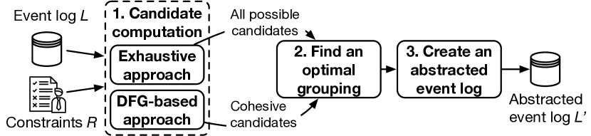
Figure 4: The main steps of gecco.

In Step 1, gecco computes a set of candidate groups $\mathcal{G}$, i.e., groups of event classes that adhere to the constraints in R. As depicted in Figure 4, we propose two instantiations for this step: an exhaustive instantiation and an efficient DFG-based one. The exhaustive instantiation yields a set of candidates that is guaranteed to be complete and, thus, assures that it can afterwards be used to establish an optimal grouping if it exists.

However, this approach may be intractable in practice. Therefore, we also propose a DFG-based alternative, which only retrieves cohesive candidates, i.e., candidates likely to be part of an optimal grouping. By exploiting the process-oriented nature of the input data, cohesive candidates are identified efficiently. Any solution obtained using this instantiation is still guaranteed to satisfy the constraints in R, yet may have a sub-optimal distance score.

In Step 2, gecco uses the identified set of candidates in order to find a single optimal grouping G that minimizes the distance function dist, while ensuring that all constraints are met and each event class in $C_{L}$ is assigned to exactly one group in G. To achieve this, we formulate this task as a mixed-integer programming (MIP) problem.

Finally, having obtained a grouping G, Step 3 abstracts event log L by replacing the events in a trace with activities based on groups defined in G, yielding an abstracted log L’.

V-B Step 1: Computation of candidate groups

In this step, gecco computes a set of candidate groups of event classes, $\mathcal{G}$, i.e., subsets of $C_{L}$ that adhere to constraints in R. As described in § V-A, we propose an exhaustive and a DFG-based instantiation for this step:

Exhaustive candidate computation. To obtain a complete set of candidate groups, in principle, every combination of event classes, i.e., every subset of $C_{L}$, needs to be checked against the constraints in R. However, we are able to considerably reduce this search space by (for the moment) only looking for groups $g\subseteq C_{L}$ that actually co-occur in at least one trace in the log (referred to as group co-occurrence) and by considering the monotonicity of the constraints in R. Then, candidate groups of increasing size can be identified iteratively, as outlined in § V-B.

Algorithm 1 Exhaustive candidate computation

t Input Event log L, user constraints R

t Output Set of candidate groups $\mathcal{G}$

1:mode $\leftarrow$ setCheckingMode(R)

2:toCheck $\leftarrow\{\ \{c\}$ for $c\in C_{L}\}$ $\triangleright$ Set the first groups to check

3:while toCheck $\neq\emptyset$  do

4:    if mode = monotonic then

5:         $\mathcal{G}_{new}\leftarrow\{g\in$ toCheck if $\exists g^{\prime}\in\mathcal{G}:g^{\prime}\subset g$
xxxxxxxxxxxxxxxxxxxxxxxxx $\lor\ \texttt{holds}(g,\emph{L},\emph{R})$

6:    else

7:         $\mathcal{G}_{new}\leftarrow\{g\in$ toCheck if $\texttt{holds}(g,\emph{L},\emph{R})\}$     

8:    $\mathcal{G}\leftarrow\mathcal{G}~{}\cup\mathcal{G}_{new}$

9:    if mode = anti-monotonic then

10:         toCheck $\leftarrow$ expandGroups($\mathcal{G}_{new}$)

11:    else

12:         toCheck $\leftarrow$ expandGroups(toCheck)     

13:    toCheck $\leftarrow\{g\in$ toCheck if $\texttt{occurs}(g,L)\}$

14:return $\mathcal{G}$

Initialization. We first set the constraint-checking mode that shall be applied (line 1) based on the monotonicity of the constraints in R. Specifically, mode is set to anti-monotonic if R contains at least one such constraint, to monotonic if all constraints in $\emph{R}\setminus\emph{R}_{G}$ are monotonic (i.e., all constraints that must be checked per group), and otherwise to non-monotonic.

Using this constraint-checking mode, we employ two pruning strategies. First, consider a group $g_{1}\subset C_{L}$ and a constraint set R in which all constraints $\emph{R}\setminus\emph{R}_{G}$ are monotonic. If $\texttt{holds}(g_{1},\emph{R},L)=\mathit{true}$, any supergroup $g^{\prime}_{1}\supseteq g_{1}$ will also adhere to the constraints, since adding more event classes to $g_{1}$ will never lead to a violation of a monotonic constraint. Therefore, in the monotonic mode, we can avoid the costs of constraint validation for $g^{\prime}_{1}$. Second, consider a group $g_{2}\subset C_{L}$, known to violate any anti-monotonic constraint in R, i.e, $\texttt{holds}(g_{2},\emph{R},L)=\mathit{false}$. Then we also know that no supergroup $g^{\prime}_{2}\supseteq g_{2}$ can adhere to R, as expanding a group can never resolve violations of anti-monotonic constraints. Thus, in the anti-monotonic mode, all supergroups of $g_{2}$ can be skipped.

With mode set, the algorithm then adds all event classes of $C_{L}$ as singleton groups to the set of potential candidates, toCheck, which shall be checked in the first iteration (line 2).

Candidate assessment. In each iteration, § V-B first establishes a set $\mathcal{G}_{new}$, which contains all groups in toCheck that adhere to the constraints in R. When validating a group, we check constraints in $\emph{R}_{C}$ before ones in $\emph{R}_{I}$, since the former do not require a pass over the event log, thus, minimizing the validation cost per candidate. In the monotonic mode, the algorithm employs the first pruning strategy by directly adding any group $g$, for which there is a $g^{\prime}\subset g$ already in $\mathcal{G}$, given that we then know that the monotonic constraints will be satisfied for $g$ as well (line 5). For other groups and for the other two modes, we need to check $\texttt{holds}(g,L,R)$ for each group $g\in\mathit{toCheck}$ (lines 5 and 7). Having established $\mathcal{G}_{new}$, the new candidates are added to the total set $\mathcal{G}$ (line 8).

Group expansion. Next, the algorithm repopulates toCheck with larger groups that shall be assessed in the next iteration. In the anti-monotonic mode, using the second pruning strategy, the algorithm only needs to expand groups that are known to adhere to all anti-monotonic constraints in $R$. Therefore, in this case, we only expand the groups in $\mathcal{G}_{new}$ (line 10). This expansion involves the creation of new groups that consist of a group $g\in\mathcal{G}_{new}$ with an additional event class from $C_{L}$. Naturally, the anti-monotonic mode avoids the creation of groups that contain subgroups that are already known to violate R. For the monotonic and non-monotonic mode, we also need to expand groups that currently violate the constraints, since their supergroups may still lead to constraint satisfaction. Therefore, these modes expand all groups in toCheck (line 12). Afterwards, we only retain those groups in toCheck$(g,L)$ that actually occur in the event log, by checking if there is at least one trace in $L$ that contains events corresponding to all event classes in $g$ (line 13).

Termination. The algorithm stops if there are no new candidates to be checked, returning the set of all candidates, $\mathcal{G}$.

Computational complexity. While § V-B is guaranteed to yield a complete set of candidates, its time complexity is exponential with respect to the number of event classes in the event log, i.e., $2^{|C_{L}|}$. In the worst case, each of the subsets of $C_{L}$ must be analyzed against the entire log, where primarily the number of traces is important, since each group must be separately checked against all traces. Given that each checked group may become a candidate, the algorithm’s space complexity is also bounded by $2^{|C_{L}|}$. Hence, this exhaustive approach can quickly become infeasible.

DFG-based candidate computation. In the light of the runtime complexity of the exhaustive approach, we also propose a DFG-based approach to compute candidate groups. It exploits behavioral regularities in event logs in order to efficiently derive a set of cohesive candidate groups.

Intuition. Log abstraction aims to find cohesive groups of event classes and, therefore, is more likely to group together event classes that occur close to each other. In our running example, even though the request receipt (rcp) and archive request (arv) event classes meet the constraint (both are performed by a clerk), it is unlikely that they will end up in the same activity in an optimal grouping $G$, since rcp occurs at the start of each trace and arv at the end.

We exploit this characteristic of optimal groupings by identifying only candidates that occur near each other. This is achieved by establishing a DFG of the event log and traversing this graph to find highly cohesive candidates groups. Since this traversal again iteratively increases the candidate size, we can still apply the aforementioned pruning strategies.

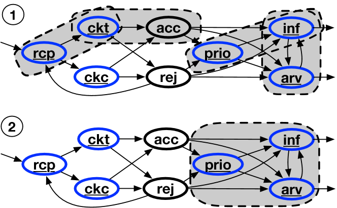
Figure 5: DFG-based candidate computation (Iterations 1 & 2).

This idea is illustrated in Figure 5, which visualizes (parts of) two iterations for the running example, highlighting candidate groups that are checked. Iteration 1 involves the assessment of paths of length two, consisting of connected event classes. This identifies, e.g., the candidate paths [prio,inf], [prio,arv], and [inf,arv], which all adhere to the constraint, whereas, e.g., [acc, inf] is recognized as a violating path, since acc and inf are performed by different roles. Given their distance from each other in the DFG, this iteration avoids checking groups such as {rcp, arv} and {ckt, inf}. In the next iteration, since the running example deals with an anti-monotonic constraint, we concatenate pairs of constraint-adhering paths to obtain candidate paths (i.e., groups) of length three, as shown for [prio, inf, arv] in Figure 5.

The DFG-based approach works as described in § V-B. Next to an event log $L$ and a constraint set R, it takes as input a parameter $k$, defining the beam-search width.

Initialization. The algorithm starts by again setting the constraint-checking mode (line 1), before establishing the log’s DFG (line 2), as defined in § III-A. Then, for every node $n$ in the DFG (i.e., for every event class), we add the trivial path $\langle n\rangle$ to the set of candidates to check in the first iteration (line 3).

Algorithm 2 DFG-based candidate computation

t Input event log L, user constraints R, pruning parameter $k$

t Output Set of candidate groups $\mathcal{G}$

1:mode $\leftarrow$ setCheckingMode(R)

2:$\mathit{DFG}\leftarrow$ computeDFG($L$)

3:toCheck $\leftarrow\{\langle n\rangle$ for $n\in\mathit{DFG}.\texttt{nodes}\}$ $\triangleright$ First paths to check

4:while toCheck $\neq\emptyset$ do

5:    sortedPaths $\leftarrow\texttt{sort}(\textit{toCheck},\texttt{dist})$ $\triangleright$ Lowest dist first

6:    $\emph{toExpand}\leftarrow\emptyset$

7:    $i\leftarrow 0$

8:    while $i<\min(|\emph{sortedPaths}|,k)$ do

9:         $p\leftarrow\emph{sortedPaths}[i]$ $\triangleright$ Get next path

10:         $g\leftarrow\texttt{nodes}(p)$ $\triangleright$ Derive nodes, i.e., event classes of $p$

11:         if mode = monotonic then

12:             if $\exists g^{\prime}\in\mathcal{G}:g^{\prime}\subset g\lor\ \texttt{holds}(g,\emph{L},\emph{R})$  then

13:                 $\mathcal{G}\leftarrow\mathcal{G}\cup\{g\}$              

14:             $toExpand\leftarrow toExpand\cup\{p\}$

15:         else if $\texttt{holds}(g,L,R)$  then

16:             $\mathcal{G}\leftarrow\mathcal{G}\cup\{g\}$

17:             $toExpand\leftarrow toExpand\cup\{p\}$

18:         else if $mode\neq$ anti-monotonic then

19:             $toExpand\leftarrow toExpand\cup\{p\}$          

20:         $i\leftarrow i+1$     

21:    toCheck $\leftarrow\emptyset$ $\triangleright$ Start computing new paths to check

22:    for $p=\langle p_{0},\ldots,p_{m}\rangle\in\emph{toExpand}$  do

23:         for $(p_{m},\emph{succ})\in\mathit{DFG}.\texttt{outgoingEdges}(p_{m})$  do

24:             if $\emph{succ}\notin\texttt{nodes}(p)$ then

25:                 $\emph{toCheck}\leftarrow\emph{toCheck}\cup\{\ \langle p_{0},\ldots,p_{m},\emph{succ}\rangle~{}\}$                       

26:         for $(\emph{pred},p_{0})\in\mathit{DFG}.\texttt{incomingEdges}(p_{0})$  do

27:             if $\emph{pred}\notin\texttt{nodes}(p)$ then

28:                 $\emph{toCheck}\leftarrow\emph{toCheck}\cup\{\ \langle\emph{pred},p_{0},\ldots,p_{m}\rangle~{}\}$                           

29:    toCheck $\leftarrow\{p\in$ toCheck if $\texttt{occurs}(\texttt{nodes}(p),\emph{L})\}$

30:return $\mathcal{G}$

Candidate assessment. In principle we could assess for each path $p\in\emph{toCheck}$ if $p$’s nodes form a proper candidate group, as we do in the exhaustive approach. However, we here recognize that in event logs with a lot of variability, the number of paths to check will still be considerable. Hence, we allow for a further pruning of the search space by incorporating a beam-search [Wilt2010] component in the algorithm. In this beam search, we only keep the $k$ most promising candidates (i.e., the beam) in each iteration of the algorithm.

To do this, each iteration starts by sorting the candidate paths in toCheck, giving priority to paths of which the nodes have the lowest distance to each other, according to $\texttt{dist}(\texttt{nodes(p)},L)$ (line 5). Then, the algorithm picks candidates from sortedPaths as long as there are candidates to pick and the beam width $k$ has not been reached (line 8). Each group $g$, defined by the nodes in a path (i.e., $g=\texttt{nodes}(p)$), is then checked for constraint satisfaction. As for the exhaustive approach, we check constraints in $\emph{R}_{C}$ before ones in $\emph{R}_{I}$ minimizing validation cost per candidate.

Here, we employ the same pruning strategies for monotonic and anti-monotonic constraint-checking modes as done for the exhaustive approach. Therefore, in the monotonic mode, a group $g$ can be directly added to the set of candidates $\mathcal{G}$ if we have already seen a subset $g^{\prime}\subset g$ that adheres to the constraints (lines 12–13), whereas in the anti-monotonic mode, we no longer expand paths that violate the constraints (lines 18–19).

Path expansion. The candidates for the next iteration are created by expanding paths in toExpand with either a predecessor of their first or a successor of their last node (lines 22–28). Again, we then only retain those paths in toCheck, whose groups $g$ actually occur in the event log (line 29).

Termination. The algorithm stops if no candidates are left, i.e., toCheck is empty and the set $\mathcal{G}$ is returned.

Computational complexity. The DFG-based approach is considerably more efficient than the exhaustive one. In each iteration, the approach expands up to $k$ groups, each into up to $|C_{L}|-1$ new candidates. As such, given the maximum of $|C_{L}|$ iterations, the worst-case time and space complexity is $k*|C_{L}|^{2}$. Moreover, this worst case only occurs if the DFG is a complete digraph and no constraints are imposed.

Dealing with exclusion. Generally, it is undesirable to group exclusive event classes together, since such classes never occur in the same trace. This is why we have so far omitted these from consideration, by ensuring that occurs$(g,L)$ holds for every candidate group $g\in\mathcal{G}$. Yet, when exclusive event classes (or groups) are proper alternatives to each other, we make an exception for this. In these cases, grouping them together will result in a further complexity reduction of the event log, while not affecting its expressiveness.

Intuition. To illustrate this, reconsider the running example, which contains two sets of exclusive event classes, {ckc, ckt}, corresponding to two ways in which a request can be checked, and {acc, rej}, corresponding to acceptance and rejection of a request. By considering Figure 6, we see that the former two event classes are proper behavioral alternatives: both ckc and ckt are preceded and followed by the exact same sets of event classes.As such, behavioral alternatives can be defined as groups of event classes that have identical pre- and postsets in the DFG. Merging them will thus not lead to a loss of behavioral information. By contrast, acc and rej do not represent proper alternatives to each other, since their postsets differ. Particularly, while after acceptance the process always moves forward to one of the event classes in {prio, inf, arv}, a rejection may also result in a loop back to the start of the process (rcp). Therefore, if these exclusive classes were merged, we would obscure the fact that there are two different possibilities here.

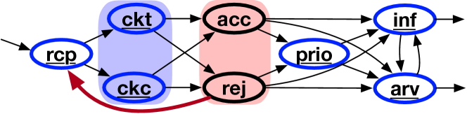
Figure 6: DFG of the running example highlighting proper behavioral alternatives (blue) and exclusive event classes, which are no behavioral alternatives (red).

Candidate identification. We employ § V-B to determine if previously identified candidate groups in $\mathcal{G}$, with excluding event classes, can be merged to obtain additional candidates.

The algorithm establishes a set equivGroups consisting of candidate groups that share the same pre- and postset (line 4). Then, a stack is created consisting of all pairs of groups in this set (lines 5–7). For each pair $(g_{i},g_{j})$ in this stack, we assess if $g_{i}$ and $g_{j}$ are indeed exclusive to each other and if their merged group, $g_{ij}$, still adheres to the user constraints (line 11). Both conditions can be efficiently checked. The former by ensuring that there are no edges from nodes in $g_{i}$ to nodes in $g_{j}$ or vice versa, while for the latter only adherence to class-based constraints ($R_{C}$) needs to be assessed, given that instance-based constraints cannot be (newly) violated when merging exclusive groups, thus avoiding a pass over the event log $L$.

If $g_{ij}$ is indeed a proper, new candidate, we next determine if this group can also be combined together with its preset, postset, or with both, to create more candidates (lines 13–19). For instance, having identified {ckt, ckc} as a new candidate group for the running example, we would this way recognize that this new group together with its preset (event class rcp) also forms a proper candidate group: {rcp, ckt, ckc}, since both {rcp, ckt} and {rcp, ckc} were also already part of $\mathcal{G}$.

After establishing these new candidates, the algorithm adds any new pair $(g_{ij},g_{k})$ to the stack, so that also iteratively larger candidates, consisting of three or more exclusive groups, can be identified (lines 20–21). The algorithm terminates when all relevant pairs have been assessed, returning the updated set $\mathcal{G}$ as the final output of Step 1 of the approach.

Algorithm 3 Find exclusive candidate groups

t Input Event log L, user constraints R, current candidate groups

t Output Extended set of candidate groups $\mathcal{G}$

1:$\mathit{DFG}\leftarrow$ computeDFG($L$)

2:$\emph{seenGroups}\leftarrow\emptyset$

3:for $g\in\mathcal{G}\setminus\emph{seenGroups}$ do

4:    equivGroups $\leftarrow\mathit{DFG}$.equalPrePost($g$) $\cup\ \{g\}$

5:    pairsToCheck $\leftarrow\texttt{new Stack}()$

6:    for $(g_{i},g_{j})\in\emph{equivGroups}\times\emph{equivGroups}$ do

7:         pairsToCheck.push$\left((g_{i},g_{j})\right)$     

8:    while $\neg\emph{pairsToCheck}.\texttt{isEmpty}()$ do

9:         $(g_{i},g_{j})\leftarrow\emph{pairsToCheck}.\texttt{pop}()$

10:         $g_{ij}\leftarrow g_{i}\cup g_{j}$ $\triangleright$ Merge into single group

11:         if exclusive($g_{i},g_{j})\land\texttt{holds}(g_{ij},L,R_{C})$ then

12:             $\mathcal{G}\leftarrow\mathcal{G}\cup\{g_{ij}\}$ $\triangleright$ New candidate found

13:             (pre, post) $\leftarrow(\mathit{DFG}$.pre($g_{i}$), $\mathit{DFG}$.post($g_{i}$))

14:             if pre $\cup$ post $\cup\ g_{i}\in\mathcal{G}~{}\land$ pre $\cup$ post $\cup\ g_{j}\in\mathcal{G}$ then

15:                 $\mathcal{G}\leftarrow\mathcal{G}\cup\{\emph{pre}\cup\emph{post}\cup g_{ij}\}$

16:             else if pre $\cup\ g_{i}\in\mathcal{G}~{}\land$ pre $\cup\ g_{j}\in\mathcal{G}$ then

17:                 $\mathcal{G}\leftarrow\mathcal{G}\cup\{$pre $\cup~{}g_{ij}\}$

18:             else if post $\cup~{}g_{i}\in\mathcal{G}~{}\land~{}$post $\cup~{}g_{j}\in\mathcal{G}$ then

19:                 $\mathcal{G}\leftarrow\mathcal{G}\cup\{$post $\cup~{}g_{ij}\}$              

20:             for $g_{k}\in\emph{equivGroups}\setminus\{g_{i},g_{j}\}$  do

21:                 pairsToCheck.push$\left((g_{ij},g_{k})\right)$              

22:             equivGroups $\leftarrow\emph{equivGroups}\cup\{g_{ij}\}$              

23:    seenGroups $\leftarrow\emph{seenGroups}\cup\emph{equivGroups}$

24:return $\mathcal{G}$

Computational complexity. § V-B has linear complexity with respect to $|\mathcal{G}|$, i.e., the number of candidate groups stemming from the previous step. As such, its worst-case time and space complexity is $2^{|C_{L}|}$ when previously using the exhaustive approach and $k*|C_{L}|^{2}$ for the DFG-based one.

V-C Step 2: Finding an optimal grouping

Having established candidate groups $\mathcal{G}$, we set out to find an optimal grouping $\emph{G}\subseteq\mathcal{G}$ based on these candidates, which is a set of disjoint groups that covers all event classes, while minimizing the overall distance. We formulate this task as a MIP problem, which can be tackled using standard solvers.

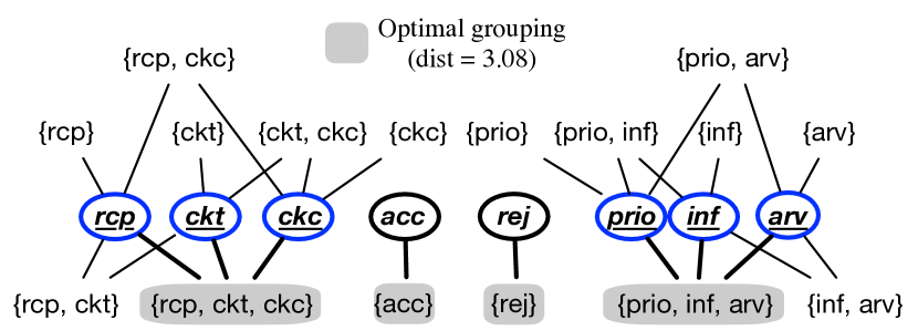
Figure 7: Optimal grouping of the running example given all candidates computed in step 1 using the DFG-based approach.

Central to this formulation is a bipartite graph $(\mathcal{G},C_{L},E)$, which connects each candidate group to the event classes it covers, i.e., it contains an edge $(g_{i},c_{j})\in E$ if $c_{j}\in g_{i}$. Figure 7 visualizes this for the running example, in which the circled nodes in the middle indicate event classes in $C_{L}$, the sets indicate the candidate groups $\mathcal{G}$, and the edges their coverage relation. The grayed sets highlight the optimal grouping in this case, which is an exact cover because every event-class node is connected to exactly one of the selected groups.

Given this bipartite graph $(\mathcal{G},C_{L},E)$, we formalize a MIP problem with two decision variables:

• $selected_{g_{i}}\in\{0,1\}$: 1 if $g_{i}\in\mathcal{G}$ is selected, else 0;

• $covered_{c_{j}}\in\{0,1\}$: 1 if $c_{j}\in C_{L}$ is covered, else 0.

Then, we seek to minimize the distance of the selected groups in the objective function:

$$\text{minimize}\ \displaystyle\sum\limits_{g_{i}\in\mathcal{G}}\texttt{dist}(g_{i})*selected_{g_{i}}$$

This objective function is subject to two constraints:

$$\sum\limits_{j=1}^{|C_{L}|}covered_{c_{j}}=|C_{L}|$$ (3)

$$\sum\limits_{(g_{i},c_{j})\in E}selected_{g_{i}}=covered_{c_{j}},\forall c_{j}\in C_{L}$$ (4)

These constraints jointly express that each event class shall be covered (Eq. 3), by exactly one group (Eq. 4). In case a user imposes grouping constraints in $R_{G}$, bounding the number of groups that may be selected, these are imposed by adding either or both of the following additional constraints:

$$\begin{array}[]{ll@{}ll}\displaystyle\sum\limits_{i=1}^{|\mathcal{G}|}~{}selected_{g_{i}}\leq x&\text{resp.}&&\displaystyle\sum\limits_{i=1}^{|\mathcal{G}|}~{}selected_{g_{i}}\geq y\end{array}$$ (5)

The selected groups, i.e., $\emph{G}=\{g_{i}\in\mathcal{G}:\emph{selected}_{g_{i}}=1\}$, then form the obtained grouping.

Note that, depending on the characteristics of log $L$ and the imposed constraints $R$, a grouping may not be found, since there is no guarantee that a feasible solution exists. In that case, gecco returns the initial log. To allow users to then refine their constraints appropriately, gecco also indicates possible causes of the infeasibility, e.g., the affected event classes that lead to violations for constraints in $\emph{R}_{C}$, or the fraction of cases for which constraints in $\emph{R}_{I}$ are violated. If a solution is found, gecco continues with its third and final step.

Computational complexity. Most MIP problems are NP-hard, although an assessment of the exact complexity depends on the concrete problem and is poorly characterized by input size [mipcomplexity]. However, solvers like Gurobi are often able to solve MIP problems efficiently, by applying pre-solvers and heuristics. Our experiments confirm this, showing that Step 2 only contributes marginally to the overall runtime of gecco.

V-D Step 3: Creating an abstracted event log

Finally, we use the grouping G to establish abstracted versions of the traces in $L$ to obtain an abstracted log $L^{\prime}$.

For each trace $\sigma\in L$, we identify all activity instances in the trace, i.e., all instances of groups in G, $\mathcal{I}^{\sigma}=\bigcup_{g\in\emph{G}}\texttt{inst}(\sigma,g)$. Each activity instance, $\xi_{i}\in\mathcal{I}^{\sigma}$, corresponds to an ordered sequence of events, $\langle e_{1},...,e_{k}\rangle$.

Next, our approach creates an abstracted trace $\sigma^{\prime}$, which reflects the activity instances in $\mathcal{I}^{\sigma}$, instead of the events of its original counterpart, $\sigma$. A common abstraction strategy is to let $\sigma^{\prime}$ capture only the completion of activity instances, by creating a projection of $\sigma$ that only retains the last event, $e_{k}$, per activity instance. For instance, for trace $\sigma_{1}=\langle$rcpwhitercp, ckcwhiteckc, acc, priowhiteprio, infwhiteinf, arvwhitearv$\rangle$ of the running example, this abstraction would yield $\sigma^{c}_{1}=\langle$clrk1whiteclrk1, acc, clrk2whiteclrk2$\rangle$.

Yet, this strategy may obscure information when activities are executed in an interleaving manner. For this, consider a new trace $\sigma_{5}=\langle$rcpwhitercp, ckcwhiteckc, priowhiteprio, acc, infwhiteinf, arvwhitearv$\rangle$. Here, events belonging to the clrk2 group occur both before (prio) and after (inf, arv) the unary activity instance acc. When only retaining completion events, this yields the trace $\sigma^{c}_{5^{\prime}}=\langle$clrk1whiteclrk1, acc, clrk2whiteclrk2$\rangle$, which hides the interleaving nature of the activities.

Therefore, we also propose an alternative strategy, which retains both the start (s) and completion (c) events per activity instance $\xi_{i}\in\mathcal{I}^{\sigma}$. This yields a trace $\sigma^{s+c}_{5^{\prime}}=\langle{\color[rgb]{0,0,1}\underline{\emph{clrk1}_{s}}},{\color[rgb]{0,0,1}\underline{\emph{clrk1}_{c}}}$, ${\color[rgb]{.25,.25,.25}\underline{\emph{clrk2}_{s}}}$, acc, ${\color[rgb]{.25,.25,.25}\underline{\emph{clrk2}_{c}}}\rangle$, which thus shows that activity clrk2 starts before acc and completes afterwards.

The choice for a particular strategy depends on the relevance of parallelism in a particular analysis context, given that the latter strategy also leads to longer traces, thus partially mitigating the benefits of the obtained log abstraction.

The log $L^{\prime}$ that results from this last step represents the final output of gecco. It is an event log in which the high-level activities are guaranteed to satisfy the user-defined constraints in R while providing a maximal degree of abstraction.

VI Experimental Evaluation

We evaluated gecco through evaluation experiments using a collection of real-world event logs. § VI-A outlines the evaluation setup. § VI-B reports on the results obtained for our approach and its configurations, whereas § VI-C compares our work against three baselines. Finally, § VI-D further illustrates the value of constraint-driven log abstraction through a case study. The employed implementation, evaluation pipelines, and additional experimental results are all publicly available.

VI-A Evaluation Setup

Implementation and environment. We implemented our approach in Python, using PM4Py [pm4py] for event log handling and Gurobi [gurobi] as a solver for MIP problems. All experiments were conducted single-threaded on an Intel Xeon 2.6 GHz processor with up to 768GB of RAM available.

Data collection. We use a collection of 13 publicly-available event logs. To be able to cover various constraints, all logs have at least one categorical event attribute, as well as timestamps used for numerical constraints. As shown in Table III, the logs vary considerably in terms of key characteristics, such as the number of event classes, traces, and variants.

TABLE III: Properties of the real-life log collection.

Ref	$\mathbf{|C_{L}|}$	Traces	Variants	$\mathbf{|E|}$	Avg $\mathbf{|\sigma|}$
[rtfm]	11	150,370	231	70	3.73
[bpi2019]	40	75,928	3,453	357	6.35
[bpi2014]	39	46,616	22,632	772	10.01
[bpi2017]	24	31,509	5,946	180	16.41
[bpic2018]	39	14,550	8,627	407	52.48
[bpi2012]	24	13,087	4,366	125	20.04
[credit]	8	10,035	1	14	15.00
[bpi2020]	51	7,065	1,478	553	12.25
[bpi2013]	4	1,487	183	10	4.47
[wabo]	27	1,434	116	99	5.98
[sepsis]	16	1,050	846	115	14.49
[bpi151]	70	902	295	124	24.00
[ccc2019]	29	20	20	164	69.70

Constraints. We use ten constraint sets in our experiments, covering the various constraint types that gecco supports. Each set includes the class-based constraint $|g|\leq 8$, which is used to limit the number of abstraction problems that time out. This constraint is combined with each of the sets from Table IV, covering anti-monotonic ($A$), monotonic ($M$), and non-monotonic ($N$) instance-based constraints, a grouping constraint (Gr), as well as two sets of their combinations ($C1$ and $C2$). Table IV also contains additional constraints ($BL1$ to $BL4$) used in baseline comparisons, described below. By combining these constraint sets with the 13 event logs, we establish a total of 121 abstraction problems to be solved.

TABLE IV: Constraints used in the experiments.

ID	Categories	Constraint(s)
$A$	$\emph{R}_{I}$	$|g.role|\leq 3$
$M$	$\emph{R}_{I}$	$\texttt{sum}(g.duration)\geq 10^{1}$
$N$	$\emph{R}_{I}$	$\texttt{avg}(g.duration)\leq 5*10^{5}$
$Gr$	$\emph{R}_{G}$	$|G|\leq 3$
$C1$	$\emph{R}_{I},\emph{R}_{G}$	$A\land N\land Gr$
$C2$	$\emph{R}_{I},\emph{R}_{G}$	$A\land M\land N\land Gr$
$BL1$	$\emph{R}_{C}$	$|g|\leq 5$
$BL2$	$\emph{R}_{C}$	$BL1$ $\land$ cannotLink($e_{1}.C,e_{2}.C$)
$BL3$	$\emph{R}_{C}$	$|g.D|=1$
$BL4$	$\emph{R}_{G}$	$|G|=\nicefrac{{|L|}}{{2}}$

Configurations. We test three configurations that differ in the instantiation of Step 1 of gecco (cf., § V-B):

• exh, using exhaustive candidate computation;

• dfg${}_{\infty}$, using the DFG-based instantiation without beam search (i.e., unlimited beam width);

• dfg${}_{k}$, using the DFG-based instantiation with a beam width that adapts to the number of event classes in the given log, i.e., $k$ = $5*|C_{L}|$.

Note that we let candidate computation time out after 5 hours. gecco then continues with the candidates identified so far.

Baselines. We compare gecco against three baselines. These represent alternative approaches to solve the log-abstraction problem and differ in the scope of constraints they can handle.

Graph querying (bl${}_{\mathit{Q}}$). gecco’s DFG-based candidate computation traverses a DFG to find candidate groups that adhere to imposed constraints. Recognizing the overlap of this with graph querying, bl${}_{\mathit{Q}}$ replaces replaces Step 1 of gecco with an instantiation using graph querying. For this, the DFG is stored in a graph database, which is queried for candidate groups using constraints formulated in a state-of-the-art graph querying language [cypher18]. Given that a DFG captures a log on the class-level, bl${}_{\mathit{Q}}$ can only support class-based constraints, though. Thus, we assess bl${}_{\mathit{Q}}$ using a constraint on the maximum group size ($BL1$), an additional cannot-link constraint between event classes ($BL2$), and a constraint over a class-level attribute ($BL3$). By comparing against bl${}_{\mathit{Q}}$, we aim to show that gecco yields more comprehensive sets of candidate groups than those obtained by adopting existing solutions.

Graph partitioning (bl${}_{\mathit{P}}$). gecco’s goal to find a disjoint set of cohesive groups for log abstraction is similar to the goal of graph partitioning, which aims to partition a graph such that edges between different groups have a low weight [luxburg2007spectral]. Therefore, we compare gecco against a baseline using such partitioning, bl${}_{\mathit{P}}$. Given a DFG, bl${}_{\mathit{P}}$ aims to minimize the sum of directly-follows frequencies of cut edges, while cutting the graph into $n$ partitions. For this, bl${}_{\mathit{P}}$ applies spectral partitioning [luxburg2007spectral], where the weighted adjacency matrix is populated using normalized directly-follows frequencies. Since graph partitioning simply splits a DFG into a certain number of groups, bl${}_{\mathit{P}}$ can only support strict grouping constraints, whereas instance-based, class-based, and flexible grouping constraints (e.g., constraint $Gr$), cannot be handled. Therefore, we compare bl${}_{\mathit{P}}$ against gecco using the constraint $BL4$, which aims to reduce number of event classes of a log by half. This comparison aims to show that gecco’s three-step approach leads to better log-abstraction results, while also supporting a considerably broader range of constraints.

Greedy approach (bl${}_{G}$). Finally, we compare gecco against a greedy abstraction strategy. bl${}_{G}$ starts by assigning all event classes from $C_{L}$ to a set of singleton groups, $G_{0}$. Then, in each iteration, bl${}_{G}$ merges those two groups from $G_{i}$ that lead to the lowest overall distance, i.e., $\texttt{dist}(G_{i+1},L)$, without resulting in any constraint violations. bl${}_{G}$ stops if the overall distance cannot improve in an iteration. Unlike the other baselines, bl${}_{G}$ can handle instance-based constraints, since it works directly on the event log rather than the DFG, although, grouping constraints cannot be enforced in this iterative strategy. Therefore, we compare bl${}_{G}$ against gecco using the instance-based constraint set $A$, $M$, and $N$. This comparison against bl${}_{G}$ aims to show the importance of striving for a global optimum in the log-abstraction problem.

Measures. To assess the results obtained by the various configurations and baselines, we consider the following measures:

Solved abstraction problems (Solved).: We report on the fraction of solved problems, to reflect the general feasibility of abstraction problems and the ability of a specific configuration to find such feasible solutions.

Size reduction (S. red.).: We measure the obtained size reduction by comparing the number of high-level activities in an obtained grouping to the number of original event classes, i.e., $\nicefrac{{|\emph{G}|}}{{|C_{L}|}}$. Given the strong link between model size and process understandability [reijers2010], this measure provides a straightforward but clear quantification of the abstraction degree.

Complexity reduction (C. red.).: We also assess the abstraction degree through the reduction in control-flow complexity, using an established complexity measure [reijers2010]. Since this measure requires a process model as input, we discover a model for both the original and the abstracted log using the state-of-the-art Split Miner [augusto2019] and then compare their complexity.

Silhouette coefficient (Sil.).: We quantify the intra-group cohesion and inter-group separation of a grouping G using the silhouette coefficient [kaufman2009finding], an established measure for cluster quality. To avoid bias, we compute this coefficient using a standard measure for the pair-wise distance between event classes [guenther07], which considers their average positional distance.

Runtime (T(m)).: Finally, we measure the time in minutes required to obtain an abstraction result, from the moment a log $L$ is imported until the abstracted log $L^{\prime}$ is returned.

VI-B Evaluation Results

This section reports on the results for the different constraint sets, followed by a comparison of the different configurations.

Overall results. Table V presents the results obtained using the exh configuration of gecco per constraint set. For the anti-monotonic ($A$, $BL1$-$3$) and grouping constraint sets ($Gr$,$BL4$) gecco finds a solution to all of the problems. Infeasible problems primarily occur for the monotonic $M$ constraint set and the combination sets, $C1$ and $C2$, since these are more restrictive. Interestingly, $C1$ has more than twice as many solved problems (54%) than $C2$ (23%), clearly showing the impact of $C2$’s additional monotonic constraint on feasibility.

The other measures in the table report on the results obtained for the solved problems. We observe that gecco achieves a considerable degree of abstraction, reflected in the reductions in size and complexity. Groupings are reasonably cohesive and well separated from each other, indicated by silhouette coefficients $\geq$ 0.12. These results are stable for the less restrictive constraint sets, such as $A$, $N$, and $Gr$, as well as their combination $C1$. For instance, for $A$ a size reduction of 0.68, complexity reduction of 0.63, and silhouette coefficient of 0.15 is achieved. In line with expectations, for more restrictive constraint sets, e.g., C2, the impact of abstraction is less significant (0.50, 0.40, and 0.09 resp.). Finally, the impact of the constraint-checking modes on efficiency can also be observed. For instance, while the Gr constraint set requires 144m on average to be solved, the anti-monotonic $BL2$ constraint cases are solved in 121m. In this mode candidates do not have to be expanded if they already violate the constraint, which leads to improved runtimes.

Overall, gecco is thus able to greatly reduce the size and complexity of event logs, while respecting various constraints. Although the solution feasibility and the abstraction degree depends on the employed constraints, gecco consistently finds groups that have strong cohesion and good separation.

TABLE V: Results for exh, averaged over solved problems.

Const.	Solved	S. red.	C. red.	Sil.	T(m)
$A$	1.00	0.68	0.63	0.15	146
$M$	0.31	0.58	0.55	0.15	75
$N$	0.77	0.68	0.65	0.12	154
$Gr$	1.00	0.66	0.61	0.13	144
$C1$	0.54	0.68	0.59	0.12	134
$C2$	0.23	0.50	0.40	0.09	100
$BL1$	1.00	0.67	0.61	0.12	122
$BL2$	1.00	0.66	0.61	0.12	121
$BL3$	1.00	0.38	0.29	-0.02	38
$BL4$	1.00	0.51	0.46	0.05	147

Exhaustive versus efficient configurations. Table VI depicts the evaluation results for the three gecco configurations, again providing the averages over the solved problems. Notably, the configurations were able to solve the same problems, except for a single problem in the non-monotonic $N$ constraint set, which the dfg${}_{k}$ configuration failed to solve.

We observe that the DFG-based configurations achieve substantial efficiency gains in comparison to the exhaustive one, where in particular dfg${}_{k}$ needs only about 40% of the time in comparison to exh (49m vs. 130m on average).

With respect to the abstraction degree, we observe that dfg${}_{\infty}$ maintains results comparable to exh for size (0.62 vs. 0.63) and complexity reduction (0.56 vs. 0.57). It even obtains better results for the silhouette coefficient (0.16 vs. 0.11), which shows the ability of the DFG-based approach to find candidate groups that are cohesive and well-separated. The results achieved by dfg${}_{k}$ suggest a trade-off between optimal abstraction and efficiency, as the abstraction degree is about 7% lower compared to the other configurations.

Finally, we observe that the DFG-based configurations are particularly useful for anti-monotonic and grouping constraints. In these cases, the results differ only marginally, even for dfg${}_{k}$, while achieving considerable efficiency gains.

TABLE VI: Results per configuration over solved problems.

Conf.	Solved	S. red.	C. red.	Sil.	T(m)
exh	0.78	0.63	0.57	0.11	130
dfg${}_{\infty}$	0.78	0.62	0.56	0.16	108
dfg$\mathit{{}_{k}}$	0.77	0.56	0.50	0.08	49

VI-C Baseline results

Table VII depicts the results obtained using the baseline approaches against the most relevant configurations of gecco.

Comparison to graph querying. The results of bl${}_{\mathit{Q}}$ indicate that the candidate groups obtained using graph queries are not as comprehensive as those found by gecco’s dfg${}_{\infty}$ configuration. bl${}_{\mathit{Q}}$’s solutions are therefore subpar with respect to size and complexity reduction. Furthermore, the negative silhouette coefficients (-0.2 avg. vs. 0.17 for dfg${}_{\infty}$) indicate that the groupings found by bl${}_{\mathit{Q}}$ are neither cohesive nor separated, which highlights the ability of DFG-based candidate computation to find better sets of candidates for abstraction.

Comparison to graph partitioning. With respect to bl${}_{\mathit{P}}$ we find that partitioning the DFG by minimizing edge cuts naturally reduces the size of the DFG and, thus, achieves a certain degree of abstraction. However, the groupings created by bl${}_{\mathit{P}}$ are not as cohesive, indicated by the silhouette coefficient of 0.01 compared to gecco (0.05). Moreover, the complexity reduction achieved by bl${}_{\mathit{P}}$ (0.41) is lower than achieved by gecco (0.46), even though their groupings contain the same number of activities. This highlights the benefits of the three-step approach gecco takes and the suitability of its distance measure to obtain meaningful groupings for log abstraction.

Comparison to greedy approach. When considering the results of bl${}_{G}$, the downsides of a greedy solution strategy quickly become apparent. bl${}_{G}$ finds solutions to fewer abstraction problems (64%) than even the most efficient configuration, dfg${}_{k}$, whereas the solutions that are identified are far subpar. For example, for the anti-monotonic $A$ constraint set, bl${}_{G}$ achieves an average size reduction of 0.47, whereas dfg${}_{k}$ yields a size reduction of 0.64, which clearly shows that a greedy strategy often yields solutions that are far from optimal.

TABLE VII: Baseline comparison over the applicable constraint sets. Results are averaged over solved problems.

Const.	Conf.	Solved	S. red.	C. red.	Sil.	T(m)
$BL$[$1$-$3$]	dfg${}_{\infty}$	1.00	0.63	0.55	-0.17	000177
	bl${}_{\mathit{Q}}$	0.96	0.55	0.43	-0.20	000124
$BL4$	exh	1.00	0.51	0.46	-0.05	000147
	bl${}_{\mathit{P}}$	1.00	0.51	0.42	-0.01	000471
$A,M,N$	dfg${}_{k}$	0.67	0.59	0.52	-0.08	000158
	bl${}_{G}$	0.64	0.45	0.37	-0.02	000124

Discussion. Overall, these results demonstrate that gecco outperforms all three baselines with respect to their applicable constraints, whereas it can, furthermore, handle a much broader range of process-oriented abstraction constraints.

VI-D Case Study

In this section we apply gecco in a case study to give an illustration of the value of constraint-driven log abstraction.

We use an event log [bpi17] capturing a loan application process at a large financial institution. Although the log only contains 24 event classes, its complexity is considerable, as evidenced by its 160 DFG edges. As shown in Figure 1 this issue even remains for a so-called 80/20 model, which omits the 20% least frequent edges, since this visualization still provides few useful insights into the underlying process.

We recognize that the needed log abstraction can here be guided by considering the three IT systems from which events in the log originate: an application-handling system (A), the offer system (O), and a general workflow system (W). Since these systems each relate to a distinct part of a process, we impose a constraint that avoids mixing up events from different systems into a single activity, i.e., $|g.origin|\leq 1$.

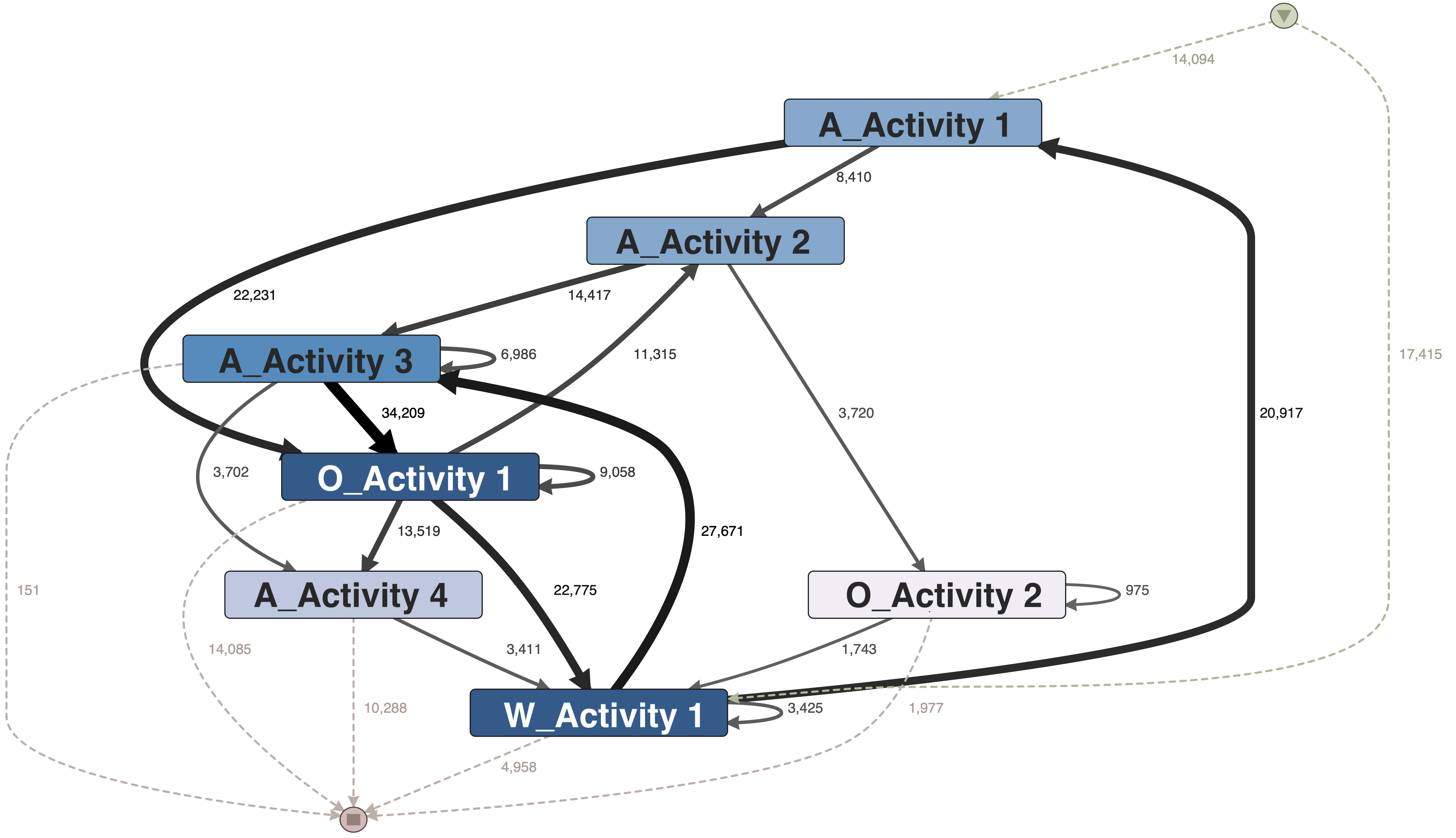
Figure 8: 80/20 DFG of the abstracted loan application log.

Figure 8 depicts the DFG obtained by gecco in this manner, where the activity labels reflect their origin systems. Having grouped the events into seven high-level activities, the DFG shows a considerable reduction in terms of size and complexity. Due to this simplification, we observe clear inter-relations between the different sub-systems. For instance, the process most often starts with the execution of steps in the application-handling system (A_Activity 1 to 3), followed by a part in the offer system (O_Activity 1), and again concluded in the application-handling system (A_Activity 4). Next to this main sequence, the workflow-related steps (W_Activity 1) occur in parallel to the other activities, whereas the refusal of an offer (O_Activity 2) represents a clear alternative path.

It is important to stress that such insights are only possible due to the constraint-driven nature of our work. In fact, when applying gecco without imposing any constraints, the intertwined nature of the process even yielded high-level activities that contain events from all three sub-systems, thus obfuscating the key inter-relations in the process.

VII Related Work

Our work primarily relates to the following streams:

Log abstraction in process mining. In the context of process mining, a broad range of techniques have been developed for log abstraction, also referred to as event abstraction, of which Van Zelst et al. [VanZelst2020] and Diba et al. [Diba2020] recently provided comprehensive overviews. Unsupervised techniques mostly employ clustering [folino2015mining, rehse2018clustering] or generic abstraction patterns [bose07, Wiegand2021] to group low-level events into high-level activities. Other techniques are supervised, requiring users to provide information about the high-level activities to be discovered, captured ,e.g., in the form of a process model [baier2014bridging], specific event annotations [Leemans20], or domain hierarchies [klessascheck].

Compared to gecco, existing unsupervised techniques do not guarantee any characteristics for the abstracted logs, which can result in a considerable loss of information (cf., § VI-D) , while the supervised techniques require a user to explicitly specify how abstraction should be performed, whereas our work only needs a specification of what properties they desire.

Behavioral pattern mining from event logs. Behavioral pattern mining also lifts low-level events to a higher degree of abstraction by identifying interesting patterns in event logs, including constructs such as exclusion, loops, and concurrency. Local Process Models (LPMs) [Tax2016] provide an established foundation for this. LPMs are mined according to pattern frequency, while extensions have been proposed to employ interest-aware utility functions [Tax2018] and incorporate user constraints [Tax2018a]. Behavioral pattern mining has been also addressed through the discovery of maximal and compact patterns in logs [Acheli2019] and their context-aware extension [acheli21].

While their purposes are similar, a key difference between behavioral pattern mining and log abstraction is that the former cherry-picks interesting parts from an event log, whereas the latter strives for comprehensive abstraction over an entire log.

Sequential pattern mining. Approaches for sequential pattern mining [agrawal1995mining, pei2004mining] identify interesting patterns in sequential data. As for LPMs, interesting is typically defined as frequent [han2007frequent], while techniques for high-utility sequential pattern mining also support utility functions specific to the data attributes of events [truong2019survey, yin2013efficiently, yin2012uspan]. Cohesion, comparable to distance measures used in log abstraction, has also been applied as a utility measure for pattern mining in single long sequences [cule2009, Cule2016]. Furthermore, research in constrained sequential pattern mining primarily focuses on exploiting constraint characteristics such as monotonicity to improve efficiency [Pei2007], which we leverage during the first step of our approach as well. Frequently the focus is on specific constraints, e.g., time-based gap constraints [agoa2017].

In contrast to gecco, pattern mining techniques do not consider concurrency and exclusion. Moreover, like for behavioral pattern mining, the focus is on the identification of individual patterns, while our work strives for global abstraction.