Estimating the Value-at-Risk by Temporal VAE

Abstract

Estimation of the value-at-risk (VaR) of a large portfolio of assets is an important task for financial institutions. As the joint log-returns of asset prices can often be projected to a latent space of a much smaller dimension, the use of a variational autoencoder (VAE) for estimating the VaR is a natural suggestion. To ensure the bottleneck structure of autoencoders when learning sequential data, we use a temporal VAE (TempVAE) that avoids an auto-regressive structure for the observation variables. However, the low signal-to-noise ratio of financial data in combination with the auto-pruning property of a VAE typically makes the use of a VAE prone to posterior collapse. Therefore, we propose to use annealing of the regularization to mitigate this effect. As a result, the auto-pruning of the TempVAE works properly which also results in excellent estimation results for the VaR that beats classical GARCH-type and historical simulation approaches when applied to real data.

Keywords: Value-at-Risk, variational autoencoders, recurrent neural networks, risk-management, auto-pruning, posterior collapse

1 Introduction

The value-at-risk (VaR) is the most prominent risk measure in finance. Being defined as a typically high quantile of the loss function of a portfolio of assets over a fixed time horizon, it is notoriously hard to estimate. Methods to determine it range from simple historical simulation to parametric approximation, in particular variants of GARCH-models combined with conditional normal distribution assumptions (see e.g. Engle (2012)), to first applications of neural networks (see e.g. Chen et al. (2009)).

In this work, we propose the temporal variational autoencoder (TempVAE), a variational recurrent neural network (VRNN) designed to handle the low signal-to-noise ratio in financial time series, and apply it to VaR estimation. By leaving out an auto-regressive structure for the observation variables, we explicitly force the model to use the bottleneck structure from autoencoders.

The key concept behind the TempVAE is the variational autoencoder (VAE; see Kingma et al. (2014) and Rezende et al. (2014)). VAE produce stochastic latent representations as opposed to standard autoencoders (AE) which yield deterministic ones. The result of the distribution model is a more meaningful latent space fragmentation and an increase in robustness against common training pitfalls such as over-fitting or model misspecification.

With the introduction of VRNNs, Chung et al. (2015) show promising results to model complex data sequences, like speech data, as compared to standard RNN models. Based on this work, Luo et al. (2018) propose a neural stochastic volatility model (NSVM) and show that, using VRNN, it is possible to adequately model the volatility of financial data. However, the low signal-to-noise ratio makes variational models prone to posterior collapse, i.e. the encoder becoming independent of the input.

The reason for the posterior collapse is the auto-pruning. During training the net sets nodes for the latent space inactive. This property of variational models is known as a double-edged sword and has been analyzed by various authors (see e.g. Burda et al. (2016) and Sicks et al. (2021)). On the one hand, the model focuses on useful representations by pruning away not needed nodes. On the other hand, it is considered a problem when too many nodes become inactive before learning a useful representation.

As a variational model, the TempVAE is also prone to posterior collapse. We propose to use annealing (see also Bowman et al. (2015)) of the regularization to mitigate this effect. This way, we benefit from the auto-pruning property to find useful representations of sequence data.

Using our new proposed model, we make the following contributions:

1. We show that the TempVAE possesses the auto-pruning property. Given synthetic data, the TempVAE identifies the correct number of latent factors to adequately model the data.

2. For the VaR estimation, we show that our model performs excellent and beats the benchmark models.

The remaining paper is structured as follows. In Section 2, we present related work and compare it to our research. The definition of the TempVAE can be found in Section 3. In Section 4, we explain the data and provide our results for the VaR estimation with the TempVAE. We conclude the paper in Section 5.

2 Comparison to Related Work

Various authors have considered stochastic units in RNNs. Bayer and Osendorfer (2014), Chung et al. (2015) and Fraccaro et al. (2016) propose stochastic RNN with auto-regressive structures for the observations while Goyal et al. (2017) and Luo et al. (2018) extend the approach of Chung et al. (2015) via auxiliary cost terms in the objective or bidirectional RNNs respectively. Moreover Xu and Chen (2021) propose a similar model to Luo et al. (2018) and apply it to financial return data.

Krishnan et al. (2017) consider a Gaussian state space model by assuming the Markov property for the latent variables and excluding auto-regressive structures. Given their assumptions, they show that the true posterior for the latents given the observations only depends on future observations. Additionally, Fraccaro et al. (2017) consider a combination of VAE with a state space model. Specifically, they assume that the observations of the state space model make up the bottleneck of the VAE. This way, they achieve a disentanglement of the latent representation and the dynamics.

Finally, Bowman et al. (2015) consider the encoding and decoding of single layer RNN sequences via VAEs to model speech data. They argue that annealing of the regularization term is needed in order to learn meaningful information passing through the bottleneck.

Alternatively to the models by Chung et al. (2015) and Luo et al. (2018), we model a temporal dependency only in the prior distribution. Therefore, our model is similar to the deep Markov model by Krishnan et al. (2017), but we do not use the Markov assumption.

By excluding the auto-regressive dependency for the observation variables, the return distribution is independent from past returns, but not from past latents. Therefore, we force the encoder of the implemented model to encode as much information as possible in the latents $Z$. As a consequence, properties of conventional VAE like the auto-pruning can work properly. This is not necessarily the case if we model the decoder distribution to be auto-regressive on the returns $R$, as assumed by Luo et al. (2018) and Chung et al. (2015). In this case, a substantial part of the information that can be used by the decoder wouldn’t have to pass the bottleneck. Even if the posterior $q(Z|R)$ collapses and becomes independent of the input, the decoder would be able to use past observed $R$ to achieve a good fit.

Various authors have proposed to estimate the VaR with artificial neural networks (ANN). Liu (2005) uses the estimates of historical simulation and GARCH as input for ANNs. Therefore his model can be interpreted as an ensemble model. Chen et al. (2009) and Arimond et al. (2020) estimate the VaR by modelling parameters of their respective distribution assumption. Chen et al. (2009) use a standard ANN whereas Arimond et al. (2020) compare ANNs with temporal convolutional neural nets and RNNs. Arian et al. (2020) use standard VAE for the task of estimating the VaR. To account for the time dependency in the data, they preprocess the data with rolling window statistics.

By using the TempVAE for this task, we have a time-dependent and, due to the auto-pruning property, parsimonious model for the data sequences. As the joint log-returns often can be projected to a lower dimensional space, estimation of the VaR with this model comes as a natural task.

3 The Temporal Variational Autoencoder

We use the TempVAE to learn the multivariate distribution of asset returns. Therefore, we assume that the return series $R=R_{1:T}$ is generated via latent variables $Z=Z_{1:T}$, where $T\in\mathbb{N}$ and $T>1$. The distributions of the variables $Z_{t}$ are estimated via approximate inference and we expect these to hold information like the current market environment, peer group behaviour or interactions. Given the two discrete-time stochastic processes $R$ and $Z$, we assume an auto-regressive time dependency on the latents, given by

$$Z_{t}|Z_{1:t-1} \sim\mathcal{N}\left(\boldsymbol{\mu}^{z}(Z_{1:t-1}),\boldsymbol{\Sigma}^{z}(Z_{1:t-1})\right),$$ (1)

$$R_{t}|Z_{1:t} \sim\mathcal{N}\left(\boldsymbol{\mu}^{r}(Z_{1:t}),\boldsymbol{\Sigma}^{r}(Z_{1:t})\right),$$ (2)

where $\boldsymbol{\mu}^{z}$, $\boldsymbol{\mu}^{r}$, $\boldsymbol{\Sigma}^{z}$ and $\boldsymbol{\Sigma}^{r}$ are functions mapping to $\mathbb{R}^{\kappa}$, $\mathbb{R}^{d}$, $\mathbb{R}^{\kappa\times\kappa}$ and $\mathbb{R}^{d\times d}$ respectively. Given this dependency structure, the joint distribution can be factorized as

$$p_{\boldsymbol{\theta}}(Z) =\prod_{t=1}^{T}p_{\boldsymbol{\theta}}(Z_{t}|Z_{1:t-1}),$$ (3)

$$p_{\boldsymbol{\theta}}(R|Z) =\prod_{t=1}^{T}p_{\boldsymbol{\theta}}(R_{t}|Z_{1:t}).$$ (4)

To account for the dependency of the past sequences, we use RNN layers. Further do we use Multi-Layer Perceptrons (MLPs) to map from the output of the RNNs to the parameter space of the distributions. In total, we use the model architecture given by

$$\left\{\boldsymbol{\mu}_{t}^{z},\boldsymbol{\Sigma}_{t}^{z}\right\} =\mathrm{MLP}^{z}_{G}\left(h_{t}^{z}\right),$$ (5)

$$h_{t}^{z} =\mathrm{RNN}_{G}^{z}\left(h_{t-1}^{z},Z_{t-1}\right),$$ (6)

$$Z_{t} \sim\mathcal{N}\left(\boldsymbol{\mu}_{t}^{z},\boldsymbol{\Sigma}_{t}^{z}\right),$$ (7)

$$\left\{\boldsymbol{\mu}_{t}^{r},\boldsymbol{\Sigma}_{t}^{r}\right\} =\mathrm{MLP}^{r}_{G}\left(h_{t}^{r}\right),$$ (8)

$$h_{t}^{r} =\mathrm{RNN}_{G}^{r}\left(h_{t-1}^{r},Z_{t}\right),$$ (9)

$$R_{t} \sim\mathcal{N}\left(\boldsymbol{\mu}_{t}^{r},\boldsymbol{\Sigma}_{t}^{r}\right),$$ (10)

which is also depicted in Figure 1. Combining the hidden states of the model is possible and yields a more general model formulation. But during our experiments, we found that it is favourable to have the prior as not trainable (see Appendix B.2). In order to achieve this, we separate the hidden states as shown in Figure 1.

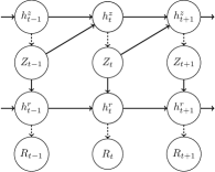
Figure 1: The dependency structure of the generative model. Realizations of $Z$ influence the realizations of $R$ as well as all future realizations of $R$ and $Z$. The Gaussian distribution parameters from the MLP as well as the sampling are represented by the dashed lines. Further, information of former time points is propagated through the RNN hidden states $h^{r}_{\cdot}$ and $h^{z}_{\cdot}$.

We approximate the intractable $p_{\boldsymbol{\theta}}(Z|R)$ by the inference distribution $q_{\boldsymbol{\phi}}(Z|R)$. Similar to Krishnan et al. (2017), one can show that $Z_{t}\mathchoice{\mathrel{\hbox to0.0pt{$\displaystyle\perp$\hss}\mkern 2.0mu{\displaystyle\perp}}}{\mathrel{\hbox to0.0pt{$\textstyle\perp$\hss}\mkern 2.0mu{\textstyle\perp}}}{\mathrel{\hbox to0.0pt{$\scriptstyle\perp$\hss}\mkern 2.0mu{\scriptstyle\perp}}}{\mathrel{\hbox to0.0pt{$\scriptscriptstyle\perp$\hss}\mkern 2.0mu{\scriptscriptstyle\perp}}}R_{1:t-1}|Z_{1:t-1}$. Therefore, we can factorize the distribution such that the variable $Z_{t}$ depends on the (future) observations $R_{t:T}$:

$$p_{\boldsymbol{\theta}}(Z|R)=\prod_{t=1}^{T}p_{\boldsymbol{\theta}}(Z_{t}|Z_{1:t-1},R_{t:T}).$$ (11)

Krishnan et al. (2017) argue that $q$ should be factorized the same way. As $q$ is only an approximation to $p$, we also considered providing the full sequence which yields a better performance (see Appendix B.7). We therefore factorize $q$ as

$$q_{\boldsymbol{\phi}}(Z|R)=\prod_{t=1}^{T}q_{\boldsymbol{\phi}}(Z_{t}|Z_{1:t-1},R_{1:T})$$ (12)

and assume $q_{\boldsymbol{\phi}}(Z_{t}|Z_{1:t-1},R_{1:T})\sim\mathcal{N}\left(\hat{\boldsymbol{\mu}}^{z}(Z_{1:t-1},R_{1:T}),\boldsymbol{\hat{\Sigma}}^{z}(Z_{1:t-1},R_{1:T})\right)$. $\hat{\boldsymbol{\mu}}^{z}$ and $\boldsymbol{\hat{\Sigma}}^{z}$ are functions mapping to $\mathbb{R}^{\kappa}$ and $\mathbb{R}^{\kappa\times\kappa}$ respectively. Furthermore, we implement the inference distribution via a bidirectional RNN as follows

$$\left\{\hat{\boldsymbol{\mu}}_{t}^{z},\boldsymbol{\hat{\Sigma}}_{t}^{z}\right\} =\mathrm{MLP}^{z}_{I}\left(\hat{h}_{t}^{z}\right)$$ (13)

$$\hat{h}_{t}^{z} =\mathrm{RNN}_{I}^{z}\left(\hat{h}_{t-1}^{z},Z_{t-1},\left[\hat{h}_{t}^{\rightarrow},\hat{h}_{t}^{\leftarrow}\right]\right)$$ (14)

$$\hat{h}_{t}^{\rightarrow} =\mathrm{RNN}_{I}^{z}\left(\hat{h}^{\rightarrow}_{t-1},R_{t-1}\right)$$ (15)

$$\hat{h}_{t}^{\leftarrow} =\mathrm{RNN}_{I}^{z}\left(\hat{h}^{\leftarrow}_{t+1},R_{t+1}\right)$$ (16)

$$Z_{t} \sim\mathcal{N}\left(\hat{\boldsymbol{\mu}}_{t}^{z},\boldsymbol{\hat{\Sigma}}_{t}^{z}\right).$$ (17)

As we have a distribution assumption with an intractable $p(Z|X)$, the usual suspect for the model training is the evidence lower bound (ELBO) given as

$$\mathcal{L}(\boldsymbol{\theta},\boldsymbol{\phi}) =\mathbb{E}_{q_{\boldsymbol{\phi}}(Z|R)}\left[\log p_{\boldsymbol{\theta}}(R|Z)\right]+\mathbb{E}_{q_{\boldsymbol{\phi}}(Z|R)}\left[\log\left(\dfrac{p_{\boldsymbol{\theta}}(Z)}{q_{\boldsymbol{\phi}}(Z|R)}\right)\right]$$ (18)

$$=\mathbb{E}_{q_{\boldsymbol{\phi}}(Z|R)}\left[\log p_{\boldsymbol{\theta}}(R|Z)\right]-D_{KL}\left(q_{\boldsymbol{\phi}}(Z|R)||p_{\boldsymbol{\theta}}(Z)\right).$$ (19)

The components are given by equations (3), (4) and (12). As we have $\log p_{\boldsymbol{\theta}}(R)\geq\mathcal{L}(\boldsymbol{\theta},\boldsymbol{\phi})$, maximization of the ELBO most likely leads to an increase in the likelihood of our distribution model. In a similar way to Krishnan et al. (2017), we can rewrite the ELBO as

$$\small\mathcal{L}(\boldsymbol{\theta},\boldsymbol{\phi})=\mathbb{E}_{q_{\boldsymbol{\phi}}(Z|R)}\left[\log p_{\boldsymbol{\theta}}(R|Z)\right]-\sum_{t=1}^{T}\mathbb{E}_{q_{\boldsymbol{\phi}}(Z_{1:t-1}|R)}\Big{[}D_{KL}\big{(}q_{\boldsymbol{\phi}}(Z_{t}|Z_{1:t-1},R)\>\big{\lVert}\>p_{\boldsymbol{\theta}}(Z_{t}|Z_{1:t-1})\big{)}\Big{]}.$$ (20)

Since we assume a Gaussian distribution for $q$ and $p$, we can analytically calculate the Kullback-Leibler divergence (KL-Divergence) inside the expectation in (20). We approximate the outer expectations numerically by Monte Carlo.

3.1 The Auto-Pruning Property of VAEs and the Posterior Collapse

The auto-pruning of VAE originates from the KL-Divergence and has been analyzed by various authors (see Burda et al. (2016) and Sicks et al. (2021)). When nodes in the bottleneck are “pruned away”, it means that these nodes are not used in the neural net and therefore also not for the reconstruction. The auto-pruning capabilities of VAE are desirable, as the model focuses on useful latent representations. However, it is considered a problem when too many units become inactive before learning such a useful representation. In the extreme case, the KL-Divergence between $q_{\boldsymbol{\phi}}(Z|R)$ and $p_{\boldsymbol{\theta}}(Z)$ is 0 and we have $q_{\boldsymbol{\phi}}(Z|R)\equiv p_{\boldsymbol{\theta}}(Z)$. $q$ is independent of $R$ and we say that the posterior $q$ collapses as the input does not matter.

As we consider multivariate Gaussian distributions with diagonal covariance, it becomes apparent that only a subset of nodes can be inactive. The posterior does not collapse in this case, as information can still be propagated to the decoder through active nodes.

When using the TempVAE on financial data, we observe an instantaneous collapse of the posterior at the beginning of the training. In our point of view, the signal within the financial returns data is not strong enough to be captured before the KL-Divergence term dominates the ELBO and causes a posterior collapse. Therefore, we consider $\beta$-annealing of the KL-Divergence similar to Bowman et al. (2015) (see Appendix A).

To measure the amount of active units, Burda et al. (2016) propose an activity statistic that is calculated after training. For each node, they estimate the activity by

$$A_{u}=\mathrm{Cov}_{x}\left(\mathbb{E}_{q_{\phi}\left(u|x\right)}[u]\right)$$

and call a node inactive, if $A_{u}<0.01$. Since we assume a time-dependent model for the prior in (3), we adjust the activity statistic to calculate the activities of a sequence of $Z_{1:M}\in\mathbb{R}^{M\times\kappa}$. For $m=1,\ldots,M$ and $k=1,\ldots,\kappa$ we calculate

$$A_{z}^{(m,k)}:=\mathrm{Cov}_{R,Z_{1:m-1}}\left(\mathbb{E}_{q_{\phi}\left(Z_{m,k}|Z_{1:m-1},R\right)}\left[Z_{m,k}\right]-\mathbb{E}_{p_{\theta}\left(Z_{m,k}|Z_{1:m-1}\right)}\left[Z_{m,k}\right]\right).$$ (21)

The statistic becomes equal to the one proposed by Burda et al. (2016), if we assume a time-independent standard Gaussian prior in (3). With the statistic in (21) we quantify the effect of the input $R$. Similar to Burda et al. (2016), we call a node inactive from the input, if $A_{z}^{(m,k)}<0.01$.

4 Implementation and Experiments

In this section, we present the results we achieved on four data sets (see Sections 4.1) with our model regarding the identification of the underlying signal (see Section 4.2). Then, in Section 4.3 we present results for the fit to financial data as well as the VaR estimation. For further details on the model implementation and for an additional ablation study validating our design choices see Appendices A and B.

4.1 Description of employed Data Sets

We consider the four data sets “DAX”, “S&P500”, “Noise” and “Oscillating PCA” for our studies. Throughout the section, data is stored in $d$-dimensional vectors

$$R_{t}:=\left(R_{t,1},\ldots,R_{t,d}\right)^{T}\in\mathbb{R}^{d}.$$ (22)

First, we consider ($d$=22) stock price time series, provided by DAX (German stock index) enlisted companies, from 11.06.2001 to 09.06.2021. We calculate the daily logarithmic returns via the observed close prices. Therefore, if $S_{t,i}$ denotes the price of stock $i=1,\ldots,d$ at time $t=1,\ldots,T$, the data set “DAX” contains

$$R_{t,i}:=\ln\left(S_{t,i}\right)-\ln\left(S_{t-1,i}\right).$$ (23)

For “S&P500”, we consider 397 stocks of the S&P500 index that have a history from 02.01.2002 up to 09.06.2021. We calculate the log-returns analogously to the “DAX” data.

The data set “Noise” is just white noise with dimension $d=22$. Hence, for all $t=1,\ldots,T$ and $i=1,\ldots,d$

$$R_{t,i}\sim\mathcal{N}\left(0,1\right).$$

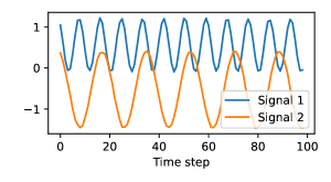
Figure 2: The first 100 steps of two oscillating signals. The two signals have different amplitude, frequency and origin.

The data set “Oscillating PCA $k$” (with $k\in\{2,5,10\}$) is constructed based on $k$ independent harmonic oscillator signals. Each univariate signal $Z_{1:T}$ is constructed by randomly choosing an intercept $i\sim\pazocal{U}\left(-1,1\right)$, an amplitude $a\sim\pazocal{U}\left(-1,1\right)$, a frequency $f\sim\pazocal{U}\left(0.5,24\right)$ and a noise series $\epsilon_{1:T}$, with $\epsilon\sim\mathcal{N}\left(0,0.02^{2}\right)$. Then, we set

$$Z_{t}=i+a\cdot\cos\left(\dfrac{t}{100}\cdot f\cdot\pi\right)+a\cdot\epsilon_{t}.$$

The case $k=2$ is shown in Figure 2. The oscillator sequences $Z_{1:T,1:k}\in\mathbb{R}^{T\times k}$ are then transformed to a 22-dimensional series by applying a randomly chosen rotation $U\in\mathbb{R}^{d\times k}$:

$$S_{t}=U\cdot Z_{t,1:k}^{T}+5\qquad\text{and}\qquad R_{t,i}:=\ln\left(S_{t,i}\right)-\ln\left(S_{t-1,i}\right)$$

for each $t=1,\ldots,T$ and $i=1,\ldots,d$.

Finally, a sliding window is applied to the $d$-dimensional series $R_{1:T}$ to generate $T-M$ consecutive series in $\mathbb{R}^{d\times M}$ of size $M=21$. For further details on preprocessing procedures, see Appendix A.

4.2 Signal Identification

We train the TempVAE on the four data sets from Section 4.1 and analyze calculated activities given by (21) as well as the fit to the data. As we can see in Figure 3 and 4, the TempVAE correctly identifies the amount of hidden dimensions. For the “Noise” data, no activity is reported at all. The decoder model $p(R|Z)$ is left on it’s own to model the data as no meaningful information can be identified that can be propagated from input to output. For the data “Oscillating PCA 2”, the model correctly identifies the two active nodes per time step. For the “Oscillating PCA 5” and “Oscillating PCA 10” data, the model also identifies two active dimensions through time (see Appendix D). Though this is not the amount given by the linear construction, identifying less dimensions is not necessarily problematic since we have a non-linear model. We observe comparable fitting results for these data sets (see Appendix D).

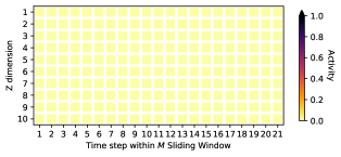
Figure 3: The activity statistics for the “Noise” data. We consider sequences of size $M=21$ as input. Depicted are the activity values of statistic (21) for the $\kappa=10$ dimensional latent space.

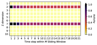
Figure 4: The activity statistics for the “Oscillating PCA 2” data. We consider sequences of size $M=21$ as input. Depicted are the activity values of statistic (21) for the $\kappa=10$ dimensional latent space.

Applied to the financial data, we can observe two and four active dimensions for the “DAX” and “S&P500” data sets respectively (see Appendix E). The fact that only a few active nodes could be identified is not surprising. In their work Laloux et al. (2000) show that only a small fraction of dimensions (roughly 11) are needed to linearly model 406 assets of the S&P500 during the years 1991-1996.

4.3 Fit to Financial Data and Application to Risk Management

To assess the performance of the model on the “DAX” data, we compare the TempVAE to a GARCH model as well as to the multivariate GARCH versions DCC-GARCH-MVN and DCC-GARCH-MVt (see Appendix C for details). Therefore, we calculate the negative log-likelihood (NLL), given by

$$\mathrm{NLL}(R_{t}^{\text{nonlog}},\mu_{t},\Sigma_{t}):=\frac{1}{2}\left(\kappa\log\left(2\pi\right)+\log\left|\Sigma_{t}\right|+\left(R_{t}^{\text{nonlog}}-\mu_{t}\right)^{T}\Sigma_{t}^{-1}\left(R_{t}^{\text{nonlog}}-\mu_{t}\right)\right)$$

and average across all timestamps in the test set. $R_{t}^{\text{nonlog}}$ are the non-logarithmic returns of the test data and $\mu_{t}$ as well as $\Sigma_{t}$ are estimated by the models. To estimate these values, we first sample the log-returns from a model. For the TempVAE, we estimate these empirically by sampling

$$z_{1:t}^{(i)}\sim q_{\phi}(Z|r_{1:t-1})\quad\text{ as well as }\quad r_{t}^{(i)}\sim p_{\boldsymbol{\theta}}(R|z_{1:t}^{(i)})$$

for $i=1,\ldots,1000$. Then, we transform these samples to nonlog-returns and calculate the empirical means and covariances to approximate $\mu_{t}$ and $\Sigma_{t}$.

We also consider the diagonal NLL, where we use the diagonal matrix with entries $\textnormal{diag}\left(\Sigma_{t}\right)$ instead of $\Sigma_{t}$. Further do we calculate a univariate version by considering the returns of an equally weighted portfolio containing the 22 assets. Given the log-returns in (23), we calculate these by

$$R_{t,i}^{P,\text{nonlog}}:=\dfrac{1}{d}\sum_{i=1}^{d}\left(\exp\left(R_{t,i}\right)-1\right).$$ (24)

Model	Diagonal NLL	NLL	Portfolio NLL
GARCH	22.76	22.84	-0.51
TempVAE	25.79	20.35	-3.04
DCC-GARCH-MVN	25.03	18.69	-3.07
DCC-GARCH-MVt	25.44	19.17	-3.05

Table 1: Fit scores for models TempVAE, GARCH and two multivariate GARCH. In all cases, lowest is best.

Table 1 displays the different fit scores for the three models. Considering the NLL scores, the GARCH and normal DCC-GARCH models achieve the best performance since these models are directly minimizing the respective scores. The TempVAE as a regularized model has to find a trade-off between the NLL and the regularization terms. Nonetheless, if we consider the scores for the portfolio returns, we see all multivariate models performing similarly and outperforming the GARCH model. Due to the strong dependency between the different assets in the portfolio, estimating the underlying covariance structure plays an essential role in estimating the next day’s portfolio performance. Further, we could observe the models capturing the correlations between the assets (see Appendix F for an excerpt of the first two dimensions).

To compare the performance on the VaR estimation, as a further method we consider historical simulation (HS). We calculate the VaR estimates via 1000 Monte Carlo samples from the respective distributions. The VaR95 is then the 50th of the ordered samples and the VaR99 the 10th sample. We evaluate these with the ‘Regulatory Loss Function’ (RLF) proposed by Sarma et al. (2003) which penalizes exceedance of the VaR and is given by

$$\mathrm{RLF}\left(\textnormal{VaR}_{t},r_{t}\right)=\begin{cases}\left(\textnormal{VaR}_{t}-r_{t}\right)^{2},&\text{if }r_{t}\geq\textnormal{VaR}_{t}\\ 0,&\text{otherwise.}\end{cases}$$

We calculate the average of these values over the test set.

Model	RLF95	RLF99	Br95	Br99
GARCH	44.47	32.35	24.3	17.8
TempVAE	12.64	5.96	4.8	1.3
DCC-GARCH-MVN	13.15	7.10	5.4	2.1
DCC-GARCH-MVt	10.23	4.14	3.9	0.6
HS	14.57	7.43	5.1	1.3

Table 2: The table displays the values (all of these have to be multiplied by $10^{-6}$) of the RLF scores as well as the average count of breaches for the VaR95 and the VaR99 within the test set. For the RLF values, lowest is best. For the average breaches, the respective quantile assumption is the optimal value. Hence for VaR95 the best value is 5 and for VaR99 the best value is 1.

In Table 2, the losses for the models as well as the average number of breaches are displayed. The amount of average breaches helps us to validate the VaR estimates by their 5% and 1% quantile assumption and a good performance is a necessary condition. As the RLF can be simply minimized to zero by decreasing any VaR estimates, we only compare models in their RLF that show a reasonable amount of breaches. Therefore, though DCC-GARCH-MVt has the lowest values for the RLF95 and RLF99, the TempVAE produces the best estimates.

In Figure 5, the VaR95 values for the DCC-GARCH-MVN, HS and TempVAE are displayed. The full path of the VaR95 estimates as well as the VaR99 estimates can be found in Appendix F. We can see the VaR95 estimates for the DCC-GARCH-MVN and TempVAE are quickly responding to the changes in the volatility of the data. Comparing TempVAE directly to DCC-GARCH-MVN, we see the VaR estimates to be more volatile but also responsive to the evolution of the returns. The HS on the other side is showing the well-known time-delay (see Liu (2005)). Even though in terms of average breaches the HS is best followed by TempVAE, in our point of view the TempVAE provides the most reasonable estimates among the models.

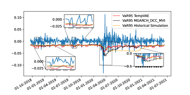
Figure 5: The VaR95 estimates for the two models TempVAE, DCC-GARCH-MVN and HS on a fraction of the test data.

5 Conclusion

In this paper, we present a novel variational recurrent neural net with bottleneck structure known to autoencoders to handle sequential data. As we model the data on the basis of a time-dependent prior, we call the model temporal variational autoencoder (TempVAE). By ensuring that the information has to flow through the bottleneck, we leverage the auto-pruning property known to VAE. This way, we are able to find parsimonious model representations of the data, without using methods like grid search.

We successfully apply the TempVAE to risk management. More precisely, we estimate the risk measure VaR and show that our model performs competitive to the considered benchmark models. We show that, expecting reasonable amount of VaR breaches, the model is performing best in terms of the considered RLF scores.

Future research directions can incorporate applying the TempVAE architecture to other types of data sequences. Furthermore, the active dimensions in the bottleneck are not necessarily yielding disentangled representations. Research in this direction can foster the understanding of the auto-pruning and hence variational models further.

A $\beta$-Annealing, Model Implementation and Data Preprocessing

A.1 $\beta$-Annealing

The low signal-to-noise ratio in financial data makes it necessary to proceed delicately when modelling financial data. We propose to use annealing of the regularization to mitigate the initial effects of the auto-pruning. Specifically, we consider $\beta$-annealing of the KL-Divergence similar to Bowman et al. (2015). We add $\beta\geq 0$ to the ELBO in (20) to get

$$\scriptstyle\mathcal{L}_{\beta}(\boldsymbol{\theta},\boldsymbol{\phi})=\mathbb{E}_{q_{\boldsymbol{\phi}}(Z|R)}\left[\log p_{\boldsymbol{\theta}}(R|Z)\right]-\beta\cdot\sum_{t=1}^{T}\mathbb{E}_{q_{\boldsymbol{\phi}}(Z_{1:t-1}|R)}\Big{[}D_{KL}\big{(}q_{\boldsymbol{\phi}}(Z_{t}|Z_{1:t-1},R)\>\big{\lVert}\>p_{\boldsymbol{\theta}}(Z_{t}|Z_{1:t-1})\big{)}\Big{]}.$$ (25)

The KL influence is adjusted over $\beta$. During training we start with $\beta=0$ and increase it over time. In Figure 6, the annealing over 1000 epochs is depicted as well as the effect on the KL-Divergence is shown.

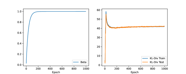
Figure 6: On the left: The KL influence is adjusted over $\beta$. During training we start with $\beta=0$ and increase it over time. We implement this by subtracting an exponentially decaying term from the ultimate $\beta$ value. We use a decay rate of $0.96$ and decay steps $20$. On the right: The evolution of the (negative) KL-Divergence over time. We can see how the values starts to decrease after the annealing has increased $\beta$ enough.

A.2 Model Implementation

We implement the model based on Section 3. For the RNN’s we choose ‘Gated Recurrent Units’ (see Cho et al. (2014)) with dimension 16 and for the MLP’s we use normal Feedforward Networks that have two hidden layers with dimension 16 and the output layer with varying output dimension. For the latent variables we choose dimension 10. In our experimens, with this size of the latent dimension the model is overspecified and the auto-pruning removes not needed dimensions.

We initialize all MLP layer weights with the ‘Variance Scaling’ initializer as proposed by He et al. (2015). As activation function for the hidden layers we use the ‘Rectified Linear Unit’ (ReLU). For the $\boldsymbol{\mu}^{z}$, $\hat{\boldsymbol{\mu}}^{z}$ and $\boldsymbol{\mu}^{r}$ layer we use no activation. We use a diagonal covariance structure for $\boldsymbol{\Sigma}^{z}$ and $\boldsymbol{\hat{\Sigma}}^{z}$ and a rank-1 perturbation output as given in Rezende et al. (2014) for $\boldsymbol{\Sigma}^{r}$. For all covariance layers, we use exponential activation for the diagonal entries. Further, we add L2 regularization with parameter $\lambda=0.01$ for the weights of the hidden layers of the MLP as well as dropout with a rate of $10\%$ to the RNN layers. In our experiments, both the dropout and the L2 regularization turned out to be crucial for the auto-pruning to work properly as well as for an adequate data modelling (see Appendix B.6).

In contrast to the model of Luo et al. (2018), we set the parameters of the prior (i.e. equations (5) - (7)) as non-trainable. Allowing a trainable prior results in an unfavourable performance regarding the signal identification as well as the risk-management application (see Appendix B.2). In our point of view, the fixed prior serves as guidelines for the model to identify temporal transitions. If the prior is learned simultaneously with the encoder, past adaptions of the encoder to the temporal dynamics can become obsolete by changes in the prior parametrization.

For the training of the model, we use the reparametrization trick as introduced by Kingma and Welling (2014). To approximate both expectations in (20), we use Monte Carlo with one sample. Using the ADAM optimizer by Kingma and Ba (2015), we train the model for $1000$ epochs with a batch size of 256. We use an initial learning rate of $0.001$ with an exponential learning rate decay with decay rate $0.96$ and $500$ decay steps. If not explicitly excluded, we apply the $\beta$-annealing as described in Figure 6 during training.

A.3 Data Preprocessing

To model the data with artificial neural networks, we split the data into a training and test set. Further do we use the empirical mean and standard deviation of the training part to standardize each ($i=1,\ldots,d$) univariate series $R_{1:T,i}$. Finally, we apply a sliding window on the $d$-dimensional series in (22) to generate $T-M$ intervals of size $M=21$. We define

$$R_{t:t+M}:=\left(R_{t},\ldots,R_{t+M}\right)\in\mathbb{R}^{d\times M},$$

for $t=1,\ldots,T-M$. After the preprocessing, we have different amounts of observations which we split into 66% training and the rest test data:

• For the DAX data 5061 observations were split at $t=3340$ into 3340 training observations and 1721 test observations.

• For the S&P500 data 4872 observations were split at $t=3215$ into 3215 training observations and 1657 test observations.

• For the noise data 5050 observations were split at $t=3333$ into 3333 training observations and 1717 test observations.

• For each of the oscillating PCA data sets 9979 observations were split at $t=6586$ into 6586 training observations and 3393 test observations.

B Ablation studies

In this section, we validate some of the design choices for the TempVAE model. We will address each point in a separate section, starting of with the $\beta$-annealing.

B.1 Preventing Posterior Collapse with $\beta$-annealing

A deep neural net like the TempVAE has to be trained with caution to prevent posterior collapse. The $\beta$-annealing proposed in Appendix A is a useful tool to prevent this collapse. In this section, we compare the TempVAE with a model ‘TempVAE noAnneal’ with no annealing, where we set $\beta=1$ instead of using $\beta$-annealing. Given the activity statistics of a model $A_{z}^{(m,k)}$, as described in (21) for $m=1,\ldots,M$ and $k=1,\ldots,\kappa$, we calculate the average count of active units as

$$\bar{A}_{z}:=\dfrac{1}{M\cdot\kappa}\sum_{m=1}^{M}\sum_{k=1}^{\kappa}\mathds{1}_{\left\{A_{z}^{(m,k)}\geq 0.02\right\}}$$ (26)

In Table 3, we see the average count of active units for the two models and in Table 4, the NLL scores as calculated in Section 4.3 are reported.

	DAX	Noise	Osc. PCA 2	Osc. PCA 5	Osc. PCA 10
TempVAE	20%	0%	20%	20%	20%
TempVAE noAnneal	0%	0%	10%	20%	10%

Table 3: The average count of active units given by (26) for the two models with and without annealing. We see that the model with the annealing is not decreasing the number of average active dimensions when increasing the number of latent signals. For the model without annealing this is not the case.

	DAX	Noise	Osc. PCA 2	Osc. PCA 5	Osc. PCA 10
TempVAE	20.29	31.48	-38.51	-1.40	11.07
TempVAE noAnneal	27.49	31.44	3.58	2.60	13.28

Table 4: The negative log-likelihood for the two models on the test set. We see the TempVAE is outperforming the version without annealing on every relevant data set. Only for the noise case, where there is nothing to learn, the results are comparable.

Using the annealing, a latent process in financial data is identified. Without annealing, a posterior collapse occurs and no encoding information is propagated to the decoder. Notice that the amount of active dimensions need not match the amount of latent signals. Because of non-linearities it can be possible for the model to use less dimensions than needed to adequately model the data (see Appendix D).

B.2 Comparison to a Model with Trainable Prior Parameters

Allowing a trainable prior distribution $p_{\boldsymbol{\theta}}(Z)$ yields unfavourable performance regarding the auto-pruning as well as a worse fit to the data. In this section, we find that using a non-trainable prior $p_{\boldsymbol{\theta}}(Z)$ yields better results in terms of the auto-pruning functionality as well as of the fit of the model. To see this, we compare the TempVAE model with a version ‘TempVAE trainPrior’, where the prior is trainable. Figure 7 and 8 display the activities of the ‘TempVAE trainPrior’ bottleneck for the DAX data and for the Oscillating PCA data respectively.

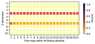
Figure 7: The activity statistics for the “DAX” data for the model ‘TempVAE trainPrior’. We consider sequences of size $M=21$ as input. Depicted are the activity values of statistic (21) for the $\kappa=10$ dimensional latent space.

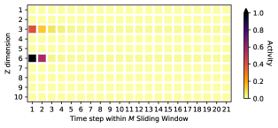
Figure 8: The activity statistics for the “oscillating PCA” data for the model ‘TempVAE trainPrior’. We consider sequences of size $M=21$ as input. Depicted are the activity values of statistic (21) for the $\kappa=10$ dimensional latent space.

Comparing these figures with Figure 4, we notice that the value of the activity statistics drastically decreased. For the model with trainable prior, it is questionable if any information from the input is propagated to the output for the ‘Oscillating PCA’ data at later time steps.

Comparing the VaR forecasts of both models in Figure 9, we see that the VaR forecasts for the model with trainable prior are more volatile. This also affects the average amount of breaches of this estimator as can be seen in Table 5. The TempVAE outperforms the version with trainable prior, as the amount of breaches for the VaR95 should be close to 5 and for VaR99 to 1. In our point of view, setting the prior as non-trainable gives the model more stability during training. This results in a more consistent output e.g. for the VaR estimates.

Model	Br95	Br99
TempVAE	4.8	1.3
TempVAE trainPrior	8.2	3.1

Table 5: The count of average breaches for the model TempVAE and the version with trainable parameters for the prior $p_{\boldsymbol{\theta}}(Z)$. TempVAE outperforms the trainable prior version. For the average breaches, the respective quantile assumption is the optimal value. Hence for VaR95 the best value is 5 and for VaR99 the best value is 1.

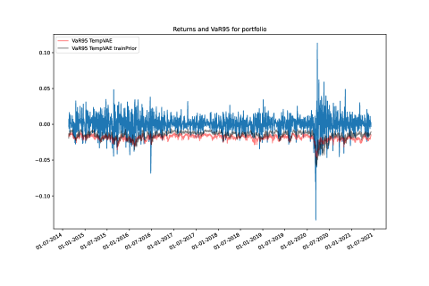
Figure 9: VaR95 forecasts of both models ‘TempVAE’ and ‘TempVAE trainPrior’ on the test set. The VaR forecasts for the model with trainable prior are more volatile.

B.3 Auto-Regressive Structure for the Observables Distribution

Modelling an auto-regressive connection for the observations produces questionable results due to over-fitting. In this section, we compare the model TempVAE with a the model ‘TempVAE AR’, a version of the model with auto-regressive structures as proposed, e.g. by Chen et al. (2020) or Luo et al. (2018). The implementation of the model ‘TempVAE AR’ is identical to the model TempVAE except for the generative distribution. Instead of (8)-(10), we implement this part as

$$\left\{\boldsymbol{\mu}_{t}^{r},\boldsymbol{\Sigma}_{t}^{r}\right\} =\mathrm{MLP}^{r}_{G}\left(h_{t}^{r}\right),$$ (27)

$$h_{t}^{r} =\mathrm{RNN}_{G}^{r}\left(h_{t-1}^{r},z_{t},r_{t-1}\right),$$ (28)

$$r_{t} \sim\mathcal{N}\left(\boldsymbol{\mu}_{t}^{r},\boldsymbol{\Sigma}_{t}^{r}\right).$$ (29)

Therefore, past observations are influencing the current distributions. If such a dependency structure is assumed given a sequence of observations $R_{1:T}$, the latent variables become dependent on the whole observed sequence, as argued in Luo et al. (2018). As we account for this already in our proposed model for the encoder (see (13)-(17)), we do not have to adapt for this part.

Looking at Table 6, we see that TempVAE outperforms ‘TempVAE AR’ on all test sets. In fact, we can observe overfitting for the ‘TempVAE AR’ model whereas the TempVAE did not suffer from this. Common VAE possess an inherent robustness against overfitting (see e.g. Kingma et al. (2014)) originating from the regularization with the KL-Divergence. As the structure of the TempVAE enforces this regularized bottleneck structure, we are not surprised that we do not observe overfitting with the TempVAE. On the other side, ‘TempVAE AR’ has the possibility to ignore the regularized bottleneck and hence overfitting becomes more of a concern.

	DAX	Noise	Osc. PCA (2)	Osc. PCA (5)	Osc. PCA (10)
TempVAE	20.29	31.48	-38.51	-1.40	11.07
TempVAE AR	22.68	32.91	-34.72	25.33	69.26

Table 6: The negative log-likelihood for the two models TempVAE and ‘TempVAE AR’ on the test set. We see the TempVAE is outperforming the version with auto-regressive structure, even in the case of the Noise data set. This is because the ‘TempVAE AR’ model was overfitting this data.

Apart from these results, another point speaks in favor of the TempVAE without auto-regressive structure for the observations. As information does not necessarily has to pass the bottleneck, analyzing the latent space activity becomes tedious. Even for a completely collapsed posterior $q$ the model can use information from the input sequence to model the output.

B.4 Using a Diagonal Covariance Matrix $\boldsymbol{\Sigma}^{r}_{t}$

Here, we compare the ‘TempVAE’ with the model ‘TempVAE diag’, a version of the model, where the output covariance matrix for the observables is modelled as diagonal and not via the rank-1-perturbation as given in Appendix A. As we can see in Table 7, the average amount of VaR breaches is approximately the same for the two model architectures. This indicates that by the usage of the latent variables the covariance structure of the data can be explained well enough to get a comparable performance for the VaR estimates. We still decided to propose the rank-1 perturbation for the model, as Luo et al. (2018) were able to improve their fit this way.

Model	Br95	Br99
TempVAE	4.8	1.3
TempVAE diag	5.3	1.6

Table 7: The count of average breaches for the model TempVAE and the version with diagonal covariance matrix for $\boldsymbol{\Sigma}^{r}_{t}$. For the average breaches, the respective quantile assumption is the optimal value. Hence for VaR95 the best value is 5 and for VaR99 the best value is 1.

B.5 Setting $\boldsymbol{\mu}^{r}_{t}\equiv 0$

In their paper, Xu and Chen (2021) motivate to model only the covariance $\boldsymbol{\Sigma}^{r}_{t}$ of the observable distribution (2). We therefore compare the TempVAE with the model ‘TempVAE zeroMean’, the same model but with the mean parameter fixed to an output of zero. Figure 10 and 11 show the activity statistics for the “DAX” and “Oscillating PCA 2” datasets.

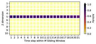
Figure 10: The activity statistics for the “DAX” data for the model ‘TempVAE zeroMean’. We consider sequences of size $M=21$ as input. Depicted are the activity values of statistic (21) for the $\kappa=10$ dimensional latent space.

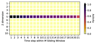
Figure 11: The activity statistics for the “Oscillating PCA 2” data for the model ‘TempVAE zeroMean’. We consider sequences of size $M=21$ as input. Depicted are the activity values of statistic (21) for the $\kappa=10$ dimensional latent space.

Here, we can observe that the number of identified active nodes per timestep is less in comparison with the TempVAE model. A smaller latent space occupation than given by the amount of latent signals is possible due to non-linearities of the net. But in our point of view, it is rather questionable that one latent dimension suffices to capture the signal in both the “Oscillating PCA 2” dataset and the “DAX” dataset. Further, comparing the kernel density estimated distributions of the “Oscillating PCA 2” dataset in Figure 12 and 17, we see that the model is not able to correctly model the two dimensions of the signal inherent in the data. Therefore, we decide to model the mean parameter.

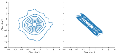
Figure 12: The kernel density estimated distribution of the “oscillating PCA 2” data. On the left we see the model ‘TempVAE zeroMean’ and on the right the historical data.

B.6 Regularization: L2, Dropout and KL-Divergence

In this section, we compare the TempVAE to five other models where different regularization procedures are set inactive. The models we consider are

1. ‘TempVAE’

2. ‘TempVAE det’: The KL-Divergence is switched off and the bottleneck uses only a mean parameter whereas the covariance is set to zero. Therefore, the bottleneck is deterministic and the auto-pruning switched off.

3. ‘TempVAE no dropout/L2’: Dropout and L2 regularization are switched off.

4. ‘TempVAE no L2’: L2 regularization is switched off.

5. ‘TempVAE no dropout’: Dropout is switched off.

6. ‘TempVAE det no dropout/L2’: ‘TempVAE det’ and ‘TempVAE no dropout/L2’ combined.

In Table 8, the average count of active dimensions is shown. As we can see, only the model ‘TempVAE’ is providing favourable results. The deterministic models show no auto-pruning for the Oscillating PCA data versions while the model ‘TempVAE det no dropout/L2’ is even activating most of the latent nodes when modeling the Noise data. This extensive use of bottleneck nodes is a sign of overfitting. It is important to understand that if the KL-Divergence is switched off for these models, the reconstruction error, that is, the first term in equation (25), is the only factor driving the encoder model training. Hence, the encoder aims to provide latent variables that are best suited for reconstruction just as in a normal autoencoder model. Since encoder and prior distribution are disconnected without the KL-Divergence term, the forecast of these models is highly doubtful. Nonetheless the reconstruction has been learned and therefore we can analyze the latent space activity.

The stochastic models without L2, dropout or both also show questionable results. Therefore, we conclude that both regularizations are essential to learn the deep neural net and for the auto-pruning to work properly.

Model	dax	noise	oscPCA2	oscPCA5	oscPCA10
TempVAE	20%	0%	20%	20%	20%
TempVAE det	0%	0%	90%	81%	90%
TempVAE no dropout/L2	20%	0%	31%	76%	30%
TempVAE no L2	20%	6%	20%	20%	30%
TempVAE no dropout	20%	0%	31%	41%	40%
TempVAE det no dropout/L2	90%	90%	90%	80%	90%

Table 8: The average count of active units given by (26) for the models, where different regularizations are excluded.

Furthermore, we found that none of the models without dropout were able to adequately model the data structure of the “Oscillating PCA 2”. Figure 13, displays the kernel density estimated distribution of the first two dimensions of the data “Oscillating PCA 2”. In contrast to Figure 17, the plot for the model ‘TempVAE’ the structure is poorly fit.

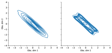
Figure 13: The kernel density estimated distribution of the “oscillating PCA 2” data for the model ‘TempVAE no dropout’. On the left we see the ‘TempVAE no dropout’ model and on the right the historical data.

B.7 Encoder Dependency

In this section, we we compare the ‘TempVAE’ model with ‘TempVAE backwards’, a version where the encoder structure is not implemented as in (13)- (17), but with a backward RNN, given by

$$\left\{\hat{\boldsymbol{\mu}}_{t}^{z},\boldsymbol{\hat{\Sigma}}_{t}^{z}\right\} =MLP^{z}_{I}\left(\hat{h}_{t}^{z}\right)$$ (30)

$$\hat{h}_{t}^{z} =RNN_{I}^{z}\left(\hat{h}_{t-1}^{z},z_{t-1},\hat{h}_{t}^{\leftarrow}\right)$$ (31)

$$\hat{h}_{t}^{\leftarrow} =RNN_{I}^{z}\left(\hat{h}^{\leftarrow}_{t+1},r_{t+1}\right)$$ (32)

$$z_{t} \sim\mathcal{N}\left(\hat{\boldsymbol{\mu}}_{t}^{z},\boldsymbol{\hat{\Sigma}}_{t}^{z}\right).$$ (33)

This is in consensus with the dependency structure of the posterior $p_{\boldsymbol{\theta}}(Z|R)$, shown in (11).

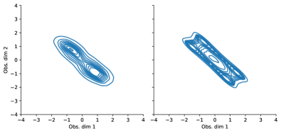
Figure 14: The kernel density estimated distribution of the “oscillating PCA 2” data for the model ‘TempVAE backwards’. On the left we see the ‘TempVAE backwards’ model and on the right the historical data.

Figure 14 displays the KDE estimation of the first two dimensions of the oscillating PCA data. In contrast to Figure 17, the plot for the model ‘TempVAE’ the structure is poorly fit.

Model	dax	noise	oscPCA2	oscPCA5	oscPCA10
TempVAE	20%	0%	20%	20%	20%
TempVAE backwards	10%	0%	10%	0%	0%

Table 9: The average count of active units given by (26) for the two models with different encoder architecture.

Table 9 shows that the auto-pruning is performing poorly when using only the backwards RNN for the model. As the encoding model is only an variational approximation to the actual posterior, we therefore decide to use the bidirectional architecture for our model.

C GARCH and DCC-GARCH

As benchmarks for the fit of the financial data, we consider three models.

1. GARCH: A GARCH(1,1) model, introduced by Bollerslev (1986).

2. DCC-GARCH-MVN: A Dynamic Conditional Correlation GARCH(1,1), introduced by Engle (2012), with a multivariate Gaussian distribution assumption for the error term.

3. DCC-GARCH-MVt: A Dynamic Conditional Correlation GARCH(1,1), with a multivariate t distribution assumption for the error term.

As the GARCH model is univariate, we model each dimension of our observed data separately. Therefore, we assume a correlation of 0 among the observed assets. The DCC-GARCH models can be seen a a multivariate extension of the first, where correlations are modeled as well. All models are linear and optimized by using Maximum Likelihood. We used the ‘rmgarch’ library in R (see Ghalanos (2019)).

D Activities on the Oscillating PCA Data Sets

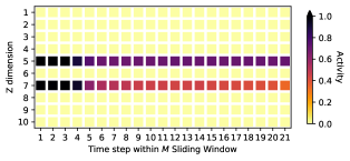
Figure 15: The activity statistics for the “oscillating PCA 5” data. We consider sequences of size $M=21$ as input. Depicted are the activity values of statistic (21) for the $\kappa=10$ dimensional latent space.

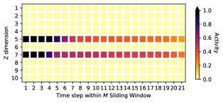
Figure 16: The activity statistics for the “oscillating PCA 10” data. We consider sequences of size $M=21$ as input. Depicted are the activity values of statistic (21) for the $\kappa=10$ dimensional latent space.

For “oscillating PCA 5” and “oscillating PCA 10”, the model identifies two active dimensions through time as can be seen in Figures 15 and 16. In our point of view, this is not problematic, since the non-linearities of the artificial neural net can be the reason, that less dimensions are needed to model the data appropriately. This can be observed in Table 10. Comparable scores are achieved for the Score Portfolio NLL. Furthermore, this can also be observed when we look at the fit of the model. For an excerpt of the first two dimensions see Figures 17, 18 and 19.

Score	oscPCA2	oscPCA5	oscPCA10
TempVAE Portfolio NLL	-5.21	-5.77	-4.80

Table 10: The different fit scores for the model TempVAE on the “oscillating PCA” data sets. Comparable scores are achieved for the Score Portfolio NLL. The multivariate Scores are not comparable, as the structure of the data is not Gaussian.

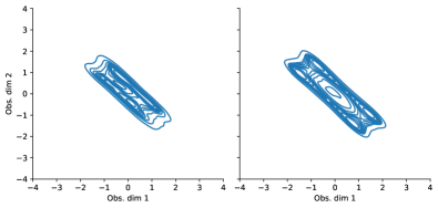
Figure 17: The kernel density estimated distribution of the first two dimensions $R_{t,1:2}$ of the “oscillating PCA 2” data. On the left we see the TempVAE model and on the right the historical data.

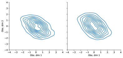
Figure 18: The kernel density estimated distribution of the first two dimensions $R_{t,1:2}$ of the “oscillating PCA 5” data. On the left we see the TempVAE model and on the right the historical data.

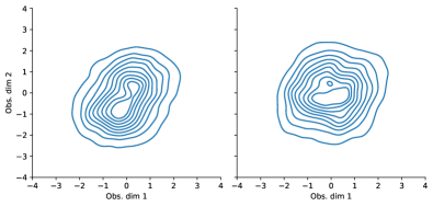
Figure 19: The kernel density estimated distribution of the first two dimensions $R_{t,1:2}$ of the “oscillating PCA 10” data. On the left we see the TempVAE model and on the right the historical data.

E Activities on the Stock Market Data and Model Adaptions for High-dimensional Data

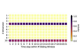
Figure 20: The activity statistics for the “Oscillating PCA 2” data. We consider sequences of size $M=21$ as input. Depicted are the activity values of statistic (21) for the $\kappa=10$ dimensional latent space.

In Figures 20 and 21, we see the activities for the 22 dimensional “DAX” data and the 397 dimensional “S&P500” data.

As the dimension of the data increased by a factor of 18 compared to the the other data sets in Section 4.1, we adjust the model implementation. For the RNN layers in (9), (14), (15), (16) we choose dimension 80, for the RNN layer in (6) we choose dimension 16. For the MLPs in (13), (5) and (8) we keep the two hidden layers and choose dimensions 60 and 30 for the first and second layer respectively. Furthermore do we reduce the initial learning rate to 1e-4 and change the $\beta$-annealing steps from 20 to 100.

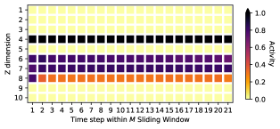
Figure 21: The activity statistics for the “S&P500” data. We consider sequences of size $M=21$ as input. Depicted are the activity values of statistic (21) for the $\kappa=10$ dimensional latent space.

F VaR and Scatterplots

In this section we will show some further VaR path plots for the models TempVAE, HS and DCC-GARCH-MVN. For this see Figures 22, 23 and 24.

Furthermore, we provide Scatterplots for thefirst two dimensions of the different models used for the VaR estimation in the figures 25, 26, 27 and 28.

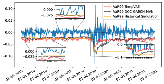
Figure 22: The VaR99 estimates for the models TempVAE, DCC-GARCH-MVN and HS on a fraction of the test data.

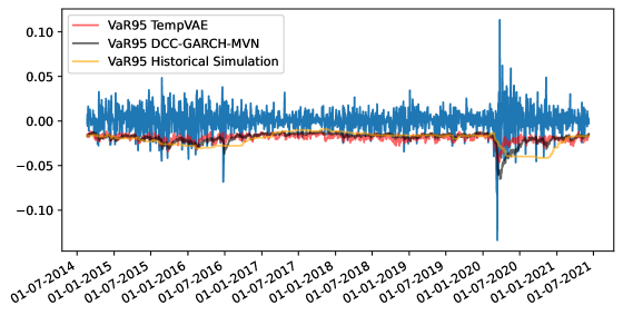
Figure 23: The VaR95 estimates for the two models TempVAE, DCC-GARCH-MVN and HS on the whole test data.

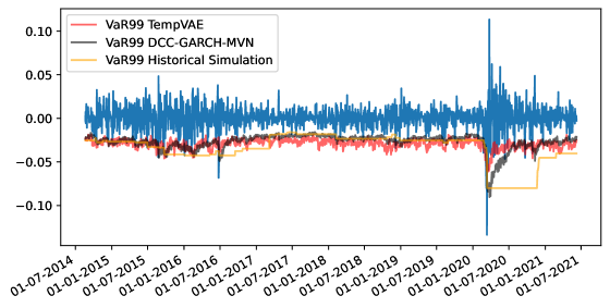
Figure 24: The VaR99 estimates for the two models TempVAE, DCC-GARCH-MVN and HS on the wohle test data.

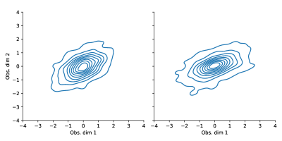
Figure 25: The kernel density estimated distribution of the first two dimensions $R_{t,1:2}$ of the “DAX” data. On the left we see the TempVAE model and on the right the historical data.

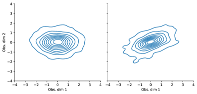
Figure 26: The kernel density estimated distribution of the first two dimensions $R_{t,1:2}$ of the “DAX” data. On the left we see the GARCH model and on the right the historical data.

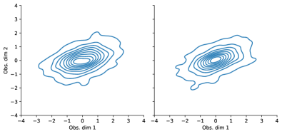
Figure 27: The kernel density estimated distribution of the first two dimensions $R_{t,1:2}$ of the “DAX” data. On the left we see the DCC-GARCH-MVN model and on the right the historical data.

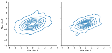
Figure 28: The kernel density estimated distribution of the first two dimensions $R_{t,1:2}$ of the “DAX” data. On the left we see the DCC-GARCH-MVt model and on the right the historical data.

References

- Arian et al. (2020) Hamidreza Arian, Mehrdad Moghimi, Ehsan Tabatabaei, and Shiva Zamani. Encoded Value-at-Risk: A Predictive Machine for Financial Risk Management. nov 2020. URL http://arxiv.org/abs/2011.06742.
- Arimond et al. (2020) Alexander Arimond, Damian Borth, Andreas G. F. Hoepner, Michael Klawunn, and Stefan Weisheit. Neural Networks and Value at Risk. SSRN Electronic Journal, 2020. ISSN 1556-5068. doi: 10.2139/ssrn.3591996.
- Bayer and Osendorfer (2014) Justin Bayer and Christian Osendorfer. Learning Stochastic Recurrent Networks. nov 2014. URL https://arxiv.org/abs/1411.7610v3.
- Bollerslev (1986) Tim Bollerslev. Generalized Autoregressive Conditional Heteroskedasticity. Journal of Econometrics, 31:307–327, 1986. ISSN 00954918.
- Bowman et al. (2015) Samuel R. Bowman, Luke Vilnis, Oriol Vinyals, Andrew M. Dai, Rafal Jozefowicz, and Samy Bengio. Generating Sentences from a Continuous Space. In CoNLL 2016 - 20th SIGNLL Conference on Computational Natural Language Learning, Proceedings, pages 10–21. Association for Computational Linguistics (ACL), nov 2015. URL http://arxiv.org/abs/1511.06349.
- Burda et al. (2016) Yuri Burda, Roger Grosse, and Ruslan Salakhutdinov. Importance Weighted Autoencoders. In 4th International Conference on Learning Representations, ICLR 2016 - Conference Track Proceedings. International Conference on Learning Representations, ICLR, sep 2016. URL http://arxiv.org/abs/1509.00519.
- Chen et al. (2020) Luyang Chen, Markus Pelger, and Jason Zhu. Deep Learning in Asset Pricing. sep 2020. URL https://papers.ssrn.com/abstract=3350138.
- Chen et al. (2009) Xiaoliang Chen, Kin Keung Lai, and Jerome Yen. A statistical neural network approach for value-at-risk analysis. Proceedings of the 2009 International Joint Conference on Computational Sciences and Optimization, CSO 2009, 2(71473155):17–21, 2009. doi: 10.1109/CSO.2009.350.
- Cho et al. (2014) Kyunghyun Cho, Bart Van Merriënboer, Caglar Gulcehre, Dzmitry Bahdanau, Fethi Bougares, Holger Schwenk, and Yoshua Bengio. Learning Phrase Representations using RNN Encoder-Decoder for Statistical Machine Translation. In EMNLP 2014 - 2014 Conference on Empirical Methods in Natural Language Processing, pages 1724–1734. Association for Computational Linguistics (ACL), jun 2014. ISBN 9781937284961. doi: 10.3115/v1/d14-1179. URL https://arxiv.org/abs/1406.1078v3.
- Chung et al. (2015) Junyoung Chung, Kyle Kastner, Laurent Dinh, Kratarth Goel, Aaron C. Courville, and Yoshua Bengio. A Recurrent Latent Variable Model for Sequential Data. In Advances in Neural Information Processing Systems, volume 28, pages 2980–2988. Neural information processing systems foundation, jun 2015. URL http://www.github.com/jych/nips2015{_}vrnnhttp://arxiv.org/abs/1506.02216.
- Engle (2012) Robert Engle. Dynamic Conditional Correlation. Journal of Business & Economic Statistics, 20(3):339–350, 2012. ISSN 07350015. doi: 10.1198/073500102288618487. URL https://www.jstor.org/stable/1392121.
- Fraccaro et al. (2016) Marco Fraccaro, Søren Kaae Sønderby, Ulrich Paquet, and Ole Winther. Sequential Neural Models with Stochastic Layers. In Advances in Neural Information Processing Systems, pages 2207–2215. Neural information processing systems foundation, may 2016. URL https://arxiv.org/abs/1605.07571v2.
- Fraccaro et al. (2017) Marco Fraccaro, Simon Kamronn, Ulrich Paquet, and Ole Winther. A Disentangled Recognition and Nonlinear Dynamics Model for Unsupervised Learning. In Advances in Neural Information Processing Systems, pages 3602–3611. Neural information processing systems foundation, oct 2017. URL https://arxiv.org/abs/1710.05741v2.
- Ghalanos (2019) Alexios Ghalanos. rmgarch: Multivariate GARCH models, 2019. URL https://cran.r-project.org/web/packages/rmgarch/citation.html.
- Goyal et al. (2017) Anirudh Goyal, Alessandro Sordoni, Marc-Alexandre Côté, Nan Rosemary Ke, and Yoshua Bengio. Z-Forcing: Training Stochastic Recurrent Networks. In Advances in Neural Information Processing Systems, volume 2017-Decem, pages 6714–6724. Neural information processing systems foundation, nov 2017. URL https://arxiv.org/abs/1711.05411v2.
- He et al. (2015) Kaiming He, Xiangyu Zhang, Shaoqing Ren, and Jian Sun. Delving Deep into Rectifiers: Surpassing Human-Level Performance on ImageNet Classification. In The IEEE International Conference on Computer Vision (ICCV), 2015. URL https://www.cv-foundation.org/openaccess/content{_}iccv{_}2015/html/He{_}Delving{_}Deep{_}into{_}ICCV{_}2015{_}paper.html.
- Kingma and Ba (2015) Diederik P. Kingma and Jimmy Lei Ba. Adam: A method for stochastic optimization. In 3rd International Conference on Learning Representations, ICLR, 2015.
- Kingma and Welling (2014) Diederik P. Kingma and Max Welling. Auto-Encoding Variational Bayes. In 2nd International Conference on Learning Representations, ICLR, 2014. URL https://arxiv.org/pdf/1312.6114.pdf.
- Kingma et al. (2014) Diederik P Kingma, Danilo J Rezende, Shakir Mohamed, and Max Welling. Semi-supervised Learning with Deep Generative Models. Technical report, 2014. URL http://arxiv.org/abs/1406.5298.
- Krishnan et al. (2017) Rahul Krishnan, Uri Shalit, and David Sontag. Structured Inference Networks for Nonlinear State Space Models. Proceedings of the AAAI Conference on Artificial Intelligence, 31(1), feb 2017. ISSN 2374-3468. URL https://ojs.aaai.org/index.php/AAAI/article/view/10779.
- Laloux et al. (2000) Laurent Laloux, Pierre Cizeau, Marc Potters, and Jean-Phillippe Bouchard. Random Matrix and Financial Correlations. International Journal of Theoretical and Applied Finance, 3(3):391–397, 2000.
- Liu (2005) Yan Liu. Value-at-Risk Model Combination Using Artificial Neural Networks. 2005.
- Luo et al. (2018) Rui Luo, Weinan Zhang, Xiaojun Xu, and Jun Wang. A Neural Stochastic Volatility Model. In Proceedings of the AAAI Conference on Artificial Intelligence, volume 32, apr 2018. URL www.aaai.org.
- Rezende et al. (2014) Danilo Jimenez Rezende, Shakir Mohamed, and Daan Wierstra. Stochastic Backpropagation and Approximate Inference in Deep Generative Models. In Proceedings of the 31 st International Conference on Machine Learning, pages 1278–1286. PMLR, jun 2014. URL https://arxiv.org/pdf/1401.4082.pdfhttp://proceedings.mlr.press/v32/rezende14.html.
- Sarma et al. (2003) Mandira Sarma, Susan Thomas, and Ajay Shah. Selection of Value-at-Risk Models. Journal of Forecasting, (22):337–358, 2003.
- Sicks et al. (2021) Robert Sicks, Ralf Korn, and Stefanie Schwaar. A Generalised Linear Model Framework for -Variational Autoencoders based on Exponential Dispersion Families. Journal of Machine Learning Research, 22(233):1–41, 2021. ISSN 1533-7928. URL http://jmlr.org/papers/v22/21-0037.html.
- Xu and Chen (2021) Xiuqin Xu and Ying Chen. Deep Stochastic Volatility Model. feb 2021. URL http://arxiv.org/abs/2102.12658.