Charm physics with a tmQCD mixed action

Abstract

We report on our ongoing determination of the charm quark mass and the masses and decay constants of various charmed mesons, obtained within a mixed-action setup. We employ $N_{f}=2+1$ CLS ensembles combined with a Wilson twisted mass valence action that eliminates the leading $O(a)$ effects from our target observables. Alongside our preliminary results, we will discuss an exploration of GEVP techniques aimed at optimizing the precision in view of the extension of the computation to heavier quark masses. We study the chiral-continuum extrapolation of decay constants for charm quark observables and the renormalized charm quark mass.

1 Introduction

Lattice QCD (LQCD) simulations allow to quantitatively study the realm of flavour physics, one of the most promising sectors for the search of physics beyond the Standard Model (SM). In particular, processes involving heavy quarks are essential to achieve reliable estimates of SM parameters and to examine the compatibility between the theory predictions and the experimental measurements. Our main goal is to compute hadronic matrix elements in the charm sector necessary to the determination of quantities of phenomenological interest such as the CKM matrix elements, reaching precisions that allow to improve the state-of-the-art.
In order to achieve reliable estimates we have developed a setup that aims at controlling the systematic uncertainties in LQCD simulations involving charm quarks [1]. In particular, we exploit a mixed action approach where in the sea sector we employ CLS $N_{f}=2+1$ gauge ensembles [2, 3] with open boundary conditions in the time direction and four fine values of the lattice spacing.
In the valence sector we take advantage of a twisted mass action with $N_{f}=2+1+1$ flavours at full twist. This ensures automatic $O(a)$ improvement of the observables up to residual lattice artifacts arising from the sea light quark masses [5].
For charmed semileptonics results from a tmQCD mixed action we refers to [6].

We present an update from [4] for the quark mass and for meson masses and decay constants in the charm-quark sector, with a particular focus on the chiral-continuum extrapolations to the physical point.

2 Lattice setup

2.1 Sea sector

In this work we use the gauge configurations produced within the CLS initiative [2], whose ensembles adopt the tree-level improved Lüscher-Weisz gauge action [7]. On the fermionic sector the action involves a Wilson Dirac operator for $N_{f}=2+1$ flavours [8] with the inclusion of the Sheikholeslami-Wolhert term to achieve non-perturbative $O(a)$ improvement [11].

This work is performed with four values of the lattice spacing ranging from 0.087 fm down to 0.050 fm. In Table 1 we report the list of CLS $N_{f}=2+1$ ensembles we used. In particular these ensembles lie along an approximate line of constant trace of the bare quark mass matrix,

$$\tr(M_{q})=2m_{q,u}+m_{q,s}=\text{const},$$ (1)

where $m_{q,f}=m_{0,f}-m_{\text{cr}}$. In practice, deviations from $\tr(M_{q})=\text{const}$ have been observed to be large at the coarsest lattice spacing [10]. Therefore, in the approach to the physical point we redefine the chiral trajectory by imposing

$$\phi_{4}\equiv 8t_{0}\bigg{(}\frac{1}{2}m_{\pi}^{2}+m_{K}^{2}\bigg{)}=\phi_{4}^{\text{phys}}\qquad\phi_{2}=8t_{0}m_{\pi}^{2}.$$ (2)

where the gluonic quantity $t_{0}$ is defined from the Wilson flow [9]. The dependencies of the observables on light sea quark masses are parametrised by $\phi_{2}$.

To ensures that $\phi_{4}$ passes across the physical point it is essential to apply small mass corrections to the bare quark masses through a low order Taylor expansion, as explained in [10]. Given a generic derived observable $\mathcal{O}$, its derivative with respect to the sea quark mass is given by

$$\derivative{\langle\mathcal{O}\rangle}{m_{q,i}}=\bigg{\langle}\partialderivative{\mathcal{O}}{m_{q,i}}\bigg{\rangle}-\bigg{\langle}\mathcal{O}\partialderivative{S}{m_{q,i}}\bigg{\rangle}+\langle\mathcal{O}\rangle\bigg{\langle}\partialderivative{S}{m_{q,i}}\bigg{\rangle},\qquad\quad\langle\mathcal{O}\rangle\rightarrow\langle\mathcal{O}\rangle+\sum_{i=1}^{N_{f}}\Delta m_{q,i}\derivative{\langle\mathcal{O}\rangle}{m_{q,i}},$$ (3)

where $S$ is the action. The shift of the observable depending on sea quark flavours is then given by right-most expression in the above equation, where the value of $\Delta m_{q,i}$ is obtained on each ensemble with an iterative procedure that matches $\phi_{4}$ to its physical value. The value of $\Delta m_{q,i}$ is chosen to be the same for all quark flavours.

Id	$\beta$	$N_{s}$	$N_{t}$	$m_{\pi}$ [MeV]	$m_{K}$ [MeV]	$M_{\pi}L$
H101	3.4	32	96	420	420	5.8
H102	3.4	32	96	350	440	5.9
H400	3.46	32	96	420	420	5.2
N200	3.55	48	128	280	460	4.4
N202	3.55	48	128	420	420	6.5
N203	3.55	48	128	340	440	5.4
N300	3.70	48	128	420	420	5.1
J303	3.70	64	196	260	470	4.1

Table 1: List of CLS $N_{f}=2+1$ ensembles used in the present study [2]. $N_{s}$ and $N_{t}$ refer to the spatial and temporal extent of the lattice. Approximate values of the pion and kaon masses are provided.

2.2 Valence sector

The mixed action setup employs in the valence sector a Wilson twisted mass Dirac operator [12] with $N_{f}=2+1+1$ valence flavours. This chiral rotation of the fields yields to an action in the twisted basis. In addition, we include a clover term and we use the non-perturbative determination of the Sheikholeslami-Wohlert coefficient for $N_{f}=3$ [13],

$$D_{\text{tm}}=\frac{1}{2}\sum_{\mu=0}^{3}\big{[}\gamma_{\mu}(\nabla^{*}_{\mu}+\nabla_{\mu})-a\nabla^{*}_{\mu}\nabla_{\mu}\big{]}+\frac{i}{4}ac_{\rm{\scriptscriptstyle SW}}\sum_{\mu,\nu=0}^{3}\sigma_{\mu\nu}\hat{F}_{\mu\nu}+\mathbf{m}_{0}+i\gamma^{5}\boldsymbol{\mu}_{0},$$ (4)

where $\nabla_{\mu}$ and $\nabla_{\mu}^{*}$ are the forward and backward covariant derivatives. The maximal twist regime is achieved by imposing the bare standard mass matrix to be equal to the critical mass $\mathbf{m_{0}}=\mathbb{1}\mathbf{m_{cr}}$. In this setup the twisted mass matrix $\boldsymbol{\mu}_{0}=\text{diag}(+\mu_{0,l},-\mu_{0,l},-\mu_{0,s},+\mu_{0,c})$ is associated to the physical bare quark masses.

In order to set the bare quark mass $\boldsymbol{m}_{0}$ to its critical value we tuned the valence PCAC quark mass to vanish in the light sector. This condition guarantees the full twist regime.

To recover the unitarity of the theory we perform the matching between sea and valence quark masses by imposing that the light pseudoscalar masses are equal in both sectors. More details on the matching procedure can be found in [14] and in the recent update [15].

In our simulations the charm quark is partially quenched, hence the matching procedure for the charm sector requires a different strategy. To tackle the issue we simulate at three different values of the charm twisted mass $\mu_{c}$ and we follow two different paths to tune the physical charm quark mass: we either employ the flavour averaged $D$ meson mass $m_{\bar{D}}=2/3m_{D}+1/3m_{D_{s}}$ or the charmonium $\eta_{c}$ effective mass, neglecting the disconnected contributions. The interpolation to physical values is performed jointly with a chiral-continuum extrapolations, as discussed in section 4.

3 Observables

The open boundary conditions in the Euclidean time direction modify the spectrum of the theory in the neighbourhood of the boundaries. In order to address the boundary effects, the sources of the two-point functions are set in the bulk, precisely in the middle of the lattice at $y_{0}=T/2$. The two-point functions are then given by

$$f_{P}(x_{0},y_{0})=a^{6}\sum_{\vec{x},\vec{y}}\langle P(x)P(y)\rangle\qquad f_{A_{\mu}}(x_{0},y_{0})=a^{6}\sum_{\vec{x},\vec{y}}\langle A_{\mu}(x)P(y)\rangle,$$ (5)

where $P$ and $A_{\mu}$ are the pseudoscalar density and the the improved axial current, respectively:

$$P(x)=\bar{\psi}(x)\gamma_{5}\psi(x)\qquad A_{\mu}(x)=\bar{\psi}(x)\gamma_{\mu}\gamma_{5}\psi(x)+ac_{A}\partial_{\mu}P(x).$$ (6)

In this work we rely on the generalized eigenvalue problem (GEVP) variational method to compute the spectrum and matrix elements of charmed mesons [16]. The basic idea behind the method is to consider a matrix of correlators $C(t)$ and solve the associated GEVP problem

$$C(t)v_{n}(t,t_{0})=\lambda_{n}(t,t_{0})C(t_{0})v_{n}(t,t_{0})\qquad n=1,\ldots,N,\quad t>t_{0},$$ (7)

where $N$ is the correlators matrix dimension.

We choose to avoid mixing of parity-odd and parity-even operators in a unique GEVP system to properly isolate the ground states. Having this in mind, we solve Eq. (7) for the two matrices of correlators

$$C_{PP}(t)=\bigg{[}\begin{matrix}\langle P(t)P(0)\rangle&\langle P(t+\tau)P(0)\rangle\\ \langle P(t)P(-\tau)\rangle&\langle P(t+\tau)P(-\tau)\rangle\end{matrix}\bigg{]}\qquad C_{VV}(t)=\bigg{[}\begin{matrix}\langle A_{k}(t)A_{k}(0)\rangle&\langle A_{k}(t+\tau)A_{k}(0)\rangle\\ \langle A_{k}(t)A_{k}(-\tau)\rangle&\langle A_{k}(t+\tau)A_{k}(-\tau)\rangle\end{matrix}\bigg{]}$$ (8)

where $C_{PP}(t)$ and $C_{VV}(t)$ denote the pseudoscalar and vector matrix of correlators, respectively. We tested several values of $\tau$, the time shift of the correlators, and we observed a mild dependence of the final results for small value of $\tau$. In what follows we set $\tau=3$.

Once the GEVP is solved, we extract the energy spectrum via [16]

$$E_{n}^{\text{eff}}=\log(\frac{\lambda_{n}(t,t_{0},\tau)}{\lambda_{n}(t+a,t_{0},\tau)})=E_{n}+p_{1}e^{-(E_{N+1}-E_{n})t},$$ (9)

where $E_{N+1}$ is the first unresolved excited state. The last term of the above equation is then used as a functional form to fit the effective energies, as described in detail in [16]. This allows to properly assess the systematic contribution from excited states and eventually we define the plateau region by imposing the statistical error to be four times larger than the systematic one.
In Fig. 1 we show the effective masses as extracted from the GEVP for two observables of interest in a representative ensemble. The same procedure is applied analogously to the extraction of the matrix elements from the generalised eigenvectors.

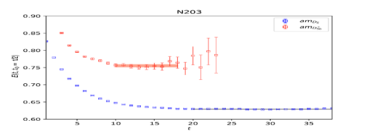
(a) Pseudoscalar spectrum in the charm-light sector

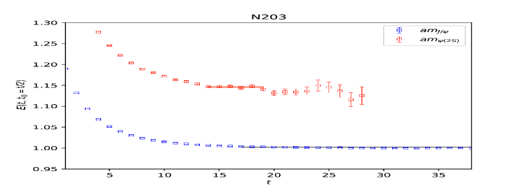
(b) Vector spectrum in the charmonium sector

Figure 1: Meson masses of the ground state and first excited state as extracted from the GEVP. The shaded bands show the plateau regions as determined by the procedure explained in the text.

4 Chiral-continuum extrapolations

After having determined the decay constants, the meson spectrum and the renormalized charm quark mass from every gauge ensemble listed in Tab. 1, we can finally go ahead with a combined chiral-continuum extrapolation, essential to obtain observables at the physical point. The latter is defined by $\phi_{2}=\phi_{2}^{\text{phys}}$ and $\phi_{H}=\phi_{H}^{\text{phys}}$ at zero lattice spacing, where

$$\phi_{2}=8t_{0}m_{\pi}^{2}\qquad\phi_{H}=\sqrt{8t_{0}}m_{H}\qquad m_{H}=m_{\bar{D}},m_{\eta_{c}}$$ (10)

are used to monitor the approach to the physical value of the bare light quark and the bare charm quark masses, respectively. Here $m_{H}$ labels the ground state of a charmed meson used to fix the charm quark mass, and we either employ the flavour averaged $D$ meson mass or the charmonium $\eta_{c}$ mass.

For the lattice spacing dependence of the observables we assume the leading cutoff effects to be of $O(a^{2})$ as the mixed action at full twist ensures the absence of $O(a)$ cutoff effects and the relevant $O(a)$ improved renormalization constant are know non-perturbatively from [17]. Eventually our general ansatz for the lattice spacing dependence is parametrised by

$$c_{\mathcal{O}}(\phi_{2},\phi_{H},a)=\frac{a^{2}}{8t_{0}}\big{(}c_{1}+c_{2}\phi_{2}+c_{3}\phi_{H}^{2}\big{)}+\frac{a^{4}}{(8t_{0})^{2}}\big{(}c_{4}+c_{5}\phi_{H}^{4}\big{)}.$$ (11)

Here we allow for cutoff terms describing the higher $O(a^{4})$ effects and we also consider cutoff effects proportional to the light quark masses. In the twisted mass formulation of LQCD at maximal twist, all the odd powers of the lattice spacing are suppressed.

For the continuum mass dependence of the observables of interest we employ the functional form

$$\sqrt{8t_{0}}\mathcal{O}^{\text{cont}}(\phi_{2},\phi_{H},0)=p_{0}+p_{1}\phi_{2}+p_{2}\phi_{H}.$$ (12)

We stress out that the light quark mass dependence is dominated by the sea pion mass $\phi_{2}$ only, since the mass shift corrections to the chiral trajectory ensure the kaon masses to be fixed by the condition $\tr(M_{q}^{R})=\text{const}$ as explained in Sec. 2.1. More sophisticated ansätze, e.g. including chiral logarithms, will be studied as more ensembles are incorporated.

Finally to arrive at a combined model we follow a similar strategy as proposed in [18] by either adding linearly or multiplying non-linearly Eqs. 11 and 12:

$$\begin{split}\sqrt{8t_{0}}\mathcal{O}^{\text{linear}}(\phi_{2},\phi_{H},a)&=\sqrt{8t_{0}}\mathcal{O}^{\text{cont}}(\phi_{2},\phi_{H},0)+c_{\mathcal{O}}(\phi_{2},\phi_{H},a),\\ \sqrt{8t_{0}}\mathcal{O}^{\text{non-lin}}(\phi_{2},\phi_{H},a)&=\sqrt{8t_{0}}\mathcal{O}^{\text{cont}}(\phi_{2},\phi_{H},0)\big{(}1+c_{\mathcal{O}}(\phi_{2},\phi_{H},a)\big{)}.\end{split}$$ (13)

Then, by considering all the possible combinations of the coefficients $c_{i}$ in Eq. (11), we end up with 64 different fit models. Since we are dealing with highly correlated data the uncorrelated $\chi^{2}$ does not yield reliable estimates of the fit paramaters. In practice we bypass this problem by employing the so-called $\chi^{2}$ expected, $\chi^{2}_{\text{exp}}$, as estimator for the goodness of a fit [19].

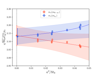
(a) Lattice spacing dependence of the renormalised charm quark mass for two representative model categories. The red points represent the charm quark mass fixed with the flavour average $m_{\bar{D}}$, while the blue points show results for the $\eta_{c}$ mass matching procedure.

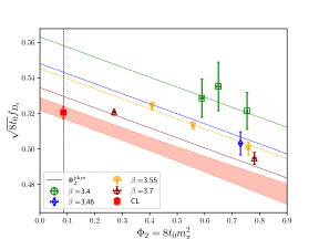
(b) Pion mass dependence of charm-strange decay
constant $f_{D_{s}}$ for a representative category.

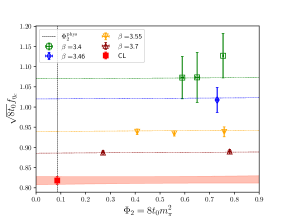
(c) Pion mass dependence of charmonium decay
constant $f_{\eta_{c}}$ for a representative category.

Figure 2: Comparison and examples of some of the best fits according to the AIC procedure. The two-dimensional representations are obtained by projecting to their physical values all the dependencies other than the ones showed in the plots. The shaded bands in the plots at the bottom show the continuum limit results.

In order to estimate the systematic effects arising from the model selection, we further classify our data into four different categories: we fix the physical charm mass by either employing the flavour averaged $D$ meson mass or the charmonium ground state $m_{\eta_{c}}$ and we either include all the gauge configurations in Tab. 1 or exclude the ones with $\beta=3.4$ to analyze the impact of cutoff effects when removing the coarsest lattice spacing. Within each category we perform fits by taking into account all the possible models arising from Eq. (13). This results in a total of 256 models for each observable. In Fig. 2 we show examples of some of the best chiral-continuum extrapolations for different categories.

In order to classify the goodness of each fit in a given category we use the Akaike Information Criteria (AIC) in the same way as employed in [18]. To this purpose we introduce the AIC parameter as $\text{AIC}=(N-k)\frac{\chi^{2}}{\chi^{2}_{\text{exp}}}+2k$, where $N$ is the number of data points and $k$ the number of parameters in the fit function. Then we proceed with a model average within each category according to

$$\langle\mathcal{O}\rangle=\sum_{m=1}^{M}w_{m}\langle\mathcal{O}\rangle_{m}\qquad\text{where}\qquad w_{m}=\exp(-\frac{1}{2}\text{AIC}_{m})\quad\text{s.t.}\quad\sum_{m=1}^{M}w_{m}=1,$$ (14)

where $\mathcal{O}$ is a given observable, $M$ labels the number of fit models, while $w_{m}$ are the corresponding weights given by the AIC. As proposed in [18], we estimate the systematic error arising from the model selection via

$$\sigma_{\mathcal{O}}^{2}=\sum_{m=1}^{M}w_{m}\langle\mathcal{O}\rangle_{m}^{2}-\bigg{(}\sum_{m=1}^{M}w_{m}\langle\mathcal{O}\rangle_{m}\bigg{)}^{2}.$$ (15)

In Fig. 3 we report a graphical representation of the model average procedure.

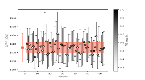
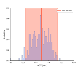
Figure 3: Summary of the model average procedure for the renormalised charm quark mass. Left: each circle labels the fit result for a given model in Eq. (13) for a representative category. The opacity of each circle is associated with the corresponding AIC weight in the model average. The filled box labels the model average as extracted according to Eq. (14). Right: histogram with fit results of each model in each category. In both plots the red shaded bands label the systematic error according to Eq. (15).

5 Preliminary results

In order to extract our preliminary results we choose the weighted average over the best results on all categories. We employ again Eq. (14), using as weights the inverse of the systematic and statistical errors added in quadrature. The final systematic error is estimated from the weighted standard deviation in Eq. (15). Following the chiral-continuum extrapolation analysis described in the previous section, we quote the ensuing results for charm quark observables in the $N_{f}=2+1$ theory. Here the first error is statistical and the second systematic.

• RGI charm quark mass: $\ M_{c}(N_{f}=3)=1514(13)(3)\ \text{MeV}$

• D-mesons decay constant: $\ f_{D}=209(3.5)(1.5)\ \text{MeV}\qquad f_{D_{s}}=242(4)(1)\ \text{MeV}$

• Charmonium decay constants: $\ f_{\eta_{c}}=392(8)(9)\ \text{MeV}\qquad f_{J/\Psi}=395(10)(4)\ \text{MeV}$

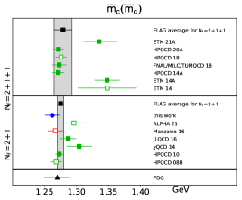
Figure 4: FLAG-style summary [20] of existing lattice results for the $\overline{\text{MS}}$-charm quark mass $\bar{m}_{c}(\bar{m}_{c})$ in GeV [21] (left) together with decay constants of the $D$ and $D_{s}$ mesons in MeV [22] (right). The blue circles label our results.

6 Conclusion and outlook

We have presented preliminary results from a tmQCD mixed-action setup at full twist for charm-light and charmonium decay constants and the RGI charm quark mass on a subset of CLS $N_{f}=2+1$ ensembles. In particular we highlight the usage of a GEVP variational method and an ongoing detailed analysis of the systematics in the chiral-continuum extrapolations. In order to improve the determination of charm-like observables a complete analysis including the most chiral and the finest CLS ensembles will be considered in the following stage of the project.

References

- [1] G. Herdoíza et al., EPJ Web Conf. 175 (2018), 13018 [arXiv:1711.06017 [hep-lat]].
- [2] M.Bruno et al., JHEP 1502 (2015) 043 [arXiv:1411.3982 [hep-lat]]
- [3] D. Mohler et al., EPJ Web Conf. 175 (2018) 02010 [arXiv:1712.04884 [hep-lat]]
- [4] J. Ugarrio et al. [Alpha], PoS LATTICE2018 (2018), 271 [arXiv:1812.05458 [hep-lat]].
- [5] A. Bussone et al. [ALPHA], PoS LATTICE2018 (2019), 270 [arXiv:1812.01474 [hep-lat]].
- [6] J. Frison et al., PoS LATTICE 2021 (2022), 320
- [7] M. Lüscher, P. Weisz, Commun. Math. Phys. 98, 433 (1985)
- [8] K.G. Wilson, Phys. Rev. D10, 2445 (1974)
- [9] M. Lüscher, JHEP 03 (2014) 092 [arXiv:1006.4518 [hep-lat]]
- [10] M. Bruno et al., Phys. Rev. D 95 (2017) no.7, 074504 [arXiv:1608.08900 [hep-lat]].
- [11] B. Sheikholeslami, R. Wohlert, Nucl. Phys. B259, 572 (1985)
- [12] R. Frezzotti et al.. (ALPHA), JHEP 08, 058 (1001). R. Frezzotti, G.C. Rossi, JHEP 10, 070 (2004). C. Pena et al., JHEP 09, 069 (2004)
- [13] J. Bulava, S. Schaefer, Nucl. Phys. B874, 188 (2013), 1304.7093
- [14] A. Bussone et al. [ALPHA], PoS LATTICE2018 (2019), 318 [arXiv:1903.00286 [hep-lat]].
- [15] G. Herdoíza et al., PoS LATTICE 2021 (2022), 258
- [16] M. Lüscher et al., Nucl. Phys. B339 (1990) 222-52. B. Blossier et al., JHEP 0904 (2009) 094
- [17] I. Campos et al., Eur. Phys. J. C. 78 (2018) 387, [arXiv:1802.05243 [hep-lat]]
- [18] J. Heitger et al., JHEP 2021 (2021) 288 [arXiv:2101.02694[hep-lat]]
- [19] M. Bruno, R. Sommer, In preparation. A. Ramos, PoS TOOLS2020 (2021), 045, ADerrors.jl
- [20] S. Aoki et al., "FLAG19" Eur. Phys. J. C. 80 (2020). See also "FLAG21" to appear.
- [21] I. Allison et al, Phys. Rev. D78(2008) 054513 [HPQCD 08B]. C. McNeile et al., Phys. Rev D82 (2010) 034512 [HPQCD 10]. Y. Yi-Bo et al., Phys. Rev D92 (2015) 034517 [QCD 14]. K. Nakayamaet al., Phys. Rev D94 (2016) 054507 [JLQCD 16]. Y. Maezawa et al., Phys. Rev D94 (2016) 034507 [Maezawa 16]. N. Carrasco et al., Nucl. Phys. B887 (2014) 19-68 [ETM 14]. C. Alexandrou et al., Phys. Rev. D90 (2014) 074501 [ETM 14A]. B. Chakraborty et al., Phys. Rev. D91 (2015) 054508 [HPQCD 14A]. A. Bazavov et al., Phys. Rev. D98 (2018) 054517 [FNAL/MILC/TUMQCD18]. A. T. Lytle et al., Phys. Rev. D98 (2018) 014513 [HPQCD 18]. J. Heitger et al., JHEP 288 (2021) [ALPHA 21]. C. Alexandrou et al., 2104.13408 [hep-lat] (2021) [ETM 21A]. D. Hatton et al., Phys. Rev. D102 (2020) 054511 [HPQCD 20A]
- [22] B. Blossier et al., JHEP 0907 (2009) 043 [ETM 09]. P. Dimopoulos et al., JHEP 1201 (2012) 046 [ETM 11A]. N. Carrasco et al., JHEP 1403 (2014) 016 [ETM 13B]. J. Heitger et al., PoS LAT 2013 (2014) 475 [ALPHA 13B]. W. Chen et al., Phys. Lett. B736 (2014) 231-236 [TWQCD 14]. A. Bazavov et al., PoS LAT 2012 (2012) 159 [FNAL/MILC 12B]. B. Blossier et al., Phys. Rev. D98 (2018) 054506 [Blossier 18]. E. Follana et al., Phys. Rev. Lett. 100 (2008) 062002 [HPQCD/UKQCD 07]. C. T. H. Favies et al., Phys. Rev. D82 (2010) 114504 [HPQCD 10A]. Y. Namekawa et al., Phys. Rev. D84 (2011) 074505 [PACS-CS 11]. A. Bazavov et al., Phys. Rev. D85 (2012) 114506 [FNAL/MILC 11]. H. Na et al., Phys. Rev. D86 (2012) 054510 [HPQCD 12A]. Y. Yi-Bo et al., Phys. Rev. D92 (2015) 034517 [QCD 14]. P. A. Boyle et al., JHEP 12 (2017) 008 [RBC/UKQCD 17]. A. Bazavov et al., PoS LAT 2012 (2012) 159 [FNAL/MILC 12B]. A. Bazavov et al., PoS LAT 2013 (2013) 405 [FNAL/MILC 13]. P. Dimopoulos et al., PoS LAT 2013 (2014) 314 [ETM 13F]. N. Carrasco et al., Phys. Rev. D91 (2015) 054507 [ETM 14E]. A. Bazavov et al., Phys. Rev. D90 (2014) 074509 [FNAL/MILC 14A]. A. Bazavov et al., Phys. Rev. D98 (2018) 074512 [FNAL/MILC 17]. Y. Chen et al., 2008.05208 [hep-lat] (2020) [QCD 20A]. R. Balasubramamian et al., Eur. Phys. J. C. 80 (2020) 412 [Balasubramamian 19]