Iterative saliency enhancement over superpixel similarity

Abstract

Saliency Object Detection (SOD) has several applications in image analysis. The methods have evolved from image-intrinsic to object-inspired (deep-learning-based) models. When a model fail, however, there is no alternative to enhance its saliency map. We fill this gap by introducing a hybrid approach, named Iterative Saliency Enhancement over Superpixel Similarity (ISESS), that iteratively generates enhanced saliency maps by executing two operations alternately: object-based superpixel segmentation and superpixel-based saliency estimation – cycling operations never exploited. ISESS estimates seeds for superpixel delineation from a given saliency map and defines superpixel queries in the foreground and background. A new saliency map results from color similarities between queries and superpixels at each iteration. The process repeats and, after a given number of iterations, the generated saliency maps are combined into one by cellular automata. Finally, the resulting map is merged with the initial one by the maximum bewteen their average values per superpixel. We demonstrate that our hybrid model can consistently outperform three state-of-the-art deep-learning-based methods on five image datasets.

1 Introduction

Saliency Object Detection (SOD) aims to identify the most visually relevant regions within an image. SOD methods have been used in an extensive range of tasks, such as image segmentation (Iqbal et al., 2020), compression (Wang et al., 2021a), quality assessment (Liu and Heynderickx, 2012), and content-based image retrieval (Al-Azawi, 2021).

Traditional SOD methods can combine heuristics to model object-inspired (top-down) and image-intrinsic (bottom-up) information. Object-inspired models expect that salient objects satisfy specific priors based on domain knowledge – e.g., salient objects in natural images are expected to be centered (Cheng et al., 2014), focused (Jiang et al., 2013), or have vivid colors (Peng et al., 2016). Image-intrinsic models provide candidate background and foreground regions used as queries and expect that salient regions be more similar to the foreground than background queries (Yang et al., 2013; Wu et al., 2018). Thus, their results strongly rely on those preselected assumptions.

Recently, deep-learning-based SOD methods have replaced preselected assumptions with examples of salient objects from a given training set. Such object-inspired methods usually rely on the backbone of a Convolutional Neural Network (CNN) trained for image classification. However, there are network architectures that can be easily trained from scratch (Qin et al., 2020).

Deep SOD methods are among the most effective, but they may miss foreground parts with similar colors (see Figure 1). Such incomplete saliency maps drift away from the results humans expect and there is no alternative to improve saliency maps. Since CNNs are object-inspired models that do not explore image-intrinsic information, we fill that gap by proposing a hybrid model, named Iterative Saliency Enhancement over Superpixel Similarity (ISESS), which explores superpixels in multiple scales and color similarity.

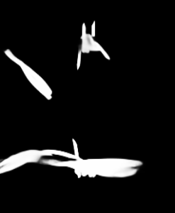
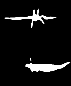
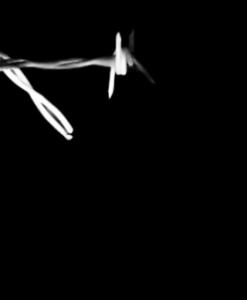
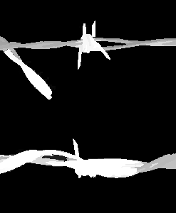
(a)	(b)	(c)	(d)

Figure 1: (a) Original image (top) and ground-truth segmentation (bottom). (b)-(d) BASNET (Qin et al., 2019) MSFNet (Zhang et al., 2021), and U²Net (Qin et al., 2020) saliency maps (top) and their enhanced maps (bottom) using the proposed approach.

ISESS can improve an input salience map over a few iterations of two alternate operations: object-based superpixel segmentation (”Belém et al., 2019) and superpixel-based saliency estimation. ISESS uses an input saliency map to estimate seeds for superpixel delineation and define superpixel queries in the foreground and background. A new saliency map is obtained by measuring color similarities between queries and superpixels, such that salient superpixels are expected to have high color similarity with at least one foreground query and low color similarity with most background queries. The process repeats for a given number of iterations, with a decreasing quantity of superpixels (increasing scale) per iteration. Although the process is meant to create progressively better saliency maps (Figure 2), we combine all output maps by cellular automata (Qin et al., 2015). By using the deep model as input, ISESS removes the need for preselected assumptions, providing an image-intrinsic extension of the provided object-inspired model. Finally, the image-intrinsic and initial (object-inspired) maps are merged by the maximum between their average values per superpixel, creating a hybrid saliency model. It is worth noting that ISESS does not depend on the choice of the object-inspired method.

(a)	(b)	(c)
(d)	(e)	(f)

Figure 2: ISESS saliency enhancement over multiple iterations. (a-c) original image, ground-truth segmentation and U²net saliency; (d-f) ISESS improvement over iterations 1, 3 and 10.

We demonstrate that our hybrid model consistently can outperform three state-of-the-art deep SOD methods (namely Basnet (Qin et al., 2019), U²Net (Qin et al., 2020), and Auto-MSFNet(Zhang et al., 2021)) using five well-known datasets. These results are confirmed by several metrics in all datasets, especially when images have multiple salient objects. Qualitative analysis also shows considerably enhanced maps whenever deep models fail to capture salient regions.

Therefore, the contributions of this paper are:

• A hybrid model for saliency object detection that does not rely on preselected assumptions while using object-inspired and multiscale image-intrinsic information.

• A first method to enhance object saliency maps, even when they are generated by deep-learning-based methods, with no need to combine multiple SOD methods (Section 2.2).

• A novel strategy that alternates over time object-based superpixel segmentation and superpixel-based saliency estimation (cycling operations never exploited) for saliency estimation.

Section 2 presents related work and ISESS is detailed in Section 3. Experiments with in-depth analysis of their results are presented in Section 4. We state conclusions and discuss future work in Section 5.

2 Related Work

2.1 Traditional SOD methods

2.1.1 Overview

Traditional SOD methods often rely on hand-crafted heuristics to model a set of characteristics shared by visually salient objects. These methods explore a combination of top-down object-inspired information — characteristics inherent to the object, not its relationship to other image regions — or bottom-up image-intrinsic strategies that use intrinsic image features to estimate saliency based on region similarity. Common top-down approaches expect salient objects centralized (Cheng et al., 2014), composed of vivid colors (Peng et al., 2016) or focused (Jiang et al., 2013). Early bottom-up strategies include modeling saliency according to pixel-level similarity to the mean image color (Achanta et al., 2009) or defining a global contrast by comparing all possible pairs of image patches (Cheng et al., 2014). Later, saliency estimators started using superpixels for better region representation, consistently outperforming pixel and patch-based methods. Most superpixel-based SOD methods use different heuristics to assemble a combination of top-down and bottom-up approaches.

2.1.2 Image-intrinsic superpixel-based approaches

Apart from superpixel similarity methods that use global contrast (Jiang et al., 2013), bottom-up approaches (image-intrinsic) require a strategy to select superpixels that represent candidate foreground and background regions — namely, queries. The three commonest query selection strategies are based on sparsity, backgroundness, or objectness. Methods based on low-rank (LR) matrix recovery (Lang et al., 2011; Peng et al., 2016) use sparsity, and assume an image can be divided into a highly redundant background-likely low-rank matrix and a salient sparse sensory matrix. Superpixel-graph-based methods (Zhu et al., 2014; Zhang et al., 2018a; Yang et al., 2013; Wu et al., 2018) estimate saliency by combining superpixel-adjacency contrast with the similarity between every superpixel and probable background and foreground queries. Background queries are usually defined at the image borders, but the methods propose strategies to mitigate error when this assumption is invalid. Such strategies include estimating four saliency maps (one for each image border) so that regions consistently highlighted are taken as salient (Yang et al., 2013); using only border regions that share common characteristics amongst themselves (Wu et al., 2018); include a weight function for the query regions, so that superpixels that grow close to the image center have a lower weight than the ones connected to the image limits (Zhu et al., 2014). However, background-based saliency methods often highlight parts of the desired object even when using those error-mitigating strategies. To improve upon background-based saliency, one can use background saliency to define salient regions as foreground queries and then compute a foreground saliency score (Yang et al., 2013; Wu et al., 2018).

A major drawback in all methods above is their reliance on heuristics or domain-specific prior information. We combine saliency estimations from a given object-inspired deep SOD model and the proposed superpixel-based image-intrinsic model to avoid the heuristic-based approach. Additionally, the proposed method implements a novel enhancement loop that iteratively improves object representation by alternating executions of object-based superpixel segmentation and saliency estimation. The iterative aspect of our method explores multiple superpixel scales, which allows us to not impose spatial constraints as superpixel-graph-based methods do. We simply compute feature similarity between all superpixels and queries, leaving the pixel adjacency relationship to be handled by the different superpixel segmentations.

2.2 Saliency map improvement by aggregation

Multiple SOD methods have been combined to improve incomplete saliency maps Qin et al. (2015); Chen et al. (2018); Singh and Kumar (2020); Li et al. (2018a). Unsupervised methods may use min-max operations over the estimated foreground and background regions Singh and Kumar (2020), Baysian Frameworks for iteratively enhancing consistently salient regions over time (Qin et al., 2015), or DS evidence theory to learn weights for the multiple saliency maps in a fusion framework (Chen et al., 2018). Supervised methods often learn regressors that combine multiple saliency maps into a single saliency score using bootstrap learning Tong et al. (2015); Li et al. (2018a).

However, such aggregation strategies create a significant processing overhead due to the execution of multiple SOD methods, and their high precision depends on an agreement among most saliency maps with respect to the salient object. To our knowledge, our approach is the first that improves incomplete saliency maps without requiring aggregation of multiple SOD methods.

2.3 Deep-learning methods

2.3.1 Multi-layer perceptron (MLP)-based approaches

The usage of deep neural networks for saliency detection has been extensive in the past few years. As presented in a recent survey (Wang et al., 2021b), earlier attempts used MLP-based approaches (Zhang et al., 2016; He et al., 2015; Liu and Han, 2016), adapting networks trained for image classification by appending the feature-extraction layers to a pixel-patch classifier. Despite the improvement of these models over heuristic-based traditional methods, they were incapable of providing consistent high spatial accuracy, primarily due to relying on local patch information.

2.3.2 Fully-Convolutional Neural-Networks (FCNN)

FCNN-based methods improved object detection and delineation, becoming the most common network class for visual saliency estimation. Most FCNN models use the pretrained backbone of a CNN for image classification (e.g. DenseNet (Huang et al., 2017), VGG (Simonyan and Zisserman, 2014), and Resnet (He et al., 2016)) and a set of strategies to exploit the backbone features in the fully convolutional saliency model. These strategies often explore information from shallow and deep layers, providing methods for aggregating or improving the multiple-scale features. Some methods use multiple atrous convolutions with different sampling rates (Chen et al., 2014, 2017); Zhang et al. (Zhang et al., 2017) propose a generic framework that integrates multiple feature-scales into multiple resolutions; in (Zhang et al., 2018c), an attention-guided recurrent convolutional network is proposed to integrate multi-level features and reintroduce high-level semantic information from deep layers to shallow layers; Zhang et al. (Zhang et al., 2018b) presented a bi-direction module to pass information between the shallow and deep layers, and use a pyramid fusing strategy to combine multi-scale information.

The methods described above upsample directly from the low-resolution deep layers back to the full-size input layer, resulting in significant information loss. To reduce the negative impact of drastic upsampling, several methods have adopted the encoder-decoder structure to gradually re-scale the low-resolution features (Liu et al., 2019; Tang et al., 2018; Qin et al., 2020, 2019; Zhang et al., 2021). Each method proposes a different strategy to exploit the multi-scale features in the decoder. As examples, Liu et al. (Liu et al., 2019) propose a global guidance module based on pyramid pooling to explicitly deliver object-location information in all feature maps of the decoder; Tang et al. (Tang et al., 2018) proposed stacking U-shaped networks and densely connect their layers, providing a shared-memory implementation strategy to alleviate the memory-heavy requirements. In recent work, Miao et al. (Zhang et al., 2021) proposes the Auto- Multi-Scale Fusion Network (Auto-MSFNet), which uses Network Architecture Search (NAS) as inspiration to propose an automatic fusion framework instead of trying to elaborate complex human-described strategies for multi-scale fusion. They introduce a new search cell (FusionCell) that receives information from multi-scale features and uses an attention mechanism to select and fuse the most important information.

Boundary information can be used to achieve better object delineation. Early on, Luo et al. (Luo et al., 2017) proposed a new loss that heavily penalizes boundary regions for training an adaptation of VGG-16; Li et al. (Li et al., 2018b) proposes a two-step methodology that extracts contours from an input image and then extrapolates a saliency-map out of the contours; Su et al. (Su et al., 2019) proposes a three-stream methodology with a boundary location stream, an interior perception stream, and a boundary/region transition prediction; and Zhao et al. (Zhao et al., 2019) uses an encoder-decoder network to extract multi-scale salient-object features from a backbone, and uses both the high-resolution backbone features and the encoder-decoder object-location information to assist an edge-feature extraction that guides the delineation for the final saliency estimation. Instead of explicitly or exclusively using boundary information, Qin et al. (Qin et al., 2019) proposes the Boundary-Aware Segmentation Network (BASNET) with a hybrid loss to represent differences between the ground-truth and the predictions in a pixel, patch, and map level. The loss is a combination of the Binary-Cross-Entropy (pixel-level) (De Boer et al., 2005), the Multi-scale Structural Similarity (Wang et al., 2003) (patch-level), and the Intersection over Union (Máttyus et al., 2017) (map-level). Their strategy consists of a prediction module that outputs seven saliency maps (an upsampled output of each decoder layer) and a residual refinement module that outputs one saliency map at the final decoder layer. All output maps are used when computing the hybrid loss, and both modules are trained in parallel.

All earlier methods require a backbone pretrained in a large classification dataset and often require many training images for fine-tuning. Recently, Qin et al. (Qin et al., 2020) proposed a nested U-shaped network by the name of U²Net, that has achieved impressive results without requiring a pretrained backbone. Their approach consists of extracting and fusing multiple-scale information throughout all stages of the encoder-decoder by modeling each stage as a U-shaped network. By doing so, they can extract deep information during all network stages without significantly increasing the number of parameters (due to the downscaling inside each inner U-net).

Even though each presented method has specific characteristics and shortcomings, the main goal of this paper is to aggregate image-intrinsic information to the complex object-inspired models provided by the deep saliency methods. In this regard, we selected as baseline three state-of-the-art saliency estimators that apply different strategies to learn their models: U²Net (Qin et al., 2020), which has the novelty of not requiring a pre-trained backbone; BASNet (Qin et al., 2019), that provides a higher delineation precision due to its boundary-awareness; and Auto-MSFNet (Zhang et al., 2021), which uses a framework to learn the fusion strategies that humans commonly define.

3 Proposed approach: Iteractive Saliency Enhancement using Superpixel Similarity (ISESS)

ISESS aims to improve the results of complex deep-learning-based SOD models by adding image-intrinsic information. For such, ISESS combines alternate executions of object-based superpixel segmentation and superpixel-based saliency estimation. The multiple executions of both operations generate enhanced saliency maps for integration into a post-processed map, which is subsequently merged with the initial saliency map of the deep SOD model. Figure 3 illustrates the whole process, described in Sections 3.1 and 3.2.

Figure 3: A depiction of the proposed method. The saliency/superpixel enhancement loop is presented inside the Saliency Enhancement Module (SEM). Note that the SEM inside the Saliency Integration Module (SIM) runs only once. The red arrows represent a flow happening only on the first iteration.

3.1 Saliency Enhancement Module

The saliency enhancement module starts by computing a superpixel segmentation since ISESS is a superpixel-based saliency enhancer. For such, we use the Object-based Iterative Spanning Forest algorithm (OISF) (”Belém et al., 2019).

In short, OISF  represents an image as a graph, whose pixels are the nodes and the arcs connect 8-adjacent pixels, elects seed pixels based on an input object saliency map, and executes the Image Foresting Transform (IFT) algorithm (Falcão et al., 2004) followed by seed refinement multiple times to obtain a final superpixel segmentation. Each superpixel is then represented as an optimum-path tree rooted at its most closely connected seed.

For the initial seed sampling based on a saliency map, we use OSMOX (Belém et al., 2019), which allows user control over the ratio of seeds to be placed inside and outside the salient objects with no need to binarize the saliency map. For seed refinement, we set the new seed of each superpixel to be the closest pixel to its geometrical center.

For this setup of OISF, the user has to provide four parameters: $\alpha$ to control the importance of superpixel regularity; $\beta$ to control the importance of boundary adherence; $\gamma$ to provide a balance between saliency information and pixel colors; and $i_{o}$ the number of iterations to obtain a final superpixel segmentation. Within the method proposed in this paper, we fixed $\alpha=12$ and $\beta=0.5$ as suggested in  (Vargas-Muñoz et al., 2019), while $\gamma$ and $i_{o}$ were tuned by grid searching (see Section 4.1).

The only specific implementation change regarding the superpixel segmentation algorithm is the percentage of object seeds required by the seed sampler. Instead of fixing a percentage that would fit most images, we set the number of seeds inside salient areas to be $n_{os}=n_{s}*n_{c}$, where $n_{c}$ is the number of connected components found by Otsu binarization of the saliency map resultant from the last iteration, and $n_{s}$ is a parameter. This way, the number of superpixels depends on how many salient objects the oversegmentation is trying to represent.

Within this paper, let the saliency score of either a pixel or a superpixel be represented as $\textbf{s}(\cdot)$. At the end of each iteration, the saliency score of a superpixel is given by the previously computed pixel-wise saliency map and is taken as the mean saliency score of all pixels inside the superpixel. We do not reuse the saliency of a superpixel directly because the superpixel segmentation changes at each iteration.

Let $\mathcal{S}$ be a superset of all superpixels, $\textbf{F}:\mathcal{S}\rightarrow\mathbb{R}^{m}$ map to every superpixel the mean feature vector of all its pixels — in this paper, $m=3$ because we use the pixel colors in the CIELab color-space as features. We define two query lists, $\mathcal{Q}_{F}$ for foreground superpixels, and $\mathcal{Q}_{B}$ for background ones, where $\mathcal{Q}_{F}\cup\mathcal{Q}_{B}=\mathcal{S}$. Take $\psi$ to be the Otsu threshold of the previously computed saliency map, then, the query lists are defined as follows: $\textit{S}\in\mathcal{Q}_{F}\leftrightarrow\textbf{s}(\textit{S})\geq\psi$, and similarly, $\textit{S}\in\mathcal{Q}_{B}\leftrightarrow\textbf{s}(\textit{S})<\psi$.

Taking $\textit{S},\textit{R}\in\mathcal{S}$ as superpixels, we define a Gaussian-weighted similarity measure between superpixels as:

$$\textbf{sim}(\textit{S},\textit{R})=\exp^{\frac{-\textbf{d}(\textbf{F}(\textit{S}),\textbf{F}(\textit{R}))}{\sigma^{2}}},$$ (1)

where $\textbf{d}(\textbf{F}(\textit{S}),\textbf{F}(\textit{R}))$ is the euclidean distance between the superpixel’s mean features, and $\sigma^{2}=0.01$ is the variance used to regulate the dispersion of similarity values.

Using the similarity measure and the query lists, we define two saliency scores for each superpixel: one based on foreground queries, and the other on background ones. For the foreground saliency score, a region is deemed to be salient if it shares similar characteristics to at least one other foreground region:

$$\textbf{s}_{f}(\textit{S})=\max\limits_{\forall\textit{R}\in\mathbb{Q}_{F}}\{{\textbf{{sim}({S}, {R})}}\}$$ (2)

However, when $\textit{S}=\textit{S}_{f}\in\mathbb{Q}_{F}$ is a foreground query, its foreground saliency score equals one, which is an out-scaled value as compared to other gaussian-weighted similarities. To keep foreground queries with the highest score but in the same scale of the remaining superpixels’ scores, we update their values to match the highest non-foreground query region’s saliency: $\textbf{s}_{f}(\textit{S}_{f})=\max\limits_{\forall\textit{Q}\notin\mathcal{Q}_{F}}\{{\textbf{s}_{f}(\textit{Q})}\}$. By doing so, we allow for a forced exploration of possible foreground regions at each iteration.

Similarly, the background-updated saliency score defines that a superpixel is salient if it has low similarity to most background queries:

$$\textbf{s}_{b}(\textit{S})=1-\frac{\sum\limits_{\forall\textit{R}\in\mathbb{Q}_{B},\textit{S}\neq\textit{R}}{\textbf{sim({S}, {R})}}}{|\mathbb{Q}_{B}|}.$$ (3)

When the background is too complex, the normalized mean difference of all superpixels will be close to fifty percent, resulting in a mostly gray map with little aggregated information (Figure 4). To detect those scenarios, we compute a map-wise distance to fifty percent probability $d_{0.5}=\frac{1}{|\mathbb{S}|}\sum\limits_{\forall\textit{S}\in\mathbb{S}}{(\textbf{s}_{b}(\textit{S})-0.5)^{2}|\textit{S}|}$. For maps with $d_{0.5}<0.1$, we set the background saliency score to be the saliency of the previous iteration $\textbf{s}_{b}(\textit{S})=\textbf{s}^{i-1}(\textit{S})$, where $\textbf{s}^{i-1}$ is the final saliency computed in the last iteration and $\textbf{s}^{0}$ is the initial deep-learning saliency.

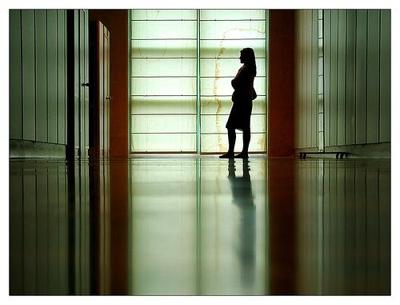
(a)	(b)
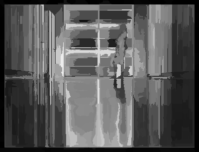
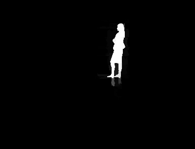
(c)	(d)

Figure 4: Background-based saliency with $d_{0.5}<0.1$ due to a complex background, resulting on a map with little relevant information. (a) original image; (b) U²Net map; (c) background-based saliency; (d) saliency used instead of (c).

The final saliency score for the iteration is the product of both saliencies:

$$\textbf{s}^{i}(\textit{S})=\textbf{s}_{f}(\textit{S})*\textbf{s}_{b}(\textit{S}).$$ (4)

By multiplying both scores, the combined saliency ignores any region that was hardly taken as non-salient by foreground or background saliency and keeps a high score for regions taken as salient in both maps. The new score is saved together with the superpixel representation used to create it. Then, the saliency is fed to the superpixel algorithm to restart the enhancement cycle. We reduce the number of superpixels by $20\%$ at each iteration to a minimum of $200$ superpixels.

The result of all iterations is then combined using the method described in Section 3.2

3.2 Saliency Integration Module

To integrate the saliency maps created throughout the iterations, we use a traditional unsupervised saliency integrator method (Qin et al., 2015) that models an update function using a Bayesian framework to iteratively update a Cellular Automata whose cells are derived from a stack of the saliency maps. Note that we are using saliency integration to combine the multiple outputs of our iterative approach, not aggregating different saliency methods.

In short, the saliency maps are stacked to form a three-dimensional grid where the (x,y) coordinates match the saliency map’s (x,y) coordinates and z is the direction in which the different maps are stacked. The pixels are then updated over it iterations in a way that the new pixel saliency depends on how consistently salient its adjacency is. The adjacency used is a cuboid adjacency $\mathbb{C}_{p}$ around the pixel $p$, so that a pixel $q$ is considered adjacent to a $p$ if $|(x_{p}-x_{q})|\leq 1,|(y_{p}-y_{q})|\leq 1$; i.e. a 4-adjacency extended to all maps on the z-axis.

For the update rule, the saliency score is represented as log odds: $\textbf{l}(p)=\frac{\textbf{s}(p)}{1-\textbf{s}(\textit{S})}$ so that the value can be updated by performing subsequent sums. The value changes according to the rule:

$$\textbf{s}^{t+1}(p)=\textbf{l}(p)+\sum\limits_{\forall q\in\mathbb{C}_{p}}{\lambda\delta(q)},$$ (5)

where $\lambda$ is a constant that regulates the update rate, and $\delta(\cdot)\in\{-1,1\}$ is a signal function that makes the saliency either increase or decrease at each update depending on whether $\textbf{s}(q)$ is greater or smaller than the Otsu threshold of the saliency map that originated the cell. Essentially, if a pixel is surrounded by more foreground than background regions, its saliency increase over time by a rate of $\lambda$; likewise, the saliency decreases for pixels in a non-salient adjacency.

Afterward, the integrated map is run through the last iteration of saliency estimation using Equation 2 and the initial number of superpixels, creating the last color-based saliency score $\textbf{s}_{c}$. This last estimation serves two purposes: improve object delineation by relying on the quality of the superpixel algorithm — rather than depending on the cuboid adjacency relation; and eliminate unwanted superpixel leakage that may occur when the superpixel number is reduced (Section 4.2.2).

Lastly, we reintroduce the deep object-inspired model by averaging its saliency values inside the superpixels of the last segmentation, which defines another saliency score for each superpixel:

$$\textbf{s}_{d}(\textit{S})=\frac{1}{|\textit{S}|}\sum\limits_{\forall p\in\textit{S}}{\textbf{s}_{0}(p)},$$ (6)

where $\textbf{s}_{0}(p)$ is the saliency score provided by the network. The final saliency score is than defined as:

$$\textbf{s}_{f}(p)=\max\{\textbf{s}_{d}(p),\textbf{s}^{i}(p)\}.$$ (7)

Therefore, the final saliency map will highlight salient regions according to the image-intrinsic or the superpixel-delineated object-inspired model.

4 Experiments and Results

4.1 Datasets and experimental setup

Datasets: We used five well-known datasets for comparison among SOD methods. DUT_OMRON is composed of 5168 images containing one or two complex foreground objects in a relatively cluttered background; HKU-IS contains 4447 images with one or multiple low contrast foreground objects each; ECSSD consists of 1000 images with mostly one large salient object per image in a complex background; ICoSeg consists of 643 images usually with several foreground objects each; and SED2 is formed by 100 images with two foreground objects per image.

Parameter tuning: The baselines networks were used as provided by the authors since they have been pretrained on datasets with similar images (e.g., DUT_OMRON). For ISESS, we randomly selected 50 images from each dataset, totalizing a training set with 300 images, to optimize its parameters by grid search. The remaining images compose the test sets of each dataset. Grid search was performed with saliency maps from each baseline, creating three sets of parameters (one per baseline). Most parameters were optimized to the same value independently of the baseline, except for the number of iterations $i$, the number of superpixels $n$, the number of foreground seeds per component $n_{s}$, and the number of OISF iterations $i_{o}$. Taking the order U²Net, BASNET, and MSFNet, the parameters were respectively, $i=\{12,9,12\}$, $n=\{2500,200,2500\}$, $n_{s}=\{10,30,30\}$, and $i_{o}=\{5,3,1\}$. The rest of the parameters with fixed values for all methods were optimized to be: $\gamma=10.0$, $\sigma^{2}=0.01$, $\lambda=0.0001$, $t=3$, where $\gamma$ is related to the superpixel segmentation algorithm, $\sigma^{2}$ is the gaussian variance for the graph node similarity, $\lambda$ and $t$ are related to the cuboid integration.

Evaluation metrics: We used six measures for quantitative assessment. (1) Mean Structural-measure, $S_{m}$, which evaluates the structural similarity between a saliency map and its ground-truth; (2) max F-measure, $\max F_{\beta}$, which represents a balanced evaluation of precision and recall for simple threshold segmentation of the saliency maps; (3) weighted F-measure, $F_{\beta}^{w}$, which is similar to $\max F_{\beta}$ but keeps most saliency nuances by not requiring a binary mask; (4) Mean Absolute Error, $MAE$, that provides a pixel-wise difference between the output map and expected segmentation; (5) mean Enhanced-alignment measure, $E_{\psi}^{m}$, used to evaluate local and global similarities simultaneously; and (6) precision-recall curves, which display precision-recall values between the expected segmentation and saliency maps binarized by varying thresholds.

Post processing: ISESS can sometimes score a superpixel with close-to-zero saliency values. These small saliencies are not visually perceived by the observer but can significantly impair the presented metrics (Figure 5). In the image presented, the bottom-left quadrants (with a little more than a fourth of the total image weight) had a superpixel slightly salient (a value below $2\%$ of the maximum saliency) by ISESS, which caused the local SSIM to change from a full match on the original map to a complete miss on the enhanced map. To deal with these small values, we eliminate regions in the map with saliency lower than half of the Otsu threshold.

(a)	(b)
(c)	(d)

Figure 5: Example of drastic $S_{m}$ difference between two similar saliency maps. (a) original image with ground-truth objects delineated in red; (b) BASNET saliency map divided into quadrants, with each quadrant weight and Structural Similarity values annotated; (c) same as (b) but with the map enhanced by ISESS; (d) histogram-manipulated (c) to show the detail that caused the large difference in similarity value.

4.2 Ablation study

To analyze the impact of some decisions within our proposal, we present ablation studies on (i) the effects of re-introducing the deep model at the end of the last iteration; (ii) re-using the initial number of superpixels at the last iteration. We used the same parameters as the ones reported in Section 4.1 for the ablation studies.

4.2.1 Ablation on reintroducing the deep saliency model

The goal of ISESS is to improve the complex and robust deep models by adding information more closely related to what a human observer expects. Not re-introducing the deep model would imply creating a color-based model that keeps all the robustness of the deep-learning ones, which is hardly feasible.

An example of why the proposed color-based model is often insufficient can be seen in Figure 6. The object of interest was less uniformly salient: The armband the player is wearing has significantly different colors than the rest of the object, which caused the model not to consider it as part of the foreground. In that example, ISESS mainly contributed to creating sharper edges.

(a)	(b)
(c)	(d)

Figure 6: Good example of the re-introduction of the deep-model saliency. (a) original image; (b) U²Net saliency map; (c-d) ISESS without and with the reintroduction of the deep model, respectively

The downside of re-introducing the deep model is that it reduces the influence of ISESS on wrongfully salient regions. Take Figure 7 as an example: The deep-model wrongfully highlighted part of the airplanes’ smoke trail; ISESS did perceive this to be a mistake and removed it entirely; the re-introduction of the deep-model also brought back the error. However, the smoke trail’s saliency was reduced thanks to combining the deep model with the superpixel segmentation.

(a)	(b)	(c)	(d)

Figure 7: Bad example of the re-introduction of the deep-model saliency. (a) original image; (b) U²Net saliency map; (c-d) ISESS without and with the reintroduction of the deep model, respectively

4.2.2 Ablation on using the initial number of superpixels for the last iteration

As the iterations progress and the number of superpixels decreases, the object-representation provided by the superpixels can worsen due to either leakage to the background or under-segmentation of too distinct object parts. As exemplified in Figure 8, the wings of the airplanes were lost in the final saliency map due to superpixel leakage. The model could adequately highlight most of the planes’ wings by increasing the number of superpixels at the last iteration.

(a)	(b)	(c)
(d)	(e)	(f)

Figure 8: Bad object representation due to the superpixel decrease. (a-c) original image and superpixel segmentation using the reduced and the full number of superpixels, respectively; (d-f) U²Net, U²Net+ISESS without and with the superpixel number increase at the last iteration, respectively. Note part of the object missing (pink circle) due to superpixel leakege.

4.3 Quantitative comparisons

Table 1 shows that the proposed method can consistently improve $maxF_{\beta}$, $F_{\beta}^{w}$, $MAE$ and $E_{\psi}^{m}$ for U²Net (Qin et al., 2020) and BASNET (Qin et al., 2019) in all five datasets, and achieve similar $S_{m}$. On both datasets composed mostly of images containing more than one object (Sed2 and ICoSeg), the results were even more expressive, indicating that ISESS can considerably improve the saliency representation of similar objects.

The precision-recall curves show a clear advantage of ISESS-enhanced maps over the non-enhanced ones on datasets mainly consisting of multiple objects (sed2, and icoseg). There is a breakpoint where ISESS loses precision more rapidly than non-enhanced maps on the other three datasets. We attribute the rapid precision loss to ISESS highlighting more parts of non-salient objects deemed partially salient by the deep models (Figure 9). By looking at the $maxF_{\beta}$, we see that by segmenting ISESS maps using an adequate threshold, the segmentation results are often better than the non-enhanced maps on almost every combination of method and dataset.

The better representation of non-salient objects discussed before also highly impacts the $S_{m}$. Similar to the example shown in Figure 5, spatially extending the saliency of a non-salient object to other image quadrants drastically affects the quality of the map according to the Mean Structural-measure.

Regarding Auto-MSFNet, apart from the ICoSeg and SED2, ISESS could not improve its metrics. By analyzing the precision-recall curves, we identified that Auto-MSFNet has the lowest precision of all three methods. We realized that the AutoMSF-Net creates more frequently partially salient regions on non-salient objects. Both examples used in Figure 9 were taken from the AutoMSF-Net results. Therefore, ISESS seems to over-trust the deep model on non-salient regions.

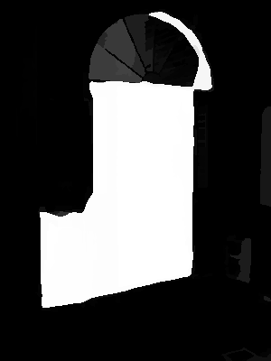
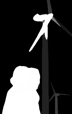
(a)	(b)	(c)	(d)

Figure 9: ISESS improving the saliency of wrogfully salient object partially highlighted by Auto-MSFNet. (a) original image; (b) label; (c) saliency map by Auto-MSFNet; (d) (c) enhanced by the proposed ISESS.

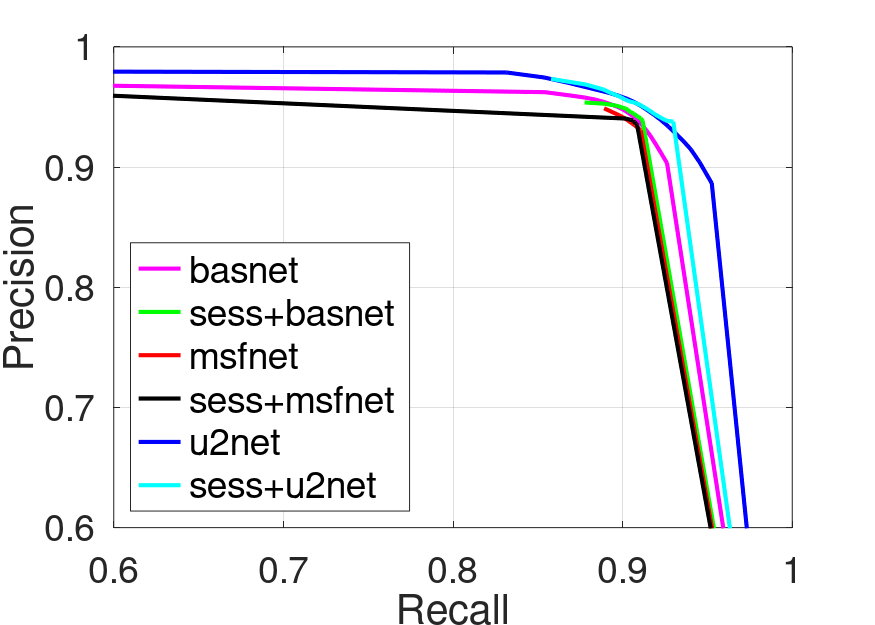
(a)	(b)	(c)

(d)	(f)

Figure 10: The Precision-Recall curves of all methods with and without enhancement in all datasets. (a) DUT_OMRON; (b) ECSSD; (c) HKU-IS; (d) ICOSEG; (e) SED2.

Sed2	$S_{m}$ $\uparrow$	$maxF_{\beta}$ $\uparrow$	$F_{\beta}^{w}$ $\uparrow$	$MAE$ $\downarrow$	$E_{\psi}^{m}$ $\uparrow$
U²Net	0.8193	0.8140	0.7704	0.0558	0.8529
U²Net+ISESS	0.8527	0.8404	0.8087	0.0483	0.8816
BASNET	0.8558	0.8565	0.8119	0.0514	0.8881
BASNET+ISESS	0.8643	0.8647	0.8375	0.0470	0.9037
Auto-MSFNet	0.8374	0.8333	0.8032	0.0544	0.8800
Auto-MSFNet+ISESS	0.8378	0.8518	0.8182	0.0524	0.8881
ECSSD	$S_{m}$ $\uparrow$	$maxF_{\beta}$ $\uparrow$	$F_{\beta}^{w}$ $\uparrow$	$MAE$ $\downarrow$	$E_{\psi}^{m}$ $\uparrow$
U²Net	0.9209	0.9286	0.8993	0.0370	0.9407
U²Net+ISESS	0.9182	0.9297	0.9099	0.0339	0.9467
BASNET	0.9142	0.9262	0.8992	0.0384	0.9414
BASNET+ISESS	0.9123	0.9267	0.9075	0.0355	0.9468
Auto-MSFNet	0.9067	0.9229	0.9032	0.0387	0.9427
Auto-MSFNet+ISESS	0.9069	0.9203	0.9026	0.0389	0.9411
DUT_OMRON	$S_{m}$ $\uparrow$	$maxF_{\beta}$ $\uparrow$	$F_{\beta}^{w}$ $\uparrow$	$MAE$ $\downarrow$	$E_{\psi}^{m}$ $\uparrow$
U²Net	0.8444	0.7868	0.7491	0.0541	0.8627
U²Net+ISESS	0.8418	0.7895	0.7647	0.0518	0.8736
BASNET	0.8362	0.7750	0.7465	0.0558	0.8607
BASNET+ISESS	0.8335	0.7758	0.7556	0.0548	0.8686
Auto-MSFNet	0.8321	0.7748	0.7536	0.049	0.8692
Auto-MSFNet+ISESS	0.8323	0.7730	0.7533	0.0491	0.8680
ICoSeg	$S_{m}$ $\uparrow$	$maxF_{\beta}$ $\uparrow$	$F_{\beta}^{w}$ $\uparrow$	$MAE$ $\downarrow$	$E_{\psi}^{m}$ $\uparrow$
U²Net	0.8727	0.8585	0.8210	0.0449	0.8957
U²Net+ISESS	0.8869	0.8769	0.8548	0.0404	0.9165
BASNET	0.8702	0.8578	0.8217	0.0476	0.8972
BASNET+ISESS	0.8784	0.8630	0.8397	0.0436	0.9057
Auto-MSFNet	0.8662	0.8515	0.8256	0.0425	0.9083
Auto-MSFNet+ISESS	0.8703	0.8544	0.8332	0.0417	0.9095
HKU-IS	$S_{m}$ $\uparrow$	$maxF_{\beta}$ $\uparrow$	$F_{\beta}^{w}$ $\uparrow$	$MAE$ $\downarrow$	$E_{\psi}^{m}$ $\uparrow$
U²Net	0.9183	0.9291	0.8950	0.0311	0.9453
U²Net+ISESS	0.9174	0.9292	0.9085	0.0274	0.9528
BASNET	0.9123	0.9264	0.8977	0.0308	0.9476
BASNET+ISESS	0.9110	0.9262	0.9075	0.0278	0.9536
Auto-MSFNet	0.9148	0.9297	0.9144	0.0255	0.9617
Auto-MSFNet+ISESS	0.9156	0.9270	0.9146	0.0255	0.9603

Table 1: Quantitative comparison between enhanced and non-enhanced maps in terms of $S_{m}$ $\uparrow$, $maxF_{\beta}$ $\uparrow$, $F_{\beta}^{w}$ $\uparrow$, $MAE$ $\downarrow$, and $E_{\psi}^{m}$ $\uparrow$. BLUE indicates the best result between the enhaced and non-enhanced maps.

4.4 Qualitative comparisons with non-enhanced maps

To visually evaluate the benefits of enhancing a saliency map using ISESS, we compiled images where ISESS improved different aspects of object representation (Figure 11). In the first two rows, there are images with minimal salient values in a small part of the desired objects (columns (c) and (g), on the first and second row, respectively). Even though the initial map provides little trust (i.e., small saliency values), ISESS created similar resulting maps using all deep models.

In the third and fourth rows, we present examples where ISESS captured most intended objects by extending the saliency value to regions with high similarity to the provided saliency. Note, however, that ISESS was unable to improve (e), even though (e) is a high precision map. Because the map is almost binary and most salient regions are taken as background queries, ISESS could not highlight the other salient regions.

The bottom four rows present images where ISESS was able to complete partially salient objects. Excluding the last row, each row shows simpler objects that the deep models failed to capture fully. In particular, in (e) and (g), ISESS could properly include a narrow stem coming out of the traffic light, even though narrow structures can be complex during superpixel delineation. The last image presents a successful case on a difficult challenge due to the radiating shadow coming out of the hole (which makes it hard to delineate adequate borders), especially on (e) where the initial map gave no part of the desired object.

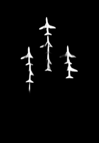
(a)	(b)	(c)	(d)	(e)	(f)	(g)	(h)

Figure 11: Mural of images with their initial saliency maps and their ISESS enhanced version. (a) original image; (b) ground-truth; (c) BASNET (Qin et al., 2019); (d) BASNET+ISESS; (e) Auto-MSFNet (Zhang et al., 2021); (f) Auto-MSFNet+ISESS; (g) U²Net (Qin et al., 2020); (h) U²Net + ISESS

5 Conclusion

We presented a hybrid model for saliency enhancement that exploits a loop between superpixel segmentation and saliency enhancement for the first time. ISESS delineates superpixels based on object information, as represented by an input saliency map, and improves the input saliency map by computing feature similarity between superpixels and queries. It exploits multiple scales of superpixel representation and integrates the intermediate saliency maps by cellular automata. Experimental results on five public SOD datasets demonstrate that ISESS can consistently improve object representation, especially in the following cases: (a) partially salient objects and (b) images with multiple salient objects with only a few captured by the deep model. Although better superpixel descriptors can be used for superpixel similarity, we focused on a simple color descriptor to illustrate how well deep models can be assisted by image-intrinsic information to improve their results.

We intend to explore ISESS enhanced maps for interactive- and co-segmentation tasks. The goal will be to assist humans when annotating images with fewer interactions, using the highly-trusted human-provided object location to define the precise background and foreground queries, combined with robust deep models to capture finer features. Another characteristic inherent in ISESS is the superpixel improvement over time. Although this aspect was not in focus in this paper, future work includes further evaluation of the enhancement loop’s impact on superpixel segmentation and how the final superpixel map can assist interactive object segmentation.

References

- Achanta et al. (2009) Achanta, R., Hemami, S., Estrada, F., Susstrunk, S., 2009. Frequency-tuned salient region detection, in: 2009 IEEE conference on computer vision and pattern recognition, IEEE. pp. 1597–1604.
- Al-Azawi (2021) Al-Azawi, M.A., 2021. Saliency-based image retrieval as a refinement to content-based image retrieval. ELCVIA: Electronic Letters on Computer Vision and Image Analysis 20, 0001–15.
- ”Belém et al. (2019) ”Belém, F., Guimarães, S.J., F., Falcão, A.X., 2019. Superpixel segmentation by object-based iterative spanning forest, in: Progress in Pattern Recognition, Image Analysis, Computer Vision, and Applications, Springer International Publishing. pp. 334–341.
- Belém et al. (2019) Belém, F., Melo, L., Guimarães, S., Falcão, A., 2019. The importance of object-based seed sampling for superpixel segmentation, in: Proc. 32nd Conf. Graphics Pattern Images (SIBGRAPI), pp. 108–115. To appear.
- Chen et al. (2018) Chen, B.C., Tao, X., Yang, M.R., Yu, C., Pan, W.M., Leung, V.C., 2018. A saliency map fusion method based on weighted ds evidence theory. IEEE Access 6, 27346–27355.
- Chen et al. (2014) Chen, L.C., Papandreou, G., Kokkinos, I., Murphy, K., Yuille, A.L., 2014. Semantic image segmentation with deep convolutional nets and fully connected crfs. arXiv preprint arXiv:1412.7062 .
- Chen et al. (2017) Chen, L.C., Papandreou, G., Kokkinos, I., Murphy, K., Yuille, A.L., 2017. Deeplab: Semantic image segmentation with deep convolutional nets, atrous convolution, and fully connected crfs. IEEE transactions on pattern analysis and machine intelligence 40, 834–848.
- Cheng et al. (2014) Cheng, M.M., Mitra, N.J., Huang, X., Torr, P.H., Hu, S.M., 2014. Global contrast based salient region detection. IEEE Transactions on Pattern Analysis and Machine Intelligence 37, 569–582.
- De Boer et al. (2005) De Boer, P.T., Kroese, D.P., Mannor, S., Rubinstein, R.Y., 2005. A tutorial on the cross-entropy method. Annals of operations research 134, 19–67.
- Falcão et al. (2004) Falcão, A.X., Stolfi, J., Lotufo, R.A., 2004. The image foresting transform: Theory, algorithms, and applications. IEEE Trans. Pattern Anal. Mach. Intell. 26, 19–29.
- He et al. (2016) He, K., Zhang, X., Ren, S., Sun, J., 2016. Deep residual learning for image recognition, in: Proceedings of the IEEE conference on computer vision and pattern recognition, pp. 770–778.
- He et al. (2015) He, S., Lau, R.W., Liu, W., Huang, Z., Yang, Q., 2015. Supercnn: A superpixelwise convolutional neural network for salient object detection. International journal of computer vision 115, 330–344.
- Huang et al. (2017) Huang, G., Liu, Z., Van Der Maaten, L., Weinberger, K.Q., 2017. Densely connected convolutional networks, in: Proceedings of the IEEE conference on computer vision and pattern recognition, pp. 4700–4708.
- Iqbal et al. (2020) Iqbal, E., Niaz, A., Memon, A.A., Asim, U., Choi, K.N., 2020. Saliency-driven active contour model for image segmentation. IEEE Access 8, 208978–208991.
- Jiang et al. (2013) Jiang, P., Ling, H., Yu, J., Peng, J., 2013. Salient region detection by ufo: Uniqueness, focusness and objectness, in: Proceedings of the IEEE international conference on computer vision, pp. 1976–1983.
- Lang et al. (2011) Lang, C., Liu, G., Yu, J., Yan, S., 2011. Saliency detection by multitask sparsity pursuit. IEEE transactions on image processing 21, 1327–1338.
- Li et al. (2018a) Li, L., Chai, X., Zhao, S., Zheng, S., Su, S., 2018a. Saliency optimization and integration via iterative bootstrap learning. International Journal of Pattern Recognition and Artificial Intelligence 32, 1859016.
- Li et al. (2018b) Li, X., Yang, F., Cheng, H., Liu, W., Shen, D., 2018b. Contour knowledge transfer for salient object detection, in: Proceedings of the European Conference on Computer Vision (ECCV), pp. 355–370.
- Liu and Heynderickx (2012) Liu, H., Heynderickx, I., 2012. Towards an efficient model of visual saliency for objective image quality assessment, in: 2012 IEEE International Conference on Acoustics, Speech and Signal Processing (ICASSP), IEEE. pp. 1153–1156.
- Liu et al. (2019) Liu, J.J., Hou, Q., Cheng, M.M., Feng, J., Jiang, J., 2019. A simple pooling-based design for real-time salient object detection, in: Proceedings of the IEEE/CVF Conference on Computer Vision and Pattern Recognition, pp. 3917–3926.
- Liu and Han (2016) Liu, N., Han, J., 2016. Dhsnet: Deep hierarchical saliency network for salient object detection, in: Proceedings of the IEEE conference on computer vision and pattern recognition, pp. 678–686.
- Luo et al. (2017) Luo, Z., Mishra, A., Achkar, A., Eichel, J., Li, S., Jodoin, P.M., 2017. Non-local deep features for salient object detection, in: Proceedings of the IEEE Conference on computer vision and pattern recognition, pp. 6609–6617.
- Máttyus et al. (2017) Máttyus, G., Luo, W., Urtasun, R., 2017. Deeproadmapper: Extracting road topology from aerial images, in: Proceedings of the IEEE International Conference on Computer Vision, pp. 3438–3446.
- Peng et al. (2016) Peng, H., Li, B., Ling, H., Hu, W., Xiong, W., Maybank, S.J., 2016. Salient object detection via structured matrix decomposition. IEEE transactions on pattern analysis and machine intelligence 39, 818–832.
- Qin et al. (2020) Qin, X., Zhang, Z., Huang, C., Dehghan, M., Zaiane, O.R., Jagersand, M., 2020. U2-net: Going deeper with nested u-structure for salient object detection. Pattern Recognition 106, 107404.
- Qin et al. (2019) Qin, X., Zhang, Z., Huang, C., Gao, C., Dehghan, M., Jagersand, M., 2019. Basnet: Boundary-aware salient object detection, in: Proceedings of the IEEE/CVF Conference on Computer Vision and Pattern Recognition, pp. 7479–7489.
- Qin et al. (2015) Qin, Y., Lu, H., Xu, Y., Wang, H., 2015. Saliency detection via cellular automata, in: Proceedings of the IEEE Conference on Computer Vision and Pattern Recognition, pp. 110–119.
- Simonyan and Zisserman (2014) Simonyan, K., Zisserman, A., 2014. Very deep convolutional networks for large-scale image recognition. arXiv preprint arXiv:1409.1556 .
- Singh and Kumar (2020) Singh, V.K., Kumar, N., 2020. Saliency bagging: a novel framework for robust salient object detection. The Visual Computer 36, 1423–1441.
- Su et al. (2019) Su, J., Li, J., Zhang, Y., Xia, C., Tian, Y., 2019. Selectivity or invariance: Boundary-aware salient object detection, in: Proceedings of the IEEE/CVF International Conference on Computer Vision, pp. 3799–3808.
- Tang et al. (2018) Tang, Z., Peng, X., Geng, S., Wu, L., Zhang, S., Metaxas, D., 2018. Quantized densely connected u-nets for efficient landmark localization, in: Proceedings of the European Conference on Computer Vision (ECCV), pp. 339–354.
- Tong et al. (2015) Tong, N., Lu, H., Ruan, X., Yang, M.H., 2015. Salient object detection via bootstrap learning, in: Proceedings of the IEEE conference on computer vision and pattern recognition, pp. 1884–1892.
- Vargas-Muñoz et al. (2019) Vargas-Muñoz, J.E., Chowdhury, A.S., Alexandre, E.B., Galvão, F.L., Miranda, P.A.V., Falcão, A.X., 2019. An iterative spanning forest framework for superpixel segmentation. IEEE Transactions on Image Processing 28, 3477–3489.
- Wang et al. (2021a) Wang, J., de Melo Joao, L., Falcão, A.X., Kosinka, J., Telea, A.C., 2021a. Focus-and-context skeleton-based image simplification using saliency maps., in: VISIGRAPP (4: VISAPP), pp. 45–55.
- Wang et al. (2021b) Wang, W., Lai, Q., Fu, H., Shen, J., Ling, H., Yang, R., 2021b. Salient object detection in the deep learning era: An in-depth survey. IEEE Transactions on Pattern Analysis and Machine Intelligence .
- Wang et al. (2003) Wang, Z., Simoncelli, E.P., Bovik, A.C., 2003. Multiscale structural similarity for image quality assessment, in: The Thrity-Seventh Asilomar Conference on Signals, Systems & Computers, 2003, Ieee. pp. 1398–1402.
- Wu et al. (2018) Wu, X., Ma, X., Zhang, J., Jin, Z., 2018. Salient object detection via reliable boundary seeds and saliency refinement. IET Computer Vision 13, 302–311.
- Yang et al. (2013) Yang, C., Zhang, L., Lu, H., Ruan, X., Yang, M.H., 2013. Saliency detection via graph-based manifold ranking, in: Proceedings of the IEEE conference on computer vision and pattern recognition, pp. 3166–3173.
- Zhang et al. (2018a) Zhang, J., Fang, S., Ehinger, K.A., Wei, H., Yang, W., Zhang, K., Yang, J., 2018a. Hypergraph optimization for salient region detection based on foreground and background queries. IEEE Access 6, 26729–26741.
- Zhang et al. (2016) Zhang, J., Sclaroff, S., Lin, Z., Shen, X., Price, B., Mech, R., 2016. Unconstrained salient object detection via proposal subset optimization, in: Proceedings of the IEEE conference on computer vision and pattern recognition, pp. 5733–5742.
- Zhang et al. (2018b) Zhang, L., Dai, J., Lu, H., He, Y., Wang, G., 2018b. A bi-directional message passing model for salient object detection, in: Proceedings of the IEEE Conference on Computer Vision and Pattern Recognition, pp. 1741–1750.
- Zhang et al. (2021) Zhang, M., Liu, T., Piao, Y., Yao, S., Lu, H., 2021. Auto-msfnet: Search multi-scale fusion network for salient object detection, in: ACM Multimedia Conference 2021, p. 667–676.
- Zhang et al. (2017) Zhang, P., Wang, D., Lu, H., Wang, H., Ruan, X., 2017. Amulet: Aggregating multi-level convolutional features for salient object detection, in: Proceedings of the IEEE International Conference on Computer Vision, pp. 202–211.
- Zhang et al. (2018c) Zhang, X., Wang, T., Qi, J., Lu, H., Wang, G., 2018c. Progressive attention guided recurrent network for salient object detection, in: Proceedings of the IEEE Conference on Computer Vision and Pattern Recognition, pp. 714–722.
- Zhao et al. (2019) Zhao, J.X., Liu, J.J., Fan, D.P., Cao, Y., Yang, J., Cheng, M.M., 2019. Egnet: Edge guidance network for salient object detection, in: Proceedings of the IEEE/CVF International Conference on Computer Vision, pp. 8779–8788.
- Zhu et al. (2014) Zhu, W., Liang, S., Wei, Y., Sun, J., 2014. Saliency optimization from robust background detection, in: Proceedings of the IEEE conference on computer vision and pattern recognition, pp. 2814–2821.