Lagrangian Manifestation of Anomalies in Active Turbulence

Abstract

We show that Lagrangian measurements in active turbulence bear imprints of turbulent and anomalous streaky hydrodynamics leading to a self-selection of persistent trajectories—Lévy walks—over diffusive ones. This emergent dynamical heterogeneity results in a super-diffusive first passage distribution which could lead to biologically advantageous motility. We then go beyond single-particle statistics to show that for the pair-dispersion problem as well, active flows are at odds with inertial turbulence. Our study, we believe, will readily inform experiments in establishing the extent of universality of anomalous behaviour across a variety of active flows.

Introduction

Flowing active matter, such as dense suspensions of bacteria, has emerged as one of the most intriguing class of problems in complex, driven-dissipative systems which sits at the intersection of non-equilibrium statistical physics, biophysics, soft-matter and of course fluid dynamics Marchetti et al. (2013); Ramaswamy (2017); Doostmohammadi et al. (2018); Alert et al. (2022). What makes such low Reynolds number systems particularly fascinating is the emergence of rich and complex collective patterns at scales much larger than, but driven by, relatively simpler individual dynamics Toner et al. (2005); Marchetti et al. (2013); Yeomans (2014); Ramaswamy (2017) as well as its ubiquity across systems as diverse as bacterial colonies (Wensink et al., 2012; Dunkel et al., 2013), suspensions of microtubules and molecular motors (Wu et al., 2017; Sanchez et al., 2012; Sumino et al., 2012), or schools of fish (Katz et al., 2011) and bird flocks (Marchetti et al., 2013; Ramaswamy, 2010; Cavagna et al., 2010). In dense active systems, typically those involving microscopic entities, the interactions between individual agents lead to unorganized, often vortical, dynamics with self-similar distribution of energy across several length scales. This last aspect, namely the appearance of the flow field and the power-laws which emerge in measurements of the kinetic energy across Fourier modes (Giomi et al., 2012; Wensink et al., 2012; Alert et al., 2020, 2022), lead to such states being called active turbulence in analogy with similar traits of high Reynolds number inertial turbulence (Alert et al., 2022).

However, there are important distinctions between inertial and active turbulence. The most striking of these being that unlike high Reynolds number flows, experiments suggest non-universal signatures of Lévy walks and anomalous diffusion in measurements of mean-square-displacements (MSDs) in active suspensions (Wu and Libchaber, 2000; Kurtuldu et al., 2011; Morozov and Marenduzzo, 2014; Ariel et al., 2015). These observations were substantiated in a recent theoretical work (Mukherjee et al., 2021) which showed not only the robustness of the anomalous diffusion and its coincidence with the emergence of novel, streaky structures in the flow for optimal activity, but also why in earlier theoretical studies C.P. and Joy (2020) such a scaling regime remained masked.

The fact that trajectories of tracers in such systems show Lévy statistics is consistent with other examples from the natural world where active agents Lévy walk or fly (Shlesinger et al., 1987; Dhar et al., 2006; Bychuk and O’Shaughnessy, 1994; Krummel et al., 2016; Cole, 1995). Nevertheless, this throws up interesting questions regarding the nature of trajectories and hence, fundamental issues of Lagrangian turbulence in such dense bacterial suspensions. In particular, a consequence of this could well be that while for low activities, trajectories are nearly always meandering (hence diffusive), at higher activities, there is a balance between those which follow Lévy statistics and those which do not. In fact, even for a given tracer it is conceivable that depending on the flow it experiences, its trajectory could either be persistent or random.

We address some of these issues relevant to dense (and dry) bacterial suspensions, by taking a continuum, numerical approach to the problem. The generalized hydrodynamic model (see, also, Refs. (Wensink et al., 2012; Zanger et al., 2015) for a detailed description), which is essentially a modified version of the Navier-Stokes equation employing terms that lead to pattern formation (similar to Swift-Hohenberg theory (Swift and Hohenberg, 1977)) and flocking behaviour (Toner-Tu theory (Toner and Tu, 1995, 1998)), is used to simulate the evolution of the coarse-grained velocity field ${\bf u}$ of bacterial suspensions, and is given as:

$$\partial_{t}{\bf u}+\lambda{\bf u}\cdot{\nabla\bf u}=-{\bf\nabla}p-\Gamma_{0}\nabla^{2}{\bf u}-\Gamma_{2}\nabla^{4}{\bf u}-(\alpha+\beta|{\bf u}|^{2}){\bf u}$$ (1)

where ${\bf u}$ satisfies the incompressibility constraint $\nabla\cdot{\bf u}=0$. The parameter $\lambda>1(<1)$ corresponds to pusher (puller)-type bacteria while the higher order derivatives along with the non-linear self-advective term drive the formation of chaotic flow patterns when $\Gamma_{0},\Gamma_{2}>0$. A key difference is that the usual diffusion term of the Navier-Stokes equation appears with the opposite sign, and acts towards inducing a turbulence instability in the bacterial system, while the additional bi-Laplacian term aids dissipation. The last term is a Toner-Tu drive (Toner and Tu, 1995, 1998), which is effectively a quartic Landau-potential for the velocity, with the activity $\alpha$ taking both positive (friction) and negative (active injection) values, while $\beta$ is strictly positive for stability and causes most of the momentum dissipation. For driven active systems ($\alpha<0$), this term leads to global polar ordering with a velocity $v_{0}=\sqrt{|\alpha|/\beta}$.

In our simulations, we solve Eq. (1) by using a de-aliased, pseudo-spectral algorithm on square, periodic domains of lengths $L\in\{20,40,80\}$ which are discretized by using $N^{2}\in\{1024^{2},4096^{2}\}$ collocation points. The simulations are performed for $5\times 10^{5}$ iterations with time-steps $\delta t=0.001$ and, in some cases, $\delta t=0.0002$ for higher temporal resolution (note that a simulation time of $\sim 30$ is $\sim 1$ minute of real time (Wensink et al., 2012)). The other parameters of the model are taken to be consistent with earlier studies (James and Wilczek, 2018; C. P. and Joy, 2020; Mukherjee et al., 2021; James et al., 2021), and these were carefully chosen to reproduce the physically observed flow patterns and Eulerian statistics (Wensink et al., 2012). Here, $\Gamma_{0}=0.045$, which corresponds to $-53$ $\mu m^{2}/s$, $\Gamma_{2}=\Gamma_{0}^{3}$ and $\lambda=3.5$ (Wensink et al., 2012). The swarming speed of Bacillus subtilis, which is linked to the activity, can vary over a wide range of $25-100$ $\mu m/s$, depending on the oxygen concentration of the system and the boundary conditions (Jánosi et al., 1998; Wensink et al., 2012; Sokolov and Aranson, 2012; Ariel et al., 2015). These velocities in the experiment are associated with the typical velocities which arise in the hydrodynamic description: $v_{\Gamma}=\sqrt{|\Gamma_{0}|^{3}/\Gamma_{2}}$ or $v_{0}=\sqrt{|\alpha|/\beta}$. An empirical comparison between simulations and experiments (see Wensink et al. (2012), Supporting Information) suggested that $\alpha=-1$ and $\beta=0.5$ (simulation units) corresponded to $-0.5/s$ and $4\times 10^{-4}s/\mu m^{2}$ (physical experimental units), respectively. These physical units correspond to a velocity scale $\sim 35\mu m/s$, with the corresponding simulation velocity scale $v_{0}=\sqrt{|\alpha|/\beta}=\sqrt{2}$. However, as was shown in a recent theoretical study (Mukherjee et al., 2021), phenomena like anomalous diffusion and Lévy walks, that were recently observed in experiments (Ariel et al., 2015), only become robust at sufficiently high activity levels in simulations (around $\alpha=-6$). Therefore, while keeping $\beta=0.5$ fixed, we vary the activity over a wide range $-6\leq\alpha\leq-1$. We note that the highest value of $\alpha=-6$ yields $v_{0}\approx 2.4\sqrt{2}$ (simulation units) or $v_{0}\approx 72\mu m/s$ (choosing, for convenience, the average velocity in the range $25\mu m/s-35\mu m/s$ reported by Wensink et al. (2012) as reference), which is well within the physically viable range of bacterial velocities (Wensink et al., 2012; Sokolov and Aranson, 2012). We caution the reader that this mapping of parameters should be seen as a rough guide, since the calibration of coefficients between theory and experiments is largely empirical. Lastly, the flow is seeded with $10^{5}$ randomly distributed tracers which evolve as $d{\bf x}/dt={\bf u}({\bf x}(t))$, with ${\bf x}(t)$ being the tracer location at time $t$, after a spinup time of $2\times 10^{4}$ iterations (when the flow reaches a statistically steady state). We use a fourth-order Runge-Kutta scheme, along with a bilinear interpolation scheme to obtain the fluid velocity at the particle positions ${\bf u}({\bf x}(t))$, to evolve the tracers with statistics being stored every $100$ iterations.

In Fig. 1(a) we show representative trajectories from our simulations with increasing levels of activity. While for suspensions with low activity ($\alpha=-1$), the particle motion is predominantly diffusive with large, knotted regions of random-walk, the more active fields ($\alpha=-4$) give rise to trajectories which have a persistent motion showing characteristic signatures of Lévy walks; a precise definition of the activity parameter $\alpha$ is given below. However, these Lévy-like, persistent trajectories are only one part of the story. Careful measurements in these simulations indicate that even at higher activity ($\alpha=-6$) it is easy to find in an ensemble trajectories that are persistent (Fig. 1(b)) and those that remain predominantly diffusive (Fig. 1(c)); see also https://youtu.be/CPJ3ZlXBf-k. (We note that the trajectories were artificially moved to a common center for visualization; in simulations, their origins are distributed randomly at different points in the flow.)

Figure 1: Representative trajectories for (a) suspensions with different degrees of activity $\alpha$ (see Eq. (1)) as well as for highly active suspensions showing the (b) fastest 1% tracers, that are persistent and anisotropic and (c) slowest 1% tracers that are diffusive and isotropic. Different trajectories are translated to a common origin for clarity and the color variation is a function of the angle at which they reach the bounding circle while the brightness is proportional to the density of trajectories; see also https://youtu.be/CPJ3ZlXBf-k. (These images, and Fig. 3, were generated with Processing (Reas and Fry, 2007; Pearson, 2011)).

This leads us to critically examine the nature of trajectories in such highly active systems and establish connections between anomalies of the emergent coarse-grained velocity field and its effect on the resultant Lagrangian statistics. As a result we uncover a remarkable dynamical heterogeneity in trajectories, implicit in Fig. 1, and its critical role in assisting the swarm for efficient foraging through first-passage statistics. We also show, in a way which is easily amenable to experiments, that such persistent motion are facilitated by the novel, emergent structures in the bacterial field—streaks—which have no known counterparts in inertial, high Reynolds number turbulence. We conclude by going beyond single-particle statistics and investigating the pair-dispersion problem in active turbulence.

Trajectories, especially for high activity, often comprise of long walking-segments of varying step-lengths, interspersed with turning points as seen in Figs. 1(a) and 1(b). Identifying the “turns” (Ariel et al., 2015; Mukherjee et al., 2021) is then crucial to segment trajectories into their constituent step-lengths (and waiting-times) for the analysis that follows. This is done by first calculating a turning angle $\theta$ at each point along the trajectory at time intervals $\Delta t$ as $\cos\left(\theta(t)\right)=\frac{\Delta\mathbf{r}(t)\cdot\Delta\mathbf{r}(t+\Delta t)}{|\Delta\mathbf{r}(t)||\Delta\mathbf{r}(t+\Delta t)|},$ where $\Delta\mathbf{r}(t)=\mathbf{r}(t)-\mathbf{r}(t-\Delta t)$; our results are insensitive for a wide range of $\Delta t$. Walking-segments and turns can be identified using a threshold $\theta(t)>\theta_{c}$, which in turn gives the step-lengths $d$ and waiting-times $\tau$ of the segments between successive turns. We choose $\theta_{c}=30^{\circ}$ for this study (Mukherjee et al., 2021) and have checked that our results remain unchanged for $25^{\circ}\leq\theta_{c}\leq 45^{\circ}$.

Fast and Slow Trajectories and The Role of Emergent Flow Structures

Do tracers in highly active suspensions ($\alpha=-6$) show a bias in the way they sample the relatively weaker and stronger vorticity $\omega=\nabla\times{\bf u}$ regions of the flow (Fig. 2(a))? The probability distribution function (pdf) of the vorticity field normalised by $\omega^{\prime}=\sqrt{\left\langle\omega^{2}\right\rangle}$, where $\left\langle\cdot\right\rangle$ denotes spatial averaging, along the Lagrangian trajectories and conditioned on the step-lengths $d$ shows (Fig. 2(f)) that trajectories are less likely to have persistent, directed motion in regions of strong vorticity: Quiescent regions favour persistent motion (Fig. 1(b)).

While this is a useful starting point, it does not capture the two main geometrical effects—vortical and straining regions—which characterise (inertial and active) two-dimensional turbulence. A first approach to this problem is through the Okubo-Weiss parameter $\Lambda=(\omega^{2}-\sigma^{2})/4\langle\omega^{2}\rangle$, where $\sigma^{2}=S_{ij}S_{ij}$ is the square of the strain-rate $S_{ij}=(\nabla\mathbf{u}+\nabla\mathbf{u}^{T})/2$, measured along individual trajectories: The sign of the Okubo-Weiss criterion (Okubo, 1970; Weiss, 1991) determines if the particle is either in a vortical ($\Lambda>0$) or a straining ($\Lambda<0$) region as shown in Fig. 2(b) for the Eulerian vorticity field of panel (a).

Figure 2(g)—the Lagrangian pdf of $\Lambda$, measured along particle tracks and conditioned on step-lengths in a manner similar to panel (f)—while clearly showing an overall preferential bias for vortical regions, brings out the inference drawn before more clearly. Tracers are far more likely to move in long, straight segments when they are in regions of the flow where both $\omega$ and $\Lambda$ have a small magnitude. This bias for persistent motion in quiescent regions of the flow is further affirmed by the joint distributions of tracer displacements $d$ with $\omega$ and $\Lambda$ as shown in Figs. 2(h) and 2(i), respectively. The insets in these panels are the same joint distributions but for $|\omega|$ and $|\Lambda|$. These clearly show that large displacements are more probable when both $\omega$ and $\Lambda$ are small: Long straight excursions instead of diffusive meandering occur in these regions.

These distributions, however, cannot trace the origins of extremely coherent motion of tracers, illustrated in Fig. 1(b), which contribute most to the anomalous diffusive behaviour in highly active suspensions. This is because a simple decomposition of the flow field in terms of vortical and straining regions fails to capture a recently discovered Mukherjee et al. (2021) additional emergent geometrical feature (with no counterpart in inertial turbulence): Streaks which are striped structures with alternate signs of $\omega$ as seen in Fig. 2(a).

Figure 2: Pseudocolor plots of the (a) vorticity $\omega$, (b) Okubo-Weiss parameter $\Lambda$ and (c) masked vorticity $\widetilde{\omega}$ fields showing the vortical, straining and streaky patches. Joint-distributions of the residence time and normalised distances of particles (d) within and (e) outside the streaks showing streaks facilitating enhanced displacement in shorter times. Probability distribution functions of the Lagrangian history of (f) vorticity and (g) Okubo-Weiss criterion, conditionally sampled over trajectory segment lengths $d$, show that persistent segments pass preferentially through quiescent regions of $\omega$ and $\Lambda$. Joint distributions of the segment lengths $d$ with (h) $\omega$ and (i) $\Lambda$ (insets show the distribution with $|\omega|$ and $|\Lambda|$) further emphasise that the longer trajectory segments mostly occur in quiescent field regions (the colorbar for the joint distributions shows logarithmically spaced decades).

Are streaks the primary cause for persistent Lévy walks seen in our Lagrangian measurements? In fact, the local flow geometry, and how it evolves in time, essentially governs the fate of a trajectory that passes through it. We demonstrate this in Fig. 3, which shows representative close-by trajectories originating in (a) vortical, (b) streaky or (c) quiescent straining regions; the color panels above the trajectories show the vorticity in the small region of the flow where these trajectories originate. This immediately brings out the striking difference in the fate of tracers depending on where they are in the flow. While particles originating in vortical spots (Fig. 3(a)) travel diffusively and incoherently, the ones which start in streaky regions (Fig. 3(b)) form a coherent bundle with persistent and correlated motions. Trajectories originating in quiescent regions (Fig. 3(c)) show elements of both diffusive motion with periods of persistence.

How, then, do we understand this puzzling behaviour? As the underlying field evolves, the trajectories which may have originated in a particular geometry of the flow are likely to encounter a different flow topology in time. This rules out mean-squared-displacements, conditioned on where trajectories originate, as a diagnostic for a couple of reasons. Firstly, such an exercise can be only performed up to short times during which the field remains largely unchanged. Secondly, these short-time time MSDs are invariably ballistic, regardless of where they originate. Hence, the subtle correlation between the emergent vagaries of the Eulerian field and the individual trajectories must be found within the Lagrangian history of particle dynamics.

But first, a sharper definition of what is a streak must be made which goes beyond the visual. To that end, careful measurements suggest that streaks coincide with places with (a) relatively moderate values of $\omega$ and (b) low magnitudes of $\Lambda$. This becomes clear upon comparing the vorticity field, in Fig. 2(a), with the $\Lambda$ field at the same time instance, shown in Fig. 2(b). This hints at a criterion, albeit somewhat ad-hoc, for identifying the streak regions. We define streaks as regions of the flow where, locally, the vorticity is bounded from below and the Okubo-Weiss criterion is bounded from above, i.e., $\omega\geq\omega_{T}$ and $\Lambda\leq\Lambda_{T}$; we choose (and other similar choices give equally consistent results) thresholds $\omega_{T}=0.5\omega^{\prime}$ and $\Lambda_{T}=0.1\Lambda^{\prime}$. This criterion allows us to define a mask which, when applied to the vorticity field of active flows, generates a filtered field $\widetilde{\omega}=\omega$ in streaks and 0 otherwise. In Fig. 2(c) we show $\widetilde{\omega}$ for the same flow realisation as in panel (a) to demonstrate the accuracy of this criterion which goes beyond the binary classification of the Okubo-Weiss parameter and picks out the streaky regions.

With the definitions of the flow topologies in place, we can now unambiguously separate trajectories based on the flow regions they encounter. An obvious quantification is the joint distribution of tracer displacements $s$ with residence times $t$ in and out of streak regions. Since the streaky regions occupy a relatively small area-fraction $A_{f}$ of the flow, it is useful to look at the effective displacements $\phi\equiv s/\sqrt{A_{f}}$ within a streak, and conversely $\phi\equiv s/(1-\sqrt{A_{f}})$ outside it, to ascertain the relative degree to which streaky and non-streaky regions assist persistent motion.

While streaks form a small fraction ($\sim 12\%$) of the flow resulting in a relatively smaller residence time, tracers inside the (Fig. 2(d)) streaks are advected much farther within this short time than those outside (Fig. 2(e)). The joint $\phi-t$ distribution is much wider when outside these special structures, indicating that large residence times (in purely vortical and straining patches) do not lead to large displacements. Thus, coherent, persistent motion is intrinsically correlated with the special flow patterns (Fig. 2(c)) that a bacterial suspension can spontaneously generate.

First Passage Problem and Dynamical Heterogeneity

This surprising ability to exploit self-generated patterns and their emergent hydrodynamics to aid persistent motion accords individuals a distinct advantage to reach targets—for nutrition, for example—on much shorter time scales than it would be otherwise possible. While this was certainly implicit in earlier observations of anomalous diffusion through measurements of the mean-square-displacements Mukherjee et al. (2021), a direct way of looking at this is to ask how such activity-induced streaks enhance the efficacy of tracers in reaching distances $R$ away. This, of course, is the much studied question in statistical physics of First Passage Problems (Chandrasekhar, 1943; Bray et al., 2013; Redner, 2001; Balakrishnan, 2021; Metzler et al., 2014), also used to quantify biological motility (Chou and D’Orsogna, 2014; Bisht et al., 2017; Teimouri and Kolomeisky, 2019): What is the statistics of the time $t_{R}$ for tracers to reach (for the first time and be “absorbed” at) the boundary of a circle of radius $R$ as illustrated in Fig. 1; see also https://youtu.be/CPJ3ZlXBf-k.

Figure 3: Representative bundles of trajectories originating in (a) vortical spots, (b) streaks and (c) quiescent regions. While the trajectories spread incoherently in (a) and coherently in (b), there is a mix of both for (c). The trajectories are coloured, varying smoothly from blue (left edge) to black (right edge), based upon their $x$-coordinates with the colour and gives a sense of mixing vis-à-vis coherence in the trajectory bundles.

In the context of bacterial suspensions and living systems in general, the first passage characteristics are critical to how efficiently bacteria forage for food and survive. In an active turbulent flow, whose evolution is governed by Eq. (1), a bacterium foraging for food can be thought of as a point tracer being advected until it reaches the food source at a distance $R$, at which point the search is concluded.

The probability of a tracer reaching (and being absorbed by) a boundary $R$ at time $t=t_{R}$ when it starts from $r=0$ at $t=0$ is given by the first passage probability distribution $P(R,t_{R})$ which is calculated from the (survival) probability $S(t)=\int_{0}^{R}p(r,t)2\pi rdr$ of not reaching the boundary in time $t_{R}$ via $P(R,t_{R})=-\frac{\partial S}{\partial t}\big{|}_{t_{R}}$ (Balakrishnan, 2021; Siegert, 1951). The survival probability assumes isotropy of the distribution $p(r,t)$ of tracers which, for low activities, satisfies the diffusion equation (Risken and Frank, 1996) with absorbing boundary condition $p(R,t)=0$ and the initial condition $p(r,0)=\delta(r)/2\pi r$. We begin by writing the Fokker-Planck equation in two-dimensions:

$$\partial_{t}p(r,t)=K_{d}\nabla^{2}p(r,t)$$ (2)

$K_{d}$ being the diffusion constant. Assuming a solution of the form $p(r,t)=u(r)f(t)$ yields separate differential equations for the temporal and radial parts to obtain:

$$u(r) =J_{0}(Cr)=\sum^{\infty}_{n=0}\frac{(-1)^{n}}{(n!)^{2}}\left(\frac{Cr}{2}\right)^{2n}$$ (3)

$$f(t) =f_{0}e^{-C^{2}K_{d}t}$$ (4)

where $f_{0}=f(t)|_{t=0}$, and $J_{0}$ is the Bessel function of the first kind and order zero. By using the absorbing boundary condition to solve for the radial part $u(r)$, the delta-function initial condition to determine $f_{0}$ and the constraint that $S(t=0)=1$, we obtain

$$p(r,t)=\frac{1}{2\pi R^{2}\left(\sum_{i}\frac{J_{1}(h_{i})}{h_{i}}\right)}\sum_{i}J_{0}\left(\frac{h_{i}r}{R}\right)e^{-h_{i}K_{d}t/R^{2}};$$ (5)

thence the survival probability

$$S(t)=\int_{0}^{R}p(r,t)2\pi rdr=\sum_{i}e^{-h_{i}K_{d}t/R^{2}}\frac{J_{1}(h_{i})}{h_{i}}.$$ (6)

Here, $J_{1}$ is the Bessel function of the first kind and order one, whereas $h_{i}$ are the zeros of $J_{0}(CR)$. The first passage time distribution is then simply

$$P(R,t_{R})=-\partial_{t}S|_{t=t_{R}}=\frac{K_{d}}{R^{2}}\sum_{i}e^{-h_{i}K_{d}t_{R}/R^{2}}J_{1}(h_{i})$$ (7)

The dominant contribution to the first passage distribution comes from the smallest $h_{i}=A$ and yields the well-known result: $P(R,t_{R})\sim\frac{K_{d}}{R^{2}}e^{-AK_{d}t_{R}/R^{2}}$  (Verma et al., 2020). The first passage distribution can be generalised to the case of anomalous diffusion as $P(R,t_{R})\sim e^{-t_{R}/R^{2/\xi}}$, where the scaling exponent $1\leq\xi\leq 2$ is a consequence of the anomalous diffusion in the mean-square-displacement $\Delta x^{2}\sim t^{\xi}$ (and which can also be obtained analytically by solving the fractional Fokker-Planck equation (Siegert, 1951; Rangarajan and Ding, 2000a, b; Gitterman, 2000; Palyulin et al., 2019)).

In the inset of Fig. 4(a) we show the first passage time distributions for different values of $R$ which collapse on to a unique curve when the first passage times are scaled as $t_{R}/R^{2}$ (Fig. 4(a)) consistent with our theoretical prediction for moderately active suspensions. On making suspensions more active, as shown in Fig. 4(b), the diffusive $t_{R}/R^{2}$ scaling still remains approximately true but only for large values of $R$. Indeed, for smaller values of $R$ (Fig. 4(b), inset), the distributions collapse only when the first passage times are scaled as $t_{R}/R^{3/2}$, accounting for the enhanced motility. This is because at such short distances, persistent trajectories contribute to the statistics of first passage overwhelmingly and hence the scaling exponent associated with anomalous diffusion in such systems, $\xi\approx 4/3$ Mukherjee et al. (2021), leads to an anomalous form of the first passage distribution.

While the normalized first passage distributions give a statistical sense for an ensemble of trajectories, it does not allow us to have a sense of the variations, within an ensemble, of individual trajectories. Since tracers sample the entire phase space, the issue of an incipient dynamical heterogeneity in the flow is a vexing one.

In order to understand this, we take a fraction ($10\%$, for sufficient statistics) of the fastest and slowest trajectories that reach various target radii $R$, for different values of $\alpha$. Visually, the fastest and slowest trajectories are different: The former mostly straight and persistent, while the latter convoluted and meandering for all levels of activity. However, the Lagrangian history of these tracers, i.e., the $\Lambda$ values they encounter before hitting their targets, shows, as illustrated in the inset of Fig. 4(c) that at mild levels of activity there is no distinction between the underlying Eulerian field sampled by the fastest and slowest tracers. These conditional distributions of the Okubo-Weiss parameter show that the heterogeneity in trajectories, up to intermediate levels of activity, is simply a statistical consequence of the random sampling of the flow. However, for highly active suspension, where anomalous diffusion becomes robust, signatures of dynamical heterogeneity, as seen in the clearly different Lagrangian histories of the fastest and slowest trajectories (see Fig. 4(c), manifest themselves. Consistent with the findings so far that persistent motion favours quiescent field regions, the fastest tracers sample milder regions of the Okubo-Weiss field, in comparison to the slowest tracers. This distinction, moreover, is starker for smaller $R$ values, while at large values of $R$, the tracers begin to experience (statistically) similar underlying fields.

This evidence for dynamical heterogeneity in the flow, such that the variation in the nature of trajectories is not merely statistical as happens in inertial turbulence (Scatamacchia et al., 2012), is further strengthened by looking at where in the flow do the fastest and slowest tracers originate, for a given value of $R$. In other words, do trajectories get lucky by being at the right place at the right time, which allows them to reach their targets faster than others? This would suggest that for highly active suspensions, the initial locations of these fast, lucky trajectories must be clustered in nearby regions while for less active flows they are more uniformly distributed. In the inset of Fig. 4(d), we show a plot of the starting points of the fastest $1\%$ of the trajectories for a target at $R=15$. We indeed find that for the highly active suspensions ($\alpha=-6$) these points remain strongly clustered, unlike the random and uniform distribution seen for the less active ($\alpha=-1$) case. While confirming a dynamically heterogeneous flow, this also explains the bundling of these trajectories already seen in Fig. 1(b), where the fastest tracers (after their initial locations are artificially superimposed at the center of the circle), evolve as coherent bundles, arriving at their target circle and forming a very anisotropic distribution around the circumference. This is because the bundles originate clustered together in a few special locations in the flow and hence follow very similar trajectories. We quantify the degree of this clustering by calculating the pair-distribution function $g(r)$, for the fastest and slowest $1\%$ of the tracers, in Fig. 4(d). The $g(r)$ of the origins of the slowest tracers quickly attains a value close to $1$, irrespective of activity, corresponding to a uniform (or ideal-gas) distribution of points (albeit with a small overshoot for $\alpha=-6$ at small $r$, showing weak preferential clustering also for the slowest tracers). The fastest tracer origins for high activity show a pronounced peak in the pair distribution at small values of $r$, reflecting the presence of these lucky spots. At mild activity, the $g(r)$ for the fastest tracer origins rapidly attains to a value of $1$ as well, reflecting the fact that the heterogeneity of trajectories is merely statistical.

Figure 4: (a) Semi-log plots of the first passage distributions for mildly active suspensions collapse on a single curve for rescaled time $t_{R}/R^{2}$ corresponding the diffusive transport for different values of $R$; the inset shows the same without the rescaling of time. (b) Analogous plots for highly active suspensions show a similar diffusion-driven collapse only for large distances and time; for short distance (inset) the curves collapse when time is rescaled as $t_{R}/R^{3/2}$ which factors in anomalous diffusion. (c) Probability distribution functions of $\Lambda$ conditioned on the fastest (solid-lines) and slowest (dashed-lines) $10\%$ of tracers for $\alpha=-6$ and $\alpha=-4$ (inset) and for various target radii $R$. The distributions differ only for the highly active suspension and for small $R$ showing the emergence of a true dynamical heterogeneity. This is visually illustrated in the inset of panel (d) showing that the origins of the fastest $1\%$ tracers for $\alpha=-1$ are randomly distributed whereas those for $\alpha=-6$ are strongly localised suggesting “lucky” spots for efficient motility. This is confirmed in (d) measurements of the pair-distribution function which gives a pronounced peak for the fastest tracer origins for $\alpha=-6$, while rapidly converging to the uniform distribution $g(r)=1$. Similar measurements for the fastest tracers for lower activity and indeed for the slowest trajectories for all activity show uniform distribution throughout.

Pair-Dispersion

So far we have focussed our attention on single-particle statistics. But before we conclude, we must consider the implications of these anomalies on the Richardson-Obukhov pair-dispersion problem (Richardson and Walker, 1926; Obukhov, 1941) which informs much of our understanding of inertial turbulence (Salazar and Collins, 2009). Pair-dispersion is simply the statistics of separation of particle pairs that originate within a small distance $\epsilon$ of each other measured as $\left\langle r_{p}^{2}(t)\right\rangle=\left\langle|{\mathbf{x}_{1}(t)}-{\mathbf{x}_{2}(t)}|^{2}\right\rangle$, where $\mathbf{x}_{1}(t)$ and $\mathbf{x}_{2}(t)$ are the positions of a particle pair, with $|\mathbf{x}_{1}(0)-\mathbf{x}_{2}(0)|=\epsilon$ being their initial separation, and $\left\langle{\cdot}\right\rangle$ denotes averaging over all particle pairs.

Figure 5(a) shows pair-separation for increasingly active suspensions, with $\epsilon=0.001$. Interestingly, the influence of activity appears to be mild, with only a slight change in the extent of the intermediate scaling; even for $\alpha=-6$, a scaling regime seems to extend only up to a decade. The limited extent of scaling, and its significant deviation from the Richardson prediction $\sim t^{3}$ for inertial turbulence, may stem from the lack of an inertial range in active turbulence. It has been shown that active turbulence, at least using the nematohydrodynamic model and other minimal models for wet active nematics (Urzay et al., 2017; Carenza et al., 2020; Alert et al., 2022), does not have an energy cascade resulting from non-linear mode interactions. While, admittedly, our model differs from these, it is likely that a similar situation arises here. In fact, the presence of a particularly wide inertial range and scale separation (effectively, a large Reynolds number) is essential to observe the Richardson scaling regime even in inertial turbulence, despite cascade dynamics, and persistent motion in trajectories (ballistic Lévy walks) can further lead to deviation from Richardson scaling (Boffetta and Sokolov, 2002). While there is no natural way to increase scale separation in our system, we tested various domain sizes for $\alpha=-6$, from $L=20$ (on $N=1024$) to $L=80$ (on $N=4096$), and obtained identical pair-separation curves, without an increase in the extent of scaling. The inset of Fig.5(a) shows the influence of the initial separation $\epsilon$ on pair-separation for $\alpha=-6$. As $\epsilon$ decreases, the slope of the intermediate range increases significantly. This $\epsilon$ dependence is consistent with findings from two-dimensional inertial turbulence (Rivera and Ecke, 2005; Xia et al., 2019), and the apparent steepening of the slope is a consequence of an exponential initial separation tending to diffusive separation at longer times.

In the absence of robust Richardson scaling, other pair-separation measures have been proposed to quantify dispersion statistics (Jullien et al., 1999; Boffetta and Sokolov, 2002). One such is the probability distribution of pair-separations $r_{p}$, at different times during the growth of $\left\langle r_{p}^{2}\right\rangle$. Figure 5(b) shows the probability distribution of the rescaled (with the variance) pair-separations $s_{p}=r_{p}/\sigma$, at various time instances, for trajectories with an initial separation of $\epsilon=0.001$ and for $\alpha=-6$. The separations $s_{p}$ collapse to a single stretched-exponential distribution while at very long times, well into the diffusive pair-separation regime $\left\langle r_{p}^{2}\right\rangle\sim t$, the $s_{p}$ distribution becomes Gaussian. All this is consistent with findings from two-dimensional inertial turbulence (Jullien et al., 1999; Rivera and Ecke, 2005), where a stretched-exponential and Gaussian distribution of rescaled separations is found for the forward enstrophy-cascade and inverse energy-cascade regimes, respectively. This shows that the pair-separation process is self-similar in time, following different distributions during the rapid and (eventually) diffusive growth.

Related to the first passage problem, we consider the distribution of separation doubling-times (Boffetta and Sokolov, 2002; Rivera and Ecke, 2005). This is defined as the time $t_{d}$ it takes for an initial separation $r_{p}$ to grow to a scale $\rho r_{p}$. Here, we can also expect an influence of the persistence in trajectories. Smaller initial separations $r_{p}$ will lead to longer correlated motion, as trajectory-pairs will sample similar flow geometries (Fig. 3). This would lead to relatively longer doubling times, and a wider $t_{d}$ distribution. At large initial separations, where trajectory-pairs are essentially uncorrelated to begin with, the separation doubling will occur more rapidly. This is precisely what is observed in Fig. 5(c) for $\rho=1.8$; our results are similar for other $\rho$ values that are not too small. The distributions of doubling-times $t_{d}$, normalized by the mean doubling time $\left\langle{t_{d}}\right\rangle$, for small values of $r_{p}$, follow a stretched exponential function, similar to two-dimensional inertial turbulence in the enstrophy-cascade range (Rivera and Ecke, 2005). The distributions become steeper with increasing $r_{p}$, reflecting the decorrelation within trajectory pairs. The inset of Fig. 5(c) shows that at very large values of $r_{p}$, deep into the diffusive pair-separation phase, the distribution of $t_{d}$, as anticipated, approaches a Gaussian.

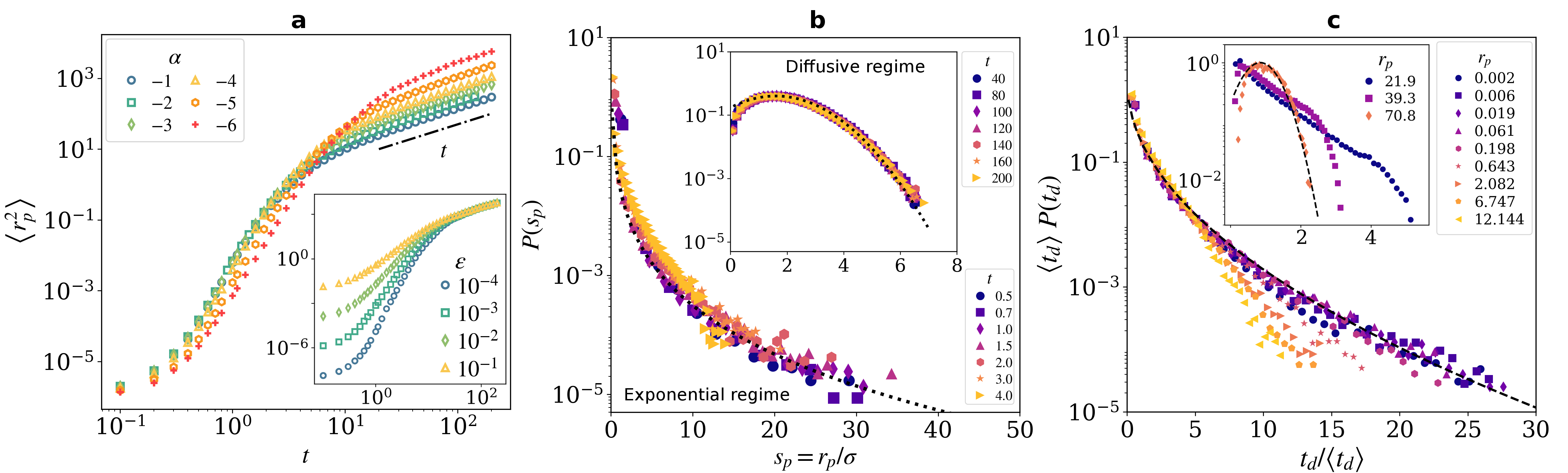
Figure 5: (a) The dependence of the relative pair separation on $\alpha$ (with $\epsilon=0.001$) and (inset) on $\epsilon$ (for $\alpha=-6$). (b) Probability distribution of the normalized pair separation $s_{p}$ follows a stretched exponential for times up to diffusive pair-separation, whence (inset) the distribution becomes Gaussian. (c) The probability distribution of pair-separation doubling times $t_{d}$ are also stretched exponentials at small separations; the curves become steeper with increasing $r_{p}$ and (inset) converge to a Gaussian distribution for large $r_{p}$.

Conclusions

Anomalous diffusion and Lévy walks are common place in a wide variety of biological systems. However, in dense suspensions of microorganisms, such as bacterial swarms, which are a typical example of flowing active matter and a testing ground for active turbulence, the experimental evidence for such phenomena is only recent (Ariel et al., 2015). Furthermore, theoretical studies have been unable to go beyond the simple diffusion picture and predict, detect or understand the emergence of such super-diffusive regimes in active turbulence. This issue was resolved by a recent work (Mukherjee et al., 2021) showing that anomalous Lagrangian statistics manifest only in extremely active suspensions, with $\alpha\sim-6$. Further exploring such highly active suspensions consistently revealed signatures of anomalies in Lagrangian measurements. The streaky flow regions, together with an emergent dynamical heterogeneity, contrive to selectively propel tracers persistently and aid in anomalous first-passage statistics. The results presented in this work should be readily amenable to experimental measurements in super-diffusive bacterial swarms, as well as in a diverse class of active flows. Whether the conjoined emergence of Eulerian streaks at high activity, and their role in promoting persistent motion, is universal, remains to be ascertained, and the true mechanisms for manifesting Lagrangian anomalies may well be system dependent. Notwithstanding, we feel that our results show a biologically crucial aspect of the generalized hydrodynamics model beyond what has been previously observed, extending its applicability to a realm closer to experimental observations.

Further, measures like pair-dispersion mirror fundamental quantities like Lyapunov exponents, that characterize chaos in both diverging trajectories and solutions of the hydrodynamic equations. For instance, the flow Lyapunov exponent is known to increase with Reynolds number in inertial turbulence approximately as $\sim\mathrm{Re}^{1/2}$ (Mukherjee et al., 2016; Boffetta and Musacchio, 2017; Berera and Ho, 2018). The analogous effect of activity on Lyapunov exponents in active turbulence remains unknown and is part of ongoing work, both within the Eulerian (Mukherjee et al., 2016; Boffetta and Musacchio, 2017; Berera and Ho, 2018) and Lagrangian framework Bec et al. (2006); Ray (2018), which looks at different aspects of many-body chaos (Murugan et al., 2021) in such systems. Indeed, a complete understanding of the dynamical facets of active turbulence calls for a complete characterization of the skeleton of chaos underlying active flows. It is interesting to note that a recent work (Kiran et al., 2022) on the (Lagrangian) irreversibility in such suspensions shows similar anomalies between active and inertial turbulence. Lastly, our work also lays out a systematic framework for the Lagrangian analysis of active flows, including measures for identifying geometrical structures emerging in the Eulerian fields. Adopting these in future work will not only ascertain the extent of universality of active turbulence anomalies, but also help connect hydrodynamic theories of active matter more closely to the physical picture.