Blow-up lemma for cycles in sparse random graphs

Abstract

In a recent work, Allen, Böttcher, Hàn, Kohayakawa, and Person provided a first general analogue of the blow-up lemma applicable to sparse (pseudo)random graphs thus generalising the classic tool of Komlós, Sárközy, and Szemerédi. Roughly speaking, they showed that with high probability in the random graph $G_{n,p}$ for $p\geq C(\log n/n)^{1/\Delta}$, sparse regular pairs behave similarly as complete bipartite graphs with respect to embedding a spanning graph $H$ with $\Delta(H)\leq\Delta$. However, this is typically only optimal when $\Delta\in\{2,3\}$ and $H$ either contains a triangle ($\Delta=2$) or many copies of $K_{4}$ ($\Delta=3$). We go beyond this barrier for the first time and present a sparse blow-up lemma for cycles $C_{2k-1},C_{2k}$, for all $k\geq 2$, and densities $p\geq Cn^{-(k-1)/k}$, which is in a way best possible. As an application of our blow-up lemma we fully resolve a question of Nenadov and Škorić regarding resilience of cycle factors in sparse random graphs.

1 Introduction

Problems concerning embedding a spanning graph $H$ into a host graph $G$ under various conditions have always been among the most challenging topics to study in extremal combinatorics. One of the strongest tools in this area is certainly the blow-up lemma of Komlós, Sárközy, and Szemerédi [27]. It led to several deep and beautiful results, some gems including spanning trees [26, 30], powers of Hamilton cycles [28], $H$-factors [29], bounded degree subgraphs [9], and many more. We refer an interested reader to great surveys and gentle introduction into using the blow-up lemma and related tools [31, 34, 48].

In order to apply it the host graph $G$ is required to be highly structured and dense, in a sense that it contains $\Omega(n^{2})$ edges, which is perhaps its main drawback. A natural next step is to ask whether this powerful tool can be ‘transferred’ to a sparse setting, in which the host graph has only $o(n^{2})$ edges. Arguably the most interesting and thoroughly studied instances of such graphs are (pseudo)random graphs, notably the binomial Erdős-Rényi random graph $G_{n,p}$. (see [10] for an overview of some influential research regarding transference of combinatorial results to a sparse random setting).

In context of a sparse blow-up lemma, the host graph $G$ would ideally be given as a collection of sparse regular pairs. For $p\in[0,1]$ and $\varepsilon>0$ a pair of sets $(V_{1},V_{2})$ is $(\varepsilon,p)$-regular (in a graph $G$) if for every $V_{i}^{\prime}\subseteq V_{i}$, $i\in\{1,2\}$, with $|V_{i}^{\prime}|\geq\varepsilon|V_{i}|$, the density $d(V_{1}^{\prime},V_{2}^{\prime})$ of edges between $V_{1}^{\prime}$ and $V_{2}^{\prime}$ in $G$ is such that

$$|d(V_{1},V_{2})-d(V_{1}^{\prime},V_{2}^{\prime})|\leq\varepsilon p.$$

However, this basic notion of regularity is not sufficient for embedding a spanning graph $H$ even for $p=1$, as $(\varepsilon,1)$-regular pairs can have isolated vertices. An $(\varepsilon,p)$-regular pair $(V_{1},V_{2})$ is said to be $(\varepsilon,\alpha,p)$-super-regular if additionally every $v\in V_{i}$ satisfies $\deg_{G}(v,V_{3-i})\geq(1-\varepsilon)|V_{3-i}|\alpha p$, for $i\in\{1,2\}$. Then the original blow-up lemma [27] says $H$ can be embedded into a certain collection of $(\varepsilon,\alpha,p)$-super-regular pairs. Rather unfortunately, it is known that this cannot be adapted in a straightforward way to a setting in which $p$ is an arbitrary decreasing function of the number of vertices of $H$—for instance, there are graphs on vertex set $V_{1}\cup V_{2}\cup V_{3}$ where each $(V_{i},V_{j})$ is $(\varepsilon,1,p)$-super-regular, but contain no triangles (see [18, 24]). Hence, further strengthening is needed.

One such strengthening was proposed by Balogh, Lee, and Samotij [5] in a work on triangle factors in subgraphs of random graphs. In a graph $G$, sets $\{V_{i}\}_{i\geq 2}$ which are pairwise $(\varepsilon,\alpha,p)$-super-regular are said to have the regularity inheritance property if for every $V_{i},V_{j},V_{k}$ and $v\in V_{i}$, the pair $\big{(}N_{G}(v,V_{j}),N_{G}(v,V_{k})\big{)}$ is $(\varepsilon,p)$-regular of density at least $d(V_{j},V_{k})-\varepsilon p$, inheriting regularity from the pair $(V_{j},V_{k})$. Using this definition they proved that with high probability for $p\gg(\log n/n)^{1/2}$ every subgraph $G$ of $G_{n,p}$ on sets $\{V_{i}\}_{i\in[3]}$ of linear size which are pairwise $(\varepsilon,\alpha,p)$-super-regular and have the regularity inheritance property, contains a disjoint collection of triangles covering all of its vertices. This result can be considered as the first real blow-up type statement for sparse graphs.

Allen, Böttcher, Hàn, Kohayakawa, and Person [2] recently established several sought-after variants of a general blow-up lemma for sparse random and pseudorandom graphs together with many relevant applications. Simply put, they showed that for every $\Delta\geq 2$, w.h.p. in the random graph $\Gamma\sim G_{n,p}$, if $p\gg(\log n/n)^{1/\Delta}$, any $r$-colourable graph $H$ on $n$ vertices with $\Delta(H)\leq\Delta$ and colour classes $X_{1}\cup\dotsb\cup X_{r}$, can be found as a subgraph of every graph $G\subseteq\Gamma$ on vertex set $\{V_{i}\}_{i\in[r]}$, with $|V_{i}|=|X_{i}|$, where every $(V_{i},V_{j})$ is $(\varepsilon,\alpha,p)$-super-regular and $\{V_{i}\}_{i\in[r]}$ have the regularity inheritance property. This on one hand completes the quest for a ‘general version’ of the blow-up lemma applicable to sparse graphs, putting many results concerning embedding large graphs into the random graph $G_{n,p}$ under a unified framework, but on the other leaves a major question unresolved: how sparse can the graph $G$ actually be?

The assumption $p\gg(\log n/n)^{1/\Delta}$ poses a both ‘natural’ and ‘technical’ barrier. The former is reflected in the fact that at this point the random graph allows for a ‘vertex-by-vertex’ type of embedding schemes as typically every set of at most $\Delta$ vertices has a large common neighbourhood. The latter, and arguably more difficult to surpass, is related to the regularity inheritance property. It is known (see [17]) that in an $(\varepsilon,p)$-regular pair most sets of size $\Omega(1/p)$ inherit regularity. Consequently, regularity inheritance can only be established if the density $p$ is such that $|N_{G}(v,V_{i})|\gg 1/p$, and as typically $|N_{\Gamma}(v,V_{i})|\approx np$, this forces $p\gg n^{-1/2}$. That being said, the sparse blow-up lemma of [2] is optimal up to the log factor when $\Delta=2$ and $H$ contains a triangle, but also when $\Delta=3$ and $H$ contains many copies of $K_{4}$ (for more precise details see [2, Section 7.2]). However, this lower bound on $p$ is probably very far from the truth in the general case.

The main result of this paper is to break this barrier and show a variant of the sparse blow-up lemma which is applicable at much lower densities. In order to fully and precisely state our result we need a definition. A pair $(V_{1},V_{2})$ is said to be $(\varepsilon,p)$-lower-regular if for every $V_{i}^{\prime}\subseteq V_{i}$, with $|V_{i}^{\prime}|\geq\varepsilon|V_{i}|$, the density $d(V_{1}^{\prime},V_{2}^{\prime})$ satisfies $d(V_{1}^{\prime},V_{2}^{\prime})\geq d(V_{1},V_{2})-\varepsilon p$. Let $\mathcal{G}_{\mathrm{exp}}^{k}(C_{t},n,\varepsilon,p)$ denote the class of graphs whose vertex set is a disjoint union $V_{1}\cup\dotsb\cup V_{t}$, with all $V_{i}$ of size $n$, $(V_{i},V_{i\pm 1})$ forms an $(\varepsilon,p)$-regular pair of density $(1\pm\varepsilon)p$, and every $v\in V_{i}$ satisfies: $\deg_{G}(v,V_{i\pm 1})=(1\pm\varepsilon)np$, $|N_{G}^{j}(v,V_{i\pm j})|\geq(1-\varepsilon)(np)^{j}$ for every $j\in[k-1]$, and

• if $t=2k-1$, $(N_{G}^{k-1}(v,V_{i+(k-1)}),N_{G}^{k-1}(v,V_{i-(k-1)}))$ is $(\varepsilon,p)$-lower-regular;

• if $t=2k$, $(N_{G}^{k-1}(v,V_{i+(k-1)}),V_{i+k})$ and $(N_{G}^{k-1}(v,V_{i-(k-1)}),V_{i-k})$ are $(\varepsilon,p)$-lower-regular.

Theorem 1.1.

Let $k\geq 2$ and $t\in\{2k-1,2k\}$. For every $\alpha>0$, there exists a positive $\varepsilon$ with the following property. For every $\mu>0$, there is a $C>0$ such that if $p\geq Cn^{-(k-1)/k}$, then w.h.p. $\Gamma\sim G_{n,p}$ satisfies the following. Every $G\subseteq\Gamma$ which belongs to $\mathcal{G}_{\mathrm{exp}}^{k}(C_{t},\tilde{n},\varepsilon,\alpha p)$, with $\tilde{n}\geq\mu n$, contains a disjoint collection of cycles $C_{t}$ covering all vertices of $G$.

This is the first variant of the blow-up lemma, that the author is aware of, in which the density $p$ is significantly smaller than $n^{-1/2}$ (or $n^{-1/\Delta}$ for that matter), making all the extremely convenient things that come along regularity inheritance void. Importantly, we do not require $G$ to exhibit the regularity inheritance property among all pairs/triples of sets in $\{V_{i}\}_{i\geq 2}$ but only expansion along the edges of $C_{t}$ as stated above. This is a rather reasonable assumption, as w.h.p. the underlying random graph $G_{n,p}$ behaves in a similar way.

The value $p\geq Cn^{-(k-1)/k}$ is optimal in the following way. Suppose $p=o(n^{-(k-1)/k})$. Then w.h.p. in $\Gamma\sim G_{n,p}$ every set of size $\varepsilon(np)^{k-1}$ expands to at most $2\varepsilon(np)^{k}=o(n)$ vertices, so no $G\in\mathcal{G}_{\mathrm{exp}}^{k}(C_{2k},\tilde{n},\varepsilon,\alpha p)$ appears as a subgraph of $\Gamma$. It may well be that imposing a different natural condition on top of regularity is not sufficient to go below this bound. Perhaps the only room for improvement regarding density would be requiring that every vertex of $G$ belongs to $\Omega(n^{t-1}p^{t})$ copies of $C_{t}$, or in other words, a positive fraction of all copies it closes in $G_{n,p}$. Optimistically, under this assumption one can hope to go all the way down to the natural bound $p\geq Cn^{-(t-2)/(t-1)}$, at which point w.h.p. all copies of $C_{t}$ can be removed from $G_{n,p}$ by deleting a tiny proportion of all edges and the regularity setting stops making sense.

Our proof is based on the absorbing method, which is discussed in great detail in Section 2. The theorem itself is then proven in Section 4. Akin to both [5] and [2], we showcase the usefulness of our blow-up lemma by providing an optimal resilience result for the random graph $G_{n,p}$ with respect to containing a $C_{t}$-factor.

Resilience of (random) graphs has received a lot of attention lately, ever since the paper of Sudakov and Vu [52] who first coined down the term officially (even though implicitly it had been studied before, see e.g. [3]).

Definition 1.2.

Let $G$ be a graph and $\mathcal{P}$ a monotone graph property. We say that $G$ is $\alpha$-resilient with respect to $\mathcal{P}$, for some $\alpha\in[0,1]$, if $G-H$ contains $\mathcal{P}$ for every $H\subseteq G$ with $\deg_{H}(v)\leq\alpha\deg_{G}(v)$ for all $v\in V(G)$.

This notion is in the literature known as local resilience. Many of the famous results in extremal combinatorics can be looked at through the lenses of resilience. A prime example of those is Dirac’s theorem [12]: every graph on $n$ vertices with minimum degree $\delta(G)\geq n/2$ contains a Hamilton cycle. In other words, the complete graph on $n$ vertices $K_{n}$ is $(1/2)$-resilient with respect to Hamiltonicity. Problems of this type have recently been intensively studied in sparse random graphs by several groups of researchers. Some of the most notable results include Hamiltonicity [36, 38, 44], almost spanning trees [4], triangle factors [5], powers of Hamilton cycles [16, 50], bounded degree spanning subgraphs [2, 8]; for more see the excellent surveys [7, 51] and references therein.

Huang, Lee, and Sudakov [21] were the first to study resilience of dense random graphs, that is when $p$ is a fixed constant, with respect to having an (almost-)$H$-factor, for general $H$. Later, as a consequence of resolving the counting version of the infamous KŁR-conjecture, Conlon, Gowers, Samotij, and Schacht [11] extended this for $p=o(1)$. In both a leftover is present, namely the obtained collection of copies of $H$ covers all but a small fraction of vertices—hence an almost-$H$-factor. Most recently, Nenadov and Škorić [45] went even further and precisely determined conditions under which the random graph $G_{n,p}$ is w.h.p. resilient with respect to (almost-)$H$-factors and the leftover one cannot avoid. Among other things they posed a conjecture regarding $C_{t}$-factors and highlighted it as one of the more challenging problems to resolve. As the main application of our blow-up lemma we confirm their conjecture.

Theorem 1.3.

Let $k\geq 2$ and $t\in\{2k,2k+1\}$. For every $\alpha>0$, there exists a positive $C$ such that if $p\geq Cn^{-(k-1)/k}$, then w.h.p. $\Gamma\sim G_{n,p}$ is $(1/\chi(C_{t})-\alpha)$-resilient with respect to containing a $C_{t}$-factor.

This can be viewed as an extension of the result of Balogh, Lee, and Samotij [5] from triangles to longer cycles, and is an improvement of the result of Allen, Böttcher, Ehrenmüller, and Taraz [1] for all cycles of length at least four. (In the latter, the result for $C_{4}$ and $C_{5}$ is already optimal up to the $(\log n)^{1/2}$ factor in the density $p$, which we now get rid of.)

Our result is optimal in almost every aspect. Firstly, resilience value can be seen to be the best possible for $C_{2k}$ by choosing a set of size $n/2-1$ (for even $n$) and disconnecting it from the rest of the graph. As for $C_{2k+1}$, it seems like the correct value should depend on the so-called critical chromatic number $\chi_{\mathrm{cr}}(H)$, defined as

$$\chi_{\mathrm{cr}}(H)=\frac{(\chi(H)-1)v(H)}{v(H)-\sigma(H)},$$

where $\sigma(H)$ is the size of the smallest colour size in a colouring of $H$ with $\chi(H)$ colours (for more details on why this should be the correct parameter, we refer the reader to [25, 35]). In particular, the resilience value for $C_{2k+1}$ in that case would be $k/(2k+1)$ which is significantly larger than $1/3$ for every $k\geq 2$. We believe that the importance of obtaining such a result only for odd cycles does not outweigh the technical difficulties one would face and do not pursue this direction further.

Secondly, the density $p$ is asymptotically optimal. In order to see this, assume $t=5$ and let $v$ be an arbitrary vertex of $\Gamma$. Consider the second neighbourhood of $v$, $N_{\Gamma}^{2}(v)$, and remove all of the edges with both endpoints lying in it. Obviously, this prevents $v$ from being in a copy of $C_{5}$ and moreover, the number of edges removed from any $u\in N_{\Gamma}^{2}(v)$ is roughly $(np)^{2}p$ (this requires proof, see [45]) which is much smaller than $np$ if $p\ll n^{-1/2}$. This principle can be extended to ‘isolate’ more than just one vertex $v$ and works similarly for every $t\geq 3$; for more details and precise results for general $H$ we refer the reader to [45].

The proof of Theorem 1.3 involves a standard argument using the sparse regularity method and the blow-up lemma (Theorem 1.1) and is presented in Section 5. There are some intricacies to it, but this is nothing much out of the ordinary. We see it vaguely plausible that some of our methods, specifically from the proof of the blow-up lemma, may be applied in order to obtain a more general result regarding $H$-factors in random graphs under certain restrictions.

Notation.

We let $[n]:=\{1,\dotsc,n\}$. For $x,y,\varepsilon\in\operatorname*{\mathbb{R}}$ we write $x\in(y\pm\varepsilon)$ to denote $y-\varepsilon\leq x\leq y+\varepsilon$. We use standard asymptotic notation $o$, $O$, $\omega$, and $\Omega$, and use $f\ll g$ for $f=o(g)$ and $f\gg g$ for $f=\omega(g)$. Floors and ceilings are suppressed whenever they are not crucial. If we write e.g. $D_{3.3}$, this is to mean that the value $D$ is the one featured in the statement of Lemma/Proposition/Claim 3.3. Let $G=(V,E)$ be a graph. For a vertex $v\in V(G)$ and a set $X\subseteq V(G)$, we use $N_{G}^{i}(v,X)$ to denote the set of vertices $x\in X$ for which there is a $vx$-path of length $i$ (consisting of $i$ edges) in $G$; then $N_{G}(v,X)$ stands for $N_{G}^{1}(v,X)$. We use $N_{G}^{i}(v)$ to denote the $i$-th neighbourhood of $v$, that is $N_{G}^{i}(v):=N_{G}^{i}(v,V(G))$. Perhaps deviating from standard notation, we let $G-X$ be the graph obtained from $G$ by removing a set of vertices $X$, and $G-\nabla(X)$ the graph on the same vertex set as $G$ obtained by removing all edges with at least one endpoint in $X$ from $G$. The $2$-density of a graph $H$, denoted by $m_{2}(H)$, is defined as $m_{2}(H):=\max_{H^{\prime}\subseteq H}(e(H^{\prime})-1)/(v(H^{\prime})-2)$, where $H^{\prime}$ ranges over all subgraphs with at least two edges. For a graph $H$ on vertices $\{1,\dotsc,t\}$, $\mathcal{G}(H,n,\varepsilon,p)$ is the class of graphs $G$ whose vertex set is a disjoint union $V_{1}\cup\dotsb\cup V_{t}$, with all $V_{i}$ of size $n$, and $(V_{i},V_{j})$ forms an $(\varepsilon,p)$-regular pair of density $(1\pm\varepsilon)p$ if and only if $ij\in E(H)$, these being the only edges of $G$. A canonical copy of a graph $H$ in $G$ is a set $\{v_{1},\dotsc,v_{t}\}$ for which $v_{i}\in V_{i}$ for every $i\in[t]$ and $v_{i}v_{j}\in E(G)$ for every $ij\in E(H)$.

2 How to prove the blow-up lemma

Consider a subgraph $G\subseteq\Gamma$ of $\Gamma\sim G_{n,p}$ which also belongs to $\mathcal{G}_{\mathrm{exp}}^{k}(C_{t},\tilde{n},\varepsilon,\alpha p)\subseteq\mathcal{G}(C_{t},\tilde{n},\varepsilon,\alpha p)$. If aiming only to find a very large collection of $t$-cycles in $G$, one could just employ the resolution of the KŁR-conjecture in random graphs, due to Saxton and Thomason [49] and independently Balogh, Morris, and Samotij [6] (see [11] for a statement most similar to the one tailored to random graphs as below and [43] for a new simplified proof).

Theorem 2.1 (KŁR Conjecture).

For every graph $H$ and every $\alpha>0$, there exists a positive constant $\varepsilon$ with the following property. For every $\mu>0$, there is a positive constant $C$ such that if $p\geq Cn^{-1/m_{2}(H)}$, then w.h.p. $\Gamma\sim G_{n,p}$ satisfies the following. Every $G\subseteq\Gamma$ which belongs to $\mathcal{G}(H,\tilde{n},\varepsilon,\alpha p)$, with $\tilde{n}\geq\mu n$, contains a canonical copy of $H$.

The theorem above gives only one copy of a graph $H$, but combined with the ‘slicing lemma’ it easily gives $(1-o(1))\tilde{n}$ disjoint copies.

Lemma 2.2.

Let $0<\varepsilon_{1}<\varepsilon_{2}\leq 1/2$, $p\in(0,1)$, and let $(V_{1},V_{2})$ be an $(\varepsilon_{1},p)$-regular pair. Then for every $V_{i}^{\prime}\subseteq V_{i}$, $i\in[2]$, of size $|V_{i}^{\prime}|\geq\varepsilon_{2}|V_{i}|$, the pair $(V_{1}^{\prime},V_{2}^{\prime})$ is $(\varepsilon_{1}/\varepsilon_{2},p)$-regular of density $d(V_{1},V_{2})\pm\varepsilon_{1}p$.

On a very abstract level, the proof strategy for Theorem 1.1 is now very natural and simple: iteratively find copies of $C_{t}$ until there are only some $\varrho\tilde{n}$ vertices remaining uncovered in each $V_{i}$, and then do something to cover those as well. This ‘something’ is a brilliant technique very widely used in a variety of settings nowadays—the absorbing method.

The absorbing method has been a key ingredient of numerous results in extremal combinatorics regarding finding spanning structures both in dense and sparse regimes. At the heart of the method lies the following idea. One would like to find a certain (usually highly structured) graph $A\subseteq G$ and a designated set $W\subseteq V(A)$, which allow for a great deal of flexibility when constructing the desired spanning graph $\mathcal{S}$. Namely, no matter how we manage to embed a fixed subgraph $\mathcal{S}^{\prime}\subseteq\mathcal{S}$ into $G$ so that it covers all $V(G)\smallsetminus V(A)$ and potentially uses some vertices of $W$, the leftover vertices $V(G)\smallsetminus V(\mathcal{S}^{\prime})$ can be ‘absorbed’ into a complete embedding of $\mathcal{S}$. Usually we have no control over which vertices of the designated set $W$ are used in this partial embedding, so for this to work, the method fully depends on a very careful choice of the graph $A$—it must be capable of completing the embedding no matter which vertices of $W$ are already used. This technique first explicitly appeared in the work on Hamilton cycles in hypergraphs by Rödl, Ruciński, and Szemerédi [47], but was previously used implicitly in the works of Erdős, Gyárfas, and Pyber [13], and Krivelevich [32]. As of today, there is quite a substantial body of work in (random) graph theory utilising the absorbing method (for some specific examples, see e.g. [19, 23, 37, 39, 40, 41] and for a very non-standard application we have drawn some inspiration from, a recent result [15]).

2.1 Absorbers in sparse regular pairs

Our goal is to find a graph $A$ and a designated set $W$ in a subgraph $G$ of $G_{n,p}$ belonging to $\mathcal{G}_{\mathrm{exp}}^{k}(C_{t},\tilde{n},\varepsilon,\alpha p)$, which have the capability of ‘absorbing’ the leftover vertices remaining after applying Theorem 2.1 to $G-V(A)$. The first step in a usual way of doing this is to find many disjoint absorbers. An $R$-absorber, in our context, is a graph $F$ which is rooted at a set of vertices $R=\{r_{1},\dotsc,r_{t}\}$ and is such that both $F$ and $F-R$ have a $C_{t}$-factor. Then the graph $A$ is obtained by constructing disjoint absorbers rooted on some strictly prescribed $t$-element sets $R\subseteq W$.

Of course, if we were just aiming to construct many disjoint absorbers rooted at some sets $R\subseteq W$, we could turn to Theorem 2.1, as long as the absorber $F$ is of constant size. However, for the absorbing property to be established, it is absolutely necessary that the roots of the absorbers are chosen in a certain way which makes it impossible to employ this strategy—Theorem 2.1 has no power of embedding graphs for which some vertices are already fixed. A cheap attempt at repairing this would be to take one of the prescribed $t$-element sets $R=\{r_{1},\dotsc,r_{t}\}$ and apply it with their neighbourhoods $N_{G}(r_{1}),\dotsc,N_{G}(r_{t})$. Unfortunately, by looking at neighbourhoods the regularity between sets is lost, as typically a vertex $v\in V(G)$ has neighbourhood of size $np\ll n$ for $p=o(1)$ which is not sufficiently large to ‘inherit’ the $(\varepsilon,p)$-regularity. (Actually, sets of size $1/p$ typically inherit regularity as well, see [17], but this is still not enough when $p=o(n^{-1/2})$.)

A slightly less cheap attempt, and a natural extension of this, is to ‘expand’ the neighbourhoods of every $r_{1},\dotsc,r_{t}$ some $\ell\geq 1$ times until $|N_{G}^{\ell}(r_{i})|\geq\delta\tilde{n}$, for some $\delta>\varepsilon>0$, and then apply Theorem 2.1 with $N_{G}^{\ell}(r_{i})$. Based on the density $p\gg n^{-(k-1)/k}$, one expects this to happen when $(np)^{\ell}\gg n$, i.e. when $\ell=k$. As a dummy example of how this works consider the following scenario with $k=2$ and an absorber $F$ for $C_{4}$ from Figure 1(b). For every $r_{i}$ find a set $S_{i}\subseteq N_{G}^{2}(r_{i})$ of size at least $\delta\tilde{n}$ (as $(np)^{2}\gg n$ this is feasible), so that for every $s_{i}\in S_{i}$ there is a copy of the graph on Figure 1(a) between $r_{i}$ and $s_{i}$. These sets and graphs are chosen to be disjoint for different $i$. As $S_{i}$’s are sufficiently large and ‘inherit regularity’, we can apply Theorem 2.1 with them to find the $4$-cycle $s_{1},\dotsc,s_{4}$ with $s_{i}\in S_{i}$ which then, due to the special choice of sets $S_{i}$, completes a copy of $F$ in $G$. Of course, the real graph $F$ is going to be much more complex as well as the whole procedure. In order for this to work it is of utmost importance that an $R$-absorber $F$ is ‘locally sparse’, or in other words each $N_{F}^{j}(r_{i})$, $r_{i}\in R$, is an independent set for all $1\leq j\leq k-1$. Otherwise, for reasons going along the lines of what is said in previous paragraphs, we cannot ensure that an edge with both endpoints in some $N_{F}^{j}(r_{i})$ exists in $N_{G}^{j}(r_{i})$.

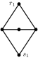
(a) Dummy $C_{4}$-switcher

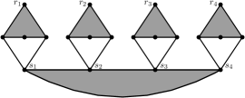
(b) Dummy $C_{4}$-absorber

Figure 1: A dummy example of an absorber (right) and its building block (left)

Lastly, let us mention that the graph $A$ cannot be built in $G$ by greedily stacking disjoint $R$-absorbers. Namely, there are $\varrho\tilde{n}$ vertices to ‘absorb’, and even in the best case with $R$-absorbers being of constant size, there are also roughly $\varrho\tilde{n}$ such graphs we need to ‘greedily stack’. As $G$ is living in $G_{n,p}$ and has minimum degree roughly $np\ll n$, already after $np$ iterations of using a greedy construction we potentially run out of space: it can easily happen that the whole neighbourhood of some vertex $w\in W$ which is prescribed to be the root is already taken. This is circumvented by using Haxell’s matching condition (see Theorem 3.5 below), and all the absorbers are to be found in one fell swoop.

2.2 Switchers, absorbers, and other graph definitions

Before defining an $R$-absorber we break its structure into even smaller pieces which we call switchers. A switcher with respect to a $C_{t}$-factor (whenever we say ‘switcher’ we mean ‘switcher with respect to a $C_{t}$-factor’), is a graph $H$ which contains specified vertices $u$ and $v$ and is such that both $H-v$ and $H-u$ have a $C_{t}$-factor. A construction that first comes to mind is to take a path on $t-1$ vertices and connect its endpoints to both $u$ and $v$ (see Figure 1(a)). However, such a graph contains $C_{4}$ as a subgraph, and as we plan on finding absorbers within sparse regular pairs, and $m_{2}(C_{4})=3/2$, we should not hope to find anything that has $C_{4}$ as a subgraph at density $p=o(n^{-2/3})$, or whenever $k\geq 4$ (equivalently, $t\geq 7$). It turns out that finding a suitable construction as above is easier said than done.

Let $T$ be a $(t-1)$-ary tree of depth $k$ rooted at a vertex $v$. Replace every vertex of $T$ by a $t$-cycle $C_{t}$ and choose an arbitrary vertex from the cycle on depth $0$ as the root and label it by $v$. Additionally, for every edge of $T$, identify any two vertices belonging to two cycles corresponding to endpoints of the edge in such a way that every vertex, other than $v$ and $(t-1)^{k+1}$ vertices belonging to the cycles on depth $k$, belong to exactly two cycles. We say that a graph obtained this way is a $C_{t}$-tree of depth $k$ rooted at $v$. We usually omit saying ‘of depth $k$’ and ‘rooted at $v$’ when this is clear from the context. The definition of a $C_{t}$-tree has a much more natural visual representation, as shown on Figure 2.

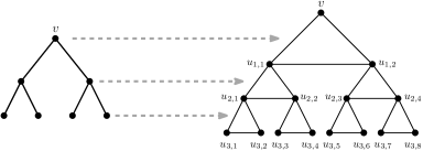
Figure 2: An example of a $C_{3}$-tree of depth $k=2$.

One may think of the vertices of a $C_{t}$-tree as arranged on levels with $v$ as the root, and level $i$ consisting of $(t-1)^{i}$ vertices split into groups of $t-1$, each group closing a cycle with one (distinct) vertex on level $i-1$ (see Figure 2 again).

For ease of reference, which is used later in the proof, we label the vertices of a $C_{t}$-tree:

• (level $0$): vertex $v$ is considered to be the root and gets label $u_{0,1}$;

• (levels $1$ to $k+1$): vertices belonging to a cycle together with a vertex $u_{i,j}$, for some $0\leq i\leq k$, $1\leq j\leq(t-1)^{i}$, get labels $u_{i+1,(j-1)(t-1)+1},u_{i+1,(j-1)(t-1)+2},\dotsc,u_{i+1,(j-1)(t-1)+t-1}$ such that

  $$u_{i,j},u_{i+1,(j-1)(t-1)+1},\dotsc,u_{i+1,(j-1)(t-1)+t-1}$$

  is a $t$-cycle in a $C_{t}$-tree.

We next list several graphs which are used as gadgets in order to construct switchers and combine them into an $R$-absorber.

An $(a,b)$-ladder of length $\ell$, for $\ell$ odd, is a graph $G$ defined as follows:

• the vertex set of $G$ is

  $$V(G)=\bigcup_{\begin{subarray}{c}i\in[\ell]\\ i\text{ odd}\end{subarray}}\{w_{i,1},\dotsc,w_{i,a}\}\cup\bigcup_{\begin{subarray}{c}i\in[\ell]\\ i\text{ even}\end{subarray}}\{w_{i,1},\dotsc,w_{i,b}\};$$

• $w_{1,1},\dotsc,w_{\ell,1}$ and $w_{1,a},w_{2,b},\dotsc,w_{\ell-1,b},w_{\ell,a}$ are paths of length $\ell-1$;

• $w_{i,1},\dotsc,w_{i,a}$ is a path for every odd $i$;

• $w_{i,1},\dotsc,w_{i,b}$ is a path for every even $i$.

So this graph looks like a ‘ladder’ where the ‘steps’ are paths of two different alternating lengths (see Figure 3).

Figure 3: An example of a $(2,3)$-ladder of length $\ell=7$.

Two $t$-cycles, $v_{1},\dotsc,v_{t}$ and $u_{1},\dotsc,u_{t}$, are said to be $k$-ladder-connected if there exist an $(a_{1},b_{1})$-ladder and an $(a_{2},b_{2})$-ladder, both of length $2k-1$, which are vertex-disjoint and such that:

• $a_{1}=k-1$, $a_{2}=t-k$, $b_{i}=t-a_{i}$, for $i\in\{1,2\}$;

• vertices $\{w_{1,j}\}_{j\in[a_{1}]}$ and $\{w_{1,j}\}_{j\in[a_{2}]}$ are identified with $v_{2},\dotsc,v_{k}$ and $v_{k+1},\dotsc,v_{t}$;

• vertices $\{w_{2k-1,j}\}_{j\in[a_{1}]}$ and $\{w_{2k-1,j}\}_{j\in[a_{2}]}$ are identified with $u_{2},\dotsc,u_{k}$ and $u_{k+1},\dotsc,u_{t}$;

Two $C_{t}$-trees of depth $k$ rooted at $v$ and $v^{\prime}$ are said to be $k$-ladder-connected if their respective cycles given by the vertices on the $k$-th and $(k+1)$-st levels are all pairwise $k$-ladder-connected. That is, for every $j\in[(t-1)^{k}]$, the two cycles

$$u_{k,j},u_{k+1,(j-1)(t-1)+1},\dotsc,u_{k+1,(j-1)(t-1)+t-1}\enskip\text{and}\enskip u_{k,j}^{\prime},u_{k+1,(j-1)(t-1)+1}^{\prime},\dotsc,u_{k+1,(j-1)(t-1)+t-1}^{\prime}$$

are $k$-ladder-connected. Finally, say that a graph obtained this way is a $(v,v^{\prime})$-switcher and denote it by $F_{\mathrm{sw}}$; indeed, it contains a $C_{t}$-factor in both $F_{\mathrm{sw}}-v$ an $F_{\mathrm{sw}}-v^{\prime}$, see Figure 4.

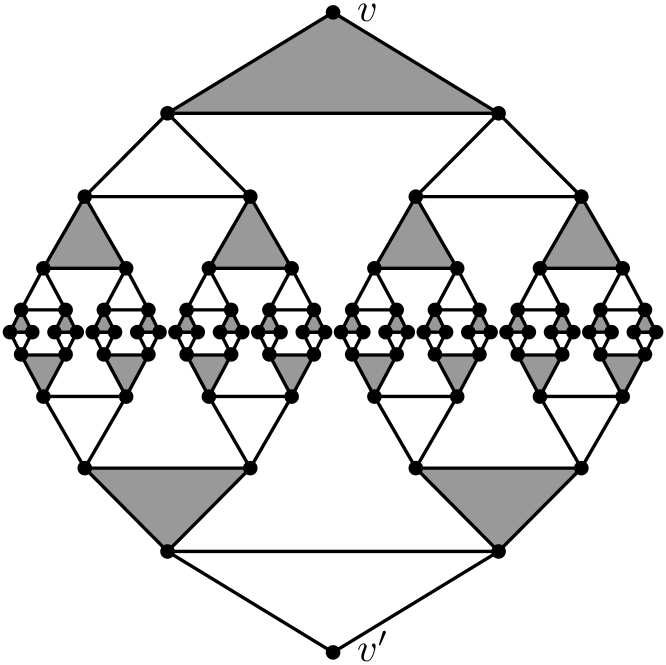
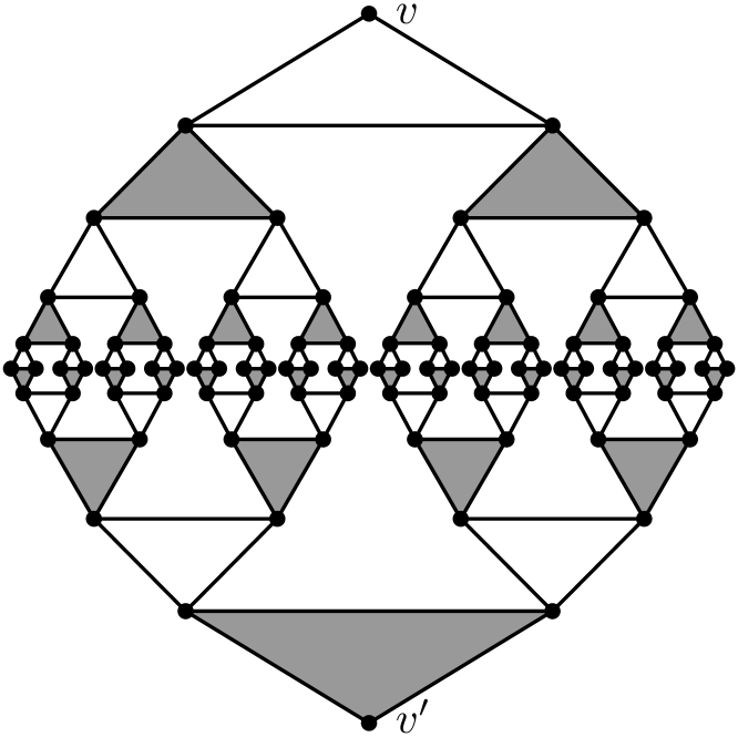
Figure 4: An example of a $(v,v^{\prime})$-switcher $F_{\mathrm{sw}}$ with two $C_{3}$-factors. The figure on the left represents a $C_{3}$-factor in $F_{\mathrm{sw}}-v$ and the figure on the right represents a $C_{3}$-factor in $F_{\mathrm{sw}}-v^{\prime}$.

An $R$-absorber $F_{\mathrm{abs}}$ for a set $R=\{r_{1},\dotsc,r_{t}\}$ is a graph which consists of a $t$-cycle $s_{1},\dotsc,s_{t}$ and a collection of disjoint $(s_{i},r_{i})$-switchers $F_{\mathrm{sw}}$ for every $i\in[t]$. We let $F_{\mathrm{conn}}$ denote the graph obtained by contracting every $C_{t}$-tree of depth $k-1$ (not $k$!) rooted at $r_{i}$ of $F_{\mathrm{abs}}$ individually into a vertex and $F_{\mathrm{abs}}^{-}$ the subgraph of $F_{\mathrm{abs}}$ obtained by removing those $C_{t}$-trees. The proof of the following proposition is rather straightforward (but tedious) and for cleaner exposition we postpone it to the appendix.

Proposition 2.3.

Let $k\geq 2$ and $t\in\{2k-1,2k\}$. Then the $R$-absorber $F_{\mathrm{abs}}$ satisfies the following:

1. both $F_{\mathrm{abs}}$ and $F_{\mathrm{abs}}-R$ have a $C_{t}$-factor,

2. $m_{2}(F_{\mathrm{conn}})\leq k/(k-1)$, and

3. $F_{\mathrm{abs}}$ is a subgraph of $\mathcal{G}(C_{t},v(F_{\mathrm{abs}}),0,1)$.

2.3 From $R$-absorbers to the highly structured graph $A$

Finally, in order to build the graph $A$ from $R$-absorbers, we rely on a so-called template graph. The first usage of this strategy goes back to Montgomery [39] and is highly versatile when one has to absorb several vertices at the same time. We make use of the following straightforward generalisation of [42, Lemma 6.1] which is itself a slight modification of [39, Lemma 10.7] of Montgomery. It turns out to be a bit more tailored to our needs as opposed to the original lemma.

Lemma 2.4.

There is an integer $m_{0}$ such that, for every $m\geq m_{0}$, there exists a $t$-partite $t$-uniform hypergraph $B$ on vertex classes $B_{1},\dotsc,B_{t}$, with $|B_{i}|=2m$ and $\Delta(B)\leq 40^{t}$, as well as sets $B_{i}^{\prime}\subseteq B_{i}$, with $|B_{i}^{\prime}|=m$, satisfying the following. For every $Z\subseteq\bigcup_{i\in[t]}B_{i}^{\prime}$ with $|Z\cap B_{1}^{\prime}|=\dotsb=|Z\cap B_{t}^{\prime}|$, the graph $B-Z$ contains a perfect matching.

To connect this to the previous part of the story, the template graph $B$ is what strictly prescribes which $t$-element subsets of the ‘designated set’ $W=W_{1}\cup\dotsb\cup W_{t}$ need to be roots of an absorber $F_{\mathrm{abs}}$ in the following way. Let $B$ be the template graph given by Lemma 2.4 and let $f$ be a bijection mapping vertices of $B_{i}$, $i\in[t]$, to $W_{i}\cup X_{i}$, where $X_{i}$’s are some disjoint sets, so that $W_{i}\subseteq f(B_{i}^{\prime})$. Then for every edge $e=\{b_{1},\dotsc,b_{t}\}\in E(B)$ construct an $R$-absorber in $G$ for $R=\{f(b_{1}),\dotsc,f(b_{t})\}$. By the defining property of $B$, for every set $Z\subseteq\bigcup_{i\in[t]}B_{i}^{\prime}$ for which $|Z\cap B_{1}^{\prime}|=\dotsb=|Z\cap B_{t}^{\prime}|$ there is a perfect matching in $B-Z$. For every edge in this perfect matching take the $C_{t}$-factor in the $R$-absorber corresponding to this edge which covers all vertices of $F_{\mathrm{abs}}$, and for all other edges take the $C_{t}$-factor in $F_{\mathrm{abs}}\smallsetminus R$. The union of all these copies of $F_{\mathrm{abs}}$ is then declared to be the graph $A$. This essentially gives us $W_{i}$ as sets which we can use in order to ‘match up’ the $\varrho\tilde{n}$ leftover vertices from Theorem 2.1. Namely, for each of $\varrho\tilde{n}$ leftover vertices $v\in V_{i}$, we find a canonical copy of $C_{t}$ in $G\big{[}\{v\}\cup\bigcup_{j\in[t]\smallsetminus\{i\}}W_{j}\big{]}$. The remainder of $W$ is then ‘absorbed’ into a $C_{t}$-factor using $A$.

3 Random graphs and expansion

An invaluable tool in random graph theory is Chernoff’s inequality (see, e.g. [22, Corollary 2.3]).

Lemma 3.1 (Chernoff’s inequality).

Let $n\in\operatorname*{\mathbb{N}}$, $p\in[0,1]$, and let $X\sim\mathrm{Bin}(n,p)$. For every $\delta\in(0,3/2)$,

$$\Pr\big{[}X\notin(1\pm\delta)\operatorname*{\mathbb{E}}[X]\big{]}\leq 2e^{-\frac{\delta^{2}}{3}\operatorname*{\mathbb{E}}[X]}.$$

The inequality is also true if $X$ is a geometrically distributed random variable (instead of binomially), which we use at several places in the proof.

Next, we list a couple couple of properties of random graphs which are no surprise to experts and can be proven via a standard usage of Chernoff’s inequality and the union bound. First is a bound on the size of the $k$-th neighbourhood of sets.

Lemma 3.2.

For every $k\in\operatorname*{\mathbb{N}}$ and $\nu>0$, there exists a positive constant $C$ such that if $p\geq C\log n/n$ then w.h.p. $\Gamma\sim G_{n,p}$ satisfies the following. For every $X\subseteq V(\Gamma)$ of size $|X|\leq\nu/(n^{k-1}p^{k})$, we have $|N_{\Gamma}^{k}(X)|\geq(1-k\nu)|X|(np)^{k}$.

We also need the following property about distribution of edges in random graphs (see, e.g. [33, Corollary 2.3]).

Proposition 3.3.

With high probability $\Gamma\sim G_{n,p}$ satisfies the following for any $p:=p(n)\leq 0.99$. For every two (not necessarily disjoint) sets $X,Y\subseteq V(\Gamma)$, the number of edges with one endpoint in $X$ and the other in $Y$ satisfies

$$e_{\Gamma}(X,Y)\leq|X||Y|p+c\sqrt{|X||Y|np},$$

for some absolute constant $c>0$.

The next one comes in handy when wanting to show expansion of sets which is implied only by a minimum degree condition in subgraphs of $G_{n,p}$.

Lemma 3.4.

For every $\mu>0$, there exists a positive constant $K$ such w.h.p. $\Gamma\sim G_{n,p}$ satisfies the following for every $p\in(0,1)$. There are no two sets $X,Y\subseteq V(\Gamma)$ with $|X|\geq K/p$, $|Y|\leq\mu n$, and $e_{\Gamma}(X,Y)\geq 2\mu|X|np$.

It turns out that the minimum degree assumption for a subgraph $G$ of $\Gamma\sim G_{n,p}$ is sufficient to find many disjoint copies of $t$-cycles in $G$, under certain conditions. For this (and things to come) we make use of a hypergraph matching condition due to Haxell [20].

Theorem 3.5 (Haxell’s condition [20]).

Let $\mathcal{H}=(A\cup B;E)$ be an $\ell$-uniform hypergraph with $|e\cap A|=1$ and $|e\cap B|=\ell-1$ for every edge $e\in E$. Suppose that for every subset $A^{\prime}\subseteq A$ and $B^{\prime}\subseteq B$ with $|B^{\prime}|\leq(2\ell-3)(|A^{\prime}|-1)$, there is an edge $e\in E$ intersecting $A^{\prime}$ but not $B^{\prime}$. Then there is an $A$-saturating matching in $\mathcal{H}$ (a collection of disjoint edges whose union contains $A$).

Lemma 3.6.

Let $k\geq 2$ and $t\in\{2k,2k+1\}$. For every $\alpha,\mu>0$, there exists a $\delta>0$ with the following property. For every $D>0$ there exists a $C>0$ such that if $p\geq Cn^{-(k-1)/k}$ then w.h.p. $\Gamma\sim G_{n,p}$ satisfies the following. Let $G\subseteq\Gamma$ and $X,U\subseteq V(G)$ be disjoint sets of size $|U|\geq\mu n$ and $|X|\leq\delta|U|$. Assume $\deg_{G}(v,U)\geq\alpha|U|p$ for all $v\in X\cup U$ and all but $D/p$ vertices $u\in U$ satisfy $\deg_{G}(u,U)\geq(1/2+\alpha)|U|p$. Then there is a collection of disjoint $t$-cycles in $G[X\cup U]$ covering all vertices of $X$.

Proof.

Let $c=c_{\ref{prop:gnp-edges}}$ be the absolute constant from Proposition 3.3. We choose $\delta=\delta(\alpha,\mu,t)>0$ sufficiently small and, given $D>0$, choose $K=K(\alpha,\mu,t,D)$ sufficiently large. Next, fix a small $\varepsilon>0$ and let $C$ be large enough with respect to all prior constants. As the conclusion of Proposition 3.3 holds with high probability for $\Gamma$, we may condition on this throughout the proof. We need an auxiliary claim first.

Claim 3.7.

Let $S,T\subseteq X\cup U$ be disjoint sets with $|T|\geq|U|/t^{2}$ and assume every $v\in S$ satisfies $\deg_{G}(v,T)\geq\alpha|T|p/2$ and all but $K/p$ vertices $u\in S$ satisfy $\deg_{G}(u,T)\geq(1/2+\alpha/2)|T|p$. Then

$$|N_{G}(S,T)|\geq\begin{cases}\varepsilon|S|np,&\text{ if $|S|<2K/p$},\\ (1/2+\alpha/4)|T|,&\text{ if $|S|\geq 2K/p$}.\end{cases}$$

Proof.

If $|S|<2K/p$, by setting $Z:=N_{G}(S,T)$ from the minimum degree assumption and Proposition 3.3 we have

$$\frac{\alpha\mu}{2t^{2}}|S|np\leq\frac{\alpha|S||T|p}{2}\leq e_{G}(S,Z)\leq|S||Z|p+c\sqrt{|S||Z|np}<2K|Z|+c\sqrt{|S||Z|np},$$

which leads to a contradiction if $|Z|<\varepsilon|S|np$, for $\varepsilon$ sufficiently small. If $|S|\geq 2K/p$ let $S^{\prime}$ be the set of vertices with degree at least $(1/2+\alpha/2)|T|p$ into $T$ and assume $|Z|<(1/2+\alpha/4)|T|$. Then

$$|S^{\prime}|(1/2+\alpha/2)|T|p\leq e_{G}(S^{\prime},Z)\leq|S^{\prime}||Z|p+c\sqrt{|S^{\prime}||Z|np}<|S^{\prime}|(1/2+\alpha/4)|T|p+c\sqrt{|S^{\prime}||Z|np},$$

which again leads to a contradiction as $c\sqrt{|S^{\prime}||Z|np}<(\alpha/4)|S^{\prime}||T|p$, for $K$ sufficiently large. ∎

Let $\mathcal{H}$ be an auxiliary $t$-uniform hypergraph on vertex set $X\cup U$ in which there is an edge $\{x\}\cup Y$ for $x\in X$ and $Y\subseteq U$, $|Y|=t-1$, if and only if there is a $t$-cycle in $G$ induced by $x$ and $Y$. Let $X^{\prime}\subseteq X$ and $U^{\prime}\subseteq U$, $|U^{\prime}|\leq(2t-3)|X^{\prime}|$. By Theorem 3.5 in order to complete the proof it is sufficient to show that there is a cycle $C_{t}$ in $G$ with one vertex in $X^{\prime}$ and otherwise completely lying in $U\smallsetminus U^{\prime}$.

Let $U_{1}\cup\dotsb\cup U_{t-1}$ be a uniformly random equipartition of $U$. A simple application of Chernoff’s inequality and the union bound shows that with high probability all $v\in X\cup U$ satisfy $\deg_{G}(v,U_{i})\geq\alpha|U_{i}|p/2$, and all but $D/p$ vertices $u\in U$ satisfy $\deg_{G}(u,U_{i})\geq(1/2+\alpha/2)|U_{i}|p$, for all $i\in[t-1]$. Fix a choice of such sets for the remainder. For a fixed choice of $X^{\prime}$ and $U^{\prime}$ as above, let $G_{1}:=G[X^{\prime}\cup(U_{1}\cup\dotsb\cup U_{k})\smallsetminus U^{\prime}]$ and $G_{2}:=G[X^{\prime}\cup(U_{t-1}\cup\dotsb\cup U_{t-k})\smallsetminus U^{\prime}]$ ignoring edges with both endpoints in some $U_{i}$.

Let $S\subseteq X^{\prime}$ be of size $\lceil|X^{\prime}|/4\rceil$. In the following we show that there is a $v\in S$ for which $|N_{G_{1}}^{k}(v)|\geq(1/2+\alpha/8)|U_{k}|$. First, we argue how this implies what we want, i.e. a cycle $C_{t}$ with one vertex in $X^{\prime}$ and otherwise lying in $U\smallsetminus U^{\prime}$. As $S$ is arbitrary, we conclude there are at least $3|X^{\prime}|/4$ vertices $u\in X^{\prime}$ with $|N_{G_{1}}^{k}(u)|\geq(1/2+\alpha/8)|U_{k}|$ and analogously at least $3|X^{\prime}|/4$ vertices $v\in X^{\prime}$ with $|N_{G_{2}}^{k}(v)|\geq(1/2+\alpha/8)|U_{t-k}|$. In particular, there is a vertex $x\in X^{\prime}$ with both

$$|N_{G_{1}}^{k}(x)|\geq(1/2+\alpha/8)|U_{k}|\qquad\text{and}\qquad|N_{G_{2}}^{k}(x)|\geq(1/2+\alpha/8)|U_{t-k}|.$$

If $t=2k$ this implies there is a cycle containing $x$ and otherwise completely in $U\smallsetminus U^{\prime}$. If $t=2k+1$, then an edge in $G$ between $N_{G_{1}}^{k}(x)$ and $N_{G_{2}}^{k}(x)$ would again close such a cycle. This edge has to exist, as otherwise Claim 3.7 applied with $N_{G_{1}}^{k}(v)$ (as $S$) and $U_{t-k}\smallsetminus N_{G_{2}}^{k}(v)$ (as $T$) implies $U_{t-k}\smallsetminus N_{G_{2}}^{k}(v)$ is larger than $|U_{t-k}|/2$, which is a contradiction.

Therefore, we reduced our goal to showing that there is a $v\in S$ with $|N_{G_{1}}^{k}(v)|\geq(1/2+\alpha/8)|U_{k}|$. Assume first $|S|\geq 2K/p$. As there are at least $K/p$ vertices in $S$ with degree at least $(1/2+\alpha/2)|U_{1}|p$ into $U_{1}$, Claim 3.7 applied with $S$ and $U_{1}$ (as $T$) gives

$$|N_{G_{1}}(S)|\geq|N_{G}(S,U_{1})|-|U^{\prime}|\geq(1/2+\alpha/4)|U_{1}|-3t\delta n\geq(1/2+\alpha/8)|U_{1}|,$$

for $\delta$ sufficiently small. By averaging, and as $|U_{1}|=\Omega(n)$, there is a non-empty set $S_{1}\subseteq S$ of size

$$|S_{1}|\leq\frac{|S|2K/p}{|U_{1}|/2}=O\Big{(}\frac{1}{np^{2}}\Big{)}$$

for which $|N_{G_{1}}(S_{1})|\geq 2K/p$. Repeatedly applying the above principle, that is Claim 3.7 with $N_{G_{1}}^{i}(S_{i})$ (as $S$) and $U_{i+1}$ (as $T$) together with subsequent averaging, shows that there is a non-empty set $S_{k-1}\subseteq S$ of size

$$|S_{k-1}|=O\Big{(}\frac{1}{n^{k-1}p^{k}}\Big{)}.$$

for which $|N_{G_{1}}^{k-1}(S_{k-1})|\geq 2K/p$. As $p\geq Cn^{-(k-1)/k}$, it follows there is a single vertex $v\in S$ for which $|N_{G_{1}}^{k-1}(v)|\geq 2K/p$ and again $|N_{G_{1}}^{k}(v)|\geq(1/2+\alpha/8)|U_{k}|$, as desired.

Assume now $|S|<2K/p$ and recall $|U^{\prime}|\leq 8t|S|=o(|S|np)$. Using Claim 3.7 with $S$ and $U_{1}$ (as $T$), we get

$$|N_{G_{1}}(S)|\geq|N_{G}(S,U_{1})|-|U^{\prime}|\geq\varepsilon|S|np-o(|S|np)\geq(\varepsilon/2)|S|np.$$

Let $z$ be the smallest integer for which $|N_{G_{1}}^{z}(S)|\geq 2K/p$; in particular, $|N_{G_{1}}^{z-1}(S)|<2K/p$. Then this same expansion argument can be repeated to obtain

$$|N_{G_{1}}^{z}(S)|\geq|N_{G}(N_{G_{1}}^{z-1}(S),U_{z})|-|U^{\prime}|\geq|S|(\varepsilon np/2)^{z-1}\cdot\varepsilon np-o(|S|np)\geq|S|(\varepsilon np/2)^{z}.$$

Similarly as before, by averaging there is a non-empty $S_{z}\subseteq S$ of size

$$|S_{z}|\leq\frac{|S|2K/p}{|S|(\varepsilon np/2)^{z}}=O\Big{(}\frac{1}{n^{z}p^{z+1}}\Big{)},$$

for which $|N_{G_{1}}^{z}(S_{z})|\geq 2K/p$. Again by Claim 3.7, we have

$$|N_{G_{1}}^{z+1}(S_{z})|\geq(1/2+\alpha/4)|U_{z+1}|-|U^{\prime}|\geq(1/2+\alpha/4)|U_{z+1}|-3t\delta n\geq(1/2+\alpha/8)|U_{z+1}|,$$

for $\delta$ sufficiently small. Now analogously as in the case $|S|\geq 2K/p$ find a non-empty set $S_{k-1}\subseteq S$ of size $|S_{k-1}|\leq 1$, and thus a single vertex $v\in S$, for which $|N_{G_{1}}^{k}(v)|\geq(1/2+\alpha/8)|U_{k}|$, as desired. This completes the proof. ∎

Lemma 3.8.

Let $k\geq 2$ and $t\in\{2k,2k+1\}$. For every $\alpha,\mu>0$, there exist positive constants $\delta$ and $C$, such that if $p\geq Cn^{-(k-1)/k}$ then w.h.p. $\Gamma\sim G_{n,p}$ satisfies the following. Let $G\subseteq\Gamma$ and $X,U\subseteq V(G)$ be disjoint sets of size $|U|\geq\mu n$ and $|X|\leq\delta|U|$. Assume $\delta(G[X\cup U])\geq(1/2+\alpha)|U\cup X|p$. Then there is a collection of disjoint $t$-cycles in $G[X\cup U]$ covering all vertices of $X$.

Proof.

Let $c=c_{\ref{prop:gnp-edges}}$ be the absolute constant from Proposition 3.3. Let $K=K_{\ref{lem:gnp-min-deg-expansion}}(\alpha\mu/4)$, $\gamma=\alpha\mu/2$, $\varepsilon$ be sufficiently small, in particular much smaller than $\gamma/2^{k+1}$, and $\delta^{\prime}=\delta_{\ref{lem:gnp-cycles-from-min-deg-disjoint}}(\varepsilon,\mu/k)$. We choose $\delta>0$ sufficiently small and $C\geq 1$ sufficiently large, all depending on $\alpha$, $\mu$, and $k$, so that the arguments below go through. As the conclusions of Proposition 3.3, Lemma 3.4, and Lemma 3.6 both hold with high probability for $\Gamma$, we may condition on this throughout the proof.

Assume $|U|=\mu n$, as this has no effect on the proof but makes things cleaner. Set $Z:=\varnothing$ and as long as there is a vertex $u\in U$ with $\deg_{G}(u,U\smallsetminus Z)<(1/2+\alpha/2)|U|p$, add it to $Z$. Stop this procedure at the first point when $|Z|=\delta|U|$. As then $e_{G}(Z,X\cup Z)\geq\alpha\mu|Z|np/2$ from Lemma 3.4 with $\alpha\mu/4$ (as $\mu$), we get that $|Z|<K/p$. It follows that there is a subset $U^{\prime}\subseteq U$ of size $(1-o(1))|U|$ so that all vertices of $U^{\prime}$ have degree at least $(1/2+\alpha/2)|U|p$ into $U^{\prime}$. Thus, for simplicity, we assume that $U$ is already such that $\delta(G[U])\geq(1/2+\alpha)|U|p$ to begin with.

Our goal is to apply Lemma 3.6 to certain sets $X^{\prime}\subseteq X$ and $U^{\prime}\subseteq X\cup U$ until we cover the whole set $X$. For this we need that every vertex of $X^{\prime}$ has sufficiently large degree into $U^{\prime}$ and that the set of vertices in $U^{\prime}$ with small degree is small.

Let $Z_{1}$ be the largest subset of $X$ such that every vertex of $Z_{1}$ has degree less than $(1/2+\alpha/2)|U|p$ into $U$ and set $X_{1}:=X\smallsetminus Z_{1}$. Then, for every $i\geq 2$, let $Z_{i}\subseteq Z_{i-1}$ be the largest subset such that every vertex of $Z_{i}$ has degree less than $\gamma np/2^{i-1}$ into $X_{i-1}$, and let $X_{i}:=Z_{i-1}\smallsetminus Z_{i}$. We claim that $|Z_{i}|=O(1/(n^{i-1}p^{i}))$ for all $i\geq 1$.

For $i=1$, observe that every $v\in Z_{1}$ satisfies

$$\deg_{G}(v,X)=\deg_{G}(v,X\cup U)-\deg_{G}(v,U)\geq(1/2+\alpha)|U|p-(1/2+\alpha/2)|U|p\geq\alpha|U|p/2=\gamma np.$$

Consequently, $e_{G}(Z_{1},X)\geq|Z_{1}|\alpha\mu np/2$ and by Lemma 3.4 with $\alpha\mu/4$ (as $\mu$), it follows that $|Z_{1}|<K/p$.

Let $i\geq 2$ and observe that by definition of sets $Z_{j}$, every $v\in Z_{i}$ satisfies

$$\deg_{G}(v,Z_{i-1})\geq\deg_{G}(v,X)-\sum_{j\in[i-1]}\deg_{G}(v,X_{j})\geq\gamma np-\sum_{j\in[i-1]}\frac{\gamma np}{2^{j-1}}\geq\frac{\gamma np}{2^{i-1}}.$$

By Proposition 3.3, and as $|Z_{i-1}|=O(1/(n^{i-2}p^{i-1}))$ by induction hypothesis,

$$|Z_{i}|\cdot\gamma np/2^{i-1}\leq e_{G}(Z_{i},Z_{i-1})\leq 2\max\big{\{}|Z_{i}||Z_{i-1}|p,c\sqrt{|Z_{i}||Z_{i-1}|np}\big{\}}=2c\sqrt{|Z_{i}||Z_{i-1}|np}.$$

Rearranging gives

$$|Z_{i}|=O\Big{(}\frac{|Z_{i-1}|}{np}\Big{)}=O\Big{(}\frac{1}{n^{i-1}p^{i}}\Big{)},$$

as desired.

Note that, since $p\geq Cn^{-(k-1)/k}$, we have $Z_{k}=\varnothing$ for $C>0$ large enough. In conclusion, there exists a partition $X_{1}\cup\dotsb\cup X_{k}=X$ such that

1. every $v\in X_{1}$ satisfies $\deg_{G}(v,U)\geq(1/2+\alpha/2)|U|p$,

2. for $i\geq 2$, $|X_{i}|=O(1/(n^{i-2}p^{i-1}))$, and every $v\in X_{i}$ satisfies $\deg_{G}(v,X_{i-1})\geq\gamma np/2^{i-1}$.

For every $i\in[k]$, let

$$U_{i}\subseteq U\cup\bigcup_{j<i}X_{j},\qquad|U_{i}|=|U|/k,$$

be disjoint sets chosen uniformly at random. Then, by Chernoff’s inequality and the union bound the following holds with high probability: for every $i\in[k]$ and every $v\in X_{i}$

$$\deg_{G}(v,U_{i})\geq(1-o(1))\deg_{G}\big{\lparen}v,U\cup\bigcup_{j<i}X_{j}\big{\rparen}\cdot\frac{|U_{i}|}{|U\cup X|}\geq\gamma np/2^{k}\cdot\frac{|U_{i}|}{(1+\delta)n}\geq\varepsilon|U_{i}|p,$$

and similarly all but at most $2K/p$ vertices (those in $X_{i}$’s, $i\geq 2$) $u\in U_{i}$ satisfy $\deg_{G}(u,U_{i})\geq(1/2+\varepsilon)|U_{i}|p$. Fix such a choice of $U_{i}$’s. This puts us into the setting of Lemma 3.6 which is applied with $\varepsilon$ (as $\alpha$), $\mu/k$ (as $\mu$), $2K$ (as $D$), $X_{i}$ (as $X$), and $U_{i}$ (as $U$). We can indeed to this as $|X_{i}|\leq|X|\leq\delta|U|\leq\delta^{\prime}|U_{i}|$. ∎

3.1 Robustness of expansion in subgraphs of random graphs

Let $\Gamma\sim G_{n,p}$ and $G\subseteq\Gamma$. For $k\in\operatorname*{\mathbb{N}}$, $\alpha,\gamma>0$, and disjoint vertex sets $V_{1},\dotsc,V_{k}\subseteq V(G)$, all of size $\tilde{n}$, a vertex $v\in V(G)$ is said to be $(\gamma,k)$-expanding with respect to $V_{1},\dotsc,V_{k}$, if $|N_{G}^{i}(v,V_{i})|\geq(1-\gamma)(\tilde{n}\alpha p)^{i}$, for all $i\in[k]$. Of course, to be fully formally correct, the definition should also include parameters $\tilde{n}$, $\alpha$, and $p$, but we omit those as they are always clear from the context and would just introduce more clutter.

As with many similar properties, expansion is ‘inherited’ to sufficiently large random subsets.

Lemma 3.9.

Let $k\in\operatorname*{\mathbb{N}}$. For every $\gamma,\delta>0$ there exists a positive constant $\varepsilon$ such that the following holds for sufficiently large $n$ and every $p=p(n)\in(0,1)$. Let $G$ be a graph on $n$ vertices, $V_{1},\dotsc,V_{k}\subseteq V(G)$ be disjoint sets such that $|V_{i}|=\dotsb=|V_{k}|=\tilde{n}$, with $\tilde{n}\geq\log^{2}n/p$, and suppose $\Delta(G[V_{i},V_{i+1}])\leq(1+\varepsilon)\tilde{n}p$. Let $U_{i}\subseteq V_{i}$ be chosen uniformly at random among all subsets of size $\delta\tilde{n}$. Then, with high probability, $\Delta(G[U_{i},U_{i+1}])\leq(1+\gamma)\delta\tilde{n}p$, and every vertex that was $(\varepsilon,k)$-expanding with respect to $V_{1},\dotsc,V_{k}$ is $(\gamma,k)$-expanding with respect to $U_{1},\dotsc,U_{k}$.

Proof.

First, a simple application of Chernoff’s inequality and the union bound shows that $\Delta(G[U_{i},U_{i+1}])\leq(1+\gamma)\delta\tilde{n}p$, with probability at least $1-e^{-\Omega(\tilde{n}p)}$.

Write $s:=\delta\tilde{n}$ and let $G^{\prime}:=G[U_{1}\cup\dotsb\cup U_{k}]$. Fix $v$ which is $(\varepsilon,k)$-expanding with respect to $V_{i}$’s and choose $\varrho>0$ sufficiently small. Let $\mathcal{E}_{i}$, for $i\in[k]$, denote the event that $|N_{G^{\prime}}^{i}(v,U_{i})|\geq(\delta^{i}-i\varrho)|N_{G}^{i}(v,V_{i})|$. We show that, for every $i\in[k-1]$, conditioning on $\mathcal{E}_{1}\land\dotsb\land\mathcal{E}_{i}$, the event $\mathcal{E}_{i+1}$ holds with probability at least $1-e^{-\Omega(s^{i+1}p^{i+1})}$. This surely holds for $i=1$ similarly as above for the maximum degree.

Observe first that, for every $i\in[k-1]$, every set $X\subseteq N_{G}^{i}(v,V_{i})$ of size $(\delta^{i}-i\varrho)|N_{G}^{i}(v,V_{i})|$ deterministically satisfies

$$|N_{G}(X,V_{i+1})| \geq|N_{G}^{i+1}(v,V_{i+1})|-|N_{G}^{i}(v,V_{i})\smallsetminus X|(1+\varepsilon)\tilde{n}p$$

$$\geq|N_{G}^{i+1}(v,V_{i+1})|-(1-\delta^{i}+i\varrho)|N_{G}^{i}(v,V_{i})|(1+\varepsilon)\tilde{n}p.$$

By the fact that $|N_{G}^{i}(v)|\tilde{n}p\leq(1+\varepsilon)^{i}/(1-\varepsilon)|N_{G}^{i+1}(v)|$, this further implies (with room to spare)

$$|N_{G}(X,V_{i+1})|\geq(\delta^{i}-i\varrho-10k\varepsilon)|N_{G}^{i+1}(v,V_{i+1})|,$$

for sufficiently small $\varepsilon>0$. Therefore, as $U_{i+1}\subseteq V_{i+1}$ is chosen uniformly at random, conditioning on $\mathcal{E}_{i}$ and using $N_{G^{\prime}}^{i}(v,U_{i})$ as $X$, by Chernoff’s inequality with probability at least $1-e^{-\Omega(s^{i+1}p^{i+1})}$ we have

$$|N_{G^{\prime}}^{i+1}(v,U_{i+1})|\geq(1-o(1))\cdot\delta(\delta^{i}-i\varrho-10k\varepsilon)|N_{G}^{i+1}(v,V_{i+1})|\geq(1-\gamma)(sp)^{i+1},$$

where we used the fact that we can choose $\varepsilon$ and $\varrho$ appropriately small depending on $\gamma$, $\delta$, and $k$.

In conclusion, the probability that $v$ is $(\gamma,k)$-expanding with respect to $U_{1},\dotsc,U_{k}$ is at least

$$\prod_{i\in[k]}\big{(}1-\Pr[\mathcal{E}_{i}]\big{)}\geq\prod_{i\in[k]}\big{(}1-e^{-\Omega(s^{i}p^{i})}\big{)}\geq 1-o(n^{-6}).$$

By the union bound over all vertices $v\in V(G)$ we get that with probability at least $1-o(n^{-5})$ the desired property holds. ∎

The next couple of lemmas are very similar to each other. In a nutshell, they all show that in a subgraph $G\subseteq\Gamma$, being $(\gamma,k)$-expanding with respect to some sets $V_{1},\dotsc,V_{k}$ is robust. Namely, even after the ‘removal’ of a not too large set $Q$ most of the vertices remain $(\gamma^{\prime},k)$-expanding with respect to $V_{1},\dotsc,V_{k}$ in $G-\nabla(Q)$, for a suitable $\gamma^{\prime}$. The different lemmas cover the different ranges on the size of $Q$.

Lemma 3.10.

For every $k\geq 1$ and all $\alpha,\gamma>0$, there exist positive constants $\varepsilon$ and $\delta$ with the following property. For every $\mu>0$ there exists a $K>0$ such that for every $p\in(0,1)$ w.h.p. $\Gamma\sim G_{n,p}$ satisfies the following. Let $G\subseteq\Gamma$, $\tilde{n}=\mu n$, and let $U,V_{1},\dotsc,V_{k}\subseteq V(G)$ be disjoint sets such that:

• $|V_{1}|=\dotsb=|V_{k}|=\tilde{n}$,

• $\deg_{G}(v,V_{i+1})\leq(1+\varepsilon)\tilde{n}\alpha p$, for all $v\in V_{i}$, $i\in[k-1]$, and

• every $v\in U$ is $(\varepsilon,k)$-expanding with respect to $V_{1},\dotsc,V_{k}$.

Then for every $Q\subseteq V(G)\smallsetminus U$ of size $|Q|\leq\delta\tilde{n}$, all but $K/p$ vertices $v\in U$ are $(\gamma,k)$-expanding with respect to $V_{1},\dotsc,V_{k}$ in $G-\nabla(Q)$.

Proof.

Given $k$, $\alpha$, and $\gamma$, let $\varepsilon$ be sufficiently small for the argument below to go through, and let $\delta=\varepsilon\alpha\mu/4$ and $K=K_{\ref{lem:gnp-min-deg-expansion}}(\varepsilon\alpha\mu/2)$. Assume that $\Gamma\sim G_{n,p}$ is such that it satisfies the conclusion of Lemma 3.4, which happens with high probability.

Write $V_{0}:=U$, let $Z_{k}=\varnothing$ and for every $i=k-1,\dotsc,0$, let $Z_{i}\subseteq V_{i}$ be defined as

$$Z_{i}:=\big{\{}v\in V_{i}:\deg_{G}(v,Q\cup Z_{i+1})>\varepsilon\tilde{n}\alpha p\big{\}}.$$

For convenience, we write $G^{\prime}:=G-(Q\cup\bigcup_{i\in[k]}Z_{i})$ and for $F\in\{G,G^{\prime}\}$ and $v\in U$ use $N_{F}^{i}(v)$ to mean $N_{F}^{i}(v,V_{i})$, for all $i\in[k]$. We claim that $|Z_{i}|<K/p$ for every $i\in[k-1]$. This readily follows from Lemma 3.4 with $\varepsilon\alpha\mu/2$ (as $\mu$) and $Z_{i}$ (as $X$). Namely, by letting $Y=Q\cup Z_{i+1}$, we have

$$e_{\Gamma}(Z_{i},Y)\geq e_{G}(Z_{i},Y)>|Z_{i}|\varepsilon\tilde{n}\alpha p\geq\varepsilon\alpha\mu|Z_{i}|np,$$

and thus $|Y|>(\varepsilon\alpha\mu/2)n=2\delta\tilde{n}$—a contradiction with the assumption on the size of $Q$. In particular, all but $K/p$ vertices $v\in U$ satisfy $|N_{G^{\prime}}(v)|\geq(1-2\varepsilon)|N_{G}(v)|$.

We aim to show that for every $v\in U\smallsetminus Z_{0}$, $|N_{G^{\prime}}^{i}(v)|\geq(1-2^{i}\varepsilon)|N_{G}^{i}(v)|$, for all $i\in[k]$, which is sufficient for the lemma to hold. Consider $N_{G^{\prime}}^{i}(v)$, for some $2\leq i\leq k$. Let $x_{i-1}\in[0,1]$ denote the fraction of vertices in $N_{G}^{i-1}(v)$ which belong to $Q\cap Z_{i-1}$. Then a simple calculation using the bound on the maximum degree leads to

$$|N_{G^{\prime}}^{i}(v)|\geq|N_{G}^{i}(v)|-x_{i-1}|N_{G}^{i-1}(v)|(1+\varepsilon)\tilde{n}\alpha p-(1-x_{i-1})|N_{G}^{i-1}(v)|\varepsilon\tilde{n}\alpha p.$$

Applying the induction hypothesis for $i-1$ we get

$$|N_{G^{\prime}}^{i}(v)| \geq|N_{G}^{i}(v)|-|N_{G}^{i-1}(v)|\big{(}2^{i-1}\varepsilon+\varepsilon\big{)}(1+\varepsilon)\tilde{n}\alpha p$$

$$=|N_{G}^{i}(v)|-|N_{G}^{i-1}(v)|(1+2^{i-1})\varepsilon(1+\varepsilon)\tilde{n}\alpha p.$$

Finally, using that $v$ is $(\varepsilon,k)$-expanding in $G$ and the maximum degree bound on every $u\in V_{i-1}$, we have

$$|N_{G^{\prime}}^{i}(v)|\geq|N_{G}^{i}(v)|-(1-\varepsilon)^{-1}(1+\varepsilon)^{i}(1+2^{i-i})\varepsilon|N_{G}^{i}(v)|\geq(1-2^{i}\varepsilon)|N_{G}^{i}(v)|,$$

for $\varepsilon>0$ sufficiently small. This completes the proof. ∎

Lemma 3.11.

For every $k\geq 1$ and all $\alpha,\gamma>0$, there exists a positive constant $\varepsilon$ with the following property. For every $c,\mu>0$ there exists a $d>0$ such that if $p\geq\log^{2}n/n$, then w.h.p. $\Gamma\sim G_{n,p}$ satisfies the following. Let $G\subseteq\Gamma$, $\tilde{n}=\mu n$, and let $U,V_{1},\dotsc,V_{k}\subseteq V(G)$ be disjoint sets such that:

• $|V_{1}|=\dotsb=|V_{k}|=\tilde{n}$,

• $\deg_{G}(v,V_{i+1})\leq(1+\varepsilon)\tilde{n}\alpha p$, for all $v\in V_{i}$, $i\in[k-1]$, and

• every $v\in U$ is $(\varepsilon,k)$-expanding with respect to $V_{1},\dotsc,V_{k}$.

Let $\ell\in[k]$ and suppose $Q\subseteq V(G)\smallsetminus U$ is a subset of size $|Q|\leq c/(n^{\ell-1}p^{\ell})$. Then all but $d/(n^{\ell}p^{\ell+1})$ vertices $v\in U$ are $(\gamma,k)$-expanding with respect to $V_{1},\dotsc,V_{k}$ in $G-\nabla(Q)$.

Proof.

Given $k$, $\alpha$, and $\gamma$, let $\varepsilon$ be sufficiently small for the argument below to go through, and additionally given $c,\mu>0$ let $\nu>0$ be much smaller than $\varepsilon(1-\varepsilon)^{k}\mu^{k}\alpha^{k}$. For convenience, we write $G^{\prime}:=G-\nabla(Q)$ and for $F\in\{G,G^{\prime}\}$ use $N_{F}^{i}(v)$ to mean $N_{F}^{i}(v,V_{i})$, for all $i\in[k]$ and $v\in U$. Assume that $\Gamma\sim G_{n,p}$ is such that it satisfies the conclusion of Lemma 3.2 and every $v\in V(\Gamma)$ satisfies $|N_{\Gamma}^{i}(v)|\leq(1+\nu)(np)^{i}$ for all $i\in[k]$, both of which happen with high probability.

We show that there is a chain of sets $U=X_{0}\supseteq X_{1}\supseteq X_{2}\supseteq\dotsb\supseteq X_{k}$ such that for all $i\in[k]$:

1. $|X_{i}|\geq|U|-O(1/(n^{\ell}p^{\ell+1}))$, and

2. $|N_{G}^{j}(v)\cap Q|<\varepsilon|N_{G}^{j}(v)|$ for every $v\in X_{i}$ and $j\in[i]$.

This, for $i=k$, gives a set $X_{k}\subseteq U$ of size $|U|-d/(n^{\ell}p^{\ell+1})$ (for some large $d>0$) in which all vertices satisfy (W2). We then draw the conclusion we need as follows. For every $v\in X_{k}$ and all $j\in[k]$, we have

$$|N_{G^{\prime}}^{j}(v)|\geq(1-\varepsilon)|N_{G}^{j}(v)|-\big{|}N_{G}^{j-1}(v)\smallsetminus N_{G^{\prime}}^{j-1}(v)\big{|}(1+\varepsilon)\tilde{n}\alpha p.$$

Telescoping this for any $j\in[k]$ gives

$$|N_{G^{\prime}}^{j}(v)|\geq(1-\varepsilon)|N_{G}^{j}(v)|-\sum_{1\leq z\leq j-1}\varepsilon|N_{G}^{z}(v)|\big{(}(1+\varepsilon)\tilde{n}\alpha p\big{)}^{j-z}.$$

Finally, as $v$ is $(\varepsilon,k)$-expanding with respect to $V_{1},\dotsc,V_{k}$, we have $|N_{G}^{j}(v)|\geq(1-\varepsilon)(\tilde{n}\alpha p)^{j}$ and $|N_{G}^{j}(v)|\leq\big{(}(1+\varepsilon)\tilde{n}\alpha p\big{)}^{j}$ for all $j\in[k]$, and so we obtain

$$|N_{G^{\prime}}^{j}(v)|\geq(1-\varepsilon)^{2}(\tilde{n}\alpha p)^{j}-(j-1)\varepsilon\big{(}(1+\varepsilon)\tilde{n}\alpha p\big{)}^{j}\geq(1-\gamma)(\tilde{n}\alpha p)^{j},$$

as desired, by choosing $\varepsilon>0$ to be sufficiently small. It remains to show that there are sets fulfilling (W1) and (W2). We do this by induction on $i$.

Consider some $i\in[k]$, a set $X_{i-1}$ which satisfies (W1) and (W2) (for start, $X_{0}$ surely does), and assume first $|X_{i-1}|\leq\nu/(n^{i-1}p^{i})$. Let $Z_{i}$ be a set of vertices $x\in X_{i-1}$ which violate (W2) for $j=i$, that is

$$|N_{G}^{i}(x)\cap Q|\geq\varepsilon|N_{G}^{i}(x)|\geq\varepsilon(1-\varepsilon)(\tilde{n}\alpha p)^{i}\geq\xi n^{i}p^{i},$$

for $\xi=\varepsilon(1-\varepsilon)\mu^{k}\alpha^{k}$. As $N_{G}^{i}(x)\cap Q\subseteq N_{G}^{i}(x)\subseteq N_{\Gamma}^{i}(x)$, we have

$$|Q|\geq|Q\cap V_{i}|\geq\Big{|}\bigcup_{x\in Z_{i}}N_{G}^{i}(x)\cap Q\Big{|}\geq\Big{|}\bigcup_{x\in Z_{i}}N_{\Gamma}^{i}(x)\Big{|}-\Big{|}\bigcup_{x\in Z_{i}}N_{\Gamma}^{i}(x)\smallsetminus(N_{G}^{i}(x)\cap Q)\Big{|}.$$

Now, as $|X_{i-1}|n^{i-1}p^{i-1}\leq\nu/p$ by assumption, we can apply Lemma 3.2 with $Z_{i}$ (as $X$) together with the fact that $|N_{\Gamma}^{i}(x)|\leq(1+\nu)n^{i}p^{i}$, to get

$$|Q|\geq|Q\cap V_{i}|\geq|Z_{i}|(1-k\nu)n^{i}p^{i}-|Z_{i}|\big{(}(1+\nu)n^{i}p^{i}-\xi n^{i}p^{i}\big{)}\geq|Z_{i}|(\xi/2)n^{i}p^{i}.$$

Using the bound on the size of $Q$ in the statement of the lemma we conclude

$$|Z_{i}|\leq\frac{c}{n^{\ell-1}p^{\ell}}\cdot\frac{2}{\xi n^{i}p^{i}}=O\Big{(}\frac{1}{n^{\ell}p^{\ell+1}}\Big{)}.$$

We set $X_{i}:=X_{i-1}\smallsetminus Z_{i}$, which, by induction hypothesis, satisfies (W1).

On the other hand, if $\nu/(n^{i-1}p^{i})<|X_{i-1}|$ then, by exactly the same argument as above, in every subset of $X_{i-1}$ of size precisely $\lfloor\nu/(n^{i-1}p^{i})\rfloor$, taking $Z_{i}$ to be its subset of vertices not satisfying (W2) for $j=i$, we get

$$|Z_{i}|\leq\frac{c}{n^{\ell-1}p^{\ell}}\cdot\frac{2}{\xi n^{i}p^{i}}=o\Big{(}\frac{1}{n^{i-1}p^{i}}\Big{)},$$

since $n^{\ell}p^{\ell}\gg 1$ as $\ell\geq 1$. Thus, with room to spare, all but at most $O(1/(n^{\ell}p^{\ell+1}))$ vertices in $X_{i-1}$ satisfy (W2), and we proclaim these to be $X_{i}$, fulfilling (W1). ∎

Lemma 3.12.

For every $k\in\operatorname*{\mathbb{N}}$ and all $c,\alpha,\gamma>0$, there exist positive constants $\varepsilon$ and $\delta$ with the following property. For every $\mu>0$, if $p\geq\log^{2}n/n$, then w.h.p. $\Gamma\sim G_{n,p}$ satisfies the following. Let $G\subseteq\Gamma$, $\tilde{n}=\mu n$, and let $U,V_{1},\dotsc,V_{k}\subseteq V(G)$ be disjoint sets such that:

• $|V_{1}|=\dotsb=|V_{k}|=\tilde{n}$,

• $\deg_{G}(v,V_{i+1})\leq(1+\varepsilon)\tilde{n}\alpha p$, for all $v\in V_{i}$, $i\in[k-1]$, and

• every $v\in U$ is $(\varepsilon,k)$-expanding with respect to $V_{1},\dotsc,V_{k}$.

Then for every $Q\subseteq V(G)\smallsetminus U$ of size $|Q|\leq\min\{c|U|,\delta\tilde{n}\}$, there are at most $\gamma|U|$ vertices $v\in U$ which are not $(\gamma,k)$-expanding with respect to $V_{1},\dotsc,V_{k}$ in $G-\nabla(Q)$.

Proof.

Observe that if $|U|>K/(\gamma p)$, for $K=K_{\ref{lem:robust-reg-expansion-large-sets}}(\alpha,\gamma,\mu)$, then the statement follows from Lemma 3.10 by choosing $\delta$ sufficiently small so that $c\delta<\delta_{\ref{lem:robust-reg-expansion-large-sets}}(\alpha,\gamma)$. Otherwise, if $|U|\leq K/(\gamma p)$, we aim to show that in every $X\subseteq U$ of size $\gamma|U|$ there is a vertex which is $(\gamma,k)$-expanding with respect to $V_{1},\dotsc,V_{k}$ in $G-\nabla(Q)$. We show that there is a chain of sets $U=X_{0}\supseteq X_{1}\supseteq X_{2}\supseteq\dotsb\supseteq X_{k}$ such that for all $i\in[k]$:

• $|X_{i}|\geq|X|-O(|X|/\log n)$, and

• $|N_{G}^{j}(v)\cap Q|<\varepsilon|N_{G}^{j}(v)|$ for every $v\in X_{i}$ and $j\in[i]$.

The rest of the proof proceeds (almost) identically as the proof of Lemma 3.11. ∎

4 Proof of the blow-up lemma

In this section we give the proof of Theorem 1.1 which roughly follows the outline given in Section 2. That being said, next lemma is the crux of the argument. For some disjoint sets $W_{1},\dotsc,W_{t}\subseteq V(G)$ and $\mathcal{W}=(W_{1},\dotsc,W_{t})$ we say that a graph $A$ is a $\mathcal{W}$-absorber if for every $Z\subseteq\bigcup_{i\in[t]}W_{i}$, such that $|Z\cap W_{1}|=\dotsb=|Z\cap W_{t}|$, there is a $C_{t}$-factor in $A-Z$.

Lemma 4.1 (Absorbing Lemma).

Let $k\geq 2$ and $t\in\{2k-1,2k\}$. For every $\alpha,\gamma>0$, there exist positive constants $\varepsilon$ and $\xi$ with the following property. For every $\mu>0$ there is a $C>0$ such that if $p\geq Cn^{-(k-1)/k}$, then w.h.p. $\Gamma\sim G_{n,p}$ satisfies the following. For every $G\subseteq\Gamma$ in $\mathcal{G}_{\mathrm{exp}}^{k}(C_{t},\tilde{n},\varepsilon,\alpha p)$, with $\tilde{n}\geq\mu n$, there are sets $W_{i}\subseteq V_{i}$, such that:

1. The graph $G[W_{1}\cup\dotsb\cup W_{t}]$ belongs to $\mathcal{G}_{\mathrm{exp}}^{k}(C_{t},\xi\tilde{n},\gamma,\alpha p)$.

2. For all $i\in[t]$ every $v\in V_{i}$ is $(\gamma,k-1)$-expanding with respect to $W_{i+1},\dotsc,W_{i+(k-1)}$ and $W_{i-1},\dotsc,W_{i-(k-1)}$.

3. There is a $\mathcal{W}$-absorber $A\subseteq G$, for $\mathcal{W}=(W_{1},\dotsc,W_{t})$, such that $|V(A)\cap V_{i}|=|V(A)\cap V_{j}|\leq\gamma\tilde{n}$.

Before we begin, let us establish an important observation. Consider $G\in\mathcal{G}_{\mathrm{exp}}^{k}(C_{t},\tilde{n},\varepsilon,\alpha p)$ and let $G^{\prime}=G-\nabla(Q)$, for some $Q\subseteq V(G)$, $|Q|\leq\tilde{n}/2$. Then, if $v\in V_{1}$ is $(\gamma,k-1)$-expanding in $G^{\prime}$ for $\varepsilon\ll\gamma<1/2$ with respect to $V_{1+i}$ and $V_{t-i+1}$, for $i\in[k-1]$, then there is a canonical copy of $C_{t}$ in $G^{\prime}$ which contains $v$. Indeed, let $N_{k}:=N_{G^{\prime}}^{k-1}(v,V_{k})$ and $N_{t-k+2}:=N_{G^{\prime}}^{k-1}(v,V_{t-k+2})$. As $v$ is $(\gamma,k-1)$-expanding, $N_{k}$ and $N_{t-k+2}$ incorporate a sufficiently large fraction of $N_{G}^{k-1}(v,V_{k})$ and $N_{G}^{k-1}(v,V_{t-k+2})$, so that, if $t=2k$ then $(N_{k},V_{k+1})$ and $(N_{t-k+2},V_{k+1})$ are $(2\varepsilon,p)$-lower-regular in $G^{\prime}$, and similarly if $t=2k-1$ then $(N_{k},N_{t-k+2})$ is $(2\varepsilon,p)$-lower-regular in $G^{\prime}$. In the former there is then a vertex $u\in V_{k+1}\smallsetminus Q$ which together with $v$ closes a canonical copy of $C_{t}$, and in the latter there is an edge $uw\in G^{\prime}[N_{k},N_{t-k+2}]$ which together with $v$ closes a canonical copy of $C_{t}$. We use this several times in the proof and do not mention it explicitly.

Proof.

Given $k,t,\alpha$, and $\gamma$, let $h:=v(F_{\mathrm{abs}})$, $c=4ht40^{t}$, and furthermore

$$\lambda=\frac{1}{2h},\enskip\varrho^{\prime}=\frac{1}{2t},\enskip\varrho=\min\{\varepsilon_{\ref{lem:robust-reg-expansion-large-sets}}(\alpha,\varrho^{\prime}),\varepsilon_{\ref{lem:robust-reg-expansion-medium-sets}}(\alpha,\varrho^{\prime})\},\enskip\text{and}\enskip\delta=\min\{\delta_{\ref{lem:robust-reg-expansion-large-sets}}(\alpha,\varrho^{\prime}),\delta_{\ref{lem:robust-reg-expansion-any-size-sets}}(c,\alpha,\varrho^{\prime})\}.$$

Next, we let

$$\varepsilon^{\prime}\leq\min\{\varepsilon_{\ref{lem:robust-reg-expansion-large-sets}}(\alpha,\varrho),\varepsilon_{\ref{lem:robust-reg-expansion-medium-sets}}(\alpha,\varrho),\varepsilon_{\ref{lem:robust-reg-expansion-any-size-sets}}(\alpha,\varrho),\eta\cdot\varepsilon_{\ref{thm:klr}}(F_{\mathrm{conn}},\alpha)\},\enskip\varepsilon\leq\min\{\varepsilon_{\ref{lem:reg-exp-partitioning}}(\varepsilon^{\prime},\lambda),\varepsilon_{\ref{lem:reg-exp-partitioning}}(\gamma,\xi)\},$$

where

$$\eta=\frac{\delta}{2t}\quad\text{and}\quad\xi=\frac{\lambda}{2c(3t)^{k}}\min\{\delta,\gamma\}.$$

Additionally, given $\mu$, we take

$$c_{k-1}=K_{\ref{lem:robust-reg-expansion-large-sets}}(\alpha,\varrho^{\prime},\lambda\mu)\quad\text{and}\quad c_{i}=d_{\ref{lem:robust-reg-expansion-medium-sets}}(2tc_{i+1},\alpha,\varrho^{\prime},\lambda\mu)\text{ for every $i\in[k-2]$.}$$

Lastly, let $C>0$ be as large as necessary for the arguments below to go through; in particular so that all the lemmas can be applied with their respective parameters and $(1-\varrho)(\lambda\tilde{n}\alpha p)^{k-1}\gg c_{1}/p$.

Assume that $\Gamma\sim G_{n,p}$ is such that it satisfies:

1. the conclusion of Theorem 2.1 applied with $F_{\mathrm{conn}}$ (as $H$) and $\eta\lambda\mu$ (as $\mu$);

2. the conclusion of Lemma 3.10 applied with $\varrho$ (as $\gamma$), $\varepsilon^{\prime}$ (as $\varepsilon$), and $\lambda\mu$ (as $\mu$) as well as with $\varrho^{\prime}$ (as $\gamma$), $\varrho$ (as $\varepsilon$), and $\lambda\mu$ (as $\mu$);

3. the conclusion of Lemma 3.11 applied with $\varrho$ (as $\gamma$), $\varepsilon^{\prime}$ (as $\varepsilon$), and $\lambda\mu$ (as $\mu$) as well as with $\varrho^{\prime}$ (as $\gamma$), $\varrho$ (as $\varepsilon$), and $\lambda\mu$ (as $\mu$), for every $2tc_{i}$ (as $c$), $2\leq i\leq k-1$;

4. the conclusion of Lemma 3.12 applied with $\varrho$ (as $\gamma$), $\varepsilon^{\prime}$ (as $\varepsilon$), and $\lambda\mu$ (as $\mu$);

This all happens with high probability and from now on we condition on these events.

Let $s:=\lambda\tilde{n}$, and $\mathcal{G}_{\mathrm{exp}}^{k}(F_{\mathrm{abs}},s,\varepsilon^{\prime},\alpha p)\subseteq\mathcal{G}(F_{\mathrm{abs}},s,\varepsilon^{\prime},\alpha p)$ be a class of graphs in which every copy of $C_{t}$ in $F_{\mathrm{abs}}$ belongs to $\mathcal{G}_{\mathrm{exp}}^{k}(C_{t},s,\varepsilon^{\prime},\alpha p)$. We first partition the vertex set of $G$ for convenience of embedding an absorber. Let $R_{1},\dotsc,R_{t},U_{1},\dotsc,U_{h-t}$, be a collection of disjoint subsets of $V_{1},\dotsc,V_{t}$, each of size $s$, such that $R_{i}\subseteq V_{i}$ and the graph in $G$ induced by them belongs to the class $\mathcal{G}_{\mathrm{exp}}^{k}(F_{\mathrm{abs}},s,\varepsilon^{\prime},\alpha p)$, with $\{R_{1},\dotsc,R_{t}\}$ as the set $R$ in an $R$-absorber $F_{\mathrm{abs}}$. Let $G^{\prime}$ denote this graph throughout. Additionally, let $W_{i},X_{i}\subseteq R_{i}$, $i\in[t]$, be disjoint sets with $|W_{i}|=|X_{i}|=\xi\tilde{n}$ and suppose $G[W_{1}\cup\dotsb\cup W_{t}]$ belongs to $\mathcal{G}_{\mathrm{exp}}^{k}(C_{t},\xi\tilde{n},\gamma,\alpha p)$ and every $v\in V_{i}$ is $(\gamma,k-1)$-expanding with respect to $W_{i+1},\dotsc,W_{i+(k-1)}$ and $W_{i-1},\dotsc,W_{i-(k-1)}$, where indices are taken so that $t+i=i$ and $1-i=t-i+1$. As both $C_{t}$ and $F_{\mathrm{abs}}$ are a subgraph of $\mathcal{G}(C_{t},h,0,1)$ by Proposition 2.3 (V3), all of the sets as discussed above can be shown to exist by several applications of Lemma 3.9. Lastly, set $\mathcal{W}=(W_{1},\dotsc,W_{t})$.

The key part of the proof is to make use of the template graph given by Lemma 2.4 to construct copies of $F_{\mathrm{abs}}$ in $G^{\prime}$. Let $B=(B_{1},\dotsc,B_{t};E_{B})$ be the template graph given by Lemma 2.4 applied for $\xi\tilde{n}$ (as $m$) and let

$$f\colon V(B)\to\bigcup_{i\in[t]}W_{i}\cup X_{i}$$

be a bijection mapping vertices of $B_{i}$ to $W_{i}\cup X_{i}$ such that $W_{i}\subseteq f(B_{i}^{\prime})$ for all $i\in[t]$. In the remainder of the proof, for every $t$-edge $e=\{b_{1},\dotsc,b_{t}\}\in E_{B}$ with $b_{i}\in B_{i}$ we aim to find a copy of $F_{\mathrm{abs}}$ in $G^{\prime}$ rooted at vertices $f(b_{1}),\dotsc,f(b_{t})$, so that all of these copies are internally disjoint (that is, other than ‘roots’ $f(b_{1}),\dotsc,f(b_{t})$). For ease of further reference, we let $R_{e}$ denote this $t$-element set $f(b_{1}),\dotsc,f(b_{t})$ which correspond to an edge $e\in E_{B}$. Let $A$ be the graph obtained as a union of those graphs $F_{\mathrm{abs}}$. In order to see the ‘absorbing property’ of $A$, consider some $Z\subseteq\bigcup_{i\in[t]}W_{i}$ such that $|Z\cap W_{1}|=\dotsb=|Z\cap W_{t}|$ and its corresponding set $f^{-1}(Z)\subseteq\bigcup_{i\in[t]}B_{i}^{\prime}$ in the template $B$. Then, by the defining property of $B$ (see Lemma 2.4), the hypergraph $B-f^{-1}(Z)$ has a perfect matching. For every edge $e$ in this matching, in the $R_{e}$-absorber $F_{\mathrm{abs}}$ take the $C_{t}$-factor which contains the set $R_{e}$, and for all other edges $e^{\prime}$ take the $C_{t}$-factor which does not contain the set $R_{e^{\prime}}$. This assembles the desired $C_{t}$-factor in $A-Z$.

In order to construct this disjoint collection of graphs $F_{\mathrm{abs}}$, we turn to Haxell’s hypergraph matching theorem (Theorem 3.5). Let $\mathcal{H}$ be an (auxiliary) $(h-t+1)$-uniform hypergraph with vertex set

$$V(\mathcal{H})=\big{\{}R_{e}:e\in E_{B}\big{\}}\cup\big{(}V(G^{\prime})\smallsetminus\bigcup_{i\in[t]}(W_{i}\cup X_{i})\big{)}$$

as $A_{\mathcal{H}}\cup B_{\mathcal{H}}$, and an $(h-t+1)$-edge for every $e\in E_{B}$ and every $Y\subseteq B_{\mathcal{H}}$ of size $h-t$, for which there is an $R_{e}$-absorber $F_{\mathrm{abs}}$ in $G^{\prime}$ whose internal vertices belong completely to $Y$. An $A_{\mathcal{H}}$-saturating matching in $\mathcal{H}$ corresponds exactly to what we need, that is internally disjoint copies of $R_{e}$-absorbers $F_{\mathrm{abs}}$ in $G^{\prime}$ for every $e\in E_{B}$.

What remains is to verify the condition in Theorem 3.5 holds. In particular, for every $E\subseteq E_{B}$ and $Q\subseteq V(G^{\prime})\smallsetminus\bigcup_{i\in[t]}(W_{i}\cup X_{i})$ of size $|Q|\leq 2h|E|$, we need to find at least one edge $e\in E$ so that there is an $R_{e}$-absorber $F_{\mathrm{abs}}$ in $G^{\prime}-Q$. Fix sets $E\subseteq E_{B}$ and $Q$ as above, and let $E^{\prime}\subseteq E$ be a set of pairwise disjoint edges, $|E^{\prime}|\geq|E|/(2t40^{t})$, which we can greedily find as $\Delta(B)\leq 40^{t}$. For $\ell\in[t]$, let $S_{\ell}\subseteq W_{\ell}\cup X_{\ell}$ be the vertices which appear in at least one edge of $E^{\prime}$ and note that by construction $|S_{1}|=\dotsb=|S_{t}|=|E^{\prime}|$. Recall the labelling of the vertices of the $C_{t}$-tree (see Figure 2) and, with a possible slight abuse of notation, for a vertex $v$ in some $S_{\ell}\subseteq R_{\ell}$, let $\{U_{i,j}^{\ell}\}_{i\in[k+1],j\in[(t-1)^{i}]}$ stand for sets in $G^{\prime}$ which together with $R_{\ell}$ ‘induce’ the $C_{t}$-tree of depth $k$ rooted at $R_{\ell}$. Then, by our choice of constants

$$|Q|\leq 2h|E|\leq 2t40^{t}\cdot 2h|E^{\prime}|=c|S_{\ell}|\qquad\text{and}\qquad|Q|\leq c|S_{\ell}|\leq c\cdot 2\xi\tilde{n}\leq\frac{\delta}{(3t)^{k}}s$$ (1)

The following claim is crucial.

Claim 4.2.

There is a set $S^{\prime}\subseteq S_{\ell}$ of size $|S^{\prime}|\geq(1-\frac{1}{t+1})|E^{\prime}|$ such that for every $v\in S^{\prime}$ and every choice of $(1-\eta)s$ vertices from each of $U_{k,1}^{\ell},\dotsc,U_{k,(t-1)^{k}}^{\ell}$, there is a copy of a $C_{t}$-tree of depth $k-1$ in $G^{\prime}-Q$ with each $u_{k,j}$, $j\in[(t-1)^{k}]$, mapped into (exactly) one of the chosen sets.

Proof.

For simplicity of notation we drop the index $\ell$ and write just $S$, $U_{i,j}$. We refer to the sets $U_{i,1},\dotsc,U_{i,(t-1)^{i}}$ as the $i$-th level. Moreover, whenever we say that a vertex $v\in U_{i,j}$ (or $v\in S$) is $(\cdot,k-1)$-expanding, we mean it with respect to both groups of sets on the level below, namely $U_{i+1,(j-1)(t-1)+1},\dotsc,U_{i+1,(j-1)(t-1)+k-1}$ and $U_{i+1,(j-1)(t-1)-1},\dotsc,U_{i+1,(j-1)(t-1)-(k-1)}$. The proof is a tedious and technical cleaning procedure of the vertex sets representing a $C_{t}$-tree and relies on multiple applications of properties (Y2)–(Y4). On a high level we proceed as follows. Consider $G^{\prime}[U_{k-1,1}\cup U_{k,1}\cup\dotsb\cup U_{k,t-1}]$ and recall that it belongs to the class $\mathcal{G}_{\mathrm{exp}}^{k}(C_{t},s,\varepsilon^{\prime},\alpha p)$. By (Y2) and (Y3), all but $O(|Q|)$ vertices in $U_{k-1,1}\smallsetminus Q$ are still $(\varrho,k-1)$-expanding in $G^{\prime}-\nabla(Q)$. Adding the non-expanding $O(|Q|)$ vertices to $Q$, and proceeding in a bottom-up fashion, we clean all the sets $U_{i,j}$ so that in the end there are at least $(1-\varrho)|E^{\prime}|$ expanding vertices remaining in $S$, which we group into $S^{\prime}$. Furthermore, while doing this we also ensure that all the vertices remaining in each $U_{i,j}$ are $(\varrho,k-1)$-expanding. The second part of the proof is almost analogous—we fix a vertex $v\in S^{\prime}$, remove additionally an arbitrary set of $\eta s$ vertices from each $U_{k,j}$, $j\in[(t-1)^{k}]$, and proceed with cleaning in a bottom-up fashion using (Y2) and (Y3). It is time to roll up our sleeves and start to grind.

We claim that, for all $i\in[k]$ and all $j\in[(t-1)^{i}]$, there is a set $U_{i,j}^{\prime}\subseteq U_{i,j}\smallsetminus Q$ such that

• $|U_{i,j}^{\prime}|\geq s-(3t)^{k-i}|Q|$, and

• every $v\in U_{i,j}^{\prime}$ is $(\varrho,k-1)$-expanding.

This clearly holds for $i=k$ (ignoring the expanding part which is not needed), so consider some $i\in[k-1]$ and $G^{\prime}[U_{i,1}\cup U_{i+1,1}\cup\dotsb\cup U_{i+1,t-1}]$ which belongs to $\mathcal{G}_{\mathrm{exp}}^{k}(C_{t},s,\varepsilon^{\prime},\alpha p)$. Let $Q^{\prime}:=\bigcup_{j\in[t-1]}(U_{i+1,j}\smallsetminus U_{i+1,j}^{\prime})$. By induction hypothesis and (1)

$$|Q^{\prime}|\leq t\cdot(3t)^{k-(i+1)}|Q|\leq\delta s.$$

If $c_{k-1}/p\leq|Q^{\prime}|$ we use (Y2) and if $c_{k-1-z}/(n^{z}p^{z+1})\leq|Q^{\prime}|<c_{k-z}/(n^{z-1}p^{z})$ for some $z\in[k-1]$, then we use (Y3) with $c_{k-z}$ (as $c$) and $z$ (as $\ell$). In both cases, we get a set $U_{1,i}^{\prime}\subseteq U_{1,i}\smallsetminus Q$ of size $s-3|Q^{\prime}|\geq s-(3t)^{k-i}|Q|$, with the property that every $v\in U_{i,1}^{\prime}$ is $(\varrho,k-1)$-expanding. Since there is nothing special about $U_{i,1}$ nor $U_{i+1,1},\dotsc,U_{i+1,t-1}$, we come to the same conclusion for every $U_{i,j}$, $j\in[(t-1)^{i}]$.

Next, consider $S$ and recall that $S\subseteq R$ and $G^{\prime}[R\cup U_{1,1}\cup\dotsb\cup U_{1,t-1}]$ belongs to the class $\mathcal{G}_{\mathrm{exp}}^{k}(C_{t},s,\varepsilon^{\prime},\alpha p)$. At this point, we use (Y4) with $S$ (as $U$) and $\bigcup_{j\in[t-1]}(U_{1,j}\smallsetminus U_{1,j}^{\prime})$ (as $Q$). Since by the prior cleaning procedure

$$\Big{|}\bigcup_{j\in[t-1]}(U_{1,j}\smallsetminus U_{1,j}^{\prime})\Big{|}\leq t\cdot(3t)^{k-1}|Q|\overset{\text{\eqref{eq:Q-size-ub}}}{\leq}\min\{c|S|,\delta s\}$$

we may indeed do so. In conclusion, there are at least $(1-\varrho)|S|>(1-\frac{1}{t+1})|S|$ vertices $S^{\prime}\subseteq S$ which are $(\varrho,k-1)$-expanding, completing the first part of the proof.

The second phase is slightly trickier but of very similar flavour. Fix some $v\in S^{\prime}$ and let $G^{\prime\prime}:=G^{\prime}-\nabla(Q^{\prime})$ where $Q^{\prime}$ is a union of all $U_{i,j}\smallsetminus U_{i,j}^{\prime}$, that is $Q$ and all the iteratively removed non-expanding vertices in the prior procedure. We use that the maximum degree of $G^{\prime\prime}[U_{i,j},U_{i,j+1}]$ is bounded by $(1+\varrho)\tilde{n}\alpha p$ throughout, which is required whenever using properties (Y2) or (Y3). Choose arbitrary $\eta s$ vertices in each $U_{k,j}^{\prime}$, $j\in[(t-1)^{k}]$, and remove them to obtain sets $U_{k,j}^{\prime\prime}$. To establish the claim, it is sufficient to find a copy of a $C_{t}$-tree of depth $k-1$ rooted at $v$ with each $u_{k,j}\in U_{k,j}^{\prime\prime}$.

Consider sets $U_{k-1,1}^{\prime},U_{k,1}^{\prime},\dotsc,U_{k,t-1}^{\prime}$ and let $Q^{\prime\prime}:=\bigcup_{j\in[t-1]}(U_{k,j}^{\prime}\smallsetminus U_{k,j}^{\prime\prime})$. Note that $|Q^{\prime\prime}|\leq t\cdot\eta s\leq\delta s$ by our choice of constants. We can hence use (Y2) to obtain a set $U_{k-1,1}^{\prime\prime}\subseteq U_{k-1,1}^{\prime}$ of size $|U_{k-1,1}^{\prime}|-2c_{k-1}/p$ with the property that every $u\in U_{k-1,1}^{\prime\prime}$ is $(\varrho^{\prime},k-1)$-expanding in $G^{\prime\prime}-\nabla(Q^{\prime\prime})$. In particular, by our observation from the beginning of this section, every $u\in U_{k-1,1}^{\prime\prime}$ belongs to a canonical copy of $C_{t}$ in $G^{\prime\prime}[U_{k-1,1}^{\prime\prime}\cup U_{k,1}^{\prime\prime}\cup\dotsb\cup U_{k,t-1}^{\prime\prime}]$.

We show the following by induction on $i=k-1,\dotsc,1$: for all $j\in[(t-1)^{i}]$, there is a set $U_{i,j}^{\prime\prime}\subseteq U_{i,j}^{\prime}$ of size $|U_{i,j}^{\prime}|-2c_{i}/(n^{k-i-1}p^{k-i})$ with the property that every $u\in U_{i,j}^{\prime\prime}$ belongs to a canonical copy of $C_{t}$ in

$$G^{\prime}[U_{i,j}^{\prime\prime}\cup U_{i+1,(j-1)(t-1)+1}^{\prime\prime}\cup\dotsb\cup U_{i+1,(j-1)(t-1)+t-1}^{\prime\prime}].$$

Clearly, by what we just proved, this is true for $i=k-1$.

Let now $1\leq i<k-1$. Let $Q^{\prime\prime}:=\bigcup_{j\in[t-1]}(U_{i+1,j}^{\prime}\smallsetminus U_{i+1,j}^{\prime\prime})$ and observe that by induction hypothesis

$$|Q^{\prime\prime}|\leq\frac{2tc_{i+1}}{n^{k-1-(i+1)}p^{k-(i+1)}}.$$

Hence, it follows by using (Y3) (with $\ell=k-(i+1)$), that there is a set $U_{i,1}^{\prime\prime}\subseteq U_{i,1}^{\prime}$ of size

$$|U_{i,1}^{\prime\prime}|\geq|U_{i,1}^{\prime}|-\frac{2c_{i}}{n^{k-1-i}p^{k-i}}$$

with the property that every $u\in U_{i,1}^{\prime\prime}$ is $(\varrho^{\prime},k-1)$-expanding in $G^{\prime\prime}-\nabla(Q^{\prime\prime})$, and thus belongs to a canonical copy of $C_{t}$ in $G^{\prime\prime}[U_{i,1}^{\prime\prime}\cup U_{i+1,1}^{\prime\prime}\cup\dotsb\cup U_{i+1,t-1}^{\prime\prime}]$. This can analogously be shown to hold for all $U_{i,j}^{\prime}$, $j\in[(t-1)^{i}]$, and its corresponding sets on level $i+1$.

Finally, consider $v$ and let $N_{1,j}^{\prime}\subseteq U_{1,j}^{\prime}$ and $N_{1,t-j}^{\prime}\subseteq U_{1,t-j}^{\prime}$, for $j\in[k-1]$, be the $j$-th neighbourhoods of $v$ in $U_{1,j}^{\prime}$ and $U_{1,t-j}^{\prime}$. Recall that $|N_{1,j}^{\prime}|,|N_{1,t-j}^{\prime}|\geq(1-\varrho)(s\alpha p)^{j}$, for all $j\in[k-1]$. Let $N_{1,j}^{\prime\prime}:=N_{1,j}^{\prime}\cap U_{1,j}^{\prime\prime}$. From what we previously showed, we can conclude that

$$|N_{1,j}^{\prime\prime}|\geq|N_{1,j}^{\prime}|-\frac{2c_{1}}{n^{k-2}p^{k-1}}\geq(1-o(1))|N_{1,j}^{\prime}|\quad\text{and}\quad|N_{1,t-j}^{\prime\prime}|\geq(1-o(1))|N_{1,t-j}^{\prime}|$$ (2)

for all $j\in[k-1]$, as $p\geq Cn^{-(k-1)/k}$ and by choosing $C$ sufficiently large. What remains is to show that $v$ belongs to a canonical copy of $C_{t}$ in $\tilde{G}:=G^{\prime\prime}\big{[}\{v\}\cup\bigcup_{j\in[t-1]}N_{1,j}^{\prime\prime}\big{]}$, where we ignore the edges with both endpoints in $N_{1,j}^{\prime\prime}$. It is sufficient to prove that $|N_{\tilde{G}}^{k-1}(v)|\geq(1/2)|N_{G^{\prime}}^{k-1}(v,U_{1,k-1})|$, once again by the observation from the beginning of this section.

Recall that every $u\in U_{1,j}$ satisfies $\deg_{G}(u,U_{1,j+1})\leq(1+\varepsilon^{\prime})s\alpha p$ for all $j\in[k-1]$, and so we have

$$|N_{\tilde{G}}^{i}(v)|\geq|N_{1,i}^{\prime\prime}|-|N_{1,i-1}^{\prime}\smallsetminus N_{\tilde{G}}^{i-1}(v)|(1+\varepsilon^{\prime})s\alpha p,$$

for all $1<i\leq k-1$. Telescoping for $i=k-1$, and using the fact that $|N_{1,i}^{\prime}\smallsetminus N_{1,i}^{\prime\prime}|=o(|N_{1,i}^{\prime}|)$ from (2), gives

$$|N_{\tilde{G}}^{k-1}(v)|\geq|N_{1,k-1}^{\prime\prime}|-\sum_{1\leq j\leq k-2}o\big{(}(s\alpha p)^{j}\big{)}\cdot\big{(}(1+\varepsilon^{\prime})s\alpha p\big{)}^{k-1-j}.$$

Since $|N_{1,k-1}^{\prime\prime}|\geq(3/4)(s\alpha p)^{k-1}$ by (2) we obtain

$$|N_{\tilde{G}}^{k-1}(v)|\geq(3/4)(s\alpha p)^{k-1}-o\big{(}(s\alpha p)^{k-1}\big{)}\geq(1/2)|N_{G^{\prime}}^{k-1}(v,U_{1,k-1})|,$$

where the last inequality follows from the fact that $|N_{G^{\prime}}^{k-1}(v)|\leq\big{(}(1+\varepsilon^{\prime})(s\alpha p)\big{)}^{k-1}$ and our choice of constants. ∎

The claim that $|S_{i}^{\prime}|\geq(1-\frac{1}{t+1})|E^{\prime}|$ for each $i\in[t]$ implies by pigeonhole principle that there exists $e=\{b_{1},\dotsc,b_{t}\}\in E^{\prime}$ for which $f(b_{i})\in S_{i}^{\prime}$. Fix the corresponding $R_{e}$ for the rest of the proof. For $v\in R_{e}$ let $\mathcal{L}(v)$ be the family of $\eta s$ disjoint tuples $\mathbf{v}=(v_{1},\dotsc,v_{(t-1)^{k}})$ for which there is a $C_{t}$-tree in $G^{\prime}-Q$ with $v$ as the root and vertices of the $k$-th level (see Figure 2) bijectively mapped into $v_{1},\dotsc,v_{(t-1)^{k}}$.

Recall, the sets $R_{1},\dotsc,R_{t},U_{1},\dotsc,U_{h-t}$ ‘induce’ a copy of $F_{\mathrm{abs}}$ in $G^{\prime}$, and let $r_{1},\dotsc,r_{t},u_{1},\dotsc,u_{h-t}$ be the corresponding vertices of $F_{\mathrm{abs}}$. Let $\tilde{G}$ be a graph obtained from $G^{\prime}$ by the following ‘contraction’ process (we remark that this idea is inspired by a procedure from [14] which was further refined in [15]). Start with $G^{\prime}[\bigcup U_{x}^{\prime}]$, where $U_{x}^{\prime}\subseteq U_{x}\smallsetminus Q$, $|U_{x}^{\prime}|=\eta s$, for which $u_{x}\in V(F_{\mathrm{abs}}^{-})$, that is $U_{x}$ does not correspond to any of the vertices of a $C_{t}$-tree of depth $k-1$ rooted at any $r_{i}$ in $F_{\mathrm{abs}}$ (see Section 2). Additionally, for every $v\in R_{e}$ and $\mathbf{v}\in\mathcal{L}(v)$ add a new vertex $\mathbf{v}$ to $\tilde{G}$. Denote the set of $\mathbf{v}$ originating from the same $v\in R_{e}$ by $\mathbf{V}_{v}$, and note that this adds a total of $t\cdot\eta s$ new vertices. Lastly, for every $y\in U_{x}^{\prime}$, $u_{x}\in V(F_{\mathrm{abs}}^{-})$, add an edge $\mathbf{v}y$ to $\tilde{G}$ if and only if $yz$ is an edge of $G^{\prime}$ for some $z\in\mathbf{v}$.

This finally enables us to complete the proof. As all $U_{x}^{\prime}$ and $\mathbf{V}_{v}$ as above are of size exactly $\eta s$, and all edges between corresponding sets are transferred from $G^{\prime}$ to $\tilde{G}$, Lemma 2.2 implies that the graph $\tilde{G}$ belongs to $\mathcal{G}(F_{\mathrm{conn}},\eta s,\varepsilon^{\prime}/\eta,\alpha p)$. Since by Proposition 2.3 (V2), we have $m_{2}(F_{\mathrm{conn}})\leq k/(k-1)$, from (Y1) we conclude that there is a canonical copy of $F_{\mathrm{conn}}$ in $\tilde{G}$. Lastly, as every $\mathbf{v}\in\mathbf{V}_{v}$ corresponds to a $C_{t}$-tree rooted at $v\in R_{e}$ in $G^{\prime}$, and the remaining edges exist in $G^{\prime}$ already, we can reverse the contraction operation at each $\mathbf{v}$ and deduce that such a copy of $F_{\mathrm{conn}}$ completes a copy of an $R_{e}$-absorber $F_{\mathrm{abs}}$ in $G^{\prime}-Q$ as desired.

Note that $|W_{i}\cup X_{i}|=2\xi\tilde{n}$, every $v\in W_{i}\cup X_{i}$ belongs to at most $40^{t}$ distinct $R$-absorbers by the maximum degree bound on the template graph $B$ (see Lemma 2.4), and each $R$-absorber is of size $h$. If the collection of these graphs does not intersect each $V_{i}$ in exactly the same number of vertices, we can just repeat the whole construction in a cyclic way for all $i$ and thus we get

$$|V_{i}\cap V(A)|=|V_{j}\cap V(A)|\leq t^{2}\cdot 2\xi\tilde{n}\cdot 40^{t}\cdot h\leq\gamma\tilde{n},$$

as promised. ∎

The proof of Theorem 1.1 is now but a formality.

Proof of Theorem 1.1.

Given $k,t$, and $\alpha$, let $c=2t^{2}$, $\gamma=\varepsilon_{\ref{lem:robust-reg-expansion-any-size-sets}}(c,\alpha,1/2)$, $\xi=\xi_{\ref{lem:absorbing-lemma}}(\alpha,\gamma)$, $\delta=(\xi/2)\delta_{\ref{lem:robust-reg-expansion-any-size-sets}}(c,\alpha,1/2)$, $\varrho=\delta\xi/t$, and $\varepsilon\leq(\varrho/2)\varepsilon_{\ref{thm:klr}}(C_{t},\alpha)$. Let $C$ be sufficiently large, in particular $C\geq\max\{C_{\ref{thm:klr}}(C_{t},\alpha,\varrho\mu/2),C_{\ref{lem:robust-reg-expansion-any-size-sets}}(c,\alpha,1/2,\xi\mu),C_{\ref{lem:absorbing-lemma}}(\alpha,\gamma,\mu)\}$. Assume $\Gamma\sim G_{n,p}$ is such that it satisfies the conclusion of Theorem 2.1 applied with $C_{t}$ (as $H$) and $\varrho\mu/2$ (as $\mu$), Lemma 3.12 applied with $1/2$ (as $\gamma$) and $\xi\mu$ (as $\mu$), and Lemma 4.1. This happens with high probability and from now on we condition on these three events.

Let $A$ be the $\mathcal{W}$-absorber given by an application of Lemma 4.1 with $\mathcal{W}=(W_{1},\dotsc,W_{t})$ and $W_{i}\subseteq V_{i}$, each $W_{i}$ of size precisely $\xi\tilde{n}$. Let $U_{i}:=V_{i}\smallsetminus V(A)$, and so $s:=|U_{i}|\geq(1-\gamma)\tilde{n}$ by (X3). Lastly, by (X2), each $u\in U_{i}$ is $(\gamma,k-1)$-expanding with respect to both $W_{i+1},\dotsc,W_{i+(k-1)}$ and $W_{i-1},\dotsc,W_{i-(k-1)}$, where indices are taken so that $t+i=i$ and $1-i=t-i+1$.

By Lemma 2.2, sets $U_{i}$ induce in $G$ a graph which belongs to $\mathcal{G}(C_{t},s,2\varepsilon,\alpha p)$. Therefore, we can repeatedly apply Theorem 2.1 to find a family of disjoint canonical copies of $C_{t}$ in $G[\bigcup_{i\in[t]}U_{i}]$, covering all but precisely $\varrho\tilde{n}$ vertices in each $U_{i}$. Denote these leftover vertices by $Z_{i}$.

Next, we make use of Haxell’s matching theorem to match vertices of each $Z_{i}$ with some vertices in $W_{1}\cup\dotsb\cup W_{t}$ into copies of $C_{t}$. Consider an auxiliary $t$-uniform hypergraph $\mathcal{H}$ with vertex set $\bigcup_{i\in[t]}Z_{i}\cup\bigcup_{i\in[t]}W_{i}$ and add a $t$-edge to $\mathcal{H}$ for every $v\in Z_{i}$ and $Y\subseteq\bigcup_{j\in[t]\smallsetminus\{i\}}W_{j}$ with $|Y\cap W_{j}|=1$, for which there is a copy of $C_{t}$ in $G$ induced by $\{v\}\cup Y$. Now, if for every $Z\subseteq\bigcup_{i\in[t]}Z_{i}$ and every $Q\subseteq\bigcup_{i\in[t]}W_{i}$, $|Q|\leq 2t|Z|$, there is a canonical copy of $C_{t}$ with one vertex in $Z\cap U_{i}$, for some $i\in[t]$, and the remaining $t-1$ vertices in $\bigcup_{j\in[t]\smallsetminus\{i\}}W_{j}\smallsetminus Q$, then there is a $Z$-saturating matching in $\mathcal{H}$ by Theorem 3.5. This immediately gives a family of $t\cdot\varrho\tilde{n}$ disjoint canonical copies of $C_{t}$ in $G[\bigcup_{i\in[t]}Z_{i}\cup W_{i}]$ which in particular cover all the vertices of $Z_{i}$’s and exactly $(t-1)\varrho\tilde{n}<\xi\tilde{n}$ vertices in each $W_{i}$. At this point it is not too difficult to see that this is indeed the case. Fix sets $Z$ and $Q$ as above. Assume without loss of generality $Z\cap V_{1}$ is largest among $Z\cap V_{i}$, $i\in[t]$. Recall that, every $v\in V_{1}$ is $(\gamma,k-1)$-expanding with respect to $W_{2},\dotsc,W_{k}$ by (X2) and $\deg_{G}(u,W_{i+1})\leq(1+\gamma)\xi\tilde{n}\alpha p$, for all $u\in W_{i}$, $i\in[k-1]$, by (X1). Moreover, $|Z_{1}|\leq\varrho\tilde{n}\leq\delta\xi\tilde{n}$ and $|Q|\leq 2t|Z|\leq 2t^{2}|Z_{1}|=c|Z_{1}|$. Hence, we can apply Lemma 3.12 with $\xi\mu$ (as $\mu$), $Z\cap V_{1}$ (as $U$) and $W_{2},\dotsc,W_{k}$ (as $V_{1},\dotsc,V_{k-1}$) to obtain a vertex $v\in Z\cap V_{1}$ which is $(1/2,k-1)$-expanding with respect to both $W_{2}\smallsetminus Q,\dotsc,W_{k}\smallsetminus Q$ and $W_{t}\smallsetminus Q,\dotsc,W_{t-(k-1)}\smallsetminus Q$. In particular, $v$ belongs to a cycle $C_{t}$ which does not intersect $Q$.

Denote by $Q_{i}$ the used vertices in each $W_{i}$, that is the ones belonging to all the previously found cycles $C_{t}$ used to cover $Z_{i}$’s. Finally, by definition of a $\mathcal{W}$-absorber $A$ and as the previously found cycles intersect each $W_{i}$ in exactly $(t-1)\varrho\tilde{n}$ vertices, there is a family of disjoint copies of $C_{t}$ covering all the vertices of $G-\bigcup_{i\in[t]}Q_{i}$, completing the proof. ∎

5 Resilience of cycle factors in random graphs

To give a proof of Theorem 1.3 we need some standard concepts first. For an $n$-vertex graph $G$, a partition of $V(G)$ into sets $(V_{i})_{i=0}^{\ell}$ is said to be $(\varepsilon,p)$-regular if $|V_{0}|\leq\varepsilon n$, $|V_{1}|=\dotsb=|V_{\ell}|$, and at most $\varepsilon\ell^{2}$ pairs $(V_{i},V_{j})$ are not $(\varepsilon,p)$-regular. An $(\varepsilon,\alpha,p)$-reduced graph $R$ of a partition $(V_{i})_{i=0}^{\ell}$ is a graph on vertex set $[\ell]$ where $ij\in E(R)$ if and only if $(V_{i},V_{j})$ is $(\varepsilon,p)$-regular (in $G$) with density $d(V_{i},V_{j})\geq\alpha p$. We make use of the ‘minimum degree variant’ of the sparse regularity lemma for random graphs (see, e.g. [46]).

Theorem 5.1.

For every $d,\varepsilon>0$ and $\ell_{0}\in\operatorname*{\mathbb{N}}$, there exists an $L>0$ such that for every $\alpha\in(0,1)$, if $p\gg 1/n$, then w.h.p. $\Gamma\sim G_{n,p}$ satisfies the following. Every spanning subgraph $G\subseteq\Gamma$ with minimum degree $\delta(G)\geq dnp$ admits an $(\varepsilon,p)$-regular partition $(V_{i})_{i=0}^{\ell}$ with $\ell_{0}\leq\ell\leq L$ whose $(\varepsilon,\alpha,p)$-reduced graph $R$ is of minimum degree $\delta(R)\geq(d-\alpha-\varepsilon)|R|$.

5.1 Expansion within sparse regular pairs

In an attempt to keep notation more concise, we first introduce a definition. For a graph $G\in\mathcal{G}(C_{t},n,\varepsilon,p)$, we say that a vertex $v\in V_{i}$ is $(\varepsilon,k)$-typical if:

• $v$ is $(\varepsilon,k-1)$-expanding with respect to both $V_{i+1},\dotsc,V_{i+{k-1}}$ and $V_{i-1},\dotsc,V_{i-(k-1)}$,

• if $t=2k-1$, its $(k-1)$-st neighbourhoods into $V_{i+(k-1)}$ and $V_{i-(k-1)}$ form an $(\varepsilon,p)$-lower-regular pair;

• if $t=2k$, its $(k-1)$-st neighbourhoods into $V_{i+(k-1)}$ and $V_{i-(k-i)}$ form an $(\varepsilon,p)$-lower-regular pair each with $V_{i+k}=V_{i-k}$.

Recall, in the definition of $\mathcal{G}_{\mathrm{exp}}^{k}(C_{t},n,\varepsilon,p)$ this is exactly what every vertex satisfies, namely every $v$ is $(\varepsilon,k)$-typical. As it turns out, an overwhelming majority of graphs in $\mathcal{G}(C_{t},n,\varepsilon,p)$ are such that, for a suitable choice of constants, all but $\gamma n$ vertices in each $V_{i}$ are $(\gamma,k)$-typical to begin with.

In order to capture this formally, we unfortunately need another definition. For $m\in\operatorname*{\mathbb{N}}$, the class $\mathcal{G}(C_{t},n,m,\varepsilon,p)$ consists of all graphs on vertex set $V_{1}\cup\dotsb\cup V_{t}$, each $V_{i}$ of size $n$, and where every $G[V_{i},V_{i+1}]$ is $(\varepsilon,p)$-regular with exactly $m$ edges. The following statement is a modification of [17, Lemma 5.9]; as such, the proof can be read off from the proof of [17, Lemma 5.9], but we nevertheless spell out (most of) the details in Appendix A.2.

Proposition 5.2.

Let $k\geq 2$ and $t\in\{2k-1,2k\}$. For every $\beta,\gamma>0$ there exist positive constants $\varepsilon_{0}$ and $C$, such that for all $0<\varepsilon\leq\varepsilon_{0}$ and $Cn^{-(k-1)/k}\leq p\ll n^{-(k-2)/(k-1)}$, the number of graphs in $\mathcal{G}(C_{t},n,m,\varepsilon,p)$, with more than $\gamma|V_{1}|$ vertices in $V_{1}$ which are not $(\gamma,k)$-typical, is at most

$$\beta^{m}\binom{n^{2}}{m}^{t},$$

for all $m\geq n^{2}p$.

We point out that, even though the upper bound on $p$ seems artificial, the reason we introduced it is to at all times have $(np)^{k-2}\ll 1/p$; we are confident this can be avoided but would introduce additional technicalities both in the definitions and the proofs. As for our application it makes no difference, we opted for a simpler proof, but slightly less pleasing to the eye statement.

It is a straightforward first moment calculation then to show that w.h.p. none of the ‘bad graphs’ above appear as a subgraph of the random graph $G_{n,p}$.

Proposition 5.3.

Let $k\geq 2$ and $t\in\{2k-1,2k\}$. For every $\alpha,\gamma>0$ there exists a positive constant $\varepsilon$ with the following property. For every $\mu>0$ there exists a $C>0$ such that if $Cn^{-(k-1)/k}\leq p\ll n^{-(k-2)/(k-1)}$, then w.h.p. $\Gamma\sim G_{n,p}$ satisfies the following. Let $G\subseteq\Gamma$ belong to $\mathcal{G}(C_{t},\tilde{n},\varepsilon,\alpha p)$, with $\tilde{n}\geq\mu n$. Then there are most $\gamma\tilde{n}$ vertices $v\in V_{1}$ which are not $(\gamma,k)$-typical. ∎

At this point, we can utilise the lemmas about robustness of expansion from Section 3 to show that in $G_{n,p}$ one can easily convert a graph $G\in\mathcal{G}(C_{t},\tilde{n},\varepsilon,\alpha p)$ into a member of $\mathcal{G}_{\mathrm{exp}}^{k}(C_{t},s,\gamma,\alpha p)$, for a suitable choice of constants. Moreover, this is done without ‘losing’ too many vertices, that is $s=(1-o(1))\tilde{n}$. Basically, this strengthens the point of view that restricting ourselves only to the class $\mathcal{G}_{\mathrm{exp}}^{k}(C_{t},s,\gamma,\alpha p)$ for the blow-up lemma in $G_{n,p}$ is not such a huge deal—the two classes are practically the same up to a minor difference in size of the sets within.

Lemma 5.4.

For every $k\geq 2$, $t\in\{2k-1,2k\}$, and all $\alpha,\gamma>0$ there exists a positive constant $\varepsilon$ with the following property. For every $\mu>0$ there exists a $C>0$ such that if $Cn^{-(k-1)/k}\leq p\ll n^{-(k-2)/(k-1)}$, then w.h.p. $\Gamma\sim G_{n,p}$ satisfies the following. Every $G\subseteq\Gamma$ which belongs to $\mathcal{G}(C_{t},\tilde{n},\varepsilon,\alpha p)$, with $\tilde{n}\geq\mu n$, contains a subgraph $G^{\prime}\subseteq G$ which belongs to $\mathcal{G}_{\mathrm{exp}}^{k}(C_{t},s,\gamma,\alpha p)$, for some $s\geq(1-\gamma)\tilde{n}$.

Proof.

Given $\alpha,\gamma$, let $\delta\leq(1/4)\min\{\gamma,\delta_{\ref{lem:robust-reg-expansion-large-sets}}(\alpha,\gamma),\varepsilon_{\ref{lem:robust-reg-expansion-large-sets}}(\alpha,\gamma)\}$, and let $\varepsilon>0$ be sufficiently small and $C>0$ sufficiently large for the arguments below to go through. We identify indices $t+i$ with $i$ and $1-i$ with $t-i+1$. Assume that $\Gamma\sim G_{n,p}$ is such that it satisfies the conclusion of Proposition 5.3 applied with $\delta$ (as $\gamma$) and Lemma 3.10 which happens with high probability.

Observe that, by definition of regular pairs, in every $V_{i}$ there are at most $2\varepsilon\tilde{n}$ vertices which have more than $(1+\varepsilon)\tilde{n}\alpha p$ neighbours in either $V_{i-1}$ or $V_{i+1}$. By removing all these vertices, we get sets $V_{i}^{\prime}$ of size at least $(1-2\varepsilon)\tilde{n}$, each $v\in V_{i}^{\prime}$ having $\deg_{G}(v,V_{i+1}^{\prime})\leq(1+\varepsilon)\tilde{n}\alpha p\leq(1+4\varepsilon)|V_{i+1}^{\prime}|\alpha p$, and by Lemma 2.2, every $(V_{i}^{\prime},V_{i+1}^{\prime})$ is $(4\varepsilon,\alpha p)$-regular (the same holds for $V_{i-1}^{\prime}$). So, for simplicity, we may assume that all $v\in V_{i}$ are of bounded degree to neighbouring sets to begin with.

We first apply Proposition 5.3 with $\delta$ (as $\gamma$) to get that for every $i\in[t]$ there is a set $Q_{i}\subseteq V_{i}$ of at most $\delta\tilde{n}$ vertices which are not $(\delta,k)$-typical in $G$. We repeat the following process for all $i\in[t]$: if there is a vertex $v\in V_{i}\smallsetminus Q_{i}$ which is not $(\gamma,k-1)$-expanding with respect to $V_{i+1}\smallsetminus Q_{i+1},\dotsc,V_{i+(k-1)}\smallsetminus Q_{i+(k-1)}$ or $V_{i-1}\smallsetminus Q_{i-1},\dotsc,V_{i-(k-1)}\smallsetminus Q_{i-(k-1)}$, add it to $Q_{i}$. Suppose towards contradiction there is a point at which some $|Q_{i}|\geq 2\delta\tilde{n}$. In particular, this means there are at least $(\delta/2)\tilde{n}$ vertices in $Q_{i}$ which are $(\delta,k-1)$-expanding with respect to, say, $V_{i+1},\dotsc,V_{i+(k-1)}$, but not $(\gamma,k-1)$-expanding with respect to $V_{i+1}\smallsetminus Q_{i+1},\dotsc,V_{i+(k-1)}\smallsetminus Q_{i+(k-1)}$. As all $Q_{i+1},\dotsc,Q_{i+(k-1)}$ are of size at most $2\delta\tilde{n}$ and $2\delta\leq\delta_{\ref{lem:robust-reg-expansion-large-sets}}(\alpha,\gamma)$, this is a contradiction with the conclusion of Lemma 3.10. To establish that these vertices are also typical, that is their $(k-1)$-st neighbourhoods are $(\gamma,\alpha p)$-lower-regular with necessary sets (see above), we just appeal to Lemma 2.2.

Let $s=(1-2\delta)\tilde{n}$ and assume (by removing additional vertices if needed or taking random subsets) that all $|V_{i}\smallsetminus Q_{i}|=s$. Thus, for every $v\in V_{i}\smallsetminus Q_{i}$,

$$\deg_{G}(v,V_{i+1}\smallsetminus Q_{i+1})\leq\deg_{G}(v,V_{i+1})\leq(1+\varepsilon)\tilde{n}\alpha p=\frac{1+\varepsilon}{1-2\delta}s\alpha p\leq(1+\gamma)s\alpha p,$$

and so $G[V_{1}\smallsetminus Q_{1}\cup\dotsb\cup V_{t}\smallsetminus Q_{t}]$ belongs to $\mathcal{G}_{\mathrm{exp}}^{k}(C_{t},s,\gamma,\alpha p)$, as desired. ∎

5.2 Proof of Theorem 1.3

From here on the proof follows a usual structure for a strategy based on the regularity method. Think of $t$ being even. After applying the sparse regularity lemma (Theorem 5.1) to a subgraph $G\subseteq\Gamma$ with $\delta(G)\geq(1/2+\alpha)np$, the minimum degree in the $(\varepsilon,\alpha,p)$-reduced graph $R$ of the obtained $(\varepsilon,p)$-regular partition is sufficiently large for it to contain a Hamilton cycle on vertices $1,\dotsc,2\ell$. We first clean-up all the sets $V_{i}$, moving some vertices to $V_{0}$ along the way. The goal here is to, for every $i\in[\ell]$, find as large sets $V_{i}^{1},V_{i}^{3},\dotsc,V_{i}^{t-1}\subseteq V_{2i-1}$ and $V_{i}^{2},V_{i}^{4},\dotsc,V_{i}^{t}\subseteq V_{2i}$, such that $G[V_{i}^{1}\cup V_{i}^{2}\cup\dotsb\cup V_{i}^{t-1}\cup V_{i}^{t}]$ belongs to $\mathcal{G}_{\mathrm{exp}}^{k}(C_{t},\tilde{n},\gamma,\alpha p)$, with $\tilde{n}=\Omega(n)$. Then we handle the ‘garbage’ $V_{0}$ by finding a collection of disjoint $t$-cycles covering all of its vertices. As we unfortunately have no control over these, we need to avoid using up all the vertices from some set $V_{i}$ while doing the former. This is easily accomplished by taking an appropriately sized random subset of $V(G)\smallsetminus V_{0}$ and using it to find this collection. Another problem that arises after covering all the vertices of $V_{0}$, is that the remaining sets $\tilde{V}_{i}^{j}\subseteq V_{i}^{j}$, $j\in[t]$, can be of different sizes, making the blow-up lemma (Theorem 1.1) inapplicable for them. This is dealt with by several usages of the (resolution of) KŁR-conjecture (Theorem 2.1) and is strongly inspired by a similar procedure from [5]. Lastly, all this has to be done so that the initially established $(\gamma,k)$-expansion property is not damaged too heavily in the process, so, everything is happening within randomly selected subsets before in the end applying the blow-up lemma to whatever remains and covering the majority of $V(G)$ with $t$-cycles provided by it.

Proof of Theorem 1.3.

For a cleaner exposition, we focus only on the case when $t$ is even; the case when $t$ is odd is very similar and at the end of the proof we point out the main differences. For given $k$ and $\alpha$ let $\gamma=\varepsilon_{\ref{thm:blow-up-lemma}}(\alpha)$, and choose $\gamma^{\prime\prime}$, $\delta_{w}$, and $\delta_{x}$ to be sufficiently small for the arguments below to go through; in particular, $(1-\gamma^{\prime\prime})(1-\delta_{w}-\delta_{x})^{k}\geq 1-\gamma$, $(1+\gamma^{\prime\prime})/(1-\delta_{w}-\delta_{x})\leq 1+\gamma$, and $\delta_{w}\leq\alpha\delta_{x}/(32t^{2})$. Next, for $\ell_{0}\in\operatorname*{\mathbb{N}}$ large enough, let

$$\varepsilon^{\prime}\leq\delta_{x}/(4t),\quad\delta^{\prime}=\delta_{\ref{lem:gnp-cycles-from-min-deg}}(\alpha/2,\delta_{w}/2),\quad\gamma^{\prime}\leq\min\{\delta^{\prime}\delta_{w}/4,\varepsilon_{\ref{lem:reg-exp-partitioning}}(\alpha,\gamma^{\prime\prime},\delta_{w}),\alpha\delta_{w}/20\},$$

$$\varepsilon\leq\frac{\varepsilon^{\prime}}{2t^{2}}\min\{\alpha/4,\gamma/4,\varepsilon_{\ref{thm:klr}}(C_{t},\alpha),\varepsilon_{\ref{lem:gnp-all-reg-expander-properties}}(\alpha,\gamma^{\prime})\},\quad L=L_{\ref{thm:sparse-reg-lemma}}(1/2+2\alpha,\varepsilon,\ell_{0}),\quad\text{and}\quad\mu=\frac{1-\varepsilon}{Lt^{2}}.$$

Finally, let $C^{\star}=C_{\ref{lem:gnp-all-reg-expander-properties}}(\alpha,\gamma,\mu)$ and choose $C>0$ sufficiently large, in particular such that $C\geq\max\{2C^{\star},C_{\ref{thm:blow-up-lemma}}(\alpha,\gamma,\varepsilon^{\prime}\mu),C_{\ref{thm:klr}}(C_{t},\alpha,\varepsilon^{\prime}\mu),C_{\ref{lem:gnp-cycles-from-min-deg}}(\alpha/2,\delta_{w}/2)\}$.

Assume that $\Gamma\sim G_{n,p}$ is such that $\delta(\Gamma)\geq(1-\alpha)np$, and it satisfies the conclusion of Theorem 1.1 applied with $\gamma$ (as $\varepsilon)$ and $\varepsilon^{\prime}\mu$ (as $\mu$), Theorem 2.1 applied with $C_{t}$ (as $H$), Lemma 3.8 applied with $\alpha/2$ (as $\alpha)$ and $\delta_{w}/2$ (as $\mu$), Theorem 5.1 applied with $1/2+2\alpha$ (as $d$), and Lemma 5.4 applied with $\gamma^{\prime}$ (as $\gamma$). This happens with high probability.

As $\delta(\Gamma)\geq(1-\alpha)np$, we have $\delta(G)\geq(1/2+2\alpha)np$ (we are cheating here for simplicity of notation a bit and assuming $(1/\chi(C_{t})-3\alpha)$-resilience). Let $(V_{i})_{i=0}^{2\ell}$ be an $(\varepsilon,p)$-regular partition obtained after applying the sparse regularity lemma (Theorem 5.1) with $1/2+2\alpha$ (as $d$) to $G$, and let $R$ be its $(\varepsilon,\alpha,p)$-reduced graph. As $\delta(R)\geq(1/2+\alpha-\varepsilon)|R|\geq(1/2+\alpha/2)|R|$, there is a Hamilton cycle in $R$, which is without loss of generality given by vertices $1,\dotsc,2\ell$ and let $e_{i}=\{2i-1,2i\}$, for $i\in[\ell]$. Let $\tilde{n}:=2(1-\gamma^{\prime})|V_{i}|/t$. An important thing to keep in mind is that for any edge $ij\in E(R)$ and any choice of pairwise disjoint sets $S_{1},\dotsc,S_{t/2}\subseteq V_{i}$ and $T_{1},\dotsc,T_{t/2}\subseteq V_{j}$, with $|S_{i}|,|T_{i}|\geq\varepsilon^{\prime}\tilde{n}$, as these sets inherit regularity by Lemma 2.2, we can apply Theorem 2.1 to $G[S_{1}\cup T_{1}\cup S_{2}\cup\dotsb\cup S_{t/2}\cup T_{t/2}]$ and find a canonical copy of $C_{t}$ in it. We use this observation several times throughout the proof without explicitly mentioning which sets we use.

Let $S_{1}\cup\dotsb\cup S_{t/2}=V_{2i-1}$ and $T_{1}\cup\dotsb\cup T_{t/2}=V_{2i}$ be equipartitions such that every $(S_{i},T_{j})$ is $(t\varepsilon/\alpha,\alpha q)$-regular with density precisely $\alpha q$, where $q=C^{\star}n^{-(k-1)/k}$. (This is a standard way of controlling the density between regular pairs; see, e.g. [18, Lemma 4.3], or simply think of taking a random subset of edges.) As $t\varepsilon/\alpha\leq\varepsilon_{\ref{lem:gnp-all-reg-expander-properties}}(\alpha,\gamma^{\prime})$, we can apply Lemma 5.4 with $\gamma^{\prime}$ (as $\gamma$) to these sets to conclude that there exist sets $V_{i}^{1},V_{i}^{3},\dotsc,V_{i}^{t-1}\subseteq V_{2i-1}$ and $V_{i}^{2},V_{i}^{4},\dotsc,V_{i}^{t}\subseteq V_{2i}$ such that $G[V_{i}^{1}\cup\dotsb\cup V_{i}^{t}]$ belongs to the class $\mathcal{G}_{\mathrm{exp}}^{k}(C_{t},\tilde{n},\gamma^{\prime},\alpha q)$. Let $V_{0}^{\prime}:=V(G)\smallsetminus\bigcup_{i\in[\ell],j\in[t]}V_{i}^{j}$, and note that $V_{0}\subseteq V_{0}^{\prime}$ and $|V_{0}^{\prime}|\leq 2\gamma^{\prime}n$. The first mini-goal is to find a collection of disjoint $t$-cycles covering all vertices of $V_{0}^{\prime}$, without hurting the $(\gamma^{\prime},k)$-typical property of vertices in $G[V_{i}^{1}\cup\dotsb\cup V_{i}^{t}]$ drastically.

Let $W_{i}^{j}\cup X_{i}^{j}\cup U_{i}^{j}=V_{i}^{j}$ be a partition of each $V_{i}^{j}$ chosen uniformly at random such that

$$|W_{i}^{j}|=\delta_{w}\tilde{n},\qquad|X_{i}^{j}|=\delta_{x}\tilde{n},\qquad\text{and}\qquad|U_{i}^{j}|=(1-\delta_{w}-\delta_{x})\tilde{n},$$

all cardinalities divisible by $t$; in particular $|W_{i}^{j}|\ll|X_{i}^{j}|\ll|U_{i}^{j}|$. Let $W:=\bigcup_{i\in[\ell],j\in[t]}W_{i}^{j}$ and note $|W|\geq(\delta_{w}/2)n$. By Lemma 3.9 applied with $\gamma^{\prime\prime}$ (as $\gamma$) and $\delta_{w}$ (as $\delta$), w.h.p. for every $i\in[\ell]$, $j\in[t]$ we have:

1. every $v\in V_{i}^{j}$ is $(\gamma^{\prime\prime},k)$-expanding (with $\alpha q$ as $p$) with respect to $U_{i}^{j+1}\cup\dotsb\cup U_{i}^{j+k}$ and $U_{i}^{j-1}\cup\dotsb\cup U_{i}^{j-k}$.

Observe that every $v\in V(G)$ has either $\deg_{G}(v,V(G)\smallsetminus V_{0}^{\prime})\geq(1/2+\alpha)np$ or $\deg(v,V_{0}^{\prime})\geq\alpha np\geq(1/2+\alpha)|W\cup V_{0}^{\prime}|p$. Hence, as a consequence of Chernoff’s inequality and the union bound, w.h.p.

$$\delta(G[W\cup V_{0}^{\prime}])\geq(1-o(1))(1/2+\alpha)|W|p\geq(1/2+\alpha/2)|W\cup V_{0}^{\prime}|p,$$

where the last inequality follows from $|V_{0}^{\prime}|\leq 2\gamma^{\prime}n$ and $\gamma^{\prime}$ being small enough with respect to $\delta_{w}$ and $\alpha$. We fix a partition $W_{i}^{j}\cup X_{i}^{j}\cup U_{i}^{j}$ of each $V_{i}^{j}$ satisfying all of the above. This puts us in the setting of Lemma 3.8 which is applied with $\alpha/2$ (as $\alpha$), $\delta_{w}/2$ (as $\mu$), $W$ (as $U$), $V_{0}^{\prime}$ (as $X$), and we conclude that there is a collection of disjoint $t$-cycles covering all vertices of $V_{0}^{\prime}$ in $G$ and some vertices of $W$. This can be done as $|V_{0}^{\prime}|\leq 2\gamma^{\prime}n\leq\delta^{\prime}|W|$ by our choice of constants.

Let $\tilde{X}_{i}^{j}$ be sets obtained by pushing the unused vertices for the previously found collection from each $W_{i}^{j}$ into $X_{i}^{j}$. At this point we would ideally use our blow-up lemma (Theorem 1.1) for every $G[(\tilde{X}_{i}^{1}\cup U_{i}^{1})\cup\dotsb\cup(\tilde{X}_{i}^{t}\cup U_{i}^{t})]$ to cover all the remaining vertices, however, the sets $\tilde{X}_{i}^{1},\dotsc,\tilde{X}_{i}^{t}$ are not necessarily balanced any more, i.e. we only know that $\big{|}|\tilde{X}_{i}^{j_{1}}|-|\tilde{X}_{i}^{j_{2}}|\big{|}\leq\delta_{w}\tilde{n}$, for all $1\leq j_{1}<j_{2}\leq t$. The remainder of the proof consists of balancing these sets and then applying the blow-up lemma. It is convenient to do so when the cardinality of $\tilde{X}_{i}^{j}\cup U_{i}^{j}$ is divisible by $t$ so we first make sure this is the case.

The idea is to find a set $Q$ so that $G[Q]$ contains a $C_{t}$-factor and the cardinality of each $\tilde{X}_{i}^{j}\smallsetminus Q$ is divisible by $t$. We do so iteratively, for every $i=1,\dotsc,\ell$, by adding some collection of $t$-cycles to the set $Q$ in every step of the way. Recall, $\tilde{X}_{i}^{j_{1}}\subseteq V_{2i-1}$ for odd $j_{1}\in[t]$ and $\tilde{X}_{i}^{j_{2}}\subseteq V_{2i}$ for even $j_{2}\in[t]$. If for all $j\in[t]$ the cardinality of $X_{i}^{j}$ is divisible by $t$, continue to the next index $i$. Suppose $|\tilde{X}_{i}^{1}|\bmod t=x$, for some $1\leq x\leq t-1$. We apply Theorem 2.1 to $G[\tilde{X}_{i}^{1}\cup\tilde{X}_{i}^{2}\cup\tilde{X}_{i+1}^{3}\cup\tilde{X}_{i}^{4}\cup\tilde{X}_{i+1}^{5}\cup\dotsb\cup\tilde{X}_{i}^{t}]$ to find $x$ canonical copies of $C_{t}$ and then to $G[\tilde{X}_{i+1}^{1}\cup\tilde{X}_{i}^{2}\cup\tilde{X}_{i+1}^{3}\cup\dotsb\cup\tilde{X}_{i}^{t}]$ to find $t-x$ canonical copies of $C_{t}$, whose vertices we all add to $Q$. In particular, these cycles are such that

$$|\tilde{X}_{i}^{1}\cap Q|=x,\quad|\tilde{X}_{i+1}^{1}\cap Q|=t-x,\quad\text{and}\quad|\tilde{X}_{i}^{j_{2}}\cap Q|=|\tilde{X}_{i+1}^{j_{1}}\cap Q|=t,$$

for all odd $j_{1}\in[t]\smallsetminus\{1\}$ and even $j_{2}\in[t]$. This can be done as $|\tilde{X}_{i}^{j}|\geq\delta_{x}\tilde{n}\geq 2\varepsilon^{\prime}\tilde{n}$. We can repeat this in a similar fashion for all $\tilde{X}_{i}^{j}$, $j\in[t]$, which ensures the number of remaining vertices in $\tilde{X}_{i}^{j}$ are each divisible by $t$. While ‘sliding’ the divisibility issue across the sets $X_{1}^{\star},\dotsc,X_{\ell}^{\star}$, analogously as above, we construct a set $Q$ of constant size (at most $t^{3}\ell$), such that $G[Q]$ has a $C_{t}$-factor, and

$$|\tilde{X}_{\ell}^{j_{1}}\smallsetminus Q|\bmod t=y_{j_{1}}\quad\text{and}\quad|\tilde{X}_{\ell}^{j_{2}}\smallsetminus Q|\bmod t=y_{j_{2}},$$

for odd $j_{1}\in[t]$ and even $j_{2}\in[t]$. Let $y_{1}=\sum y_{j_{1}}$ and $y_{2}=\sum y_{j_{2}}$ and note that $(y_{1}+y_{2})\bmod t=0$. Assume without loss of generality that $0\leq y_{1}\leq y_{2}\leq t$. Otherwise, we can just apply Theorem 2.1 to subsets of $\tilde{X}_{\ell}^{1},\tilde{X}_{\ell}^{2},\dotsc,\tilde{X}_{\ell}^{t-1},\tilde{X}_{\ell}^{t}$ to find several copies of $C_{t}$ until this is the case. Let now $z\in[\ell-1]$ be an index so that either $\{2\ell-1,2\ell,2z-1\}$ or $\{2\ell-1,2\ell,2z\}$ is a triangle in $R$; this index exists as $\delta(R)\geq(1/2+\alpha/2)|R|$ and assume $\{2\ell-1,2\ell,2z-1\}$ is this triangle. Thus, $V_{2\ell-1},V_{2\ell},V_{2z-1}$ are pairwise $(\varepsilon,p)$-regular with density at least $\alpha p$, and we can use a similar trick as above, this time with sets $\tilde{X}_{\ell}^{1},\dotsc,\tilde{X}_{\ell}^{t},\tilde{X}_{z}^{1}$, to find a set $Q^{\prime}$ disjoint from $Q$ of constant size so that $G[Q^{\prime}]$ has a $C_{t}$-factor. In particular, these cycles are such that

$$|V_{2\ell-1}\cap Q^{\prime}|=y_{1},\quad|V_{2\ell}\cap Q^{\prime}|=y_{2},\quad\text{and}\quad|\tilde{X}_{z}^{1}\cap Q^{\prime}|=2t-(y_{1}+y_{2}).$$

More importantly, the cardinalities of sets $\tilde{X}_{\ell}^{j_{1}}\smallsetminus(Q\cup Q^{\prime})$ and $\tilde{X}_{\ell}^{j_{2}}\smallsetminus(Q\cup Q^{\prime})$ are all divisible by $t$. As this whole procedure removes only a constant number of vertices from each $\tilde{X}_{i}^{j}$, we may as well assume that every $\tilde{X}_{i}^{j}$ is such that $|\tilde{X}_{i}^{j}|\bmod t=0$ to begin with.

We proceed with the balancing procedure. Let $\varphi$ be a function $\varphi\colon[2\ell]\to[\ell]$ such that

1. $\{i\}\cup e_{\varphi(i)}$ is a triangle in $R$, for all $i\in[2\ell]$,

2. $|\varphi^{-1}(z)|\leq 2/\alpha$ for all $z\in[\ell]$.

Clearly as $\delta(R)\geq(1/2+\alpha/2)|R|$, fulfilling (i) is trivial. For (ii), let $\hbar_{i}$ be the number of indices $z\in[\ell]$ for which (i) holds for a fixed $i$ by setting $\varphi(i):=z$. Then again by the minimum degree of $R$ we have $2\hbar_{i}+(\ell-\hbar_{i})\geq(1+\alpha)\ell$, giving $\hbar_{i}\geq\alpha\ell$. Thus, there exists an assignment satisfying (i) so that every index in $[\ell]$ is chosen at most $2\ell/(\alpha\ell)=2/\alpha$ times.

The goal is to construct a set $Q^{\prime\prime}$ such that $G[Q^{\prime\prime}]$ has a $C_{t}$-factor and $|\tilde{X}_{i}^{1}\smallsetminus Q^{\prime\prime}|=\dotsb=|\tilde{X}_{i}^{t}\smallsetminus Q^{\prime\prime}|$ for all $i\in[\ell]$. We do so iteratively (greedily), at the beginning having $Q^{\prime\prime}$ as an empty set. We let (with slight abuse of notation perhaps) $\tilde{X}_{i}^{j}:=\tilde{X}_{i}^{j}\smallsetminus Q^{\prime\prime}$ throughout the process. The edge $e_{i}$ in $R$ is said to be balanced if the underlying sets $\tilde{X}_{i}^{j}$ are of equal size. Assume we have so far balanced all the edges $e_{1},\dotsc,e_{i-1}$, and let us balance the edge $e_{i}$. Without loss of generality, $|\tilde{X}_{i}^{1}|\geq\dotsb\geq|\tilde{X}_{i}^{t}|$ and $|\tilde{X}_{i}^{1}|-|\tilde{X}_{i}^{t}|=\delta\tilde{n}$, for some $1\leq\delta\leq\delta_{w}$. As $|\tilde{X}_{i}^{1}|$ and $|\tilde{X}_{i}^{t}|$ are divisible by $t$, it follows that $\delta\tilde{n}\bmod t=0$. Let $\varphi(2i-1)=z$, so by (i) we have that $V_{2i-1},V_{2z-1},V_{2z}$ are pairwise $(\varepsilon,p)$-regular with density at least $\alpha p$ in $G$. Importantly, as we establish later, $\tilde{X}_{i}^{j}\smallsetminus Q^{\prime\prime}$ are throughout the rebalancing process of size at least $\delta_{x}\tilde{n}/2\geq\varepsilon^{\prime}\tilde{n}$ so that Theorem 2.1 can be applied.

That being said, we apply Theorem 2.1 to $G[(\tilde{X}_{i}^{1}\smallsetminus Q^{\prime\prime})\cup(\tilde{X}_{z}^{2}\smallsetminus Q^{\prime\prime})\cup\dotsb\cup(\tilde{X}_{z}^{t}\smallsetminus Q^{\prime\prime})]$, to find $\delta\tilde{n}/t$ canonical copies of $C_{t}$ whose vertices we add to $Q^{\prime\prime}$. Repeat this $t-1$ more times, where the $j$-th time the set $\tilde{X}_{z}^{j}$ is the one left out, and then once more where $\tilde{X}_{i}^{1}$ is the one left out. This moves exactly $\delta\tilde{n}$ vertices of $\tilde{X}_{i}^{1}$ to $Q^{\prime\prime}$ and while using some vertices of $\tilde{X}_{z}^{1},\dotsc,\tilde{X}_{z}^{t}$, their number is exactly the same and divisible by $t$—namely it is $(t-1)\delta\tilde{n}/t+\delta\tilde{n}/t$ in each. By proceeding in the same way with $\tilde{X}_{i}^{2},\dotsc,\tilde{X}_{i}^{t-1}$ we balance the edge $e_{i}$.

We now give the promised bound on the size of the set $Q^{\prime\prime}$ throughout the process. For every $i\in[\ell]$ we add at most $\delta_{w}\tilde{n}$ new vertices to $Q^{\prime\prime}$ from $\tilde{X}_{i}^{j}$. Additionally, by (ii), at most $(2/\alpha)t\delta_{w}\tilde{n}$ vertices from it are used for balancing other edges. Hence, $|\tilde{X}_{i}^{j}\smallsetminus Q^{\prime\prime}|\geq\delta_{x}\tilde{n}-(2t/\alpha+1)\delta_{w}\tilde{n}\geq\delta_{x}\tilde{n}/2$ as promised, by our choice of constants.

Finally, let $\tilde{V}_{i}^{j}$ denote the set of vertices obtained by adding the remaining vertices of each $\tilde{X}_{i}^{j}$ back into $U_{i}^{j}$. Write $G_{i}:=G[U_{i}^{1}\cup\dotsb\cup U_{i}^{t}]$ and $\tilde{G}_{i}:=G[\tilde{V}_{i}^{1}\cup\dotsb\cup\tilde{V}_{i}^{t}]$. We claim that every $v\in V(\tilde{G}_{i})$ is $(\gamma,k)$-typical in $\tilde{G}_{i}$. Using (Z1) for every $v\in\tilde{V}_{i}^{1}$ and $j\in[k-1]$, we have

$$|N_{\tilde{G}_{i}}^{j}(v)|\geq|N_{G_{i}}^{j}(v)|\overset{\text{\ref{main-exp-inh}}}{\geq}(1-\gamma^{\prime\prime})\big{(}(1-\delta_{w}-\delta_{x})\tilde{n}\alpha q\big{)}^{j}\geq(1-\gamma)(\tilde{n}\alpha q)^{j}.$$

Moreover, as $|N_{\tilde{G}_{i}}^{k-1}(v)|\geq|N_{G_{i}}^{k-1}(v)|/2$, it follows that $(N_{\tilde{G}_{i}}^{k-1}(v,\tilde{V}_{i}^{k}),\tilde{V}_{i}^{k+1})$ is $(\gamma,p)$-lower-regular. Lastly, as $G[V_{i}^{1}\cup\dotsb\cup V_{i}^{t}]\in\mathcal{G}_{\mathrm{exp}}^{k}(C_{t},\tilde{n},\gamma^{\prime},\alpha q)$,

$$\deg_{\tilde{G}_{i}}(v,\tilde{V}_{i}^{j+1})\leq\deg_{G_{i}}(v,V_{i}^{j+1})\leq(1+\gamma^{\prime})\tilde{n}\alpha q\leq(1+\gamma)|\tilde{V}_{i}^{j+1}|\alpha q,$$

for every $v\in\tilde{V}_{i}^{j}$ and $j\in[t]$. For every $i\in[\ell]$ let $s_{i}:=|\tilde{V}_{i}^{1}|=\dotsb=|\tilde{V}_{i}^{t}|$. So, each $\tilde{G}_{i}$ belongs to the class $\mathcal{G}_{\mathrm{exp}}^{k}(C_{t},s_{i},\gamma,\alpha q)$ and we apply the blow-up lemma (Theorem 1.1) with $\mu/2$ (as $\mu$) to find a $C_{t}$-factor in each $\tilde{G}_{i}$ and complete the proof.

In order to make this whole thing work for an odd $t$, instead of a Hamilton cycle one would first find the square of a Hamilton cycle in $R$. Then, instead of working with edges $e_{i}$ throughout one would work with triangles. Lastly, the minimum degree of $R$ is then $(2/3+\alpha/2)|R|$, so for the balancing procedure one can use copies of $K_{4}$ each triangle belongs to. The rest of the proof remains basically identical. ∎

Acknowledgements.

The author would like to thank Rajko Nenadov with whom the topic of cycle factor resilience had been discussed a couple of years ago. A big thanks goes to Kalina Petrova for carefully reading a prior version of the manuscript, which greatly helped in improving the exposition.

Appendix A The missing technical proofs

Here we provide the missing proofs of Proposition 2.3 and Proposition 5.2.

A.1 Proof of Proposition 2.3

Property (V1) should be clear from construction and (V3) is trivial: starting from cycles of length $t$ containing $r_{1},\dotsc,r_{t}$ greedily assign labels $1,\dotsc,t$ to vertices of every copy of $C_{t}$ in $F_{\mathrm{abs}}$ such that each $r_{i}$ receives a different label and every copy of $C_{t}$ has all labels represented. Then embed all the vertices with label $i$ into class $V_{i}$ of $\mathcal{G}(C_{t},v(F_{\mathrm{abs}}),0,1)$.

We prove (V2) in the remainder. For a graph $H$ with $e(H)\geq 2$, let $d_{2}(H):=(e(H)-1)/(v(H)-2)$; then $m_{2}(H)=\max_{H^{\prime}\subseteq H}d_{2}(H^{\prime})$. The proof for $t=2k$ is almost trivial. By construction $F_{\mathrm{conn}}$ has girth at least $t$ and is planar. It is well known (and easy to prove using Euler’s formula) that every planar graph $H$ with girth at least $t$ satisfies $e(H)\leq\frac{t}{t-2}(v(H)-2)$. Therefore,

$$m_{2}(F_{\mathrm{conn}})\leq\frac{\tfrac{t}{t-2}(v(H)-2)-1}{v(H)-2}<\frac{t}{t-2}=\frac{k}{k-1},$$

as desired.

The proof for $t=2k-1$ is much more cumbersome. We extensively and without referencing make use of the fact that for $a,b,c,d,q>0$, $a/b\leq q$ and $c/d\leq q$ implies $(a+c)/(b+d)\leq q$. The following observation is very useful.

Claim A.1.

Two connected graphs $H_{1}$ and $H_{2}$ which intersect in a vertex and have no edges between them satisfy $m_{2}(H_{1}\cup H_{2})\leq\max\{m_{2}(H_{1}),m_{2}(H_{2})\}$. ∎

Let $F_{i}$ be the graphs obtained by removing the edges of the $t$-cycle $s_{1},\dotsc,s_{t}$ from $F_{\mathrm{conn}}$. Since $m_{2}(C_{t})=(t-1)/(t-2)\leq k/(k-1)$, by Claim A.1 it is sufficient to show that $m_{2}(F_{i})\leq k/(k-1)$. We do this by iteratively applying the next claim.

Claim A.2.

Let $v_{1},\dotsc,v_{t-1},u$ be vertices and let $H_{1},\dotsc,H_{t-1}$ be graphs with $v_{i},u\in V(H_{i})$ and which otherwise are pairwise disjoint. Suppose $e(F)/(v(F)-2)\leq k/(k-1)$ for every $F\subseteq H_{i}$ which contains $v_{i},u$, and $m_{2}(H_{i})\leq k/(k-1)$. Let $H$ be a graph obtained by adding a vertex $v$ to $\bigcup_{i}H_{i}$ and adding a copy of $C_{t}$ on $v,v_{1},\dotsc,v_{t-1}$. Then $e(F)/(v(F)-2)\leq k/(k-1)$ for every $F\subseteq H$ which contains $v,u$ and $m_{2}(H)\leq k/(k-1)$.

Proof.

Consider $F\subseteq H$ which contains $v,u$ and let $F_{i}:=F\cap H_{i}$, $e_{i}:=e(F_{i})$, and $v_{i}:=v(F_{i})$. Then

$$\frac{e(F)}{v(F)-2}\leq\frac{\sum_{i=1}^{t-1}e_{i}+t}{\sum_{i=1}^{t-1}v_{i}-(t-2)+1-2}=\frac{\sum_{i=1}^{t-1}e_{i}+t}{\sum_{i=1}^{t-1}(v_{i}-1)}.$$

Using the assumption $e_{i}\leq\frac{k}{k-1}(v_{i}-2)$, the above can further be bounded by

$$\frac{\frac{k}{k-1}\sum_{i=1}^{t-1}(v_{i}-2)+t}{\sum_{i=1}^{t-1}(v_{i}-1)}=\frac{\frac{k}{k-1}\sum_{i=1}^{t-1}(v_{i}-1)-\frac{k}{k-1}(t-1)+t}{\sum_{i=1}^{t-1}(v_{i}-1)}.$$

The conclusion then follows as $k(t-1)\geq t(k-1)$.

For the second part, if $F\subseteq H$ contains both $v,u$ then $d_{2}(F)\leq k/(k-1)$ by the above. Similarly, if $F$ contains at most one of $v,u$ then $d_{2}(F)\leq k/(k-1)$. Lastly, if $F$ contains neither $v$ nor $u$, then $d_{2}(F)\leq k/(k-1)$ follows from $m_{2}(H_{i})\leq k/(k-1)$ and Claim A.1. ∎

For a definition of ladders and $F_{\mathrm{conn}}$ we refer the reader to Section 2 and in particular Figure 3 and Figure 4. Let $\mathrm{CL}_{k}$ stand for a graph consisting of two $t$-cycles which are $k$-ladder-connected, with $x$ and $y$ denoting the vertices $v_{1}$ and $u_{1}$ and let $\mathrm{L}_{k}$ stand for a $(k-1,k)$-ladder of length $2k-1$ (just ‘ladder’ in what is to come), with $a$ and $b$ denoting the vertices $w_{1,1}$ and $w_{2k-1,1}$. Let $\mathrm{CL}_{k}^{+}$ be a graph obtained by starting from two cycles of length $t$ on vertices $\{v,x_{1},\dotsc,x_{t-1}\}$ and $\{u,y_{1},\dotsc,y_{t-1}\}$, and adding disjoint copies of $\mathrm{CL}_{k}$ between each pair $x_{i},y_{i}$. For a better visual representation, see Figure 5.

Figure 5: An example of $F_{i}$ and its subgraphs defined above for $k=2$ and $t=3$

Crucially, observe that $F_{i}$ can be obtained by an iterative procedure: set $H:=\mathrm{CL}_{k}^{+}$ and take $t-1$ copies of $H$ which share the vertex $u$ and are otherwise disjoint, let $v_{i}$ stand for the vertex $v$ of the $i$-th copy of $H$, and add a vertex $v_{t}$; add a $t$-cycle on $v_{1},\dotsc,v_{t-1},v_{t}$; redeclare the newly obtained graph to be $H$, set $v:=v_{t}$, and continue the process $k$ times until $H=F_{i}$, i.e. until $v=s_{i}$ is ‘reached’. Therefore, by Claim A.2 in order to complete the proof we need to show that $e(F)/(v(F)-2)\leq k/(k-1)$ for every $F\subseteq\mathrm{CL}_{k}^{+}$ which contains $v,u$, and $m_{2}(\mathrm{CL}_{k}^{+})\leq k/(k-1)$. We work our way from the ground up.

Claim A.3.

Let $H$ be a graph obtained by removing one of the ladders from $\mathrm{CL}_{k}$. Then $\frac{e(F)+1}{v(F)-2}\leq\frac{k}{k-1}$ for every $F\subseteq H$ with $x,y\in V(F)$.

Proof.

Let $e:=e(F)$, $v:=v(F)$, and let $c$ denote the number of induced cycles in $F$. It is not too difficult to see that $e=v+c-1$. In order to show $(e+1)/(v-2)\leq k/(k-1)$ it is thus sufficient to establish $v\geq c(k-1)+2k$. If $c=0$, $F$ is a tree and trivially $v/(v-2)\leq k/(k-1)$ as $v\geq 2k+1$. If $c\geq 1$ is odd, then the number of vertices in $F$ is at least: $2k+1$ for an $xy$-path and $(c+1)/2\cdot(t-2)$ to close $c$ cycles. So,

$$v\geq 2k+1+\frac{c+1}{2}(t-2)=2k+c(k-1)+k-\frac{1}{2}-\frac{c}{2}.$$

On the other hand, if $c\geq 2$ is even, then the number of vertices in $F$ is at least: $2k+1$ for an $xy$-path and $c/2\cdot(t-2)+k-2$ to close $c$ cycles. So,

$$v\geq 2k+1+\frac{c}{2}(t-2)+k-2=2k+c(k-1)+k-1-\frac{c}{2}.$$

As $c\leq t-1=2(k-1)$ for even $c$ and $c\leq t-2=2(k-1)-1$ for odd $c$, the above in both cases gives $v\geq 2k+c(k-1)$ as desired. ∎

Claim A.4.

$\frac{e(F)}{v(F)-2}\leq\frac{k}{k-1}$ for every $F\subseteq\mathrm{L}_{k}$ with $a,b\in V(F)$.

Proof.

The proof is almost identical to that of the previous claim. ∎

Claim A.5.

$\frac{e(F)}{v(F)-2}\leq\frac{k}{k-1}$ for every $F\subseteq\mathrm{CL}_{k}$ with $x,y\in V(F)$.

Proof.

Let $H_{1}$ be the graph containing $x,y$ obtained by removing one of the ladders from $\mathrm{CL}_{k}$, and $H_{2}$ defined similarly by removing the other. In particular, $V(H_{1})\cap V(H_{2})=\{x,y\}$, $E(H_{1})\cap E(H_{2})=\varnothing$, and $\mathrm{CL}_{k}=H_{1}+H_{2}+a_{1}a_{2}+b_{1}b_{2}$. Consider some $F\subseteq\mathrm{CL}_{k}$ which contains $x,y$ and let $F_{i}:=F\cap H_{i}$, $e_{i}:=e(F_{i})$, and $v_{i}:=v(F_{i})$. As $e(F)\leq e_{1}+e_{2}+2$ and $v(F)-2\geq v_{1}+v_{2}-4$, and by Claim A.3 $(e_{i}+1)/(v_{i}-2)\leq k/(k-1)$ for every $F_{i}$ containing $x$ and $y$, the desired conclusion follows. ∎

Claim A.6.

$\frac{e(F)}{v(F)-2}\leq\frac{k}{k-1}$ for every $F\subseteq\mathrm{CL}_{k}^{+}$ with $v,u\in V(F)$.

Proof.

Let $F_{i}$ denote the subgraph of $\mathrm{CL}_{k}$ between $x_{i},y_{i}$ which belongs to $F$, and let $e_{i}:=e(F_{i})$ and $v_{i}:=v(F_{i})$. Then

$$\frac{e(F)}{v(F)-2}\leq\frac{\sum_{i=1}^{t-1}e_{i}+2t}{\sum_{i=1}^{t-1}v_{i}}.$$

By Claim A.5 we have $\sum_{i=1}^{t-1}e_{i}\leq\frac{k}{k-1}\sum_{i=1}^{t-1}(v_{i}-2)$. Plugging this into the estimate above gives

$$\frac{e(F)}{v(F)-2}\leq\frac{\frac{k}{k-1}\sum_{i=1}^{t-1}v_{i}-\frac{2k(t-1)}{k-1}+2t}{\sum_{i=1}^{t-1}v_{i}}<\frac{k}{k-1},$$

where the last inequality follows from $k(t-1)>t(k-1)$. ∎

Observe that this shows $d_{2}(F)\leq\frac{k}{k-1}$ for every $F\subseteq\mathrm{CL}_{k}^{+}$ which contains both $v,u$, and similarly which contains at least one of $v,u$. It remains to show $d_{2}(F)\leq\frac{k}{k-1}$ for every $F\subseteq\mathrm{CL}_{k}^{+}$ which does not contain $v,u$. We again go from the ground up.

Claim A.7.

$m_{2}(\mathrm{L}_{k})\leq\frac{k}{k-1}$.

Proof.

Note that any subgraph that maximises the $2$-density has to be $2$-connected. Now, every such subgraph $F$ of a ladder can be obtained by starting from one copy of a cycle of length $\ell\geq t$ and iteratively attaching $c\geq 0$ paths of length at least $k$ by their endpoints. So

$$d_{2}(F)=\frac{t-1+ck}{t-2+c(k-1)}\leq\frac{k}{k-1},$$

which holds as $(t-1)/(t-2)\leq k/(k-1)$ for $k\geq 2$. One easily checks that starting with a cycle longer than $t$ or adding paths longer than $k$ gives an even smaller density estimate. ∎

Claim A.8.

Let $H$ be the graph obtained by removing $x$ and $y$ from $\mathrm{CL}_{k}$. Then $m_{2}(H)\leq\frac{k}{k-1}$.

Proof.

Let $H_{1},H_{2}$ be the copies of ladders. Consider $F\subseteq H$ and let $F_{i}:=F\cap H_{i}$, $e_{i}:=e(F_{i})$, and $v_{i}:=v(F_{i})$. If $F$ contains at most one of the edges $a_{1}a_{2}$ and $b_{1}b_{2}$ then by Claim A.7 and Claim A.1 $d_{2}(F)\leq k/(k-1)$. Otherwise,

$$\frac{e(F)-1}{v(F)-2}\leq\frac{e_{1}+e_{2}+2-1}{v_{1}+v_{2}-2}=\frac{(e_{1}+1)+e_{2}}{(v_{1}-1)+(v_{2}-1)}.$$

Using Claim A.4 and the fact that $e/(v-2)\geq(e+1)/(v-1)$ for every connected graph, we have $(e_{1}+1)/(v_{1}-1)\leq e_{1}/(v-2)\leq k/(k-1)$ and trivially $e_{2}/(v_{2}-1)\leq e_{2}/(v_{2}-2)\leq k/(k-1)$. The conclusion then follows. ∎

Claim A.9.

Let $H$ be the graph obtained by removing $u$ and $v$ from $\mathrm{CL}_{k}^{+}$. Then $m_{2}(H)\leq\frac{k}{k-1}$.

Proof.

Let $H_{i}$, $i\leq t-1$, be the copy of $\mathrm{CL}_{k}$ between $x_{i}$ and $y_{i}$. Consider $F\subseteq H$ and let $F_{i}:=F\cap H_{i}$, $e_{i}:=e(F_{i})$, and $v_{i}:=v(F_{i})$. If $F$ contains all of the vertices $x_{1},\dotsc,x_{t-1}$ and $y_{1},\dotsc,y_{t-1}$, then as $e_{i}\leq\frac{k}{k-1}(v_{i}-2)$ by Claim A.5

$$\frac{e(F)-1}{v(F)-2} \leq\frac{\sum_{i=1}^{t-1}e_{i}+2(t-2)-1}{\sum_{i=1}^{t-1}v_{i}-2}\leq\frac{\frac{k}{k-1}\sum_{i=1}^{t-1}(v_{i}-2)+2(t-2)-1}{\sum_{i=1}^{t-1}v_{i}-2}$$

$$=\frac{\frac{k}{k-1}(\sum_{i=1}^{t-1}v_{i}-2)-\frac{2k(t-2)}{k-1}+2(t-2)-1}{\sum_{i=1}^{t-1}v_{i}-2}<\frac{k}{k-1}.$$

Otherwise, if $F$ does not contain some $x_{i}$ or $y_{i}$, then Claim A.8 and Claim A.1 give the same result. ∎

A.2 Proof of Proposition 5.2

We first list a couple of lemmas from [17] which are used as tools in the proof, namely [17, Lemma 3.1] and [17, Corollary 3.8]

Lemma A.10.

For all $\beta,\lambda>0$ there exists a positive $\varepsilon_{0}=\varepsilon_{0}(\beta,\gamma)$ such that for all $\varepsilon\leq\varepsilon_{0}$, $p>0$, and $\tilde{q}\leq\lambda/p$, every $(\varepsilon,p)$-lower-regular graph $G(V_{1}\cup V_{2},E)$ satisfies that, for any $q\geq\tilde{q}$, the number of sets $Q\subseteq V_{1}$ of size $q$ with $|N_{G}(Q)|<(1-3\lambda)\tilde{q}|V_{2}|p$ is at most

$$\beta^{q}\binom{|V_{1}|}{q}.$$

Lemma A.11.

For all $\beta,\gamma>0$ there exist positive $\varepsilon_{0}=\varepsilon_{0}(\beta,\gamma)$ and $D=D(\gamma)$, such that for all $0<\varepsilon\leq\varepsilon_{0}$ and $0<p<1$, the following holds. Let $G(V_{1}\cup V_{2},E)$ be an $(\varepsilon,p)$-lower-regular graph and suppose $q_{1},q_{2}\geq Dp^{-1}$. Then the number of pairs $(Q_{1},Q_{2})$ with $Q_{i}\subseteq V_{i}$ and $|Q_{i}|=q_{i}$ ($i=1,2$) which do not form a $(\gamma,p)$-lower-regular graph is at most

$$\beta^{\min\{q_{1},q_{2}\}}\binom{|V_{1}|}{q_{1}}\binom{|V_{2}|}{q_{2}}.$$

Next lemma is a two-sided version of [17, Lemma 5.8] and its proof follows exactly the same steps.

Lemma A.12.

Let $c\geq 1$ and let $\beta,\delta>0$. Then there exists a positive $\gamma=\gamma(\beta,\delta)$ such that the following holds. Let $V_{1},V_{2}$ be sets of size $|V_{i}|=n$, such that for all $q_{1},q_{2}\geq c$ at most $\gamma^{\min\{q_{1},q_{2}\}}\binom{n}{q_{1}}\binom{n}{q_{2}}$ pairs $(Q_{1},Q_{2})$, with $Q_{i}\subseteq V_{i}$ and $|Q_{i}|=q_{i}$, are marked. Then there are at most

$$\beta^{m}\binom{ns}{m_{1}}\binom{ns}{m_{2}}$$

graphs $G$ on vertex set $V_{1}\cup V_{2}\cup S_{1}\cup S_{2}$ with $|S_{i}|=s$, $m/2\leq m_{i}\leq m$ edges in $G[V_{i},S_{i}]$, and $m\geq 4s\log(ns)$, for which there exist pairwise disjoint pairs of sets $(X_{1},Y_{1}),(X_{2},Y_{2}),\dotsc$ such that $X_{i}\subseteq S_{1}$, $Y_{i}\subseteq S_{2}$, with $\sum_{i}\min\{|X_{i}|,|Y_{i}|\}\geq\delta s$, and for each $i$, $|N_{G}(X_{i})|\geq\max\{|X_{i}|m_{1}/(2n),c\}$, $|N_{G}(Y_{i})|\geq\max\{|Y_{i}|m_{2}/(2n),c\}$, and $(N_{G}(X_{i}),N_{G}(Y_{i}))$ is a marked pair.

Proof.

Firstly, we select pairwise disjoint sets $X_{1},X_{2},\dots$ and $Y_{1},Y_{2},\dots$ for which there are $s^{2s}\leq 2^{m}$ choices, as there are at most $s$ sets $X_{i}$ and likewise $Y_{i}$. Secondly, for each $i$, we select the sizes of neighbourhoods $d_{x}(i):=|N_{G}(X_{i})|$, $d_{y}(i):=|N_{G}(Y_{i})|$, and the number of edges $m_{x}(i)$ between $X_{i}$ and $V_{1}$ and $m_{y}(i)$ between $Y_{i}$ and $V_{2}$. This can be done in at most

$$n^{2s}\cdot m_{1}^{s}\cdot m_{2}^{s}\leq 2^{m}$$

ways. Thirdly, for each $i$, we select sets $Q_{x}$ of size $d_{x}(i)$ in $V_{1}$ and $Q_{y}$ of size $d_{y}(i)$ in $V_{2}$ such that $(Q_{x},Q_{y})$ is a marked pair, and select edges between $X_{i},Y_{i}$ and the chosen sets $Q_{x},Q_{y}$. As $X_{i}$ and $Y_{i}$ are all disjoint, writing $x_{i}:=|X_{i}|$ and $y_{i}:=|Y_{i}|$, for every $i$ there are at most

$$\gamma^{\min\{d_{x}(i),d_{y}(i)\}}\binom{n}{d_{x}(i)}\binom{n}{d_{y}(i)}\cdot\binom{x_{i}d_{x}(i)}{m_{x}(i)}\binom{y_{i}d_{y}(i)}{m_{y}(i)}$$

choices in total. Lastly, we select the edges in $G[V_{1},S_{1}\smallsetminus\bigcup_{i}X_{i}]$ and $G[V_{2},S_{2}\smallsetminus\bigcup_{i}Y_{i}]$. There are at most

$$\binom{n(s-x)}{m_{1}-\tilde{m}_{1}}\binom{n(s-y)}{m_{2}-\tilde{m}_{2}},$$

ways to do this, where $\tilde{m}_{1}=\sum_{i}m_{x}(i)$, $\tilde{m}_{2}=\sum_{i}m_{y}(i)$, and $x=\sum_{i}|X_{i}|$ and $y=\sum_{i}|Y_{i}|$. In total, after selecting sets $X_{1},X_{2},\dotsc$ and $Y_{1},Y_{2},\dotsc$, sizes of the neighbourhoods of the sets, and the number of edges between $X_{i},V_{1}$ and $Y_{i},V_{2}$, there are at most

$$\binom{n(s-x)}{m_{1}-\tilde{m}_{1}}\binom{n(s-y)}{m_{2}-\tilde{m}_{2}}\bigg{(}\prod_{i}\gamma^{\min\{d_{x}(i),d_{y}(i)\}}\binom{n}{d_{x}(i)}\binom{n}{d_{y}(i)}\binom{x_{i}d_{x}(i)}{m_{x}(i)}\binom{y_{i}d_{y}(i)}{m_{y}(i)}\bigg{)}$$ (3)

undesired graphs. It remains to show that (3) is at most

$$e^{4m}\gamma^{\delta m/4}\binom{ns}{m_{1}}\binom{ns}{m_{2}},$$

as we can then choose $\gamma=(\beta/(4e^{4}))^{4/\delta}$ and the using fact that there are at most $4^{m}$ choices of sets $X_{i},Y_{i}$, sizes of their neighbourhoods, and edges fixed above, we draw the desired conclusion.

By using standard bounds on the binomial coefficients, we have

$$\binom{n}{b}\binom{ab}{c}\leq\Big{(}\frac{ne}{b}\Big{)}^{b}\Big{(}\frac{eab}{c}\Big{)}^{c}=\Big{(}\frac{na}{c}\Big{)}^{c}\cdot\frac{e^{c+b}b^{c-b}}{n^{c-b}}\leq e^{c+b}\binom{na}{c}.$$

Hence

$$\binom{n}{d_{x}(i)}\binom{x_{i}d_{x}(i)}{m_{x}(i)}\leq e^{2m_{x}(i)}\binom{nx_{i}}{m_{x}(i)}\qquad\text{and}\qquad\binom{n}{d_{y}(i)}\binom{y_{i}d_{y}(i)}{m_{y}(i)}\leq e^{2m_{y}(i)}\binom{ny_{i}}{m_{y}(i)}.$$

From Vandermonde’s identity in the form $\binom{a}{c}\binom{b}{d}\leq\sum_{k=0}^{c+d}\binom{a}{k}\binom{b}{c+d-k}=\binom{a+b}{c+d}$, (3) can be bounded by

$$e^{2(m_{1}+m_{2})}\gamma^{\sum_{i}\min\{d_{x}(i),d_{y}(i)\}}\binom{ns}{m_{1}}\binom{ns}{m_{2}}.$$

Observing that

$$\sum_{i}\min\{d_{x}(i),d_{y}(i)\}\geq\sum_{i}\min\Big{\{}\frac{|X_{i}|m_{1}}{2n},\frac{|Y_{i}|m_{2}}{2n}\Big{\}}\geq\frac{\delta}{4}m$$

completes the proof. ∎

Note that if in a graph $G$ there are disjoint sets $V_{1},V_{2}$ in which all families of disjoint pairs $(X_{i},Y_{i})$ with $X_{i}\subseteq V_{1}$ and $Y_{i}\subseteq V_{2}$ that satisfy some bad property are such that $\sum_{i}\min\{|X_{i}|,|Y_{i}|\}<\delta n$ then one can delete at most $\delta n$ vertices in each of $V_{1},V_{2}$ and none of the remaining pairs satisfy the bad property.

Proof of Proposition 5.2.

Given $k,\beta,\gamma$, we choose several constants so that the arguments below follow through. Let $\varrho,\delta,\lambda>0$ be such that

$$(1-\varrho)^{k-1}\geq 1-\gamma,\quad\delta\leq\min\{\gamma/2,1/4\},\quad\text{and}\quad(1-3\lambda)(1-\delta)\geq 1-\varrho.$$

Next, let $\beta_{k-1}=\beta/2$, and for every $i=k-2,\dotsc,1$, set $\beta_{i}=\beta_{i+1}/2$. Having fixed these, let

$$\tilde{\gamma}\leq\min_{1\leq i\leq k-1}\{\gamma_{\ref{lem:bad-extensions-pairs}}(\beta_{i}/2,\delta),\gamma/2\}\quad\text{and}\quad\varepsilon_{0}\leq\min\{\lambda/4,{\varepsilon_{0}}_{\ref{lem:reg-small-set-inheritance}}(\tilde{\gamma},\varrho),{\varepsilon_{0}}_{\ref{lem:reg-small-sets-expand}}(\tilde{\gamma}/2,\lambda)\}.$$

Finally, let $D=D_{\ref{lem:reg-small-set-inheritance}}(\varrho)$, and choose $C$ such that $((1-\varrho)np)^{k-1}>D/p$. We present the proof in detail only for $t=2k-1$. The case $t=2k$ is similar and even easier, and we mention how to deduce it in the end.

Let $i\in[k-1]$, $\ell=2i$, and let $G$ belong to $\mathcal{G}(P_{\ell},n,m,\varepsilon,p)$. We say that a pair of sets $(Q_{1},Q_{\ell})$ with $Q_{1}\subseteq V_{1}$ and $Q_{\ell}\subseteq V_{\ell}$ is $(\varrho,\lambda)$-expanding if for all $j\in[i-1]$:

$$|N_{G}^{j}(Q_{1})|\geq\min\{|Q_{1}|(1-\varrho)^{j}(m/n)^{j},\lambda n/2\}\quad\text{and}\quad|N_{G}^{j}(Q_{\ell})|\geq\min\{|Q_{\ell}|(1-\varrho)^{j}(m/n)^{j},\lambda n/2\},$$

and $\big{(}N_{G}^{i-1}(Q_{1}),N_{G}^{i-1}(Q_{\ell})\big{)}$ is $(\varrho,p)$-lower-regular. Observe that, for our choice of $\lambda$ and $\varepsilon$, if $(Q_{1},Q_{\ell})$ satisfy $|N_{G}^{j}(Q_{1})|,|N_{G}^{j}(Q_{\ell})|\geq\lambda n/2$ for some $0\leq j\leq i-1$, then $|N_{G}^{j^{\prime}}(Q_{1})|,|N_{G}^{j^{\prime}}(Q_{\ell})|\geq\lambda n/2$ (with room to spare) for all $j^{\prime}>j$, by Lemma 2.2.

Next claim is the crux of the argument.

Claim A.13.

Let $i\in[k-1]$ and $\ell=2i$. Then all but at most $\beta_{i}^{m}\binom{n^{2}}{m}^{\ell-1}$ graphs $G\in\mathcal{G}(P_{\ell},n,m,\varepsilon,p)$ satisfy the following. There are sets $X_{1}\subseteq V_{1}$ and $X_{\ell}\subseteq V_{\ell}$ with $|X_{1}|,|X_{\ell}|\leq\delta n$, such that for all $q_{1},q_{\ell}\geq(1-\varrho)^{k-i}(m/n)^{k-i}$ all but at most $\tilde{\gamma}^{\min\{q_{1},q_{\ell}\}}\binom{n}{q_{1}}\binom{n}{q_{\ell}}$ pairs $(Q_{1},Q_{\ell})\in\binom{V_{1}\smallsetminus X_{1}}{q_{1}}\times\binom{V_{\ell}\smallsetminus X_{\ell}}{q_{\ell}}$ are $(\varrho,\lambda)$-expanding in $G$.

This is sufficient for the proposition to hold as we show next. By the claim applied for $i=k-1$, all but at most

$$\beta_{k-1}^{m}\binom{n^{2}}{m}^{2k-3}\leq\Big{(}\frac{\beta}{2}\Big{)}^{m}\binom{n^{2}}{m}^{t-2}$$ (4)

graphs $G\in\mathcal{G}(P_{t-1},n,m,\varepsilon,p)$ on vertex set $V_{2}\cup\dotsb\cup V_{t}$ contain sets $X_{2}\subseteq V_{2}$ and $X_{t}\subseteq V_{t}$ with $|X_{2}|,|X_{t}|\leq\delta n$, such that for $q_{2},q_{t}\geq(1-\varrho)(m/n)$ all but at most $\tilde{\gamma}^{\min\{q_{2},q_{t}\}}\binom{n}{q_{2}}\binom{n}{q_{t}}$ pairs $(Q_{2},Q_{t})\in\binom{V_{2}\smallsetminus X_{2}}{q_{2}}\times\binom{V_{t}\smallsetminus Q_{t}}{q_{t}}$ are $(\varrho,\lambda)$-expanding. It remains to bound the number of $(\varepsilon,p)$-regular graphs with $m$ edges $G[V_{1},V_{2}]$ and $G[V_{1},V_{t}]$ which have more than $\gamma n$ vertices in $V_{1}$ whose neighbourhoods into $V_{2},V_{t}$ are of size at least $(1-\varrho)(m/n)$ and do not fall within expanding pairs. This computation is identical to, e.g., [46, Lemma 3.2] and shows that there are at most

$$\Big{(}\frac{\beta}{2}\Big{)}^{m}\binom{n^{2}}{m}^{2}$$

such bad choices for $G[V_{1},V_{2}]$ and $G[V_{1},V_{t}]$. Combining it with (4) and the fact that there are at most $\binom{n^{2}}{m}$ choices for a graph with $m$ edges between two sets of size $n$, shows that there are at most

$$\Big{(}\frac{\beta}{2}\Big{)}^{m}\binom{n^{2}}{m}^{t-2}\binom{n^{2}}{m}^{2}+\Big{(}\frac{\beta}{2}\Big{)}^{m}\binom{n^{2}}{m}^{2}\binom{n^{2}}{m}^{t-2}\leq\beta^{m}\binom{n^{2}}{m}^{t}$$

‘bad’ graphs in $\mathcal{G}(C_{t},n,m,\varepsilon,p)$ as desired.

Proof of Claim A.13.

The proof is by induction on $i$. For $i=1$ it follows by applying Lemma A.11 with $\tilde{\gamma}$ (as $\beta$), $\varrho$ (as $\gamma$), and $m/n^{2}$ (as $p$) since $G[V_{k-1},V_{k}]$ is $(\varepsilon,p)$-regular with $m\geq n^{2}p$ edges, and thus $(\varepsilon,m/n^{2})$-lower-regular, and $(1-\varrho)^{k-1}(m/n)^{k-1}\geq Dn^{2}/m$ by the bound on $p$ from the statement of the proposition; we even have $X_{1}=X_{2}=\varnothing$.

We want to show that it holds for $2\leq i\leq k-1$ assuming it holds for $i-1$. By induction hypothesis all but at most

$$\beta_{i-1}^{m}\binom{n^{2}}{m}^{\ell-3}\leq\Big{(}\frac{\beta_{i}}{2}\Big{)}^{m}\binom{n^{2}}{m}^{\ell-3}$$

graphs in $\mathcal{G}(P_{\ell-2},n,m,\varepsilon,p)$, on vertex set $V_{2}\cup\dotsb\cup V_{\ell-1}$, are in the set $\mathcal{S}$ of ‘expanding’ graphs. In particular, every graph in $\mathcal{S}$ contains sets $X_{2}\subseteq V_{2}$ and $X_{\ell-1}\subseteq V_{\ell-1}$ of size $|X_{2}|,|X_{\ell-1}|\leq\delta n$, such that for all $q_{2},q_{\ell-1}\geq(1-\varrho)^{k-(i-1)}(m/n)^{k-(i-1)}$ at most $\tilde{\gamma}^{\min\{q_{2},q_{\ell-1}\}}\binom{n}{q_{2}}\binom{n}{q_{\ell-1}}$ pairs $(Q_{2},Q_{\ell-1})\in\binom{V_{2}\smallsetminus X_{2}}{q_{2}}\times\binom{V_{\ell-1}\smallsetminus X_{\ell-1}}{q_{\ell-1}}$ are not $(\varrho,\lambda)$-expanding.

We count in how many ways we can ‘extend’ a graph from $\mathcal{S}$ to obtain a ‘non-expanding’ graph. Since the graphs $G[V_{1},V_{2}]$ and $G[V_{\ell},V_{\ell-1}]$ should be $(\varepsilon,p)$-regular with $m$ edges, it follows that both $G[V_{1},V_{2}\smallsetminus X_{2}]$ and $G[V_{\ell},V_{\ell-1}\smallsetminus X_{\ell-1}]$ must contain between $m$ and $(1-\varepsilon)(m/n^{2})(1-\delta)n^{2}\geq m/2$ edges. For each graph in $\mathcal{S}$ we apply Lemma A.12 with $(1-\varrho)^{k-(i-1)}(m/n)^{k-(i-1)}$ (as $c$), $\beta_{i}/2$ (as $\beta$), $V_{1}$, $V_{\ell}$ (as $S_{1}$, $S_{2}$), $V_{2}\smallsetminus X_{2}$, $V_{\ell-1}\smallsetminus X_{\ell-1}$ (as $V_{1}$, $V_{2})$, and with all pairs $(Q_{2},Q_{\ell-1})$ as above marked, to conclude that there are at most

$$\Big{(}\frac{\beta_{i}}{2}\Big{)}^{m}\binom{(1-\delta)n^{2}}{m_{1}}\binom{(1-\delta)n^{2}}{m_{\ell}}$$

‘non-expanding extensions’, that is graphs $G[V_{1},V_{2}\smallsetminus X_{2}]$ and $G[V_{\ell},V_{\ell-1}\smallsetminus X_{\ell-1}]$, with $m_{1}$ and $m_{\ell}$ edges with the following property: there is no choice of sets $X_{1}\subseteq V_{1}$ and $X_{\ell}\subseteq V_{\ell}$ of size $|X_{1}|,|X_{\ell}|\leq\delta n$, for which all pairs $(Q_{1},Q_{\ell})$ with $Q_{1}\subseteq V_{1}\smallsetminus X_{1}$ and $Q_{\ell}\subseteq V_{\ell}\smallsetminus X_{\ell}$ that satisfy

$$|N_{G}(Q_{j})|\geq\max\Big{\{}|Q_{j}|\frac{m_{j}}{2n},\Big{(}(1-\varrho)\frac{m}{n}\Big{)}^{k-(i-1)}\Big{\}}\enskip\text{for $j\in\{1,\ell\}$},$$

have $(N_{G}(Q_{1}),N_{G}(Q_{\ell}))$ which is $(\varrho,\lambda)$-expanding. In particular, if $|Q_{j}|\geq(1-\varrho)^{k-i}(m/n)^{k-i}$ and $|N_{G}(Q_{j})|\geq(1-\varrho)|Q_{j}|(m/n)\geq|Q_{j}|m/(2n)$ such pairs $(Q_{1},Q_{\ell})$ are also $(\varrho,\lambda)$-expanding.

As $m\geq 10n\log n$, by Vandermonde’s identity, i.e. the fact that $\binom{a+b}{c}=\sum_{k}\binom{a}{k}\binom{b}{c-k}$, there are at most

$$\Big{(}\frac{\beta_{i}}{2}\Big{)}^{m}\sum_{m_{1}\geq m/2}\binom{(1-\delta)n^{2}}{m_{1}}\binom{\delta n^{2}}{m-m_{1}}\times\sum_{m_{\ell}\geq m/2}\binom{(1-\delta)n^{2}}{m_{\ell}}\binom{\delta n^{2}}{m-m_{\ell}}\leq\Big{(}\frac{\beta_{i}}{2}\Big{)}^{m}\binom{n^{2}}{m}^{2}$$

‘non-expanding extensions’ $G[V_{1},V_{2}]$ and $G[V_{\ell},V_{\ell-1}]$. Therefore, in total there are at most

$$\Big{(}\frac{\beta_{i}}{2}\Big{)}^{m}\binom{n^{2}}{m}^{\ell-3}\binom{n^{2}}{m}^{2}+\Big{(}\frac{\beta_{i}}{2}\Big{)}^{m}\binom{n^{2}}{m}^{2}\binom{n^{2}}{m}^{\ell-3}\leq\beta_{i}^{m}\binom{n^{2}}{m}^{\ell-1}$$

graphs $G\in\mathcal{G}(P_{\ell},n,m,\varepsilon,p)$ such that either $G[V_{2}\cup\dotsb\cup V_{\ell-2}]$ is not in $\mathcal{S}$ or it is in $\mathcal{S}$ but its extension is ‘non-expanding’.

It remains to show that we counted all bad graphs in $\mathcal{G}(P_{\ell},n,m,\varepsilon,p)$ or in other words, to show that all remaining graphs contain sets $X_{1}\subseteq V_{1}$ and $X_{\ell}\subseteq V_{\ell}$, of size $|X_{1}|,|X_{\ell}|\leq\delta n$, such that for all $q_{1},q_{\ell}\geq(1-\varrho)^{k-i}(m/n)^{k-i}$ there are at most $\tilde{\gamma}^{\min\{q_{1},q_{\ell}\}}\binom{n}{q_{1}}\binom{n}{q_{\ell}}$ pairs $(Q_{1},Q_{\ell})\in\binom{V_{1}\smallsetminus X_{1}}{q_{1}}\times\binom{V_{\ell}\smallsetminus X_{\ell}}{q_{\ell}}$ for which either $|N_{G}(Q_{1})|<(1-\varrho)|Q_{1}|(m/n)$ or $|N_{G}(Q_{\ell})|<(1-\varrho)|Q_{\ell}|(m/n)$.

By Lemma 2.2 the graph $G[V_{1},V_{2}\smallsetminus X_{2}]$ is $(2\varepsilon,m/n^{2})$-lower-regular. Hence, from Lemma A.10, applied with $\tilde{\gamma}/2$ (as $\beta$) and $m/n^{2}$ (as $p$), it follows that for all $(1-\varrho)^{k-i}(m/n)^{k-i}\leq q\leq\lambda n^{2}/m$, all but at most $(\tilde{\gamma}/2)^{q}\binom{n}{q}$ sets $Q\subseteq V_{1}$, $|Q|=q$, satisfy

$$|N_{G}(Q,V_{2}\smallsetminus X_{2})|\geq(1-3\lambda)q|V_{2}\smallsetminus X_{2}|m/n^{2}\geq(1-3\lambda)q(1-\delta)(m/n)\geq(1-\varrho)q(m/n).$$

On the other hand, if $q>\lambda n^{2}/m$, then a set of size $q$ does not have a neighbourhood of size at least $(1-\varrho)\lambda n$ only if all of its subsets of size exactly $\lambda n^{2}/m$ do not have a neighbourhood of size $(1-\varrho)\lambda n$, and there are at most $(\tilde{\gamma}/2)^{q}\binom{n}{q}$ of those (this is a simple counting argument, for a proof see, e.g., proof of [17, Theorem 3.6]).

As analogously there are at most $(\tilde{\gamma}/2)^{q}\binom{n}{q}$ ‘bad’ sets $Q\subseteq V_{\ell}$, in total there are at most

$$\Big{(}\frac{\tilde{\gamma}}{2}\Big{)}^{q_{1}}\binom{n}{q_{1}}\binom{n}{q_{\ell}}+\Big{(}\frac{\tilde{\gamma}}{2}\Big{)}^{q_{\ell}}\binom{n}{q_{\ell}}\binom{n}{q_{1}}$$

‘bad’ pairs $(Q_{1},Q_{\ell})$ as desired. ∎

In order to prove the proposition for $t=2k$ one would first fix $V_{k+1}$, and show that there are at most $(\beta/2)^{m}\binom{n^{2}}{m}^{k}$ graphs on $G[V_{1}\cup V_{2}\cup\dotsb\cup V_{k+1}]$ which have more than $\delta n$ vertices in $V_{1}$ which are not $(\gamma,k-1)$-expanding or whose $(k-1)$-st neighbourhood does not form a $(\gamma,p)$-lower-regular pair with $V_{k+1}$. In the same way there are at most $(\beta/2)^{m}\binom{n^{2}}{m}^{k}$ graphs on $G[V_{1}\cup V_{t}\cup\dotsb\cup V_{k+1}]$ which have more than $\delta n$ vertices in $V_{1}$ which are not $(\gamma,k-1)$-expanding or whose $(k-1)$-st neighbourhood does not form a $(\gamma,p)$-lower-regular pair with $V_{k+1}$. Combining the two completes the proof. ∎

References

- [1] P. Allen, J. Böttcher, J. Ehrenmüller, and A. Taraz. The bandwidth theorem in sparse graphs. Advances in Combinatorics, 2020(6):1–60, 2020.
- [2] P. Allen, J. Böttcher, H. Hàn, Y. Kohayakawa, and Y. Person. Blow-up lemmas for sparse graphs. arXiv preprint arXiv:1612.00622, 2016.
- [3] N. Alon, M. Capalbo, Y. Kohayakawa, V. Rödl, A. Ruciński, and E. Szemerédi. Universality and tolerance. In 41st Annual Symposium on Foundations of Computer Science, pages 14–21. IEEE Comput. Soc. Press, Los Alamitos, CA, 2000.
- [4] J. Balogh, B. Csaba, and W. Samotij. Local resilience of almost spanning trees in random graphs. Random Structures & Algorithms, 38(1-2):121–139, 2011.
- [5] J. Balogh, C. Lee, and W. Samotij. Corrádi and Hajnal’s theorem for sparse random graphs. Combinatorics, Probability and Computing, 21(1-2):23–55, 2012.
- [6] J. Balogh, R. Morris, and W. Samotij. Independent sets in hypergraphs. Journal of the American Mathematical Society, 28(3):669–709, 2015.
- [7] J. Böttcher. Large-scale structures in random graphs. In Surveys in combinatorics 2017, pages 87–140. Cambridge University Press, Cambridge, 2017.
- [8] J. Böttcher, Y. Kohayakawa, and A. Taraz. Almost spanning subgraphs of random graphs after adversarial edge removal. Combinatorics, Probability and Computing, 22(5):639–683, 2013.
- [9] J. Böttcher, M. Schacht, and A. Taraz. Proof of the bandwidth conjecture of Bollobás and Komlós. Mathematische Annalen, 343(1):175–205, 2009.
- [10] D. Conlon. Combinatorial theorems relative to a random set. In Proceedings of the International Congress of Mathematicians (ICM 2014), Seoul, Korea, August 13–21, 2014. Vol. IV: Invited lectures, pages 303–327. Seoul: KM Kyung Moon Sa, 2014.
- [11] D. Conlon, W. T. Gowers, W. Samotij, and M. Schacht. On the KŁR conjecture in random graphs. Israel Journal of Mathematics, 203(1):535–580, 2014.
- [12] G. A. Dirac. Some theorems on abstract graphs. Proceedings of the London Mathematical Society. Third Series, 2:69–81, 1952.
- [13] P. Erdős, A. Gyárfás, and L. Pyber. Vertex coverings by monochromatic cycles and trees. Journal of Combinatorial Theory. Series B, 51(1):90–95, 1991.
- [14] A. Ferber and M. Kwan. Almost all Steiner triple systems are almost resolvable. Forum Math. Sigma, 8:24, 2020. Id/No e39.
- [15] A. Ferber and M. Kwan. Dirac-type theorems in random hypergraphs. arXiv preprint arXiv:2006.04370, 2020.
- [16] M. Fischer, N. Škorić, A. Steger, and M. Trujić. Triangle resilience of the square of a Hamilton cycle in random graphs. Journal of Combinatorial Theory. Series B, 152:171–220, 2022.
- [17] S. Gerke, Y. Kohayakawa, V. Rödl, and A. Steger. Small subsets inherit sparse -regularity. Journal of Combinatorial Theory. Series B, 97(1):34–56, 2007.
- [18] S. Gerke and A. Steger. The sparse regularity lemma and its applications. In Surveys in combinatorics 2005, volume 327 of London Math. Soc. Lecture Note Ser., pages 227–258. Cambridge University Press, Cambridge, 2005.
- [19] S. Glock, F. Joos, J. Kim, D. Kühn, and D. Osthus. Resolution of the Oberwolfach problem. Journal of the European Mathematical Society, 23(8):2511–2547, 2021.
- [20] P. E. Haxell. A condition for matchability in hypergraphs. Graphs and Combinatorics, 11(3):245–248, 1995.
- [21] H. Huang, C. Lee, and B. Sudakov. Bandwidth theorem for random graphs. Journal of Combinatorial Theory. Series B, 102(1):14–37, 2012.
- [22] S. Janson, T. Łuczak, and A. Ruciński. Random graphs. Wiley, New York, 2000.
- [23] F. Joos, J. Kim, D. Kühn, and D. Osthus. Optimal packings of bounded degree trees. Journal of the European Mathematical Society, 21(12):3573–3647, 2019.
- [24] Y. Kohayakawa and V. Rödl. Regular pairs in sparse random graphs. I. Random Structures & Algorithms, 22(4):359–434, 2003.
- [25] J. Komlós. Tiling Turán theorems. Combinatorica, 20(2):203–218, 2000.
- [26] J. Komlós, G. N. Sárközy, and E. Szemerédi. Proof of a packing conjecture of Bollobás. Combinatorics, Probability and Computing, 4(3):241–255, 1995.
- [27] J. Komlós, G. N. Sárközy, and E. Szemerédi. Blow-up lemma. Combinatorica, 17(1):109–123, 1997.
- [28] J. Komlós, G. N. Sárközy, and E. Szemerédi. Proof of the Seymour conjecture for large graphs. Annals of Combinatorics, 2(1):43–60, 1998.
- [29] J. Komlós, G. N. Sárközy, and E. Szemerédi. Proof of the Alon-Yuster conjecture. Discrete Mathematics, 235(1-3):255–269, 2001.
- [30] J. Komlós, G. N. Sárközy, and E. Szemerédi. Spanning trees in dense graphs. Combinatorics, Probability and Computing, 10(5):397–416, 2001.
- [31] J. Komlós and M. Simonovits. Szemerédi’s regularity lemma and its applications in graph theory. In Combinatorics, Paul Erdős is eighty. Vol. 2 (Keszthely, 1993), pages 295–352. János Bolyai Math. Soc., Budapest, 1996.
- [32] M. Krivelevich. Triangle factors in random graphs. Combinatorics, Probability and Computing, 6(3):337–347, 1997.
- [33] M. Krivelevich and B. Sudakov. Pseudo-random graphs. In More sets, graphs and numbers, volume 15 of Bolyai Soc. Math. Stud., pages 199–262. Springer, Berlin, 2006.
- [34] D. Kühn and D. Osthus. Embedding large subgraphs into dense graphs. In Surveys in combinatorics 2009, volume 365 of London Math. Soc. Lecture Note Ser., pages 137–167. Cambridge University Press, Cambridge, 2009.
- [35] D. Kühn and D. Osthus. The minimum degree threshold for perfect graph packings. Combinatorica, 29(1):65–107, 2009.
- [36] C. Lee and B. Sudakov. Dirac’s theorem for random graphs. Random Structures & Algorithms, 41(3):293–305, 2012.
- [37] I. Levitt, G. N. Sárközy, and E. Szemerédi. How to avoid using the regularity Lemma: Pósa’s conjecture revisited. Discrete Mathematics, 310(3):630–641, 2010.
- [38] R. Montgomery. Hamiltonicity in random graphs is born resilient. Journal of Combinatorial Theory. Series B, 139:316–341, 2019.
- [39] R. Montgomery. Spanning trees in random graphs. Advances in Mathematics, 356:92, 2019. Id/No 106793.
- [40] R. Montgomery. Hamiltonicity in random directed graphs is born resilient. Combinatorics, Probability and Computing, 29(6):900–942, 2020.
- [41] R. Montgomery, A. Pokrovskiy, and B. Sudakov. A proof of Ringel’s conjecture. Geometric and Functional Analysis, 31(3):663–720, 2021.
- [42] F. Mousset, N. Škorić, and M. Trujić. Covering cycles in sparse graphs. arXiv preprint arXiv:2003.03311, 2020.
- [43] R. Nenadov. A new proof of the KŁR conjecture. arXiv preprint arXiv:2108.05687, 2021.
- [44] R. Nenadov, A. Steger, and M. Trujić. Resilience of perfect matchings and Hamiltonicity in random graph processes. Random Structures & Algorithms, 54(4):797–819, 2019.
- [45] R. Nenadov and N. Škorić. On Komlós’ tiling theorem in random graphs. Combinatorics, Probability and Computing, 29(1):113–127, 2020.
- [46] A. Noever and A. Steger. Local resilience for squares of almost spanning cycles in sparse random graphs. The Electronic Journal of Combinatorics, 24(4):Research paper p4.8, 15, 2017.
- [47] V. Rödl, A. Ruciński, and E. Szemerédi. A Dirac-type theorem for -uniform hypergraphs. Combinatorics, Probability and Computing, 15(1-2):229–251, 2006.
- [48] V. Rödl and M. Schacht. Regularity lemmas for graphs. In Fete of combinatorics and computer science, volume 20 of Bolyai Soc. Math. Stud., pages 287–325. János Bolyai Math. Soc., Budapest, 2010.
- [49] D. Saxton and A. Thomason. Hypergraph containers. Inventiones Mathematicae, 201(3):925–992, 2015.
- [50] N. Škorić, A. Steger, and M. Trujić. Local resilience of an almost spanning -cycle in random graphs. Random Structures & Algorithms, 53(4):728–751, 2018.
- [51] B. Sudakov. Robustness of graph properties. In Surveys in combinatorics 2017, volume 440 of London Math. Soc. Lecture Note Ser., pages 372–408. Cambridge Univ. Press, Cambridge, 2017.
- [52] B. Sudakov and V. H. Vu. Local resilience of graphs. Random Structures & Algorithms, 33(4):409–433, 2008.