Monte-Carlo simulations of evolving rotational distributions of low-mass stars in young open clusters. Testing the influence of initial conditions.

Abstract

The rotational evolution of a young stellar population can give informations about the rotation pattern of more evolved clusters. Combined with rotational period values of thousands of young stars and theoretical propositions about the redistribution and loss of stellar angular momentum, it allows us to trace the rotational history of stars according to their mass. We want to investigate how internal and environmental changes on single stars can change the rotational evolution of a young stellar population. We run Monte Carlo simulations of a young cluster composed by solar mass stars of 0.5, 0.8 and 1.0 M_⊙ from 1 to 550 Myr taking into account observational and theoretical parameters. In order to compare our results with the observations we run Kolmogorov-Smirnov tests. Our standard model is able to reproduce some clusters younger than h Per and marginally M37, which is 550 Myr old. Varying the disk fraction or the initial period distribution did not improve the results. However, when we run a model with a finer mass grid the Pleiades can be also reproduced. Changing the initial mass distribution to be similar to the empirical ONC mass function also gives good results. Modeling the evolution of a young synthetic cluster from pre-main sequence to early main sequence considering physical mechanisms of extraction and exchange of angular momentum can not be achieved successfully for all clusters for which we have enough rotational data. Clusters of about the same age present different rotational behaviors due perhaps to differences in their initial conditions.

1 Introduction

Rotation is an important ingredient of stellar evolution. It influences the stellar dynamo and some parameters such as the stellar radius and lithium content (Somers & Pinsonneault, 2015). Recently, thousands of light curves from different ground and space missions like Kepler’s K2 and CoRoT provided high quality rotational periods of young stars in different clusters (Bouvier et al., 2014; Rebull et al., 2020). It becomes clear that the stellar rotation period depends on age as well as on the mass of the star. It can also be seen that younger pre main-sequence (PMS) clusters present a wider spread in periods than older, main-sequence (MS) clusters. At about 600 Myr, a slow rotator sequence develops for stars between 0.6 M_⊙ and 1.0 M_⊙ while lower mass stars continue to present faster rotating stars (Rebull et al., 2017).

It is believed though that the rotation pattern seen in different clusters can be reproduced evolving the individual stellar angular velocities (Allain, 1998). During the PMS phase, the contraction of the stellar radius and the development of a radiative core will decrease the moment of inertia resulting in a rotational acceleration of the star. On the MS, a stellar magnetized wind will, in turn, carry matter and angular momentum away from the star, decelerating it. The star can rotate as a solid body until the development of a radiative core for stars more massive than 0.3 M_⊙. In this case, the core can store angular momentum that can be released afterwards and alter the angular velocity of the convective envelope of the star.

Another important ingredient in modeling the rotation of a young star is the magnetic coupling between an accretion disk and the star, or disk locking mechanism. During the Hayashi phase, it is expected that the contraction of the star will increase its angular velocity. Also, the accretion flow would carry angular momentum to the star. However, this is not what is observed. PMS stars showing signs of surrounding accretion disks seem to rotate more slowly than diskless stars (Edwards et al., 1993; Rebull et al., 2004; Cieza & Baliber, 2007). Torques due to the interaction of the stellar magnetic field and the accretion disk have been proposed as mechanisms that prevent the star from gaining too much angular momentum. Koenigl (1991) applied this idea in the context of accreting T Tauri stars after Ghosh & Lamb (1979) model for pulsating X-ray sources. Other mechanisms of angular momentum loss for young accreting stars have been proposed by several authors: the X-wind model by Shu et al. (1994); accretion powered stellar winds by Matt & Pudritz (2005); reconnection X-winds by Ferreira et al. (2000); magnetospheric ejections by Romanova et al. (2009) and Zanni & Ferreira (2013) among others. In spite of this, angular momentum regulation during the accretion phase has not been fully incorporated in angular momentum evolution models. Usually, this is modeled keeping the stellar angular velocity constant. Recently, Gallet et al. (2019) combined the Gallet & Bouvier (2013) rotational evolutionary model with Zanni & Ferreira (2013) results of numerical simulations of magnetospheric ejections in order to treat self-consistently the stellar spin rate evolution during the accreting phase. Their results require stringent conditions in order to reproduce the 25th, 50th and 90th percentiles of the rotational distributions of solar type stars in five clusters with ages spanning 1.5 Myr and 13 Myr: kilogauss stellar magnetic fields, stellar winds with a mass loss rate of the order of 10% of the mass accretion rate or lighter winds (1% of the mass accretion rate) combined with a disk truncated beyond the corotation radius which leads the system to a strong variability that is not seen in the observations. Ireland et al. (2021) performed simulations similar to those by Gallet et al. (2019) exploring a greater parameter space and taking into account a wind torque related to the accretion process. They suggest three parametric torque terms due to accretion, magnetospheric ejections and a stellar magnetized wind. Their simulations show that the spinning up torques from accretion and magnetospheric ejections dominate over the spinning down one, from the stellar wind. To achieve a rotational equilibrium configuration a high wind mass loss rate is required.

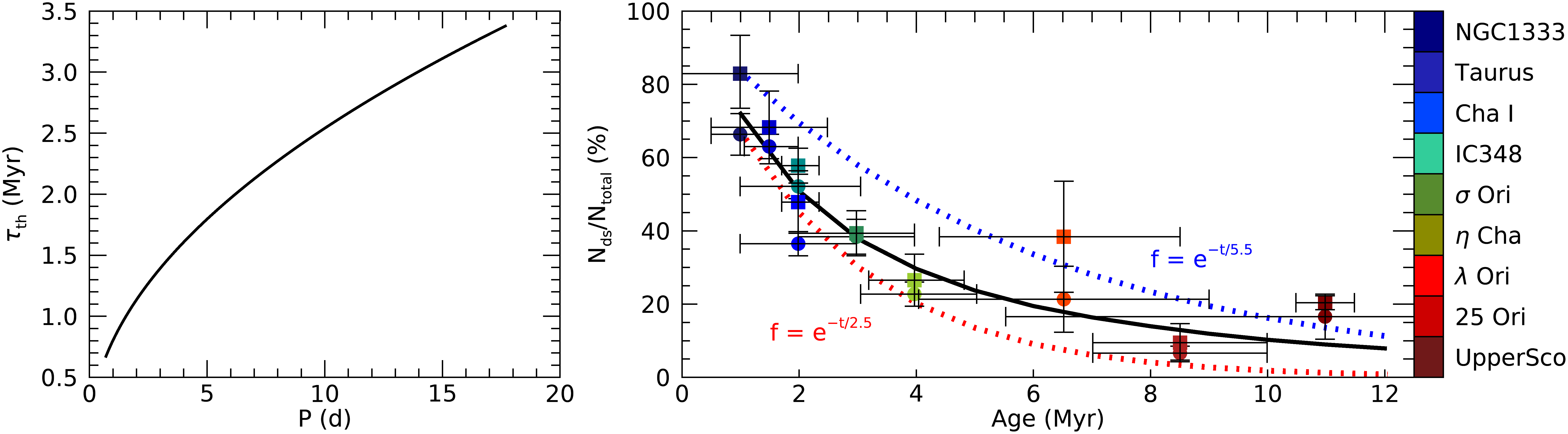
Figure 1: Left panel: the parameter $\tau_{\mathrm{th}}$ as a function of rotational period. Right panel: disk fraction as a function of cluster age superimposed on data for nine young nearby clusters, associations and groups shown as colored dots taken from Ribas et al. (2014, circles), Hernández et al. (2007, 2008, squares). The cluster ages were taken from Ribas et al. (2014). The dotted lines are exponential decay laws expected from disk e-folding times 2.5 Myr (red line) and 5.5 Myr (blue line). Both figures are obtained for $\overline{P}=7.5$ d.

Vasconcelos & Bouvier (2015, hereafter Paper I) created a synthetic cluster of rotating solar mass stars (0.3 - 1.0 M_⊙). The paper’s goal was to reproduce the rotational period distributions seen in clusters younger than 20 Myr, particularly, the ONC, NGC 2264 and h Per. For this purpose, the stellar angular velocities were evolved taking into account only the spin up due to PMS contraction and without considering any angular momentum loss. In Paper I, the stellar population was divided in disk and diskless stars and only the latter had their angular velocities evolved. This simple approach was successful in reproducing qualitative aspects of the ONC, NGC 2264 and Cyg OB2 stellar periods, the relation between disk fraction and mass accretion rate and rotational period but failed to capture the striking bimodality of h Per. In Vasconcelos & Bouvier (2017, Paper II) the same kind of simulations were performed but in the brown dwarf and very low mass regime. The results show that the rotational behavior of these low mass objects is different from their higher mass counterparts. In this case, the disk locking is not so necessary in order to reproduce the observed period distributions. The conclusion was that these lower mass objects should rotate faster than solar mass stars.

In this paper, we want to extend Paper I’s simulations to include angular momentum loss through stellar magnetized winds and the core-envelope decoupling in order to investigate the rotational pattern of clusters as old as the 550 Myr old M37. There are some previous similar works. Spada et al. (2011) generated a synthetic population of solar mass stars and evolved it from 2 Myr to 4.5 Gyr considering disk locking, core-envelope coupling and angular moment loss by a wind. They focused in obtaining prescriptions for the core-envelope coupling timescale and optimized parameters and compared their synthetic populations to clusters of similar ages. Gondoin (2017) also constructed a synthetic population at 5 Myr based on the period distribution of NGC 2362 consisting of 1000 0.7 - 1.1 M_⊙ stars with 0.3 d $\leq$ P $\leq$ 30 d. No disk locking was imposed and a constant value core-envelope coupling timescale was assumed and also an enhanced angular momentum loss attached to a Rossby number interval. According to the author, this “catastrophic" braking will generate bimodal period distributions from 20 Myr to 600 Myr that are in agreement with the observations. Coker et al. (2016) used YREC stellar code (Demarque et al., 2008) that solves 1D equations of the stellar structure taking into account structural changes due to rotation, the presence of disks and winds and internal angular momentum transport. They evolved the period distribution of a population of 0.3 - 0.7 M_⊙ stars from 1 Myr to 13 Myr and then to 550 Myr. Initially they construct a distribution based on the ONC periods of disk and diskless stars taken from Rebull et al. (2006) data. The distributions are evolved from 1 Myr to 13 Myr and compared to h Per data. The authors concluded that they cannot reproduce the fast h Per rotators peak. After, they evolved a new distribution obtained from h Per data by Moraux et al. (2013) from 13 Myr to 550 Myr. After comparing their results to the Pleiades (Hartman et al., 2010; Covey et al., 2016) and M37 (Hartman et al., 2009) data they concluded that they can reproduce the slow rotators but not the fast rotators of these distributions. Lanzafame & Spada (2015) constructed two-zone models testing different wind braking prescriptions: i) the Kawaler (1988) law as modified by Chaboyer et al. (1995); ii) the Kawaler (1988) law with the mass dependence suggested by Barnes & Kim (2010) and Barnes (2010); iii) the braking law proposed by Gallet & Bouvier (2013) and iv) the braking law by Matt et al. (2015). They assume the same constant rotational period and disk lifetimes for the stars independent of their mass for all models. They constrain the set of free parameters necessary to describe the slow rotator sequence of clusters from 0.1 to 2.5 Gyr for the mass range 0.85 - 1.1 M_⊙ using a Monte Carlo Markov Chain method. Their results show that in order to reproduce the observations the coupling time scale related to the angular momentum exchange between the stellar radiative interior and the convective envelope should vary with the mass. Concerning the wind prescriptions, they conclude that all models reproduce well the observations but prescription ii) is better. In order to reproduce the slow rotator sequence of the main sequence open clusters Praesepe (700 Myr) and NGC 6811 (1 Gyr), Spada & Lanzafame (2020) used the Lanzafame & Spada (2015) model with parameters adjusted to better reproduce the clusters. They adopted the wind braking law with Barnes & Kim (2010) mass and Kawaler (1988) $\omega_{\mathrm{env}}^{3}$ dependencies (wind prescription ii above). The rotational coupling timescale shows a stronger mass dependency compared to what was obtained by Lanzafame & Spada (2015). They show that this is essential to capture the rotational behavior of 0.5 - 0.8 M_⊙ stars which present almost the same rotational periods in the two clusters. They conclude that at this mass range, resurfacing of angular momentum causes an apparent reduction of NGC 6811 spinning down. In this sense, the evolution of the rotational distribution of older clusters is not only due to the wind loss but depends also on internal exchanges of angular momentum.

In this work, we will investigate if we can reproduce the rotational pattern of some clusters using disk locking, angular momentum loss by a magnetized wind and internal exchange of angular momentum. Differently from these earlier works, the disk lifetime will be a function of the initial rotation period and we will consider the wind angular momentum loss given by Gallet & Bouvier (2013, 2015). We will experiment different disk timescales and initial conditions. The models will be compared to the observations by means of the statistical Kolmogorov-Smirnov test. In Section 2 we present the equations and the numerical setup of our simulations. In Section 2.1 we discuss our standard model, M1. Variations upon this model will be present in Section 2.2 and its subsections. Finally in Section 3 we draw our conclusions.

2 The numerical setup

Our numerical setup is very similar to that of Paper I. We start our simulations at 1 Myr creating initial distributions for the rotational period and the mass accretion rate of the population. The rotational period distribution is a bimodal truncated Gaussian. The distribution is limited to 0.7 and 18.5 days. The mass accretion rate initial distributions are log-normal functions with a mean equal to the logarithm of $10^{-8}$ (M_∗/M${}_{\odot})^{1.4}$ M_⊙ yr^-1 and a standard deviation $\sigma=0.8$. The mass values considered in this work are equal to 0.5, 0.8 and 1.0 M_⊙ The number of stars in each mass bin is calculated according to the canonical IMF by Kroupa et al. (2013). Other stellar mass values and distributions will be investigated in Section 2.2.4. The total number of stars is around 50,000. The mass accretion rate is evolved at each time step and varies with t^-1.5 (Hartmann et al., 1998).

Until 12 Myr, we consider the disk locking hypothesis and the angular velocity (or period) of disk stars is constant although as can be seen in Fig. 1, at this age, most of the stars no longer have disks. According to the observations, the expected disk lifetime is shorter than 12 Myr. With our hypothesis stars with long living disks will not have much time to spin up significantly (see Fig. 4). The presence or absence of the disk is determined by the comparison of the stellar mass accretion rate to a threshold which is given by,

$$\dot{\mathrm{M}}_{\mathrm{acc,th}}=10^{-8}\left(2.2\sqrt{\frac{P_{0}}{\overline{P}}}\right)^{-1.5}(M_{\ast}/M_{\odot})^{1.4}.$$ (1)

It depends on the initial stellar period, $P_{0}$, on $\overline{P}$, a free parameter, and on stellar mass. In Paper I we have shown that at an age of 2.2 Myr, half of the stars have lost their disks. Here, the mass accretion rate threshold depends on the stellar initial rotating rates as suggested by Gallet & Bouvier (2013, 2015). Slowly rotating stars, for example, will have smaller mass accretion rate thresholds. A small $\dot{\mathrm{M}}_{\mathrm{acc,th}}$ value implies longer lasting disks, since it will take longer for the mass accretion rate to reach the threshold. One can define a time scale $\tau_{\mathrm{th}}$ given by the expression inside the parentheses in Eq. 1. In the left panel of Fig. 1, we show $\tau_{\mathrm{th}}$ as a function of the rotational period considering $\overline{P}=7.5$ d. The longer $\overline{P}$ the shorter $\tau_{\mathrm{th}}$. One can note that the maximum $\tau_{\mathrm{th}}$ value obtained for $\overline{P}=7.5$ d is about 3.5 Myr. When analyzing disk fractions as a function of cluster age (right panel of Fig. 1), we note that this $\overline{P}$ value gives a disk fraction which is in agreement with most of the observed values and between two exponential curves with e-folding times equal to 2.5 Myr and 5.5 Myr. Equation (1) for the parameter $\tau_{\mathrm{th}}$ provides a range of mass accretion rate thresholds instead of just one value per mass. If $\dot{M}_{\mathrm{acc}}(t)\leq\dot{M}_{\mathrm{acc,th}}(M_{\ast},P_{0},\overline{P})$ the star loses its disk. Then, the angular velocity is evolved. After 12 Myr, all stars will be considered diskless, even if their mass accretion rates are above $\dot{M}_{\mathrm{acc,th}}$.

PMS stars can lose angular momentum through a stellar magnetic wind. For the mass interval considered in this work, the stars will develop a radiative core. In this case, it is expected some kind of exchange of angular momentum between the core and the envelope. There is no definitive mechanism to explain this exchange but the best ones are related to internal gravity waves, hydrodynamical instabilities and magnetic fields (for a short review, see Bouvier et al., 2014). We implement the so-called double zone model in which both the core and the envelope are considered solid bodies that interact at a rate given by a free parameter, the core-envelope coupling timescale, $\tau_{ce}$ (MacGregor & Brenner, 1991; Irwin et al., 2007). The greater $\tau_{ce}$, the weaker the core-envelope interaction. It means that a smaller amount of angular momentum will be exchanged by the core and the envelope. The equations for the evolution of the envelope and core angular velocities ($\omega_{env}$ and $\omega_{core}$, respectively) for diskless stars are given by,

$$\begin{split}\frac{d\omega_{env}}{dt}=&\frac{1}{I_{env}}\frac{\Delta J}{\tau_{ce}}-\frac{2}{3}\frac{R^{2}_{core}}{I_{env}}\omega_{env}\frac{dM_{core}}{dt}-\frac{\omega_{env}}{I_{env}}\frac{dI_{env}}{dt}\\ \\ -&\frac{w_{env}}{J_{env}}\dot{J}_{\mathrm{wind}},\end{split}$$ (2)

$$\begin{split}\frac{d\omega_{core}}{dt}=&-\frac{1}{I_{core}}\frac{\Delta J}{\tau_{ce}}+\frac{2}{3}\frac{R^{2}_{core}}{I_{core}}\omega_{env}\frac{dM_{core}}{dt}\\ \\ -&\frac{\omega_{core}}{I_{core}}\frac{dI_{core}}{dt},\end{split}$$ (3)

with,

$$\Delta J=\frac{I_{env}J_{core}-I_{core}J_{env}}{I_{env}+I_{core}},$$ (4)

Table 1: Core-envelope coupling timescales

Mass (M⊙)	Slow	Medium	Fast
	Rotators (Myr)
0.5	500	300	150
0.8	80	80	15
1.0	30	28	10

$$I_{\mathrm{core,env}}=k_{\mathrm{core,env}}^{2}M_{\ast}R_{\ast}^{2},$$ (5)

In the equations above, the symbols have their usual meanings, namely, the moments of inertia $I$ (for the core and envelope, $I_{core}$ and $I_{env}$, respectively), angular velocity $\omega$ (for the core and envelope, $\omega_{core}$ and $\omega_{env}$), the core radius ($R_{core}$), the angular momentum $J$ (for the envelope and the core, $J_{env}$ and $J_{core}$), and the mass $M$ (for the star and for the core, $M_{\ast}$ and $M_{core}$). $\dot{J}_{\mathrm{wind}}$ is the torque due to the magnetized stellar wind and $k_{\mathrm{core,env}}$ is the gyration radius for the core or the envelope. They were calculated by Baraffe et al. (1998) using the expressions:

$$k_{\mathrm{core,env}}=\sqrt{\frac{I^{\mathrm{{mod}}}_{\mathrm{{core,env}}}}{M_{\ast}R_{\ast}^{2}}},$$ (6)

with,

$$I^{\mathrm{{mod}}}_{\mathrm{{core,env}}}=\frac{2}{3}\int r^{2}dm.$$ (7)

The integral in the equation above is calculated over the mass of the convective regions and the regions below. The variable $dm$ is the mass of a thin shell of radius $r$ inside a spherical star.

Since we are considering the core and the envelope as bodies in solid rotation, the equations of angular velocity evolution have terms related to angular momentum variation (torques) and terms related to the stellar contraction (i.e. to the evolution of the moment of inertia). These last ones are the 3^rd terms in equation (2) and equation (3). In the PMS, due to contraction, the star is spun up since its total moment of inertia decreases. When the radiative core develops, the moment of inertia of the core increases but the moment of inertia of the envelope decreases and so these terms contribute to decrease the core angular velocity $\omega_{\mathrm{core}}$ but to increase $\omega_{\mathrm{env}}$. This imbalance stabilizes when the star reaches the main sequence. The first terms in equation (2) and equation (3) are torque terms related to the core-envelope exchange of angular momentum (MacGregor & Brenner, 1991). They can be positive or negative depending on the relation between $\omega_{\mathrm{core}}$ and $\omega_{\mathrm{env}}$ and they always act to establish uniform internal rotation. Due to the mass and radius increase of the core, initially $\omega_{\mathrm{core}}>\omega_{\mathrm{env}}$ and so there is a transfer of angular momentum to the envelope which will occur over the $\tau_{\mathrm{ce}}$ timescale. The second terms are torque terms due to the mass increase of the radiative core (Allain, 1998). Finally, the last term in equation (2) is the torque due to the the magnetized stellar wind. Stellar parameters are taken from Baraffe et al. (1998)’s models.This stellar evolutionary model neglects the effects of accretion (see, e.g., Baraffe & Chabrier, 2010) and rotation (e.g., Landin et al., 2016; Amard et al., 2019). All terms related to the development of the core have no effect until around 3 - 4 Myr for 0.8 - 1 M_⊙ stars and later, around 13 Myr, for 0.5 M_⊙ stars. Our models use the angular momentum loss due to a magnetized wind given by Gallet & Bouvier (2015) in the form,

$$\Gamma_{\mathrm{wind}}=\omega_{\ast}\dot{M}_{\mathrm{wind}}r_{\mathrm{A}}^{2},$$ (8)

where $\omega_{\ast}$ is the stellar angular velocity, $\dot{M}_{\mathrm{wind}}$ is the mass loss rate given by the numerical simulations of Cranmer & Saar (2011) and modified by Gallet & Bouvier (2013) and $r_{\mathrm{A}}$ is the average value of the Alfvén radius given by Matt et al. (2012).

We consider three models, M1, M2 and M3. Models M1 and M2 share the same initial period distributions for disk and diskless stars. For disk stars, the distribution has a mean equal to $\overline{P}_{\mathrm{d}}=7.0$ days and a dispersion of $\sigma_{\mathrm{d}}=3.0$ days. For diskless stars, we adopt a distribution with $\overline{P}_{\mathrm{dl}}=2.0$ days and $\sigma_{\mathrm{dl}}=4.0$ days. All models use the same core-envelope coupling timescale $\tau_{\mathrm{ce}}$ values (Gallet & Bouvier, 2015), which are shown in Table 1. Models M1 and M2 have different $\overline{P}$, equal to 7.5 days and 2.0 days, respectively, which normalizes the mass accretion rate threshold (equation 1). Model M3 begins at 13 Myr with a period distribution taken from the observational period distribution of h Per (Moraux et al., 2013). We also examine the effect that other mass values and distributions have on model M1 in Section 2.2.4. Torques due to the magnetized wind were calculated for a grid of initial periods from 0.05 to 45 days using Gallet & Bouvier (2015) prescription. The values for the actual period distributions were then obtained by interpolation. The values necessary to calculate the other torque terms were taken or calculated from Baraffe et al. (1998) stellar models for each one of the masses. The core-envelope coupling timescales for models M1, M2 and M3 have the same values as those of Gallet & Bouvier (2015), considering their definition of slow, median and fast rotators. The corresponding values for the intermediate masses used in section 2.2.4 have all been obtained by interpolation, except the stellar parameters for which we have the values from Baraffe et al. (1998) tables.

Table 2: Selection criteria for the observational samples.

Cluster	Age (Myr)	Age Ref.	Mass/Spt/Color index range	Disk?a	Nb	Ref.
ONC	2	Mayne & Naylor (2008)	K4.5 - M0	[3.6] - [8.0] $>$ 0.7	68	Cieza & Baliber (2007)
ONC	2	"	K4.5 - M0	Class/Accreting	45	Davies et al. (2014)
Cyg OB2c	5	Wright et al. (2010)	0.5 - 1.0 M⊙	0 - 1	258	Roquette et al. (2017)
NGC 2362	4-5	Mayne & Naylor (2008)	0.5 - 1.0 M⊙	-	88	Irwin et al. (2008)
U Sco	11	Pecaut et al. (2012)	$2.0\leq(V-K_{s})_{0}\leq 4.1$	-	144	Rebull et al. (2018)
h Per	13	Mayne & Naylor (2008)	0.5 - 1.0 M⊙	-	219	Moraux et al. (2013)
Pleiades	125	Stauffer et al. (1998)	0.5 - 1.0 M⊙	-	184	Rebull et al. (2016), Lodieu et al. (2019)
M37	550	Hartman et al. (2008)	$0.76\leq(V-I)\leq 2.0$	-	366	Hartman et al. (2009)
a Disk selection criteria as found in the respective references.
b Number of stars after the application of the selection criteria.
c Stars with periods greater than 2 days. See text for details.

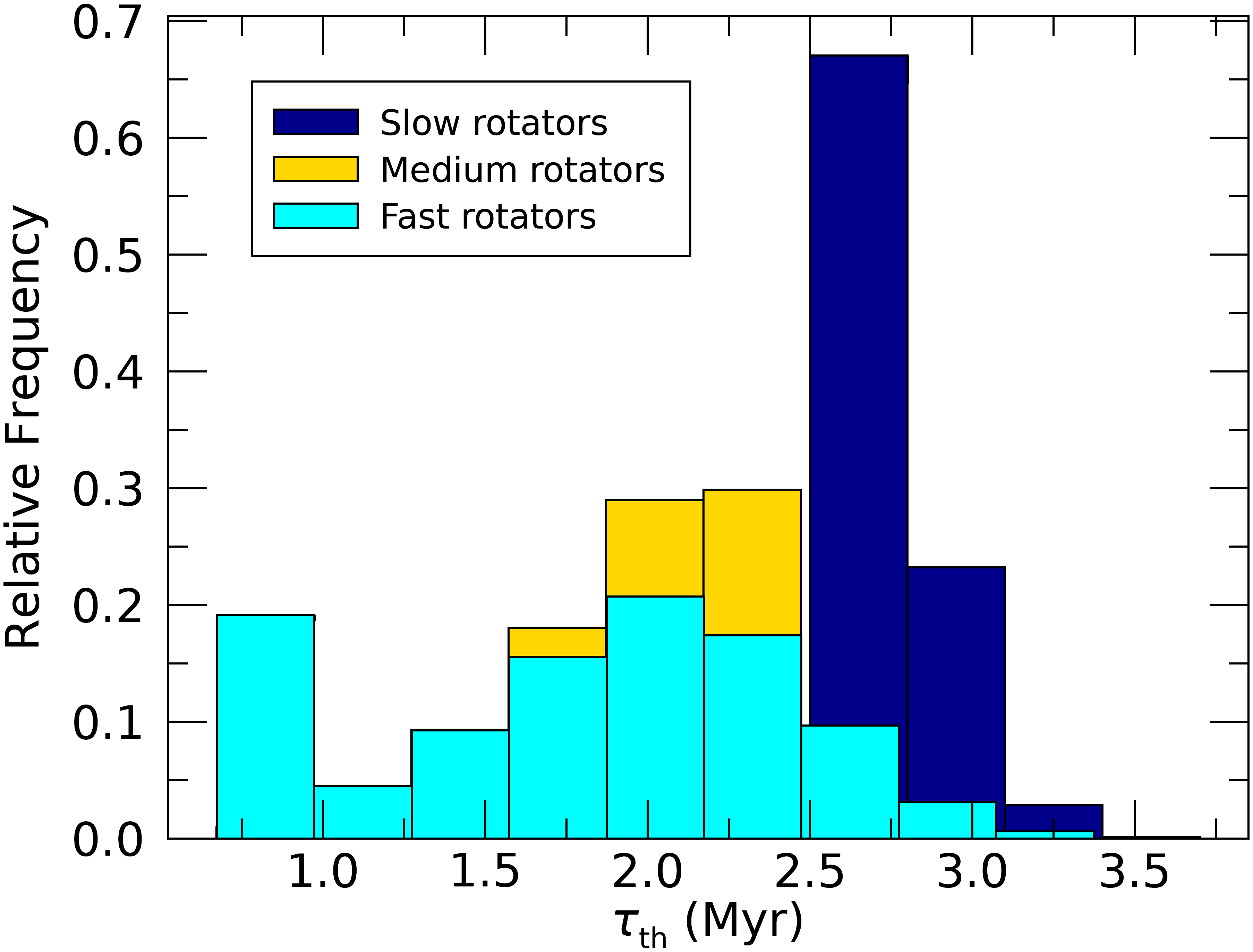
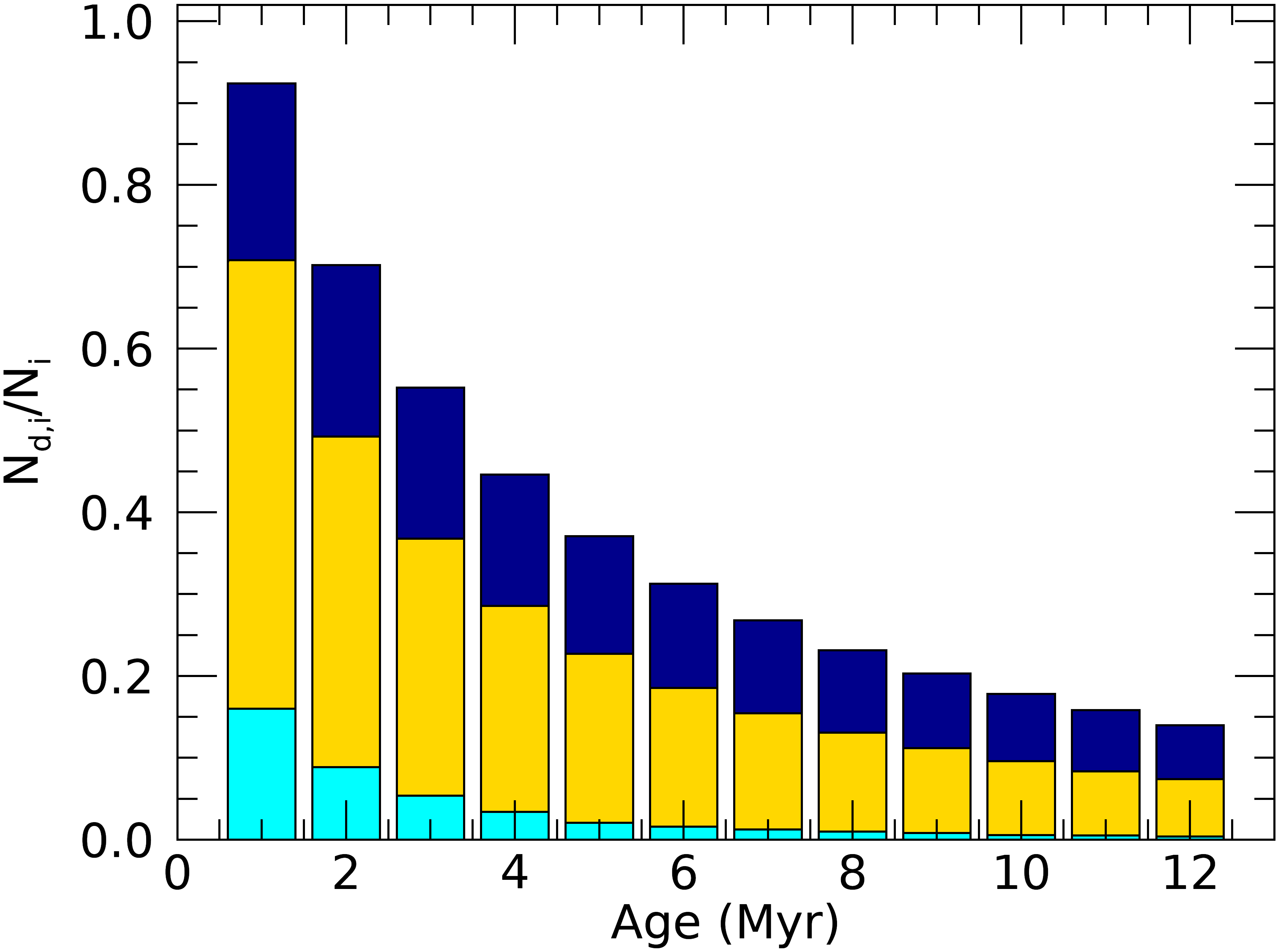
Figure 2: Top panel: Distribution of the parameter $\tau_{\mathrm{th}}$ for slow, median and fast rotators obtained for model M1. Bottom panel: Distribution of disk stars. Slow rotators are represented by dark blue bars; median rotators by yellow bars and fast rotators by light blue bars.

The equations are evolved from 1 to 550 Myr for models M1 and M2 and from 13 to 550 Myr for model M3. All the results are compared to data of the ONC (Davies et al., 2014; Cieza & Baliber, 2007), Cyg OB2 (Roquette et al., 2017), Upper Sco (Rebull et al., 2018), h Per (Moraux et al., 2013), the Pleiades (Rebull et al., 2016; Lodieu et al., 2019) and M37 (Hartman et al., 2009). The selection criteria applied to the observational data are shown in Table 2. The Cyg OB2 sample only contains stars with periods longer than 2 days because they are free from contaminants (for more details, see Roquette et al., 2017). For the Pleiades, we have cross matched the samples from Lodieu et al. (2019) and Rebull et al. (2016). In this work, we adopt solar metallicity stellar evolutionary models (Baraffe et al., 1998). Most of the samples analyzed here have solar metallicity. The ONC (Padgett, 1996; D’Orazi et al., 2009; Biazzo et al., 2011), U Sco (Viana Almeida et al., 2009) and the Pleiades (Takeda et al., 2017) present solar metallicity. Although Cyg OB2 does not have determinations of abundance, Wright et al. (2010), Guarcello et al. (2013) and Roquette et al. (2017) all use solar metallicity stellar models. Berlanas et al. (2018) find no evidence of self-enrichment in Cyg OB2. There are some works showing that the metallicity of h Per is sub solar (Z = 0.01 - Southworth et al., 2004; Tamajo et al., 2011). However, Dufton et al. (1990) and Smartt & Rolleston (1997) obtained solar abundances for the same cluster. For M37 (NGC2099), Casamiquela et al. (2017) obtained Z = + 0.08 while Netopil et al. (2016) obtained Z = + 0.02. There are several uncertainties related to age determination particularly for young clusters (see, for example Soderblom et al., 2014). The ages and corresponding references adopted in this work are shown in the 2^nd and 3^rd columns of Table 2. For NGC2362, Mayne & Naylor (2008) suggest an age range between 4 and 5 Myr. We choose the age of 5 Myr because this is in better agreement with our models. For Cyg OB2, Wright et al. (2015) observe an age spread consistent with an extended stellar formation phase of 6 Myr with a peak between 4 - 5 Myr. We assume an age of 5 Myr for the cluster, as suggested by Wright et al. (2010). Among the clusters studied in this work, the age attributed to U Sco exhibits the greatest variation, from 5 Myr (Slesnick et al., 2008; Herczeg & Hillenbrand, 2015) to 11 Myr (Pecaut et al., 2012). Rebull et al. (2018) adopt 8 Myr for it but an 11 Myr old rotational period distribution returns a better value in the KS tests performed in this work.

2.1 Model M1

In the top panel of Fig. 2, we show the distribution of the parameter $\tau_{\mathrm{th}}$ obtained using model M1. We define three classes of rotators, following Gallet & Bouvier (2013): fast rotators, with $P\leq 1.4\;\mathrm{d}$; median rotators, with $1.4\;\mathrm{d}\leq P\leq 10\;\mathrm{d}$ and slow rotators, with $P>10\;\mathrm{d}$. In this figure, there are two peaks for fast rotators, one at $\boldmath{\tau_{\mathrm{th}}}$ equal to 0.67-0.97 Myr and the other at 1.87-2.17 Myr both shorter than the peak for median rotators which is between 2.17 - 2.47 Myr. Most of slow rotators present $\tau_{\mathrm{th}}$ values around $\sim 2.48-2.78$ Myr with a maximum value around 3.4 Myr. As discussed in Section 2, higher $\tau_{\mathrm{th}}$ values imply lower $\dot{\mathrm{M}}_{\mathrm{acc,th}}$. Because of this, most of the fast rotators will have short living disks while median and slow rotators will have longer living disks. This can be seen at the bottom panel of Fig. 2 where the distribution of disk stars is shown for slow, median and fast rotators. At 1 Myr, only 15% of fast rotators have disks against more than 90% of the slow rotators. Only at 12 Myr the fraction of disk slow rotators falls below the initial fraction of disk fast rotators. At 12 Myr, all fast rotators are diskless while we can find around 13% and 7% of disk bearing stars among slow and median rotators, respectively. In spite of that, after this age, all stars will be considered diskless and their periods will be evolved following equation (2) and equation (3).

Core-envelope coupling timescale values, $\tau_{\mathrm{ce}}$, are shown in Table 1. The values were taken from Gallet & Bouvier (2015). This timescale sets the rate of angular momentum transfer from the core to the envelope. One can note that it depends on mass and initial rotation rate. With these values, 0.5 M_⊙ stars will take much longer to reach uniform internal rotation than 1.0 M_⊙ stars.

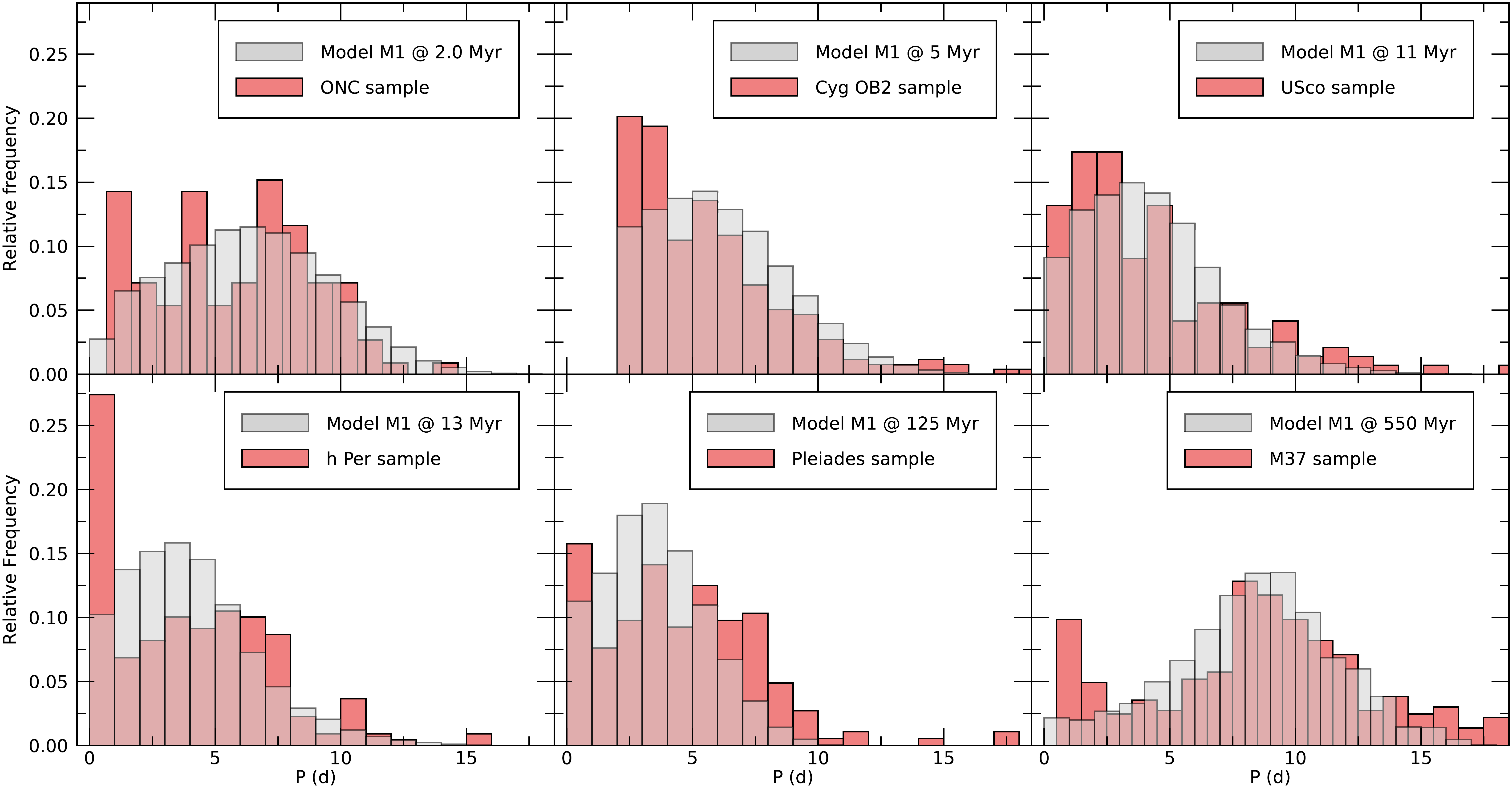
Figure 3: Period distributions of model M1 at different ages (grey bars) and the observational data (light coral bars). Top row: (left panel) model at 2.0 Myr superimposed to ONC period distribution; (middle panel) model at 5 Myr superimposed to Cyg OB2 data and (right panel) model at 11 Myr over U Sco data. Bottom row: (left panel) model at 13 Myr and h Per data; (middle panel) model at 125 Myr and Pleiades data; (right panel) model at 550 Myr and M37 data.

For model M1, all the initial parameters have been chosen in order to maximize the statistical compatibility with the ONC period distributions. In the top left panel of Fig. 3 we show the period distribution at 2.0 Myr obtained with this model (grey bars) superimposed to observational ONC data (coral bars) which is the result of the combination of the samples by Cieza & Baliber (2007) and Davies et al. (2014). In the same figure we present more evolved distributions. In the top row, we show the distribution at 5 Myr compared to Cyg OB2 and the distribution at 11 Myr compared to U Sco data. At the bottom row we show the distributions at 13 Myr, 125 Myr and 550 Myr superimposed to h Per, Pleiades and M37 samples, respectively. We see that the theoretical distributions move to shorter periods increasing the number of faster rotators from 2 Myr to 125 Myr. In fact, the peak of the distribution moves from 5-8 days at 2 Myr to 3-4 days at 13 Myr and 125 Myr. However, the peak moves back to 8-10 days at 550 Myr which means that the number of slow rotators increases at later ages, as can be seen in Fig. 4. Analyzing this figure, we note that after the constant evolution at the disk phase, the stars experience a strong spin up during the PMS. After that, the loss of angular momentum due to the magnetized stellar wind causes a strong braking and this moves the distribution to longer periods (smaller angular velocities values) at 550 Myr. A very small fraction of model M1 stars reach breakup velocities. They represent at most 1% of 1.0 M_⊙ and 0.3% of 0.8 M_⊙ stars. These fractions decrease to 0.4% of 1.0 M_⊙ and 0.2% of 0.8 M_⊙ stars in model M2 (section 2.2.1) and to 0.4% of the stars in the mass range 0.6 - 1.0 M_⊙ in the last model considered (section 2.2.3). None of the stars of model M3 reach or exceeds the critical limit. There is no attempt to fix or to remove these stars from the simulations because the number of critical rotators is not high enough to alter the conclusions of our study. In Figure 4, we have included three dash-dotted green lines showing the breakup velocities and two solid green lines showing the angular velocities of the 0.8 M_⊙ and 1.0 M_⊙ stars which present the most extreme rotation rates. The fastest rotator is a 1.0 M_⊙ star that achieves at 28 Myr an angular velocity that is 27% higher than the expected breakup angular velocity at this age followed by a 0.8 M_⊙ star that rotates at a rate 12% higher than the break up at 48 Myr.

Table 3: K-S tests results comparing the simulated period distributions for all stars and the observational period distributions.

Cluster	$D_{\mathrm{crit}}$	$D_{\mathrm{M1}}$	$D_{\mathrm{M2}}$	$D_{\mathrm{M3}}$
ONC	0.128	0.10	0.15	-
Cyg OB2	0.084	0.16	0.16	-
NGC 2362	0.14	0.11	0.12	-
U Sco	0.11	0.11	0.21	-
h Per	0.092	0.18	0.22	0.01
Pleiades	0.096	0.22	0.14	0.17
M37	0.071	0.097	0.13	0.094

In order to compare the samples, we apply a two-sample Kolmogorov-Smirnov (K-S) test to the simulated and observational period distributions. Through this test we calculate the maximal difference $D_{n,m}$ between two cumulative functions of size $n$ and $m$ and compare it to a critical value $D_{\mathrm{crit}}$ that depends on the number of objects on the samples and the significance level, taken here to be equal to 0.05. If $D_{n,m}<D_{\mathrm{crit}}$, the simulated and observational samples can be said to be derived from the same population. In Table 3, we show the K-S statistics expressed by $D_{\mathrm{crit}}$ and by the $D$ values obtained for models M1, M2 and M3, respectively. From this table we note the ONC sample and the simulated period distribution at 2 Myr for model M1 are derived from the same population. We arrive at the same conclusion for NGC 2362 and U Sco. For all the other clusters, the comparison indicates that the agreement is not significant at the 0.05 level. Interestingly, while there is no similarity with Cyg OB2 data, model M1 and NGC 2362 can be said to derive from the same population, although both clusters have the same age. When we look at the two distributions separately (Fig. 5) we note that Cyg OB2 has more fast rotating stars than NGC 2362 which has relatively more slowly rotating ones. However, Cyg OB2 has two stars rotating slowly than 30 days while the maximum period found in NGC 2362 is around 27 days. Littlefair et al. (2010) also found that 5 Myr old Cep OB3b presents a different rotation pattern when compared to NGC 2362. Its period distribution can also be seen in Fig. 5. The 3 clusters present different period distributions, although Cyg OB2 and CepOB3 are more similar, with more fast rotating stars than NGC 2362. The same is true for U SCo and h Per, which are about the same age but exhibit quite different rotational period distributions. As Littlefair et al. (2010) and Coker et al. (2016) pointed out there seems to exist differences among clusters of same age due perhaps to environmental causes. Recent papers (Concha-Ramírez et al., 2021; Guarcello et al., 2021; Roquette et al., 2021) explore different mechanisms that can influence the evolution of disks depending on the cluster’s environment. A shorter disk lifetime, for example, can have an impact on the rotation pattern observed in coeval clusters.

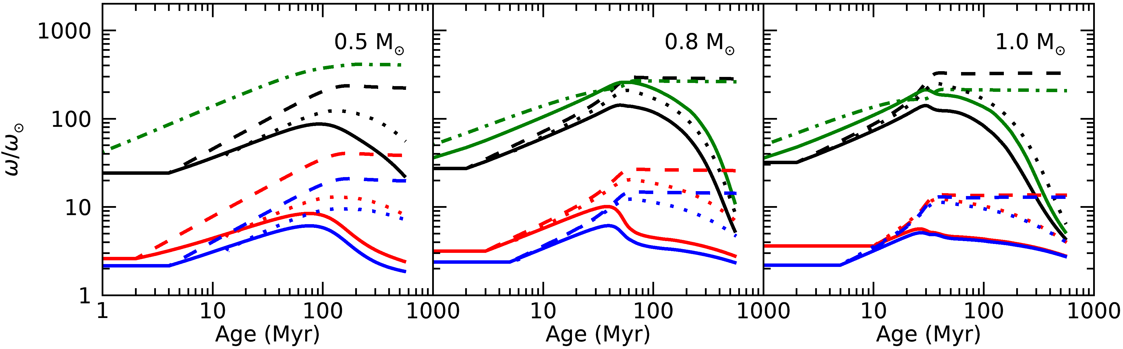
Figure 4: Angular velocity evolution as a function of age. Blue, red and black curves show the evolution of three randomly selected stars at each mass bin. The three chosen stars have disks at 1 Myr and are slow (blue), medium (red) and fast (black) rotators, respectively. Solid lines show the angular velocity of the convective envelope while dotted lines show the angular velocity of the radiative core. Dashed lines trace the evolution of angular velocity considering angular momentum conservation after disk loss following Paper I’s model M2. Green dash-dotted lines show the breakup limit and solid green lines show the most extreme rotators with 0.8 M_⊙ (middle panel) and 1.0 M_⊙ (right panel).

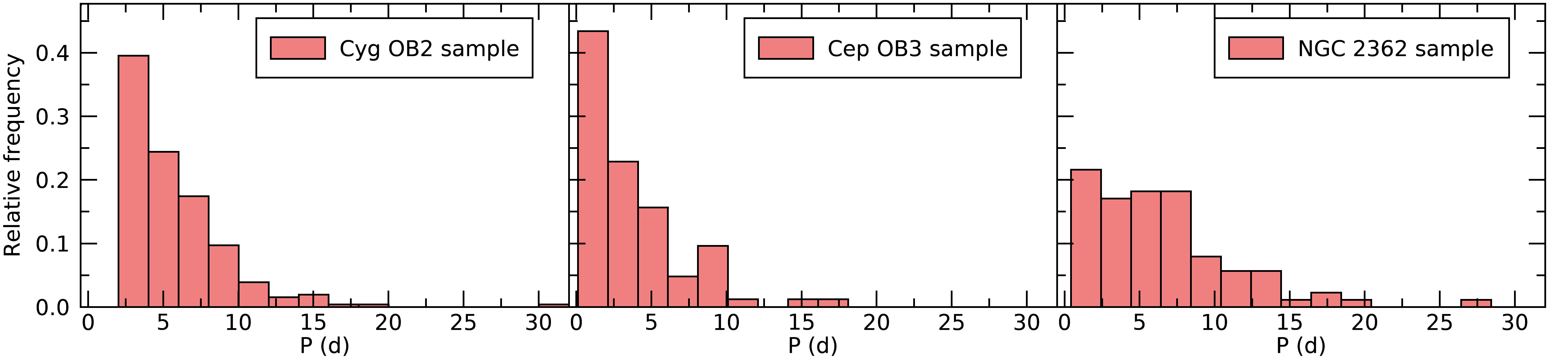
Figure 5: Period distributions of three 5 Myr old clusters: CygOB2 (left panel), CepOB3 (middle panel) and NGC 2362 (right panel).

The comparisons between model M1 period distributions and the observational samples older than U Sco show worse results. At 13 Myr the agreement with the h Per sample is poor. The observational sample is bimodal while the model is not. The number of the fastest rotators ($\sim$ 1.0 day) and stars within the period range of 6-8 days is smaller than observed. On the other hand, there is an excess of stars rotating at periods between 1-6 days. Indeed, the K-S statistic for this case gives a maximal difference D_n,m which is two times greater than the critical one. The agreement with the Pleiades is not better. The same deficiencies observed for the h Per sample are seen here, but displaced to slightly shorter periods. The comparison of model M1 at 550 Myr with M37 data is better but we cannot say that the samples are drawn from the same population. There is still a lack of fast rotators and of stars with periods longer than 14 days and an excess of stars with periods between 4 and 11 days.

We can note the effects the introduction of the mechanisms of angular momentum variation produced in our models looking at Figure 4, where dashed lines trace the evolution of the angular velocity of randomly chosen stars considering angular momentum conservation similarly to Paper I’s model M2. The curves show no variation after an initial steep increase, just after the disk loss, when the star arrives at the ZAMS. Statistical comparisons of period distributions obtained under this J constant condition with the observational samples of stellar clusters younger than 13 Myr give worse results than those we have obtained with model M1: only at 2.0 Myr model and observational distributions can be said to be derived from the same population. Even before the arrival at the main sequence the angular momentum internal re-distribution and loss play an important role in determining the rotational behavior of a star.

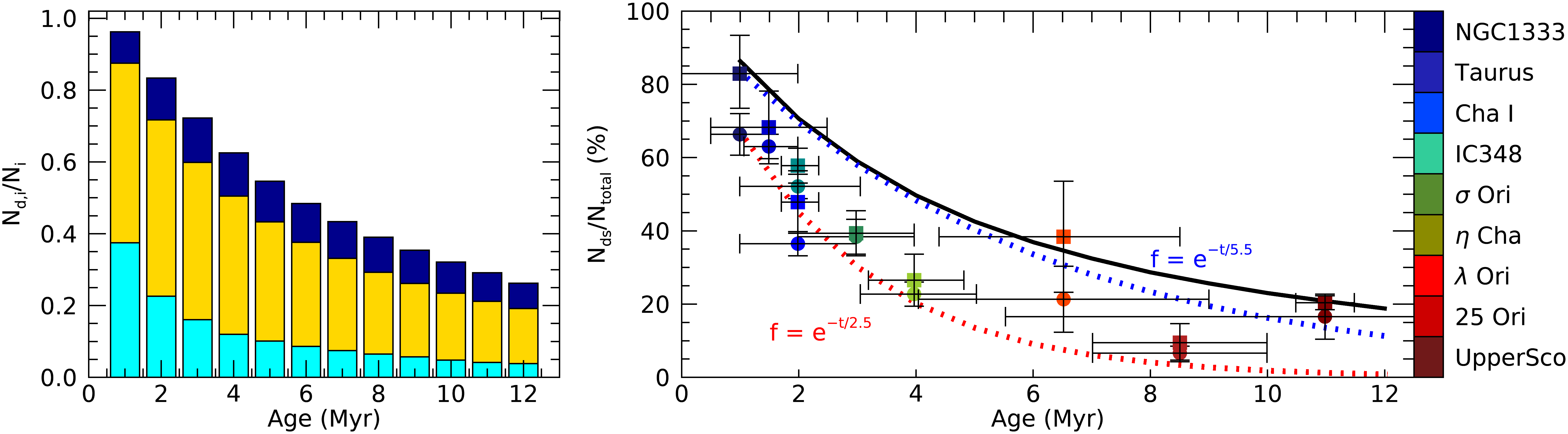
Figure 6: Left panel: Distribution of disk stars for slow (dark blue), median (yellow) and fast (light blue) rotators for model M2. Right panel: disk fraction as a function of age for the same model; lines and symbols are the same of those seen at the right panel of Fig. 1. Results obtained using $\overline{P}=2.0$ d.

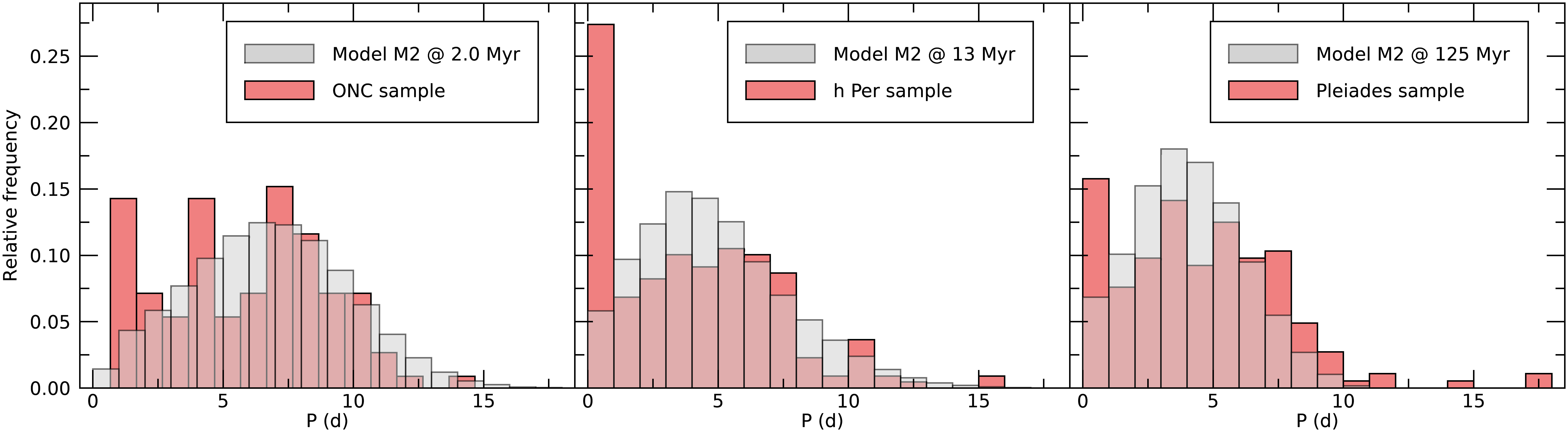
Figure 7: Same as Fig. 3 but for model M2.

2.2 Exploring other parameters - models M2, M3 and other initial mass distributions

In order to try to understand the impact of some key parameters on the simulations, we will explore a different set of values. We will change the parameter $\overline{P}$ and the initial conditions. Also, we will consider initial mass distributions based on the samples studied.

2.2.1 Model M2

Since model M1 was not able to explain the evolution of the rotational period distributions from the PMS to MS phases we decided to explore other parameters. In model M2, we change the value of $\overline{P}$ to 2.0 days. This change will increase the maximum $\tau_{\mathrm{th}}$ value from 3.4 days to 7 days causing a reduction of the mass accretion rate threshold values, increasing the disk fractions of the rotators (left panel of Fig. 6) and the total disk fraction that now falls off more slowly than previously seen in model M1 (Fig. 6, right panel).

Stars with longer living disks will maintain their initial rotational rates for a longer time (Gallet & Bouvier, 2015). This will increase the number of slower rotators which is what effectively happened as can be seen in Fig. 7 where period distributions at 2.0 Myr, 13 Myr and 125 Myr are shown in comparison with data from the ONC, h Per and the Pleiades. When we compare this figure to Fig. 3, at 2 Myr, the number of stars with $P\leq 5$ days has decreased while it has increased for 5 d $<P\leq 12$ d. At 13 Myr and 125 Myr, one can observe the same behavior but at different intervals: at both ages, the number of stars decreases in comparison with the standard model until P = 4 d; at 13 Myr, it increases over the range from 6 d to 15 d; at 125 Myr over the range from 5.0 d to 11 d. The 4^th column of Table 3 indicates that the maximal difference increased for almost all clusters which means that the agreement among the M2 simulated period distributions and the observational clusters is now poorer compared to that of model M1, except for Cyg OB2 and the Pleiades and also for NGC 2362, because the D_n,m increase was very small in this case. For Cyg OB2, the maximal difference did not change but for the Pleiades it decreased significantly but it is still greater than the critical value.

2.2.2 Different $\tau_{\mathrm{ce}}$ values

We tried different $\tau_{\mathrm{ce}}$ values in order to analyze the impact this parameter has in our simulations. We run 4 simulations using model M1 parameters but with $\tau_{\mathrm{ce}}$ equal to 1.0, 30, 100 and 300 Myr for all rotators and one simulation with $\tau_{\mathrm{ce}}$ equal to 300 Myr for slow and medium rotators and equal to 1 Myr for the fast rotators. Our results show that the period distributions from 2 to 13 Myr are barely affected by the assumed $\tau_{\mathrm{ce}}$ values. The K-S tests that compare the synthetic period distributions with the observed ones return practically the same D values at this age range (Table 4). In Figure 8 we show period distributions obtained at 125 Myr for the different $\tau_{\mathrm{ce}}$ values. One can see that at this age, low $\tau_{\mathrm{ce}}$ values (1 Myr and 30 Myr) increase the number of short period rotators (P $<4$ d) and decrease the number of slowing rotating stars. An intermediate value of $\tau_{\mathrm{ce}}=100$ Myr decreases the number of stars with 3 d $<P\leq 6$ d and increases the number of longer period rotators. Finally, with a value of $\tau_{\mathrm{ce}}=300$ Myr, the number of stars with P $>4$ d increases. Shortly, higher $\tau_{\mathrm{ce}}$ values increases the number of slow rotators at the age of 125 Myr. The lowest $\tau_{\mathrm{ce}}$ value (equal to 1 Myr) does not produce good KS values neither at 125 Myr nor at 550 Myr. Compared to those seen in Table 3, the results improve at 125 Myr but are worse at 550 Myr. When using $\tau_{\mathrm{ce}}$ = 100 Myr the period distribution at 550 Myr has a peak around 8 days and more intermediate rotators than observed in M37 period distribution. This increases the difference between the observed and the simulated cumulative distributions in comparison to what is obtained using the values seen in Table 1. On the other hand the run with $\tau_{\mathrm{ce}}$ = 300 Myr for slow and medium rotators and $\tau_{\mathrm{ce}}$ = 1 Myr for fast rotators gives the same D values obtained from model M1 except for the Pleiades. The period distribution at 125 Myr is much more sensitive to the value of $\tau_{\mathrm{ce}}$ than the period distributions at older ages but in general, the higher the $\tau_{\mathrm{ce}}$ the better the results. We can conclude that the $\tau_{\mathrm{ce}}$ values (Table 1) proposed by Gallet & Bouvier (2015) are adequate to reproduce the cluster’s period distributions we use for comparison in this work. We can also conclude, as already stated by Gallet & Bouvier (2013, 2015), that solid body rotation promotes fast rotation at the ZAMS.

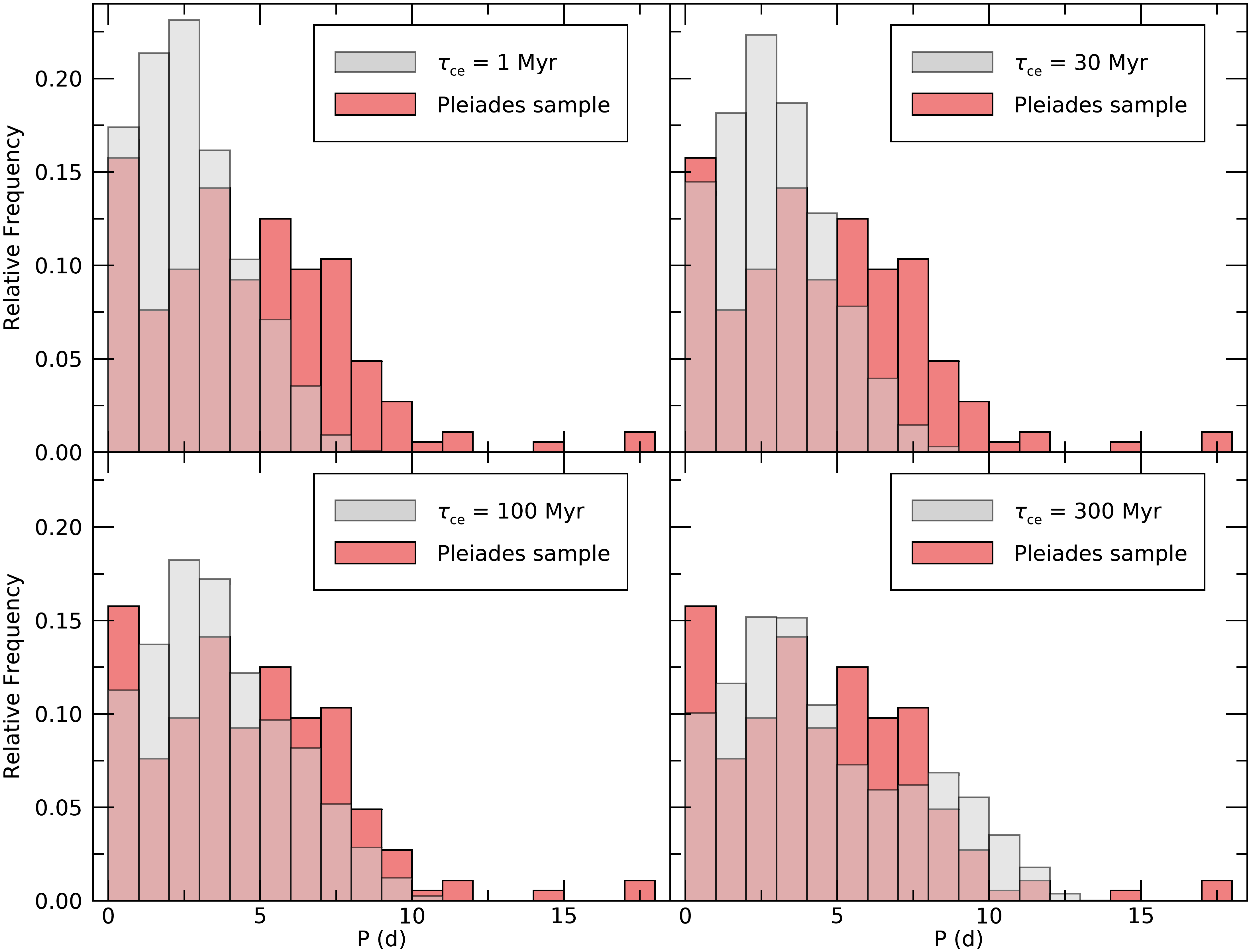
Figure 8: Simulated period distributions at 125 Myr obtained with $\tau_{\mathrm{ce}}$ equal to 1 Myr (top left panel), 30 Myr (top right panel), 100 Myr (bottom left panel) and 300 Myr (bottom right panel) superimposed to observational data of the Pleiades.

Table 4: K-S tests results comparing the simulated period distributions and the observational period distributions using different $\tau_{\mathrm{ce}}$ values.

Cluster	$\tau_{\mathrm{ce}}$ values (Myr)
	1	30	100	300	300, 300, 1
ONC	0.08	0.09	0.09	0.09	0.08
Cyg OB2	0.15	0.15	0.15	0.15	0.15
NGC 2362	0.11	0.11	0.11	0.11	0.11
U Sco	0.10	0.11	0.10	0.11	0.10
h Per	0.18	0.18	0.18	0.18 0.18
Pleiades	0.33	0.30	0.17	0.08	0.08
M37	0.33	0.09	0.15	0.097	0.10

2.2.3 Model M3

Examining Table 3, we note that model M1 is successful in explaining three out of four clusters younger than h Per but it cannot reproduce the older clusters taken for comparison in this work. We can wonder if the problem is related to our initial conditions, to the assumed disk locking mechanism, to the wind prescription or to the core-envelope angular momentum exchange. In order to rule out the first two uncertainties, we decided to run model M3 similarly to what was done by Coker et al. (2016). This model begins at 13 Myr and its initial period distribution is taken from the observational period distribution of h Per (Moraux et al., 2013) but otherwise it is similar to model M1, using the same wind prescription and the same core-envelope coupling timescale values.

In Fig. 9 we show the period distributions obtained with model M3 at 13 Myr, 125 Myr and 550 Myr compared to observational distributions of h Per, the Pleiades and M37.

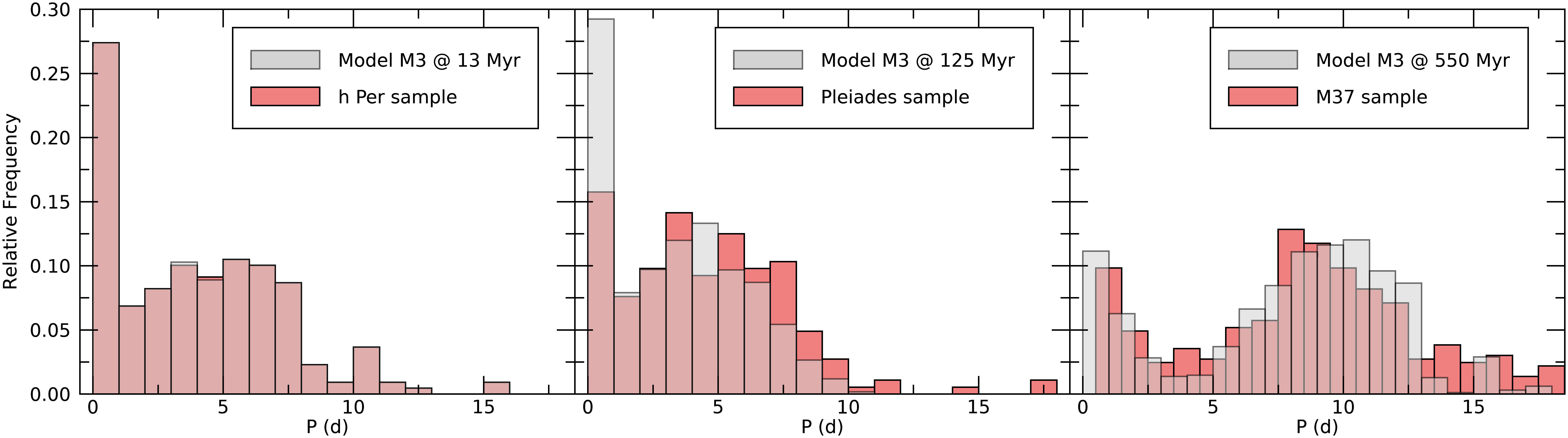
Figure 9: Simulated period distributions at 13 Myr, 125 Myr and 550 Myr obtained with model M3 superimposed to observational data of h Per, the Pleiades and M37.

At 13 Myr, the simulated and the observational distributions are almost perfectly superimposed. The maximal difference between the two cumulative distributions seen at the 5^th column at Table 3 is 0.01, much smaller than the critical one. Obviously, the two samples are derived from the same population as imposed by the initial conditions of this model. Even so, the Pleiades and M37 period distributions can not be reproduced by this model according to the values obtained from the KS tests. Visually however the simulated period distributions are much similar to the observed ones. The number of fast rotators increased a lot compared to what was obtained with the other models. At the age of the Pleiades, there is an excess of simulated stars with periods shorter than 1.0 day and between 2.0 and 5.0 days compared to the observational sample. On the other hand, there is a lack of simulated stars at longer periods. The simulated period distribution at the age of 550 Myr is very similar to the observed one.

We can conclude that the mechanisms (the wind mass loss prescription and/or the core-envelope coupling parameterization) and the parameters applied to this model produced a very good visual match of the distributions but not quantitatively enough to fully explain the observed period distributions. For MS clusters as old as M37 (550 Myr old) initial conditions seems to play a secondary role in the evolution of the angular momentum.

2.2.4 Other mass distributions

Young open clusters appear to have similar intrinsic mass functions (Bastian et al., 2010; Damian et al., 2021). However, the observed samples do not evenly sample the intrinsic IMF. As a result, the mass distribution of the samples we use here does not exactly follow the underlying IMF. In order to take this observational bias into account, we computed models similar to model M1 with a finer mass grid reproducing the mass distributions of the observed samples used in this work. Now the mass range goes from 0.5 to 1.1 M_⊙ in intervals of 0.1 M_⊙ values. The percentage value at each mass bin is shown in Table 5 and can be seen in Fig. 10.

Table 5: Kroupa’s IMF and mass distributions of the selected young clusters.

MF	0.5 M⊙	0.6 M⊙	0.7 M⊙	0.8 M⊙	0.9 M⊙	1.0 M⊙	Reference
	%
Kroupa	34	22	16	12	9	7	1
ONC	22	43	22	8	1	4	2, 3
Cyg OB2	51	28	13	6	1	1	4
h Per	17	14	12	18	18	20	5
Pleiades	28	23	14	13	12	10	6, 7

(1) Kroupa et al. (2013), (2) Cieza & Baliber (2007), (3) Davies et al. (2014), (4) Roquette et al. (2017), (5) Moraux et al. (2013), (6) Rebull et al. (2016), (7) Lodieu et al. (2019).

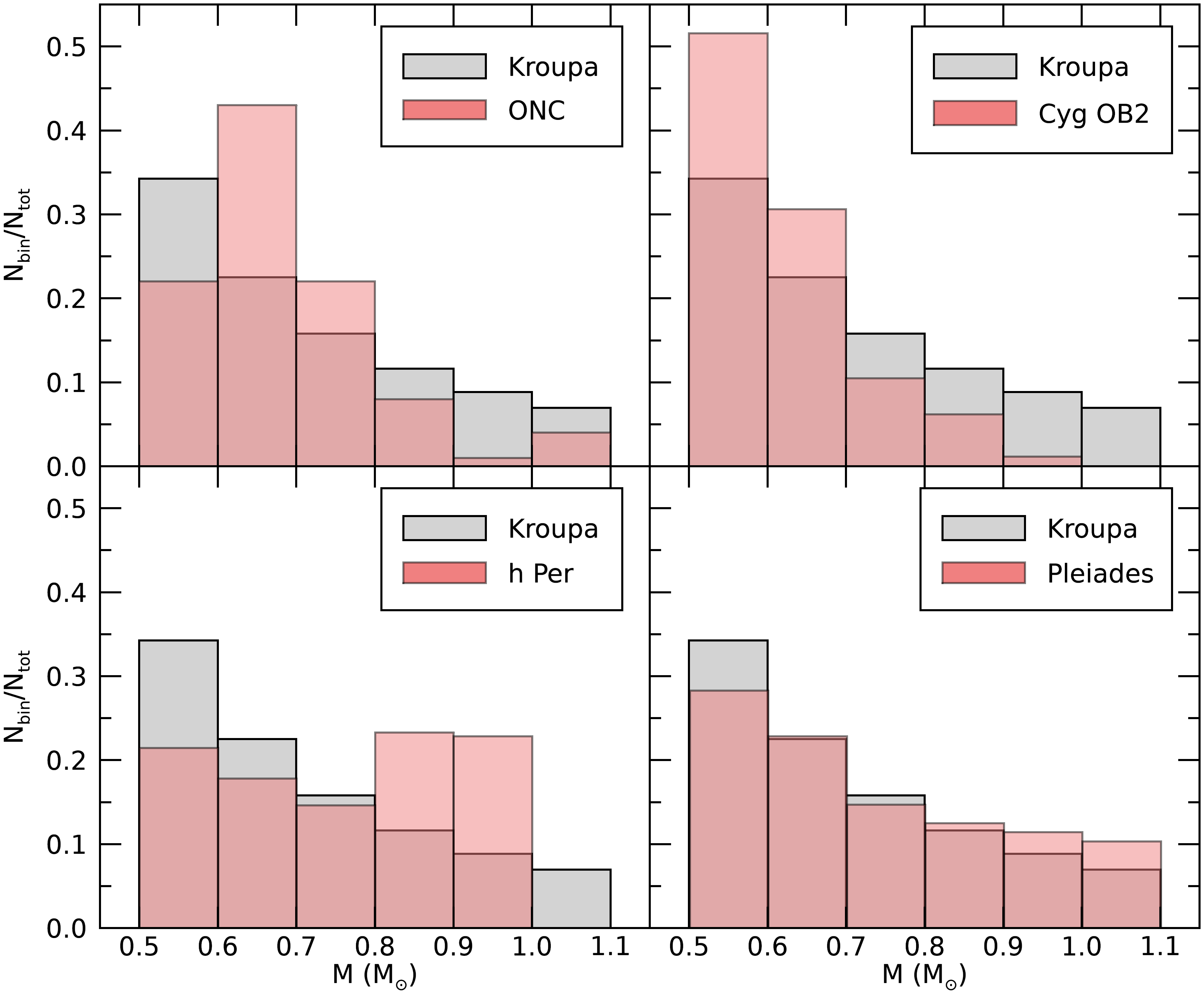
Figure 10: Comparison of mass distributions of the ONC, Cyg OB2, h Per and the Pleiades to Kroupa’s IMF.

The values at each mass bin for the Kroupa mass function were calculated using Kroupa et al. (2013) equations for the canonical IMF. The percentage of stars that appears in Table  5 was then calculated considering the total number of stars of the simulation. To calculate the other mass distributions we take the observational samples used in this work for which we have stellar mass values (a combined sample of Cieza & Baliber (2007) and Davies et al. (2014) for the ONC; Cyg OB2 from Roquette et al. (2017), h Per from Moraux et al. (2013) and a combined sample of Rebull et al. (2016) and Lodieu et al. (2019) for the Pleiades) and estimate the percentage of stars in the mass bins from the total number of stars in each sample. We then use these percentages to calculate the amount of objects in the mass bins for each one of the mass distributions shown in Table 6. Since the methods or models used by the different authors to assign mass to the observational samples are not the same the sample used here is not homogeneous.

When we analyze the angular velocity evolution for stars with different masses but with the same initial rotation periods and disk lifetimes at the age of 125 Myr, we note that their values do vary with mass (Figure 11). Considering stars in all the three initial rotating intervals (fast, median and slow rotators), the fastest rotating stars at 125 Myr are those of 0.5 M_⊙. However there is no monotonic relation between mass and rotation. Analyzing the fast rotators set, after the 0.5 M_⊙ star, follows stars of 0.6, 0.8, 0.7, 0.9 and 1.0 M_⊙ in order of decreasing angular velocity. In the group of median rotators, the sequence of decreasing angular velocity is again of stars of 0.5 and 0.6 M_⊙ and then stars of 1.0, 0.8 and 0.9 and 0.7 M_⊙. For the slow rotators, it is 0.5, 1.0, 0.9, 0.8 and 0.6 and 0.7 M_⊙. Clearly, 0.5 M_⊙ stars stay longer at the PMS phase, spinning up due to radius contraction. At 125 Myr, they still present a high spin rate.

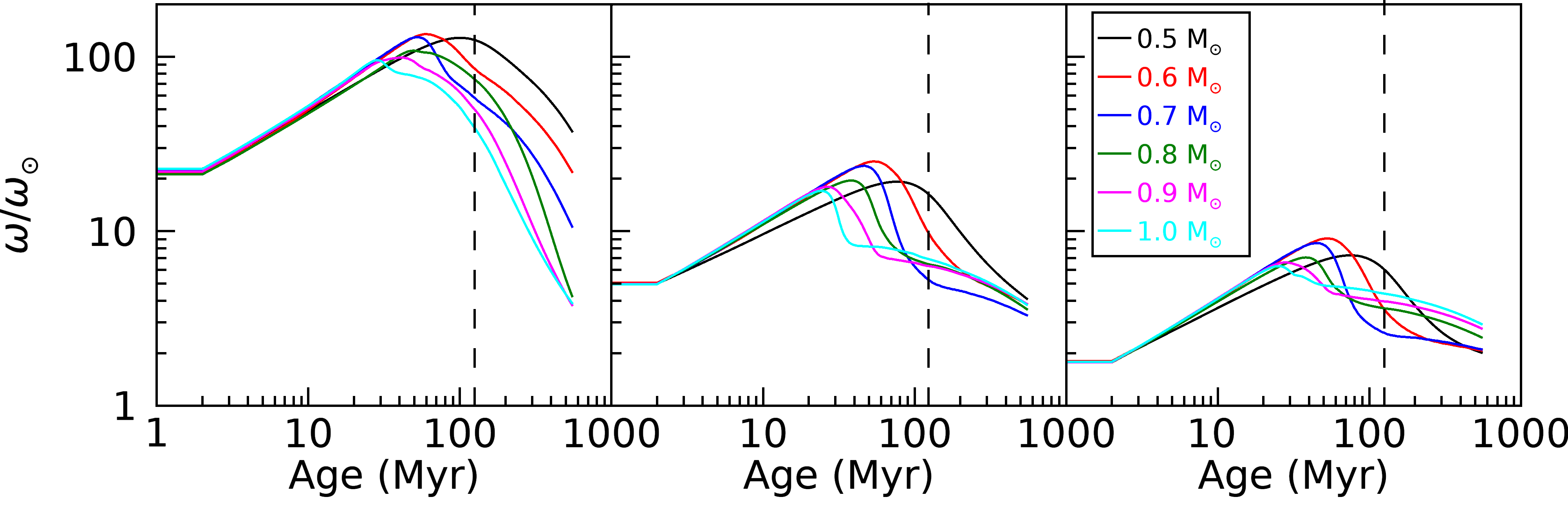
Figure 11: Angular velocity evolution as a function of age considering stars with masses between 0.5 and 1.0 M_⊙ and with a disk lifetime equal to 1 Myr. In the left panel, all stars are fast rotators (see text for a definition) and have approximately the same initial rotational period. In the middle and right panels we have, respectively, median and slow rotators. The vertical dashed line mark the age of 125 Myr.

Therefore, mass distributions (MD) that have a high fraction of low mass (0.5 and 0.6 M_⊙) stars will present a higher number of stars with rotational periods below 1.0 day (the first bin of the rotational period distributions - Figure 12) although stars at this mass range also produce the fastest rotators of the other rotational intervals (medium and slow). This is the case of the results obtained with the Cyg OB2 MD and the Kroupa IMF in model M1 (Figure 10 and the left panels of Figure 12). On the opposite side, the period distribution obtained with a model that uses the h Per MD that has a deficit of 0.5 M_⊙ star shows the lowest number of stars with periods shorter than 1.0 d. The results obtained using the Pleiades MD that is very similar to Kroupa IMF with 7 mass bins produces a different period distribution, however, due to the lower number of 0.5 M_⊙ stars and a slightly higher fraction of 0.8 - 1.1 M_⊙ stars. The objects that are initially classified as medium rotators, at 125 Myr show periods between $\sim$ 2 and 5 days and the initially slow rotators populate the longer period bins. The period distribution obtained with the ONC MD is not so visually different but produces statistically different values from that obtained with the Kroupa IMF (Table 6). The ONC MD has less 0.5 M_⊙ stars but an excess of 0.6 and 0.7 M_⊙ stars compared to the Kroupa IMF (Figure 10).

In Table 6 the K-S statistics of the models with different MD is shown. One thing to be noticed is that the K-S distances obtained using Kroupa’s IMF (2^nd column) are slightly different from model M1’s except for the Pleiades for which they are much different and smaller. Although none of the mass distributions are similar to Kroupa’s IMF, the critical distances obtained from K-S tests are alike among the pre main-sequence clusters (from ONC to h Per) and comparable to the values obtained from model M1. For the Pleiades they are much smaller and different for the various mass distributions. Now, statistically there is an agreement between the models at 125 Myr and the observed Pleiades period distribution (but not for the model that uses Cyg OB2 mass distribution). For M37, the K-S distance values are similar to those obtained with model M1 but they are more sensitive to the different mass distributions compared to the PMS clusters.

Table 6: K-S tests results comparing the simulated period distributions for all stars and the observational period distributions using different IMF.

MF	Kroupa∗	ONC	Cyg OB2	h Per	Pleiades
Cluster	DKS					$D_{\mathrm{crit}}$
ONC	0.08	0.08	0.08	0.08	0.08	0.128
Cyg OB2	0.15	0.14	0.15	0.17	0.16	0.084
NGC 2362	0.13	0.14	0.13	0.14	0.10	0.14
U Sco	0.095	0.097	0.095	0.10	0.10	0.11
h Per	0.17	0.17	0.18	0.16	0.17	0.092
Pleiades	0.097	0.07	0.16	0.10	0.08	0.096
M37	0.099	0.094	0.086	0.14	0.10	0.071

^∗ The difference between the K-S statistical for the model using Kroupa’s IMF and that seen in Table 3 is due to the difference on the models mass range.

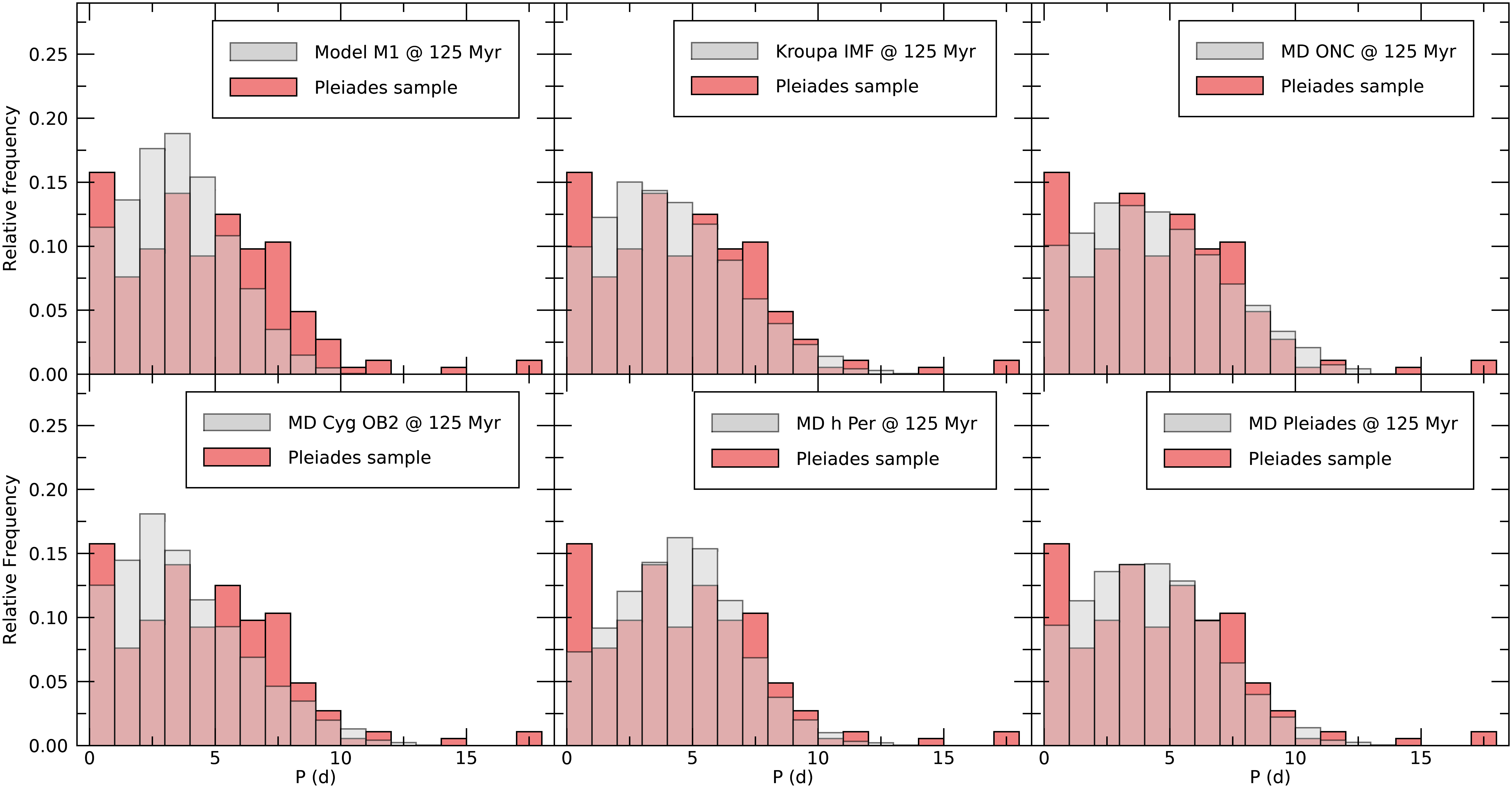
Figure 12: Rotational period distributions at 125 Myr obtained with model M1 and the mass distributions show in Table 5 and in Figure 10 all of them superimposed on Pleiades observational period distribution. Top panels from left to right: model M1 and models using Kroupa IMF with 7 mass bins and the ONC MD. Bottom panels, from left to right: models using Cyg OB2, h Per and Pleiades mass distributions.

In Figure 13, we show the cumulative distributions (CD) relative to the period distributions seen in Figure 12, with the point of maximal distance between the observational Pleiades period distribution and the models marked by a vertical dotted line. The conclusions stated previously appear more clearly after an inspection of Figure 13. We see that, despite the fact that in model M1 and in this section we present results that uses the same IMF of Kroupa, the absence of some of the mass bins makes the cumulative distributions different (1^st and 2^nd top panels of Figure 13). We also note that the CD obtained using model M1 and Cyg OB 2 MD are very similar, with the maximal difference between the observed and the model theoretical cumulative distributions occurring at the same period. However, in model M1 there is an excess of objects with periods longer than 3 days and this causes the saturation of CD earlier than in the Cyg OB2 CD. There is a deficit of objects with short rotational periods and an excess of longer period objects when we examine the CD obtained through the model with the h Per MD. Also, we can clearly see why the model with the ONC MD produces better statistical results than those using Kroupa IMF and Pleiades MD at 125 Myr since the simulated and the observational cumulative distributions fit very well.

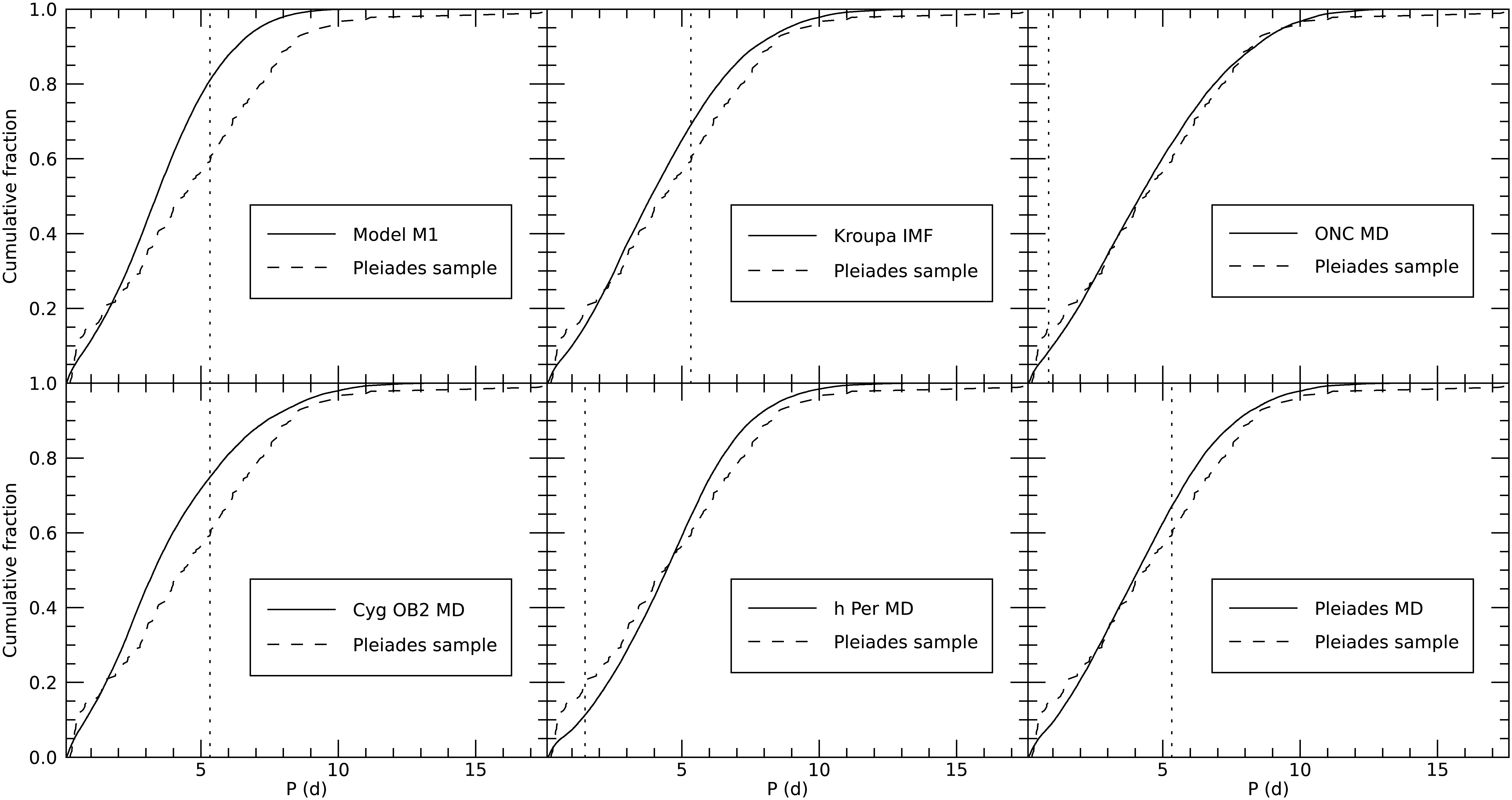
Figure 13: Cumulative period distributions at 125 Myr obtained with model M1 and the mass distributions show in Table 5 and in Figure 10 (solid lines) all of them superimposed on Pleiades observational cumulative period distribution (dashed lines). Top panels from left to right: model M1 and models using Kroupa IMF with 7 mass bins and the ONC MD. Bottom panels, from left to right: models using Cyg OB2, h Per and Pleiades mass distributions. Also shown is a vertical line marking the corresponding period where the maximal difference between of simulated and observational samples occurs (dotted lines).

3 Conclusions

In this work, we analyzed the rotational evolution of solar mass stars from 1 Myr to 550 Myr taking into account disk locking, core-envelope decoupling and angular momentum loss via a magnetized wind.

Our standard model, model M1, reproduces well the disk fraction as a function of age and the rotational period distributions of PMS clusters younger than 13 Myr old.

We test the role the core-envelope coupling timescale has in our simulations. At the pre-main sequence and ZAMS this parameter does not seem to influence greatly the period distributions. It is more important at the MS and it is necessary to have a weak coupling (high $\tau_{\mathrm{ce}}$ values) for slow and medium rotators in order to reproduce the observations.

We also run simulations assuming different values for the disk lifetimes and for the initial period distributions. While these models provide synthetic rotational period distributions resembling those of observed clusters, they do not fulfill the quantitative similarity criteria set by the K-S test. Running a finer grid model and replacing the Kroupa’s initial mass function by the empirical mass functions of the samples studied here did not produce any significant improvement compared to model M1 except for the Pleiades that now are reproduced by our model.

It seems that there are some intrinsic differences among the clusters related to their initial conditions. For example, enhanced disk dissipation in massive clusters, multiplicity fraction, planet formation in disks and the role magnetic fields play in the first stages of the stellar formation may change the initial rotation pattern of the population of different clusters. This could explain the different rotation patterns observed in the clusters of about the same age Cyg OB2 and NGC 2362 or U Sco and h Per. These aspects are interesting and will be analyzed in future works as well as the impact of the use of different stellar models that take into account accretion and rotation and the lithium-rotation connection problem.

We can conclude that in a global perspective the secular evolution of rotation described by the models presented here grasp the main trends of the spin evolution of low-mass stellar populations. However specific clusters may keep signatures of their initial conditions up to at least the ZAMS as it seems to be case for the pre-main sequence clusters analyzed in this work, from the ONC to h Per. Eventually, a physical description of the star-disk interaction process that prevents PMS stars from spinning-up during the disk locking phase remains to be provided.

Data Availability

The data underlying this article will be shared on reasonable request to the corresponding author.

References

- Allain (1998) Allain S., 1998, A&A, 333, 629
- Amard et al. (2019) Amard L., Palacios A., Charbonnel C., Gallet F., Georgy C., Lagarde N., Siess L., 2019, A&A, 631, A77
- Baraffe & Chabrier (2010) Baraffe I., Chabrier G., 2010, A&A, 521, A44
- Baraffe et al. (1998) Baraffe I., Chabrier G., Allard F., Hauschildt P. H., 1998, A&A, 337, 403
- Barnes (2010) Barnes S. A., 2010, ApJ, 722, 222
- Barnes & Kim (2010) Barnes S. A., Kim Y.-C., 2010, ApJ, 721, 675
- Bastian et al. (2010) Bastian N., Covey K. R., Meyer M. R., 2010, ARA&A, 48, 339
- Berlanas et al. (2018) Berlanas S. R., Herrero A., Comerón F., Simón-Díaz S., Cerviño M., Pasquali A., 2018, A&A, 620, A56
- Biazzo et al. (2011) Biazzo K., Randich S., Palla F., 2011, A&A, 525, A35
- Bouvier et al. (2014) Bouvier J., Matt S. P., Mohanty S., Scholz A., Stassun K. G., Zanni C., 2014, Protostars and Planets VI, pp 433–450
- Casamiquela et al. (2017) Casamiquela L., et al., 2017, MNRAS, 470, 4363
- Chaboyer et al. (1995) Chaboyer B., Demarque P., Pinsonneault M. H., 1995, ApJ, 441, 876
- Cieza & Baliber (2007) Cieza L., Baliber N., 2007, ApJ, 671, 605
- Coker et al. (2016) Coker C. T., Pinsonneault M., Terndrup D. M., 2016, ApJ, 833, 122
- Concha-Ramírez et al. (2021) Concha-Ramírez F., Wilhelm M. J. C., Portegies Zwart S., van Terwisga S. E., Hacar A., 2021, MNRAS, 501, 1782
- Covey et al. (2016) Covey K. R., et al., 2016, ApJ, 822, 81
- Cranmer & Saar (2011) Cranmer S. R., Saar S. H., 2011, ApJ, 741, 54
- D’Orazi et al. (2009) D’Orazi V., Randich S., Flaccomio E., Palla F., Sacco G. G., Pallavicini R., 2009, A&A, 501, 973
- Damian et al. (2021) Damian B., Jose J., Samal M. R., Moraux E., Das S. R., Patra S., 2021, arXiv e-prints, p. arXiv:2101.08804
- Davies et al. (2014) Davies C. L., Gregory S. G., Greaves J. S., 2014, MNRAS, 444, 1157
- Demarque et al. (2008) Demarque P., Guenther D. B., Li L. H., Mazumdar A., Straka C. W., 2008, Ap&SS, 316, 31
- Dufton et al. (1990) Dufton P. L., Brown P. J. F., Fitzsimmons A., Lennon D. J., 1990, A&A, 232, 431
- Edwards et al. (1993) Edwards S., et al., 1993, AJ, 106, 372
- Ferreira et al. (2000) Ferreira J., Pelletier G., Appl S., 2000, MNRAS, 312, 387
- Gallet & Bouvier (2013) Gallet F., Bouvier J., 2013, A&A, 556, A36
- Gallet & Bouvier (2015) Gallet F., Bouvier J., 2015, A&A, 577, A98
- Gallet et al. (2019) Gallet F., Zanni C., Amard L., 2019, A&A, 632, A6
- Ghosh & Lamb (1979) Ghosh P., Lamb F. K., 1979, ApJ, 234, 296
- Gondoin (2017) Gondoin P., 2017, A&A, 599, A122
- Guarcello et al. (2013) Guarcello M. G., et al., 2013, ApJ, 773, 135
- Guarcello et al. (2021) Guarcello M. G., et al., 2021, A&A, 650, A157
- Hartman et al. (2008) Hartman J. D., et al., 2008, ApJ, 675, 1233
- Hartman et al. (2009) Hartman J. D., et al., 2009, ApJ, 691, 342
- Hartman et al. (2010) Hartman J. D., Bakos G. Á., Kovács G., Noyes R. W., 2010, MNRAS, 408, 475
- Hartmann et al. (1998) Hartmann L., Calvet N., Gullbring E., D’Alessio P., 1998, ApJ, 495, 385
- Herczeg & Hillenbrand (2015) Herczeg G. J., Hillenbrand L. A., 2015, ApJ, 808, 23
- Hernández et al. (2007) Hernández J., et al., 2007, ApJ, 662, 1067
- Hernández et al. (2008) Hernández J., Hartmann L., Calvet N., Jeffries R. D., Gutermuth R., Muzerolle J., Stauffer J., 2008, ApJ, 686, 1195
- Ireland et al. (2021) Ireland L. G., Zanni C., Matt S. P., Pantolmos G., 2021, ApJ, 906, 4
- Irwin et al. (2007) Irwin J., Hodgkin S., Aigrain S., Hebb L., Bouvier J., Clarke C., Moraux E., Bramich D. M., 2007, MNRAS, 377, 741
- Irwin et al. (2008) Irwin J., Hodgkin S., Aigrain S., Bouvier J., Hebb L., Irwin M., Moraux E., 2008, MNRAS, 384, 675
- Kawaler (1988) Kawaler S. D., 1988, ApJ, 333, 236
- Koenigl (1991) Koenigl A., 1991, ApJ, 370, L39
- Kroupa et al. (2013) Kroupa P., Weidner C., Pflamm-Altenburg J., Thies I., Dabringhausen J., Marks M., Maschberger T., 2013, The Stellar and Sub-Stellar Initial Mass Function of Simple and Composite Populations. p. 115, doi:10.1007/978-94-007-5612-0_4
- Landin et al. (2016) Landin N. R., Mendes L. T. S., Vaz L. P. R., Alencar S. H. P., 2016, A&A, 586, A96
- Lanzafame & Spada (2015) Lanzafame A. C., Spada F., 2015, A&A, 584, A30
- Littlefair et al. (2010) Littlefair S. P., Naylor T., Mayne N. J., Saunders E. S., Jeffries R. D., 2010, MNRAS, 403, 545
- Lodieu et al. (2019) Lodieu N., Pérez-Garrido A., Smart R. L., Silvotti R., 2019, A&A, 628, A66
- MacGregor & Brenner (1991) MacGregor K. B., Brenner M., 1991, ApJ, 376, 204
- Matt & Pudritz (2005) Matt S., Pudritz R. E., 2005, ApJ, 632, L135
- Matt et al. (2012) Matt S. P., MacGregor K. B., Pinsonneault M. H., Greene T. P., 2012, ApJ, 754, L26
- Matt et al. (2015) Matt S. P., Brun A. S., Baraffe I., Bouvier J., Chabrier G., 2015, ApJ, 799, L23
- Mayne & Naylor (2008) Mayne N. J., Naylor T., 2008, MNRAS, 386, 261
- Moraux et al. (2013) Moraux E., et al., 2013, A&A, 560, A13
- Netopil et al. (2016) Netopil M., Paunzen E., Heiter U., Soubiran C., 2016, A&A, 585, A150
- Padgett (1996) Padgett D. L., 1996, ApJ, 471, 847
- Pecaut et al. (2012) Pecaut M. J., Mamajek E. E., Bubar E. J., 2012, ApJ, 746, 154
- Rebull et al. (2004) Rebull L. M., Wolff S. C., Strom S. E., 2004, AJ, 127, 1029
- Rebull et al. (2006) Rebull L. M., Stauffer J. R., Megeath S. T., Hora J. L., Hartmann L., 2006, ApJ, 646, 297
- Rebull et al. (2016) Rebull L. M., et al., 2016, AJ, 152, 113
- Rebull et al. (2017) Rebull L. M., Stauffer J. R., Hillenbrand L. A., Cody A. M., Bouvier J., Soderblom D. R., Pinsonneault M., Hebb L., 2017, ApJ, 839, 92
- Rebull et al. (2018) Rebull L. M., Stauffer J. R., Cody A. M., Hillenbrand L. A., David T. J., Pinsonneault M., 2018, AJ, 155, 196
- Rebull et al. (2020) Rebull L. M., Stauffer J. R., Cody A. M., Hillenbrand L. A., Bouvier J., Roggero N., David T. J., 2020, AJ, 159, 273
- Ribas et al. (2014) Ribas Á., Merín B., Bouy H., Maud L. T., 2014, A&A, 561, A54
- Romanova et al. (2009) Romanova M. M., Ustyugova G. V., Koldoba A. V., Lovelace R. V. E., 2009, MNRAS, 399, 1802
- Roquette et al. (2017) Roquette J., Bouvier J., Alencar S. H. P., Vaz L. P. R., Guarcello M. G., 2017, A&A, 603, A106
- Roquette et al. (2021) Roquette J., Matt S. P., Winter A. J., Amard L., Stasevic S., 2021, MNRAS, 508, 3710
- Shu et al. (1994) Shu F., Najita J., Ostriker E., Wilkin F., Ruden S., Lizano S., 1994, ApJ, 429, 781
- Slesnick et al. (2008) Slesnick C. L., Hillenbrand L. A., Carpenter J. M., 2008, ApJ, 688, 377
- Smartt & Rolleston (1997) Smartt S. J., Rolleston W. R. J., 1997, ApJ, 481, L47
- Soderblom et al. (2014) Soderblom D. R., Hillenbrand L. A., Jeffries R. D., Mamajek E. E., Naylor T., 2014, in Beuther H., Klessen R. S., Dullemond C. P., Henning T., eds, Protostars and Planets VI. p. 219 (arXiv:1311.7024), doi:10.2458/azu_uapress_9780816531240-ch010
- Somers & Pinsonneault (2015) Somers G., Pinsonneault M. H., 2015, MNRAS, 449, 4131
- Southworth et al. (2004) Southworth J., Maxted P. F. L., Smalley B., 2004, MNRAS, 349, 547
- Spada & Lanzafame (2020) Spada F., Lanzafame A. C., 2020, A&A, 636, A76
- Spada et al. (2011) Spada F., Lanzafame A. C., Lanza A. F., Messina S., Collier Cameron A., 2011, MNRAS, 416, 447
- Stauffer et al. (1998) Stauffer J. R., Schultz G., Kirkpatrick J. D., 1998, ApJ, 499, L199
- Takeda et al. (2017) Takeda Y., Hashimoto O., Honda S., 2017, PASJ, 69, 1
- Tamajo et al. (2011) Tamajo E., Pavlovski K., Southworth J., 2011, A&A, 526, A76