Joint Synthesis of Safety Certificate and Safe Control Policy using Constrained Reinforcement Learning

Abstract

Safety is the major consideration in controlling complex dynamical systems using reinforcement learning (RL), where the safety certificates can provide provable safety guarantees. A valid safety certificate is an energy function indicating that safe states are with low energy, and there exists a corresponding safe control policy that allows the energy function to always dissipate. The safety certificates and the safe control policies are closely related to each other and both challenging to synthesize. Therefore, existing learning-based studies treat either of them as prior knowledge to learn the other, limiting their applicability to general systems with unknown dynamics. This paper proposes a novel approach that simultaneously synthesizes the energy-function-based safety certificates and learns the safe control policies with constrained reinforcement learning (CRL). We do not rely on prior knowledge about either a prior control law or a perfect safety certificate. In particular, we formulate a loss function to optimize the safety certificate parameters by minimizing the occurrence of energy increases. By adding this optimization procedure as an outer loop to the Lagrangian-based CRL, we jointly update the policy and safety certificate parameters, and prove that they will converge to their respective local optima, the optimal safe policies and valid safety certificates. Finally, we evaluate our algorithms on multiple safety-critical benchmark environments. The results show that the proposed algorithm learns solidly safe policies with no constraint violation. The validity or feasibility of synthesized safety certificates is also verified numerically.

1 Introduction

Safety is critical when applying state-of-the-art artificial intelligence studies to real-world applications, like autonomous driving (Sallab et al., 2017; Chen et al., 2021), robotic control (Richter et al., 2019; Ray et al., 2019). Safe control is one of the most common tasks among these real-world applications, requiring that the hard safety constraints must be obeyed persistently. However, learning a safe control policy is hard for the naive trial-and-error mechanism of RL since it penalizes the dangerous actions after experiencing them.

Meanwhile, in the control theory, there exist studies about energy-function-based provable safety guarantee of dynamic systems called the safety certificate, or safety index (Wieland and Allgöwer, 2007; Ames et al., 2014; Liu and Tomizuka, 2014). These methods first synthesize energy functions such that the safe states have low energy, then design control laws satisfying the safe action constraints to make the systems dissipate energy (Wei and Liu, 2019). If there exists a feasible policy for all states in a safe set to satisfy the safe action constraints dissipating the energy, the system will never leave the safe set (i.e., forward invariance). Despite its soundness, the safety index synthesis (SIS) by hand is extremely hard for complex systems, which stimulates a rapidly growing interest in learning-based SIS (Chang et al., 2020; Saveriano and Lee, 2019; Srinivasan et al., 2020; Ma et al., 2021a; Qin et al., 2021). Nevertheless, These studies usually require known dynamical models (white-box, black-box or learning-calibrated) to design control laws. Furthermore, obtaining the policy satisfying safe action constraints is also challenging. Adding safety shields or layers to obtain supervised RL policies is a common approach (Wang et al., 2017; Agrawal and Sreenath, 2017; Cheng et al., 2019; Taylor et al., 2020), but these studies usually assume to know the valid safety certificates.

In general safe control tasks with unknown dynamics, one usually has access to neither the control laws nor perfect safety certificates, which makes the previous two kinds of studies fall into a paradox—they rely on each other as the prior knowledge. Therefore, this paper proposes a novel algorithm without prior knowledge about model-based control laws or valid safety certificates. We define a loss function for SIS by minimizing the occurrence of energy increases. Then we formulate a CRL problem (rather than the commonly used shield methods) to unify the loss functions of SIS and CRL. By adding SIS as an outer loop to the Lagrangian-based solution to CRL, we jointly update the policies and safety certificates, and prove that they will converge to their respective local optima, the optimal safe policies and the valid safety certificates.

Contributions. Our main contributions are: 1. We propose an algorithm of joint CRL and SIS that learns the safe policies and synthesizes the safety certificates simultaneously. This is the first algorithm requiring no prior knowledge of control laws or valid safety certificates. 2. We unify the loss function formulations of SIS and CRL. We therefore can form the multi-timescale adversarial RL training and prove its convergence. 3. We evaluate the proposed algorithm on multiple safety-critical benchmark environments Results demonstrate that we can simultaneously synthesize valid safety certificates and learn safe policies with zero constraint violation.

1.1 Related works

Representative energy-function-based safety certificates include barrier certificates (Prajna et al., 2007), control barrier functions (CBF) (Wieland and Allgöwer, 2007), safety set algorithm (SSA) (Liu and Tomizuka, 2014) and sliding mode methods (Gracia et al., 2013). Recent learning-based studies can be mainly divided into learning-based SIS and learning safe control policies supervised by certificates. Chang et al. (2020); Luo and Ma (2021) use explicit models to rollout or project actions to satisfy safe action constraints. Jin et al. (2020); Qin et al. (2021) guide certificate learning with LQR controllers, Zhao et al. (2021) requires a black-box model to query online, and Saveriano and Lee (2019); Srinivasan et al. (2020) use labeled data to fit certificates with supervised learning. The latter one, learning safe policy with supervisory usually assumed a valid safety certificate (Wang et al., 2017; Cheng et al., 2019; Taylor et al., 2020). It’s a natural thought that one could learn the dynamic models to handle these issues (like Cheng et al., 2019; Luo and Ma, 2021), but learning models is much more complex than only learning policies, especially in RL tasks.

2 Problem Formulations

We consider the safety specification that the system state $s$ should be constrained in a connected and closed set $\mathcal{S}_{s}$ which is called the safe set. $\mathcal{S}_{s}$ should be a zero-sublevel set of a safety index function $\phi_{0}(\cdot)$ denoted by $\mathcal{S}_{s}=\{s|\phi_{0}(s)\leq 0\}$. We study the Markov decision process (MDP) with deterministic dynamics (a reasonable assumption when dealing with safe control problems), defined by the tuple $(\mathcal{S},\mathcal{A},\mathcal{F},r,c,\gamma,\phi)$, where $\mathcal{S},\mathcal{A}$ is the state and action space, $\mathcal{F}:\mathcal{S}\times\mathcal{A}\to\mathcal{S}$ is the unknown system dynamics, $r,c:\mathcal{S}\times\mathcal{A}\times\mathcal{S}\rightarrow\mathbb{R}$ is the reward and cost function, $\gamma$ is the discounted factor, and $\phi:\mathcal{S}\to\mathbb{R}$ is the energy-function-based safety certificate, or called the safety index. A safe control law with respect to safety index $\phi$ should keep the system energy low, ($\phi\leq 0$) and dissipate the energy when the system is at high energy ($\phi>0$). We use $s^{\prime}$ to represent the next state for simplicity. Then we can get the safe action constraint:

Definition 2.1 (Safe action constraint).

For a given safety index $\phi$, the safe action constraint is

$$\phi(s^{\prime})<\max\{\phi(s)-\eta_{D},0\}$$ (1)

where $\eta_{D}$ is a slack variable controlling the descent rate of safety index.

Definition 2.2 (Valid safety certificate).

If there always exists an action $a\in\mathcal{A}$ satisfying eq:cstr0 at $s$, or the safe action set $\mathcal{U}_{s}(s)=\{a|\phi(s^{\prime})<\max\{\phi(s)-\eta_{D},0\}\}$ is always nonempty, we say the safety index $\phi$ is a valid, or feasible safety certificate.

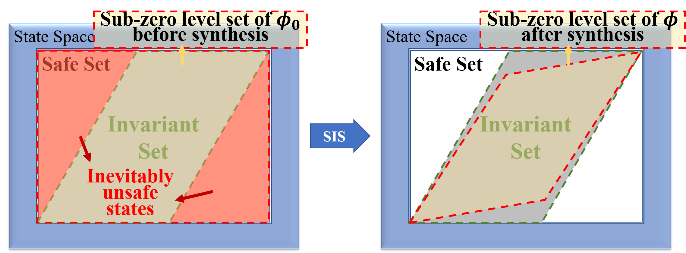
Figure 1: Safety index synthesis (SIS). Inevitably unsafe states should be excluded during the SIS.

A straightforward approach is to use the $\phi_{0}$ as the safety certificate. However, these safe action constraints are possibly not satisfied with all the states in $\mathcal{S}_{s}$ as shown in fig:intro. This problem is common in real-world tasks with actuator saturation and high relative-degree from safety specifications to control inputs (i.e., $\|\frac{\partial\phi_{0}}{\partial u}\|=0$). For example, if $\phi_{0}$ measures the distance between two autonomous vehicles, the collision may be inevitable because the relative speed is too high and brake force is limited. In this case, $\mathcal{S}_{s}$ includes inevitably unsafe states. We need to assign high energy values to these inevitably-unsafe states, for example, by linearly combining the $\phi_{0}$ and its high-order derivatives (Liu and Tomizuka, 2014). The valid safety certificate will guarantee safety by ensuring the forward invariance of a subset of $\mathcal{S}_{s}$.

Lemma 2.3 (Forward invariance (Liu and Tomizuka, 2014)).

Define the zero-sublevel set of a valid safety index $\phi$ as $\mathcal{S}_{s}^{\phi}=\{s|\phi(s)\leq 0\}$. If $\phi$ is a valid safety certificate, then there exist policies to guarantee the forward invariance of $\mathcal{S}_{s}^{\phi}\cap\mathcal{S}_{s}$.

We therefore can formulate the CRL problem by adding the safe action constraints to RL optimization objective:

$$\max_{\pi}\ \mathbb{E}_{\tau\sim\pi}\Big{\{}\sum\nolimits_{t=0}^{\infty}\gamma^{t}r_{t}\Big{\}}=\mathbb{E}_{s}\big{\{}v^{\pi}(s)\big{\}}\quad\text{s.t.}\ \phi(s^{\prime})-\max\{\phi(s)-\eta_{D},0\}<0,\forall s\in\mathcal{D}$$ (2)

where $v^{\pi}(s)$ is the state-value function of $s$, $\mathcal{D}=\{s|f(s)>0\}$ is the set of all possible states ($f$ is the state distribution density).

Remark 2.4.

eq:statewiseop has state-dependent constraints; it can not be solved by previous model-free CRL since their constraint objectives are defined on the expectation over $\mathcal{D}$ (Uchibe and Doya, 2007; Achiam et al., 2017; Chow et al., 2017; Tessler et al., 2018; Ray et al., 2019; Stooke et al., 2020).

We solve eq:statewiseop based on our previous framework to solve state-dependent safety constraints in (Ma et al., 2021b) using the Lagrange multiplier networks $\lambda(s)$ in a Lagrangian-based approach. The Lagrange function is (Ma et al., 2021b)

$$\mathcal{L}^{\prime}(\pi,\lambda)=\mathbb{E}_{s}\big{\{}-v^{\pi}(s)+\lambda(s)\big{(}\phi(s^{\prime})-\max\{\phi(s)-\eta_{D},0\}\big{)}\big{\}}$$ (3)

We can solve eq:statewiseop by locating the saddle point of $\mathcal{L}^{\prime}(\pi,\lambda)$, $\max_{\lambda}\min_{\pi}\mathcal{L}^{\prime}(\pi,\lambda)$.

3 Joint Synthesis of Safety Certificate and Safe Control Policy

The key idea of this section is to unify the loss functions of CRL and SIS; we provide theoretical analyses of their equivalence.

3.1 Loss Function for Safety Index Synthesis

We construct the loss for optimizing a parameterized safety index by a measurement of the violation of constraint eq:cstr0

$$J(\phi)=\left.\mathbb{E}_{s}\Big{\{}\left[\phi(s^{\prime})-\max\{\phi(s)-\eta_{D},0\}\right]^{+}\Big{\}}\right|_{\pi=\pi^{*}}$$ (4)

where $[\cdot]^{+}$ means projecting the values to the positive half-space $[0,+\infty)$, $\pi^{*}$ is the optimal safe policy (also a feasible policy when $\phi$ is a valid safety index) of eq:statewiseop, and $\cdot|_{\pi=\pi^{*}}$ represents the agent takes $\pi^{*}(s)$ to reach $s^{\prime}$. Ideally, if $\phi$ is a valid safety index, there always exists control to satisfy eq:cstr0, and $J(\phi)=0$. For those imperfect $\phi$, the inequality constraint in eq:statewiseop may not hold for all states in $\mathcal{D}$, so we can optimize the loss to get better $\phi$.

The joint synthesis algorithm is tricky since we need to handle two different optimization problems, eq:SL2 and eq:philoss1. Recent similar studies integrate two optimizations by weighted sum (Qin et al., 2021) or alternative update (Luo and Ma, 2021), but their methods are more like intuitive approaches and lack a solid theoretical basis.

3.2 Unified Loss Function for Joint Synthesis

Lemma 3.1 (Statewise complementary slackness condition (Ma et al., 2021b)).

For the problem eq:statewiseop, if the safe action set is not empty at state $s$, the optimal multiplier and optimal policy $\lambda^{*},\pi^{*}$ satisfies

$$\lambda^{*}(s)\{\phi(s^{\prime})-\max\{\phi(s)-\eta_{D},0\}|_{\pi*}\}=0$$ (5)

If the safe action set is empty at state $s$, then $\lambda^{*}(s)\to\infty$.

The lemma comes from the Karush-Kuhn-Tucker (KKT) necessary conditions for the problem eq:statewiseop.

Consider the Lagrange function eq:SL2 with the additional variable $\phi$ to optimize,

$$\mathcal{L}^{\prime}(\pi,\lambda,\phi)=\mathbb{E}_{s}\left\{-v^{\pi}(s)+\lambda(s)\big{(}\phi(s^{\prime})-\max\{\phi(s)-\eta_{D},0\}\big{)}\right\}$$ (6)

we have the following lemma for the relationship between the loss function of policy and certificate synthesis

Lemma 3.2.

If $\lambda$ is clipped into a compact set $[0,\lambda_{\max}]$, where $\lambda_{\max}>\max_{s\in\{s|\mathcal{U}_{s}(s)\neq\emptyset\}}\lambda^{*}(s)$. Then

$$\mathcal{L}^{\prime}(\pi^{*},\lambda^{*},\phi)=\lambda_{\max}J(\phi)+\Delta$$ (7)

where $\Delta$ is a constant irrelevant with $\phi$.

Proof 3.3.

See sec:proofpropto.

Theorem 3.4 (Unified loss for joint synthesis).

The optimal safety certificate parameters with optimal policy-multiplier tuple in eq:lagwithphi is also the optimal safety certificate parameters under loss in eq:philoss1

$$\arg\min J(\phi)=\arg\min\mathcal{L}^{\prime}(\pi^{*},\lambda^{*},\phi)$$ (8)

Proof 3.5.

See the envelope theorem on parameterized constraints in Milgrom and Segal (2002); Rockafellar (2015).

Finally, we unify the loss function of updating three elements: policy $\pi$, multiplier $\lambda$, and safety index function $\phi$. The optimization problem is formulated by a multi-timescale adversarial training:

$$\min_{\phi}\max_{\lambda}\min_{\pi}\mathcal{L}^{\prime}(\pi,\lambda,\phi)$$ (9)

4 Practical Algorithm using Constrained Reinforcement Learning

In this section, we explain the practical algorithm and convergence analysis.

4.1 Algorithm Details

The Lagrangian-based solution to CRL with statewise safety constraint is compatible with any existing unconstrained RL baselines, and we select the off-policy maximum entropy RL framework like soft actor-critic (SAC, Haarnoja et al., 2018a). According to eq:SL2, we need to add two neural networks to learn a state-action value function for safety index model $Q_{\phi}(s,a)$ (to approximate $\phi(s^{\prime})-\max\{\phi(s)-\eta_{D},0\}$) and the multipliers $\lambda(s)$. Because the soft policy evaluation, or the soft Q-learning part, is the same as Haarnoja et al. (2018a), we only demonstrate the soft policy iteration part of the algorithm in Algorithm 1. We name the proposed algorithm as FAC-SIS. We denote the parameters of the policy network, multiplier network, safety index as $\theta,\xi,\zeta$, respectively. We use $G_{\#},\ \#\in\{\theta,\xi,\zeta\}$ to denote the gradients to update policy, multiplier and certificate. Detailed computations of the gradients can be found in Appendix B.1. In addition, we assign multiple delayed updates (similar to Fujimoto et al., 2018), $m_{\pi}<m_{\lambda}<m_{\phi}$, to stabilize the adversarial optimizations.

Remark 4.1.

A general parameterization rule of safety index is to linearly combine $\phi_{0}$ and its high-order derivatives (Liu and Tomizuka, 2014), $\phi=\phi_{0}+k_{1}\dot{\phi_{0}}+\dots+k_{n}\phi_{0}^{(n)}$; the parameters $\xi$ is $[k_{1},k_{2},\dots,k_{n}]$. How many high-order derivatives are needed depends on the system relative-degree. For example, the relative-degree of position constraints with force inputs is $2$. This information should be included in observations of MDP. Otherwise, the observation can not fully describe how dangerous the agent is with respect to the safety constraint.

Algorithm 1 Soft Policy Improvement in FAC-SIS

0:  Buffer $\mathcal{D}$ with sampled data, policy parameters $\theta$, multiplier parameters $\xi$, safety index parameters $\zeta$.

1:  if gradient steps mod $m_{\pi}$ $=0$ then $\theta\leftarrow\theta-\overline{\beta_{\pi}}G_{\theta}$

2:  if gradient steps mod $m_{\lambda}$ $=0$ then $\xi\leftarrow\xi+\overline{\beta_{\lambda}}G_{\xi}$

3:  if gradient steps mod $m_{\phi}$ $=0$ then $\zeta\leftarrow\zeta-\overline{\beta_{\zeta}}G_{\zeta}$

3:  $w_{1}$, $w_{2}$, $\theta$, $\xi$.

4.2 Convergence Analysis

The convergence proof of a three timescale adversarial training of eq:minmaxmin mainly follows the multi-timescale convergence according to Theorem 2 in Chapter 6 in Borkar (2009) about multiple timescale convergence of multi-variable optimization. Some studies also adopted this procedure to explain the convergence of RL algorithms from the perspective of stochastic optimization (Bhatnagar et al., 2009; Bhatnagar and Lakshmanan, 2012), especially those with Lagrangian-based methods (Chow et al., 2017). We incorporate the recent study on clipped stochastic gradient descent to further improve the generalization of this convergence proof (Zhang et al., 2019). We first give some assumptions:

Assumption 1 (learning rates)

The learning rate schedules, $\{\beta_{\theta}(k),\beta_{\xi}(k),\beta_{\zeta}(k)\}$, satisfy

$$\notag\gathered{\small\sum\nolimits_{k}\beta_{\theta}(k)=\sum\nolimits_{k}\beta_{\xi}(k)=\sum\nolimits_{k}\beta_{\zeta}(k)=\infty.}\\ {\small\sum\nolimits_{k}\beta_{\theta}(k)^{2},\quad\sum\nolimits_{k}\beta_{\xi}(k)^{2},\quad\sum\nolimits_{k}\beta_{\zeta}(k)^{2}<\infty,\quad\beta_{\xi}(k)=o\left(\beta_{\theta}(k)\right),\ \beta_{\zeta}(k)=o\left(\beta_{\xi}(k)\right).}$$ (10)

This assumption also implies that the policy converges in the fastest timescale, then the multipliers, and finally the safety index parameters.

Proposition 4.2 (Clipped gradient descent).

The actual learning rate used in Algorithm 1 is

$$\overline{\beta_{\#}}:=\min\left\{\beta_{\#},{\beta_{\#}}/{\|G_{\#}\|}\right\}$$ (11)

where $\#\in\{w_{1},w_{2},\theta,\xi,\zeta\}$ is the parameters, and $G_{\#}$ is the corresponding gradients.

Assumption 2

The state and action are sampled from compact sets, and all neural networks are $L_{0}-L_{1}$ smooth.

As we are to finish a safe control problem that the agent should be confined in safe sets, and the actuator has physical limits, the bounded assumption is reasonable. We use multi-layer perceptron with continuous differentiable activation functions in practical implementations (details can be found in Appendix D).

Theorem 4.3.

Under all the aforementioned assumptions, the sequence of policy, multiplier, and safety index parameters tuple $(\theta_{k},\xi_{k},\zeta_{k})$ converge almost surely to a locally optimal safety index parameters and its corresponding locally optimal policy and multiplier $(\theta^{*},\xi^{*},\zeta^{*})$ as $k$ goes to infinity.

Proof 4.4.

See Appendix B.2.

5 Experiments

In our experiments, we focus on the following questions:

1. How does the proposed algorithm compare with other constraint RL algorithms? Can it achieve a safe policy with zero constraint violation?

2. How does the learning-based safety index synthesis outperform the handcrafted safety index or the original safety index in the safety performance?

3. Does the synthesized safety index allow safe control in all states the agent experienced?

To demonstrate the effectiveness of the proposed online synthesis rules, we select the safe reinforcement learning benchmark environments Safety Gym (Ray et al., 2019) with different tasks and obstacles. We name a specific environment by {Obstacle type}-{Obstacle size}-{Task}. We select six environments with different tasks and constraint objectives, where four of them are demonstrated in Figure 2, and others are provided in sec:addexpgym.

Remark 5.1.

Some previous studies use controllers specially designed for goal-reaching tasks (Jin et al., 2020; Qin et al., 2021), while our algorithm can handle arbitrary complex tasks like the Push tasks.

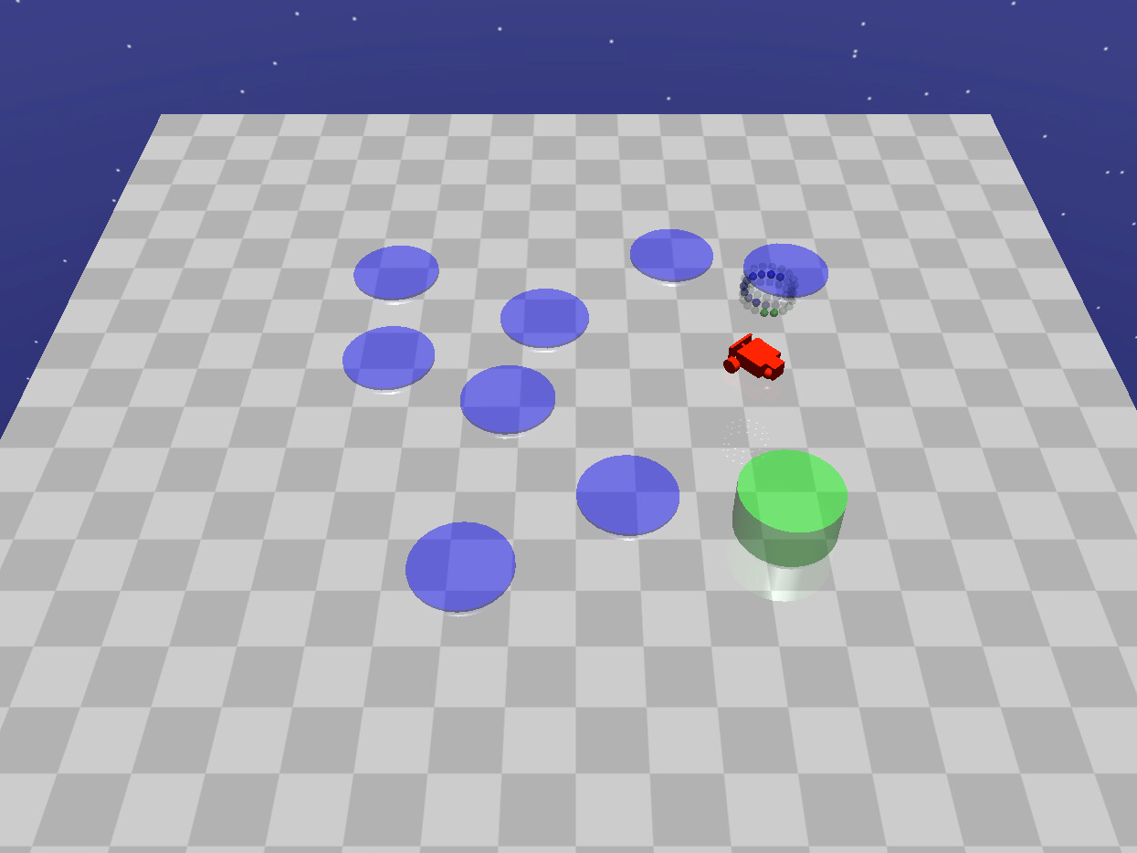
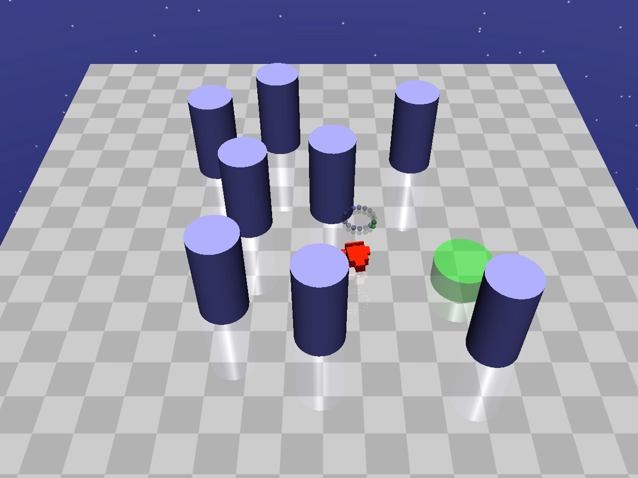
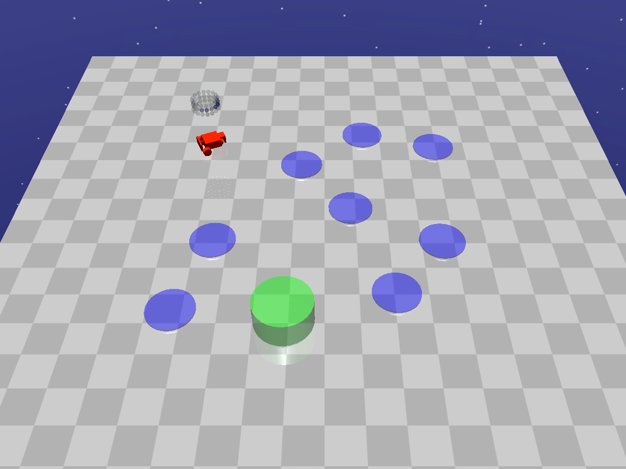
[Hazards: non-physical dangerous areas.] [Pillars: Static physical obstacles] [Goal task: navigating the robot to reach the green cylinder.] [Push task: pushing the yellow box inside the green cylinder.]

Figure 2: Obstacles and tasks in Safety Gym.

In this section, we use a fine-tuned form of safety index in Zhao et al. (2021)

$$\phi(s)=\sigma+d_{\min}^{n}-d^{n}-k\dot{d}$$ (12)

where $d$ is the distance between the agent and obstacle, $d_{\min}$ is the minimum safe distance, and $\dot{d}$ is the derivative of distance with respect to time, $\xi=[\sigma,n,k]$ are the tunable parameters we desire to optimize in the online synthesis algorithm. The observations in Safety Gym include Lidar, speedometer, and magnetometer, which can be used to compute $d$ and $\dot{d}$ from observations. We compare the proposed algorithm against two types of baseline algorithms:

• CRL baselines, including TRPO-Lagrangian, PPO-Lagrangian and CPO Achiam et al. (2017); Ray et al. (2019). The cost threshold is set at zero to learn solid safe policies.

• FAC with original safety index $\phi_{0}$ and handcrafted safety index $\phi_{h}$, where $\phi_{0}=d_{min}-d$ and $\phi_{h}=0.3+d_{min}^{2}-d^{2}-k\dot{d}$, named as FAC with $\phi_{0}$ and FAC with $\phi_{h}$. The choice of $\phi_{h}$ is based on empirical knowledge. Details about baseline algorithms can be found in Appendix 7.

5.1 Evaluating FAC-SIS and Comparison Analysis

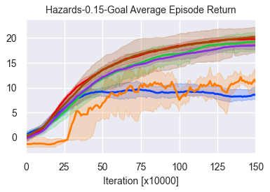
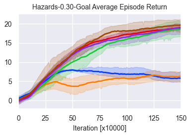
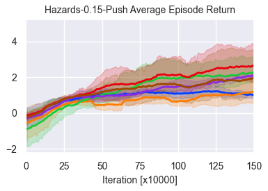
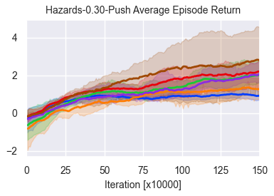
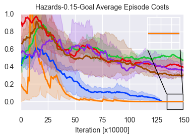
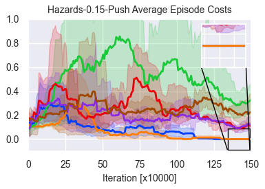
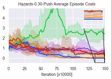
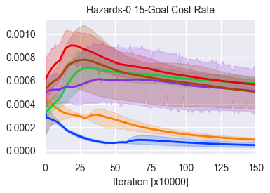
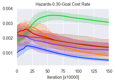
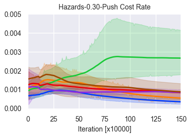
Figure 3: Average performance of FAC-SIS and baseline methods on 4 different Safety Gym environments over five seeds.

Results of the performance comparison are shown in Figure 3. The results suggest that FAC with $\phi_{0}$ performs poorest in the safety performance, which indicates that there are indeed many inevitably unsafe states, and SIS is necessary for these tasks. Only FAC-SIS learns the policy with zero violation and takes the lowest cost rate in all environments, answering the first question of zero constraint violation. FAC with $\phi_{h}$ fails to learn a solid safe policy in those environments with 0.30 constraint size (See the zoomed window in the second row), indicating that the handcrafted safety index can not cover all the environments. As for the baseline CRL algorithms, they can not learn a zero-violation policy in any environment because of the posterior penalty in the trial-and-error mechanism stated above. As for the reward performance, FAC-SIS has comparable reward performance in the Push task. For the Goal task, FAC with $\phi_{h}$ and FAC-SIS sacrifice the reward performance to guarantee safety, explained in Ray et al. (2019).

5.2 Validity Verification of Synthesized Safety Index

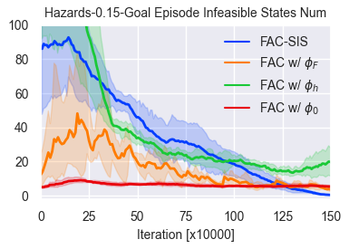
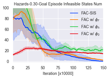
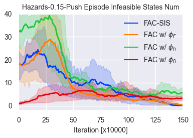
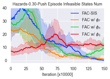
Figure 4: Average episodic number of violations of safe action constraint eq:cstr0. A valid safety index and its corresponding safe control policy should have zero violation performance.

We conduct new metrics and experiments to show the validity of our synthesized safety index. Recall that the validity means that there always exists a feasible control policy to satisfy the constraint in eq:cstr0. To effectively demonstrate the feasibility of SIS, we add a new baseline, FAC with $\phi_{F}$, where $\phi_{F}$ is a valid safety index verified by Zhao et al. (2021). Figure 4 demonstrates the episodic number of constraint violations of eq:cstr0 in the Safety Gym environments. The results show that FAC-SIS and FAC with $\phi_{F}$ can reach a nearly stable zero violation, which means that FAC can satisfy safe action constraint for a given valid safety index, and FAC-SIS also synthesizes a valid safety index. However, with $\phi_{0}$ and $\phi_{h}$ there are consistent violations even with the converged policy, caused by different reasons. For $\phi_{h}$, the reason is simply the inability to make the energy dissipate. For $\phi_{0}$, no high-order derivative in the safety index, so $\phi_{0}$ cannot handle the high relative-degree between the constraint function and control input.

Furthermore, we want to give some scalable analyses about SIS. Firstly, we want to visualize that we can always find actions to dissipate the energy in the sampled distributions after SIS. We conduct experiments on a simple collision-avoidance environment shown in fig:statedist. We select three different initialization rules of the agent and hazard. We use a sample-based exhaustive method to identify infeasible states and see if they overlap the sampled state distributions. We project the state distribution to the 2D space of $d$ and $\dot{d}$, and the results are listed in Figure 7. As we expect all the sampled states to be feasible, these two distributions should not overlap. The results show that the overlap of these two distributions is very small, which indicates that nearly all the sampling states are feasible.

Secondly, we want to visualize the shape of the safe set concerning the learned safety index. We slice the state space into three 2D planes with different agent heading angles, as shown in fig:shape. We use Hamilton-Jacobi reachability analysis to compute the avoidable sets numerically. The avoidable set considers the safe set under the most conservative control inputs, which is the maximum controlled invariant set (Mitchell, 2007; Choi et al., 2021). We use $\phi_{h}$ as the initial safety index of SIS. fig:shape demonstrates that inevitable unsafe states exist in the zero-sublevel set of the empirical safety index. It also shows that we successfully exclude the inevitably unsafe sets through SIS. Notably, the zero-sublevel sets of the synthesized safety index are the subsets of the HJ-avoidable sets. The reasons why SIS can not learn the perfect shapes include limits of the representation capabilities of the safety index parameterization. Additionally, we still consider the optimal criteria, resulting in less conservative policies and possibly smaller safe sets.

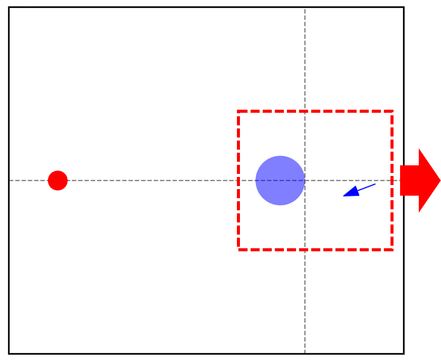
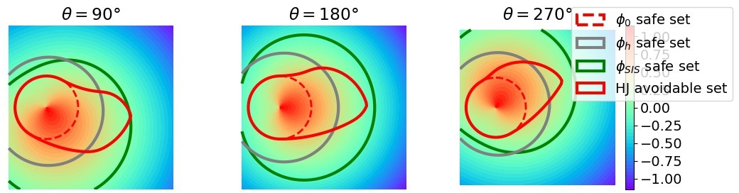
Figure 5: The color indicates the value of the synthesized safety index. The zero-sublevel set of learned safety index is a subset of the numerically max forward invariant set, the HJ avoidable set. We exclude all inevitably unsafe states through SIS like fig:intro. HJ-based solution is only capable for goal-reaching tasks with the reach-avoid problem formulation, while proposed algorithm can handle arbitrary task.

6 Conclusion

This paper focuses on the joint synthesis of the safety certificate and the safe control policy for unknown dynamical systems and general tasks using a CRL approach. We are the first study to start with unknown dynamics and imperfect safety certificates, which significantly improves the applicability of the energy-function-based safe control. We add the optimization of safety index parameters as an outer loop of Lagrangian-based CRL with a unified loss. The convergence is analyzed theoretically. Experimental results demonstrate that the proposed FAC-SIS synthesizes a valid safe index while learning a safe control policy. In future work, we will consider more complex safety index parameterization rules, for example, neural networks. Meanwhile, we will consider other factors in SIS, such as the reward performance of the safe control policies. This work was done during Haitong Ma’s internship at Carnegie Mellon University. This study is supported by National Key R&D Program of China with 2020YFB1600602 and Tsinghua University-Didi Joint Research Center for Future Mobility. This study is also supported by Tsinghua-Toyota Joint Research Fund. The authors would like to thank Mr. Weiye Zhao and Mr. Tianhao Wei for their valuable suggestions on the experiments.

Appendix A Theoretical Results in Section 3

A.1 Proof of Lemma 3.2

Define set of states with safe actions as $\mathcal{S}_{f}=\{s|\mathcal{U}_{s}(s)\neq\emptyset\}$. $\Delta=\mathbb{E}_{s}\{-v^{\pi^{*}}(s)\}$ since $-v^{\pi}(s)$ is irrelevant with $\phi$. For $s\notin\mathcal{S}_{f}$ (i.e., $\big{(}\phi(s^{\prime})-\max\{\phi(s)-\eta_{D},0\}\big{)}>0$), we know that $\lambda^{*}(s)\to\infty$ from Lemma 3.1. Then $\lambda^{*}(s)$ is clipped to $\lambda_{\max}$. Therefore, the Lagrange function $\eqref{eq:lagwithphi}$ can be reformulated to

$$\aligned&\mathcal{L}^{\prime}(\pi^{*},\lambda^{*},\phi)\\ =\left.\mathbb{E}_{s}\Big{\{}-v^{\pi}(s)+\lambda^{*}(s)\big{(}\phi(s^{\prime})-\max\{\phi(s)-\eta_{D},0\}\big{)}\Big{\}}\right|_{\pi=\pi^{*}}\\ =\left.\mathbb{E}_{s}\Big{\{}\lambda^{*}(s)\big{(}\phi(s^{\prime})-\max\{\phi(s)-\eta_{D},0\}\big{)}\Big{\}}\right|_{\pi=\pi^{*}}+\Delta\\ =\left.\mathbb{E}_{s\notin\mathcal{S}_{f}}\Big{\{}\lambda^{*}(s)\big{(}\phi(s^{\prime})-\max\{\phi(s)-\eta_{D},0\}\big{)}\Big{\}}\right|_{\pi=\pi^{*}}+\Delta\\ =\left.\lambda_{\max}\mathbb{E}_{s\notin\mathcal{S}_{f}}\Big{\{}\big{(}\phi(s^{\prime})-\max\{\phi(s)-\eta_{D},0\}\big{)}\Big{\}}\right|_{\pi=\pi^{*}}+\Delta\\ =\lambda_{\max}J(\phi)+\Delta\notag$$ (13)

Appendix B Theoretical Results in Section 4

B.1 Gradients Computation

The objective function of updating the policy and multipliers is the Lagrange function eq:SL2. Using the framework of maximum entropy RL, the objective function of policy update is:

$$J_{\pi}(\theta)=\mathbb{E}_{{s_{t}}\sim\mathcal{D}}\bigg{\{}\mathbb{E}_{\and\sim\pi_{\theta}}\Big{\{}\alpha\log\big{(}\pi_{\theta}\left(\and\mid{s_{t}}\right)\big{)}-Q_{w}({s_{t}},\and)+\lambda_{\xi}({s_{t}})Q_{\phi}({s_{t}},\and)\Big{\}}\bigg{\}}\notag$$ (14)

The policy gradient with the reparameterized policy $\and=f_{\theta}(\epsilon_{t};{s_{t}})$ can be approximated by:

$$\aligned G_{\theta}=\hat{\nabla}_{\theta}J_{\pi}(\theta)=&\nabla_{\theta}\alpha\log\big{(}\pi_{\theta}\left(\and\mid{s_{t}}\right)\big{)}+\Big{(}\nabla_{\and}\alpha\log\left(\pi_{\theta}\left(\and\mid{s_{t}}\right)\right)\\ -\nabla_{\and}\big{(}Q_{w}\left({s_{t}},\and\right)-\lambda_{\xi}({s_{t}})Q_{\phi}\left({s_{t}},\and\right)\big{)}\Big{)}\nabla_{\theta}f_{\theta}\left(\epsilon_{t};{s_{t}}\right)$$

where $\hat{\nabla}_{\theta}J_{\pi}(\theta)$ represents the stochastic gradient with respect to $\theta$, and $Q_{\phi}(s_{t},a_{t})=\big{(}\phi({s_{t+1}})-\max\{\phi({s_{t}})-\eta_{D},0\}\big{)}$. Neglecting those irrelevant parts, the objective function of updating the multiplier network parameters $\xi$ is

$$J_{\lambda}(\xi)=\mathbb{E}_{{s_{t}}\sim\mathcal{D}}\bigg{\{}\mathbb{E}_{\and\sim\pi_{\theta}}\Big{\{}\lambda_{\xi}({s_{t}})\big{(}Q_{\phi}({s_{t}},\and)-d\big{)}\Big{\}}\bigg{\}}$$

The stochastic gradient is

$$G_{\xi}=\hat{\nabla}J_{\lambda}(\xi)=Q_{\phi}({s_{t}},\and)\nabla_{\xi}\lambda_{\xi}({s_{t}})$$ (15)

The objective function of updating the safety index parameters $\zeta$ is already discussed, so the gradients for $\zeta$ is

$$G_{\zeta}=\lambda_{\xi}({s_{t}})\nabla_{\zeta}\Delta\phi^{\pi_{\theta}}({s_{t}})$$ (16)

where $\Delta\phi^{\pi_{\theta}}({s_{t}})=\big{(}\phi({s_{t+1}})-\max\{\phi({s_{t}})-\eta_{D},0\}\big{)}|_{\pi_{\theta}}$, we use a different notation from $Q_{\phi}({s_{t}},\and)$ since we focus on different variables.

B.2 Proof of Theorem 4.3

Recall the overview of the total convergence proof:

1. First we show that each update of the multi-time scale discrete stochastic approximation algorithm $(\theta_{k},\xi_{k},\zeta_{k})$ converges almost surely, but at different speeds, to the stationary point $(\theta^{*},\xi^{*},\zeta^{*})$ of the corresponding continuous-time system.

2. By Lyapunov analysis, we show that the continuous time system is locally asymptotically stable at $(\theta^{*},\xi^{*},\zeta^{*})$.

3. We prove that $(\theta^{*},\xi^{*})$ is the locally optimal solution, or a local saddle point for the CRL problems with local optimal safety index parameters $\zeta^{*}$.

First, we introduce the important lemma used for the convergence proof:

Lemma B.1 (Soft policy evaluation, Haarnoja et al. (2018b)).

The Q-function update will converge to the soft Q-function as the iteration number goes to infinity.

Remark B.2.

In stochastic programming, the error in policy improvement caused by Q-function is a fixed bias rather than random variables, resulting in that it will not affect the convergence as long as the error is bounded. Therefore, we assume that Q-function is fully updated here for simplicity. Otherwise, the proof will be wordy.

Lemma B.3 (Convergence of clipped SGD, Zhang et al. (2019)).

For a stochastic gradient descent problem of a continuous differentiable and $L_{0}-L_{1}$ smooth (which means $\left\|\nabla^{2}f(x)\right\|\leq L_{0}+L_{1}\|\nabla f(x)\|$) loss function $f(x)$ and its stochastic gradient $\hat{\nabla}f(x)$, If these conditions are satisfied

1. $f(x)$ is lower bounded;

2. There exists $\tau>0$, such that $\|\nabla\hat{f}(x)-\nabla f(x)\|\leq\tau$ almost surely;

then the update of stochastic gradient descent converges almost surely with finite iteration complexity.

Then we continue to finish the multi-timescale convergence:

Remark B.4.

In each timescale, we prove two facts, (1) the stochastic error is bounded, so the clipped gradient descent will converge. (2) the converged point is a stationary point. (Bhatnagar et al., 2009; Bhatnagar and Lakshmanan, 2012; Chow et al., 2017).

Timescale 1 (Convergence of $\theta$ update).

Bounded error. As the random variable $G_{\theta}$ depends on the state-action pair sampled from replay buffer, so in the following derivation, it is denoted as $G_{\theta}(s,a)$. For the SGD using sampled $(s_{k},a_{k})$ at $k^{\text{th}}$ step, the stochastic gradient is denoted by $G_{\theta_{k}}(s_{k},a_{k})$. The error term with respect to $\theta$ is computed by

$$\aligned\delta\theta_{k}=G_{\theta_{k}}(s_{k},a_{k})-\mathbb{E}_{s\sim f^{\pi_{\theta}}}\big{\{}\mathbb{E}_{a\sim\pi_{\theta}}G_{\theta_{k}}(s,a)\big{\}}$$ (17)

Therefore, the error term is bounded by

$$\aligned&\left\|\delta\theta_{k}\right\|^{2}\\ \leq 2\left\|f^{\pi_{\theta}}(s)\pi(a|s)\right\|_{\infty}^{2}\left(\left\|G_{\theta_{k}}(s,a)\right\|_{\infty}^{2}+|G_{\theta_{k}}(s_{k},a_{k})|^{2}\right)\\ \leq 6\left\|f^{\pi_{\theta}}(s)\pi(a|s)\right\|_{\infty}^{2}\left\|G_{\theta_{k}}(s,a)\right\|_{\infty}^{2}$$ (18)

where $f^{\pi_{\theta}}$ is the state distribution density under $\pi_{\theta}$. As we assume the state and action are sampled from a closed set and the continuity of neural network, the upper bound is valid. According to Lemma B.3 and invoking Theorem 2 in Chapter 2 of Borkar’s book Borkar (2009), the optimization converges to a fixed point $\theta^{*}$ almost surely (for given $\xi,\zeta$).

Stationary point $\theta^{*}$. Then we show that the fixed point $\theta^{*}$ is a stationary point using Lyapunov analysis. The analysis of the fastest timescale, $\theta$ update, is rather easy, but it is helpful for the similar analyses in the next two timescales. According to Borkar (2009), we can regard the stochastic optimization of $\theta$ as a stochastic approximation of a dynamic system for given $\xi,\zeta$:

$$\dot{\theta}=-\nabla_{\theta}\mathcal{L}^{\prime}(\theta,\xi,\zeta)$$ (19)

Proposition B.5.

consider a Lyapunov function for dynamic system eq:odetheta:

$$L_{\xi,\zeta}(\theta)=\mathcal{L}^{\prime}\left(\theta,\xi,\zeta\right)-\mathcal{L}^{\prime}\left(\theta^{*}(\xi,\zeta),\xi,\zeta\right)$$ (20)

where $\theta^{*}(\xi,\zeta)$ is a local minimum for given $\xi,\zeta$. In order to show that $\theta^{*}$ is a stationary point, we need

$$dL_{\xi,\zeta}(\theta)/dt\leq 0$$ (21)

Proof B.6.

We have

$$\frac{dL_{\xi,\zeta}(\theta)}{dt}=-\left\|\nabla_{\theta}\mathcal{L}^{\prime}(\theta,\xi,\zeta)\right\|^{2}\leq 0$$ (22)

The equality holds only when $\mathcal{L}^{\prime}(\theta,\xi,\zeta)=0$.

Combined with the conclusion of convergence, $\{\theta_{k}\}$ converges almost surely to a local minimum point $\theta^{*}$ for given $\xi$.

Timescale 2 (Convergence of $\lambda$ update).

Bounded Error.

The error term of the $\xi$ update,

$$G_{\xi_{k}}(s_{k},a_{k})-\mathbb{E}_{s}\big{\{}\mathbb{E}_{a}G_{\xi_{k}}(s,a)\big{\}}$$ (23)

includes two parts:

1. $\delta\theta_{\epsilon}$ cased by inaccurate update of $\theta$ ($\theta$ should converge to $\theta^{*}(\xi,\zeta)$ in Timescale 1, but to $\theta_{k}$ near $\theta^{*}(\xi,\zeta)$):

   $$\aligned\delta\theta_{\epsilon}=&{\hat{\nabla}}_{\xi}\mathcal{L}^{\prime}(\theta_{k},\xi,\zeta)-{\hat{\nabla}}_{\xi}\mathcal{L}^{\prime}(\theta^{*}(\xi,\zeta),\xi,\zeta)\\ =\left(Q^{\pi_{\theta_{k}}}(s_{k},a_{k})-Q^{\pi_{\theta^{*}}}(s_{k},a_{k})\right)\nabla_{\xi}\lambda_{\xi}(s_{k})\\ =\left(\nabla_{a}Q(s_{k},a_{k})\nabla_{\theta}\pi(s_{k})\epsilon_{\theta_{k}}+o(\left\|\epsilon_{\theta_{k}}\right\|)\right)\nabla_{\xi}\lambda_{\xi}(s_{k})$$ (24)

   Therefore, $\|\delta\theta_{\epsilon}\|\to 0$ as $\|\epsilon_{\theta}\|\to 0$. The error is bounded since $\|\epsilon_{\theta}\|$ is a small error, where there must exists a positive scalar $\epsilon_{0}$ s.t. $\|\epsilon_{\theta}\|\leq\epsilon_{0}$.

2. $\delta\xi_{k}$ caused by estimation error of $\xi$:

   $$\delta\xi_{k}=G_{\xi_{k}}(s_{k},a_{k})-\mathbb{E}_{s\sim f^{\pi_{\theta}}}\big{\{}\mathbb{E}_{a\sim\pi_{\theta}}G_{\xi_{k}}(s,a)\big{\}}$$ (25)

   $$\left\|\delta\xi_{k}\right\|^{2}\leq 4\left\|f^{\pi_{\theta}}(s)\pi(a|s)\right\|_{\infty}^{2}\left(\max\left\|Q_{\phi}\left(s,a\right)\right\|^{2}+d^{2}\right)\left\|\nabla_{\xi}\lambda_{\xi}(s_{t})\right\|_{\infty}^{2}$$ (26)

   Similar to the analysis of Timescale 1 with compact domain of $s_{k}$, we can get the valid upper bound.

We again use Lemma B.3 and Theorem 2 in Chapter 6 in Borkar (2009) to show that the sequence $\{\xi_{k}\}$ converges to the solution of the following ODE:

$$\dot{\xi}=-\nabla_{\xi}\mathcal{L}^{\prime}(\theta^{*}(\xi,\zeta),\xi,\zeta)$$ (27)

Stationary point. Then we show that the fixed point $\xi^{*}$ is a stationary point using Lyapunov analysis. Note that we have to take $\epsilon_{\theta}$ into considerations.

Proposition B.7.

For the dynamic system with the error term

$$\dot{\xi}=-\nabla_{\xi}\mathcal{L}^{\prime}(\theta^{*}(\xi,\zeta)+\epsilon_{\theta},\xi,\zeta)$$ (28)

Define a Lyapunov function to be

$$L_{\zeta}(\xi)=\mathcal{L}^{\prime}(\theta^{*}(\xi,\zeta),\xi,\zeta)-\mathcal{L}^{\prime}\left(\theta^{*}(\xi,\zeta),\xi^{*}(\zeta),\zeta\right)$$ (29)

where $\xi^{*}$ is a local maximum point. Then $\frac{dL_{\zeta}(\xi)}{dt}\leq 0$.

Proof B.8.

The proof is similar to Proposition 2; only the error of $\theta$ should be considered. We prove that the error of $\theta$ does not affect the decreasing property here:

$$\aligned&\frac{dL_{\zeta}(\xi)}{dt}=-\left(\nabla_{\xi}\mathcal{L}^{\prime}(\theta^{*}(\xi,\zeta)+\epsilon_{\theta},\xi,\zeta)\right)^{T}\nabla_{\xi}\mathcal{L}^{\prime}(\theta^{*}(\xi,\zeta),\xi,\zeta)\\ =-\left\|\nabla_{\xi}\mathcal{L}^{\prime}(\theta^{*}(\xi,\zeta),\xi,\zeta)\right\|^{2}-\delta\theta_{\epsilon}^{T}\nabla_{\xi}\mathcal{L}^{\prime}(\theta^{*}(\xi,\zeta),\xi,\zeta)\\ \leq-\left\|\nabla_{\xi}\mathcal{L}^{\prime}(\theta^{*}(\xi,\zeta),\xi,\zeta)\right\|^{2}+K_{1}\left\|\epsilon_{\theta}\right\|\left\|\nabla_{\xi}\mathcal{L}^{\prime}(\theta^{*}(\xi,\zeta),\xi,\zeta)\right\|\\$$ (30)

where $K_{1}=\|\nabla_{a}Q(s_{k},a_{k})\nabla_{\theta}\pi(s_{k})\epsilon_{\theta_{k}}\|_{\infty}\|\nabla_{\xi}\lambda_{\xi}(s_{k})\|_{\infty}\leq\infty$ according to eq:thetaerrorts2 since the compact domain of $s_{k},a_{k}$ according to Assumption 2. As $\theta$ converges much faster than $\xi$ according to the multiple timescale convergence in Borkar (2009), we get $dL_{\zeta}(\xi)/dt\leq 0$. Therefore, there exists trajectory $\xi(t)$ converges to $\xi^{*}$ if initial state $\xi_{0}$ starts from a ball $\mathcal{D}_{\xi^{*}}$ around $\xi^{*}$ according to the asymptotically stable systems.

Local saddle point of $(\theta^{*},\xi^{*})$. One side of the saddle pioint, $\mathcal{L}^{\prime}(\theta^{*}(\xi,\zeta),\xi^{*}(\zeta),\zeta)\leq\mathcal{L}^{\prime}\left(\theta,\xi^{*}(\zeta),\zeta\right)$ are already provided in previous, so we need to prove here $\mathcal{L}^{\prime}\left(\theta^{*}(\xi,\zeta),\xi^{*}(\zeta),\zeta\right)\geq\mathcal{L}^{\prime}\left(\theta^{*}(\xi,\zeta),\xi,\zeta\right)$. To complete the proof we need that

$$Q_{\phi}(s,a)\leq d\text{and}\lambda^{*}(s)(Q_{\phi}(s,a)-d)=0$$ (31)

for all $s$ in $\mathcal{S}_{f}$, and $a$ sampled from $\pi_{\theta^{*}(\xi,\zeta)}$. Recall that $\lambda^{*}$ is a local maximum point, we have

$$\nabla_{\xi}\mathcal{L}^{\prime}\left(\theta^{*}(\xi,\zeta),\xi^{*}(\zeta),\zeta\right)=0$$ (32)

Assume there exists $s_{t}$ and action $a_{t}$ sampled from $\pi^{*}(s_{t})$ so that $Q_{\phi}(s_{t},a_{t})>0$. Then for $\lambda^{*}$ we have

$$\nabla_{\xi}\mathcal{L}^{\prime}\left(\theta^{*}(\xi,\zeta),\xi^{*}(\zeta),\zeta\right)=d_{\gamma}^{\pi_{\theta}^{*}}(s_{t})Q_{\phi}(s_{t},a_{t})\nabla_{\xi}\lambda_{\xi}(s_{t})\neq 0$$ (33)

The second part only requires that $\lambda^{*}(s_{t})=0$ when $Q_{\phi}(s_{t},a_{t})<0$. Similarly, we assume that there exists $s_{t}$ and $\xi^{*}$ where $\lambda_{\xi^{*}}(s_{t})>0$ and $Q_{\phi}(s_{t},a_{t})<d$. there must exists a $\xi_{0}$ subject to

$$\xi_{0}=\xi^{*}+\eta_{0}f^{\pi_{\theta^{*}}}(s_{t})\left(Q_{\phi}(s_{t},a_{t})-d\right)\nabla_{\xi}\lambda_{\xi}(s_{t})$$ (34)

for any $\eta\in(0,\eta_{0}]$ where $\eta_{0}\geq 0$. It contradicts the statement the local maximum $\xi^{*}$. Then we get

$$\aligned&\mathcal{L}^{\prime}\left(\theta^{*}(\xi,\zeta),\xi^{*}(\zeta),\zeta\right)\\ =J_{r}(\theta^{*})+\mathbb{E}_{s}\left\{\lambda_{\xi^{*}}(s)\mathbb{E}_{a\sim\pi}\{Q_{\phi}(s,a)\}\right\}=J_{r}(\theta^{*})\\ \geq J_{r}(\theta^{*})+\mathbb{E}_{s}\left\{\lambda_{\xi}(s)\mathbb{E}_{a\sim\pi}\{Q_{\phi}(s,a)\}\right\}\\ =\mathcal{L}^{\prime}\left(\theta^{*}(\xi,\zeta),\xi,\zeta\right)$$ (35)

So $(\theta^{*},\xi^{*})$ is a locally saddle point for given safety index parameters $\zeta$.

Timescale 3 (Convergence of $\zeta$ update).

Bounded error. Similar to Timescale 2, the error of $\zeta$ update includes two parts

1. $\delta\theta_{\epsilon}+\delta\xi_{\epsilon}$ caused by inaccurate update of $\theta,\xi$:

   $$\aligned&\delta\theta_{\epsilon}+\delta\xi_{\epsilon}\\ =\lambda_{\xi_{k}}(s_{k})\nabla_{\xi}\Delta\phi^{\pi_{\theta_{k}}}(s_{k})-\lambda_{\xi^{*}}(s_{k})\nabla_{\zeta}\Delta\phi^{\pi_{\theta^{*}}}(s_{k})\\ =\lambda_{\xi_{k}}(s_{k})\nabla_{\zeta}\Delta\phi^{\pi_{\theta_{k}}}(s_{k})-\lambda_{\xi_{k}}(s_{k})\nabla_{\zeta}\Delta\phi^{\pi_{\theta^{*}}}(s_{k})\\ +\lambda_{\xi_{k}}(s_{k})\nabla_{\zeta}\Delta\phi^{\pi_{\theta^{*}}}(s_{k})-\lambda_{\xi^{*}}(s_{k})\nabla_{\zeta}\Delta\phi^{\pi_{\theta^{*}}}(s_{k})\\ =\left(\lambda_{\xi_{k}}(s_{k})-\lambda_{\xi^{*}}(s_{k})\right)\nabla_{\zeta}\Delta\phi^{\pi_{\theta^{*}}}(s_{k})$$ (36)

   The first part after the second equal sign is neglected since $\theta$ permutation does not affect on the gradient of $\zeta$. Similar to derivation in eq:thetaerrorts2, we get $|\delta\theta_{\epsilon}+\delta\xi_{\epsilon}|\rightarrow 0$ as $(\theta,\xi)\rightarrow(\theta^{*},\xi^{*})$.

2. $\delta\zeta_{k}$ caused by estimation error of $\zeta$:

   $$\delta\zeta_{k}=\lambda_{\xi^{*}}(s_{k})\nabla_{\zeta}\Delta\phi^{\pi_{\theta^{*}}}(s_{k})-\mathbb{E}\left\{\lambda_{\xi^{*}}(s)\nabla_{\zeta}\Delta\phi^{\pi_{\theta^{*}}}(s)\right\}$$ (37)

   The bounded error can be obtained by

   $$\aligned&\left\|\delta\zeta_{k}\right\|^{2}\\ \leq 4\left\|f^{\pi_{\theta}}(s)\pi(a|s)\right\|_{\infty}^{2}\max_{s\in\complement_{\mathcal{D}}\mathcal{S}_{f}}|\lambda_{\xi^{*}}(s)|^{2}\|\nabla_{\zeta}\Delta\phi^{\pi_{\theta^{*}}}(s)\|^{2}\\$$ (38)

Therefore, the $\zeta$-update is a stochastic approximation of the continuous system $\zeta(t)$, described by the ODE For the dynamic system

$$\dot{\zeta}=-\nabla_{\zeta}\mathcal{L}^{\prime}(\theta,\xi,\zeta)|_{\theta=\theta^{*}(\xi,\zeta)+\epsilon_{\theta},\xi=\xi^{*}(\zeta)+\epsilon_{\xi}}$$ (39)

Stationary point. Define a Lyapunov function

$$L(\zeta)=\mathcal{L}^{\prime}\left(\theta^{*}(\xi,\zeta),\xi^{*}(\zeta),\zeta\right)-\mathcal{L}^{\prime}\left(\theta^{*},\xi^{*},\zeta^{*}\right)$$ (40)

where $\zeta^{*}\in Z$ is a local minimum point. Then

$$\aligned&\frac{dL(\zeta)}{dt}\\ =\small{\left(-\nabla_{\zeta}\mathcal{L}^{\prime}(\theta^{*}(\xi,\zeta)+\epsilon_{\theta},\xi^{*}(\zeta)+\epsilon_{\xi},\zeta)\right)^{T}\nabla_{\zeta}\mathcal{L}^{\prime}(\theta^{*}(\xi,\zeta),\xi^{*}(\zeta),\zeta)}\\ \leq-\left\|\nabla_{\zeta}\mathcal{L}^{\prime}(\theta^{*}(\xi,\zeta),\xi^{*}(\zeta),\zeta)\right\|^{2}\\ +K_{2}\left\|\epsilon_{\xi}\right\|\left\|\nabla_{\zeta}\mathcal{L}^{\prime}(\theta^{*}(\xi,\zeta),\xi^{*}(\zeta),\zeta)\right\|$$ (41)

where $K_{2}=\|\nabla_{\xi}\lambda_{\xi}(s)\|_{\infty}\|\nabla_{\zeta}\Delta\phi^{\pi_{\theta^{*}}}(s)\|_{\infty}$ according to eq:zetaerror. The derivation is very similar to the conclusion in Proposition B.7; the upper bound is valid since the compact domain of state and action. As $\xi$ converges faster than $\zeta$, $dL_{\zeta}(\xi)/dt\leq 0$, so there exists trajectory $\xi(t)$ converges to $\zeta^{*}$ if initial state $\zeta_{0}$ starts from a ball $\mathcal{D}_{\zeta^{*}}$ around $\zeta^{*}$ according to the asymptotically stable systems.

Finally, we can conclude that the sequence $(\theta_{k},\xi_{k},\zeta_{k})$, will converge to a locally optimal policy and multiplier tuple $(\theta^{*},\xi^{*})$ for a locally optimal safety index parameters, $\zeta^{*}$.

Appendix C Implementation Details

C.1 Codebase and Platforms

Implementation of FAC-SIS, FAC with $\phi_{h}$ and $\phi_{F}$ are based on the Parallel Asynchronous Buffer-Actor-Learner (PABAL) architecture proposed by Duan et al. (2021). All experiments are implemented on Intel Xeon Gold 6248 processors with 12 parallel actors, including 4 workers to sample, 4 buffers to store data and 4 learners to compute gradients. Implementation of other baseline algorithms are based on the code released by Ray et al. (2019) and also a modified version of PPO.

C.2 Baseline Algorithms

The only difference between baseline algorithms, FAC with $\phi_{h},\ \phi_{F}$ is that no $\zeta$ update step in Algorithm 1.

Appendix D Hyperparameters

The neural network design and detailed hyperparameters are listed in Table 4.

Appendix E Additional Experimental Results

E.1 Experiments in Other Safety Gym environments

We select six different Safety Gym environments, and the results of four of them are listed in the experiment section. The results with the rest of the environments are demonstrated here:

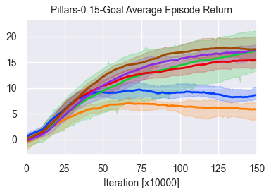
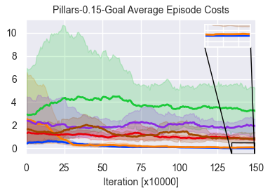
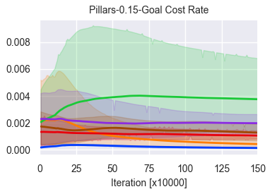
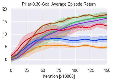
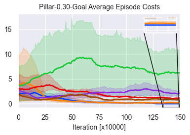
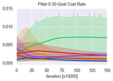
Figure 6: Average performance of FAC-SIS and baseline methods on 2 additional Safety Gym environments over five seeds.

The results in the other two environments are consistent with the experiment section. The proposed FAC-SIS learns a safe policy with zero constraint violation, and other baseline algorithms all fail to neglect the cost even in the converged policies. Furthermore, the reward performance is better than the handcrafted safety index, or FAC with $\phi_{h}$.

E.2 Custom Environment Details

To effectively scale the state distribution, we manually set an environment similar to the Safety Gym environments with Point robot, Goal task and Hazard obstacles shown in Figure 7. The agent represented by the arrow should head to the red dot on the top while avoiding the hazard randomly located near the origin. The custom environment includes a static goal point at $(0,5)$, a hazard with a radius of 0.5, and a point agent with two inputs, rotation and acceleration, the arrow represents the positive direction of the acceleration. The random initial positions (including positions, heading angles of the agent and the positions of hazard) design of three different distributions are listed in Table 1. The reward design includes two parts that are the tracking error of the heading angle towards goal position, and speed relevant to the distance to the goal position (It requires that the agent always takes 5 seconds to reach the goal, so the closer the agent get to the goal, the slower its target speed is.).

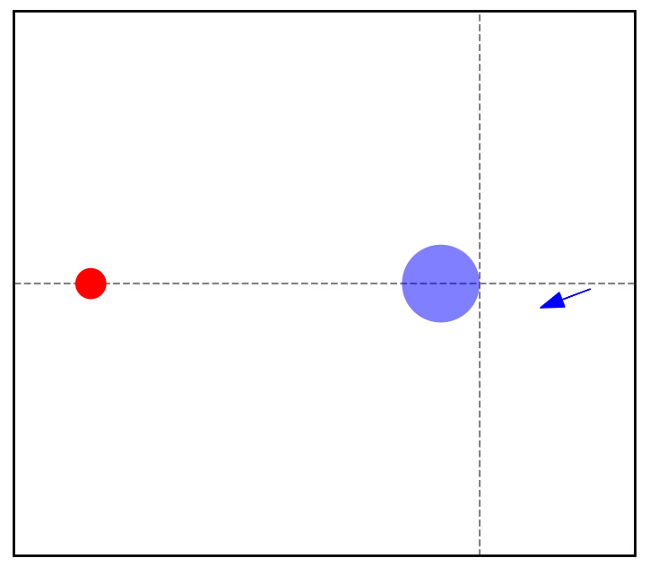
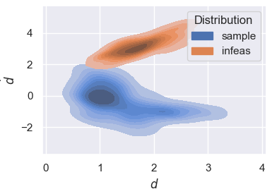
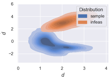
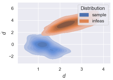
Figure 7: The custom environment and distributions of sampling and infeasible states under three different initialization setups. The overlap of the two distributions is very small, indicating that safe control exists for almost all sampled states.

The method to locate infeasible states is explained as follows. First, we discretize the state and action space with small intervals, and we exhaust all the actions to see if the energy can dissipate for each state. If not, we remark the specific state as infeasible.

Distribution Index	Agent Initial Position			Hazard Initial Position
	x	y	Angle	x	y
1	$0$	$[-1.5,-1.0]$	$[-\pi/4,\pi/4]$	$0$	$[0.5,1]$
2	$0$	$[-1.5,-0.5]$	$[-\pi/4,\pi/4]$	$0$	$[0.5,1,5]$
3	$[-0.5,0.5]$	$[-1.5,-0.5]$	$[-\pi/4,\pi/4]$	$0$	$[0.5,1]$

Table 1: Initial distribution in custom environments. The initial position is sampled with a uniform distribution between the interval in the table.

E.3 Additional Results for Safety Index Synthesis

Parameters	Notion	$k$	$\sigma$	$n$
Synthesized	$\phi_{SIS}$	0.7821	0.0958	1.149
Handcrafted	$\phi_{h}$	1	0.3	2
Feasible	$\phi_{F}$	1	0.04	2
Zero	$\phi_{0}$	0	0	1

Table 2: Parameterization of Different Safety Index.

We list the different safety index parameters in TABLE 2. To be more specific, FAC-SIS has a single-direction update of the parameters by reducing the $k,\sigma$ and changing $n$ as shown in Figure 8.

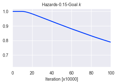
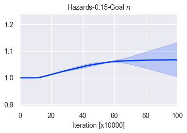
Figure 8: Learning curves of safety index parameters.

The trend can be explained by these two cases:

• $\phi(s)\leq 0$. Then the constraints, or the violation part are

  $$\phi(s^{\prime})=\sigma+d_{min}^{n}-d^{n}-k\dot{d}\leq 0$$ (42)

  Therefore, if we want to further optimize the violation part $J_{\phi}$, or the sum of LHS of the inequality in eq:case1, then we have:

  $$\begin{array}[]{l}\partial J_{\phi}/\partial\sigma=1>0\\ \partial J_{\phi}/\partial n=n(d_{min}^{n-1}-d^{n-1})<0\\ \partial J_{\phi}/\partial k=-\dot{d}\end{array}$$ (43)

  So, we should reduce $k$, increase $n$. The trend of $k$ depends on the $\dot{d}$.

• $\phi(s)>0$. If we further let $\eta_{D}=0$, then we have $\phi(s^{\prime})\leq\phi(s)$. The violation part of this inequality constraints are:

  $$d^{n}-d^{\prime n}+k\dot{d}-k\dot{d}^{\prime}$$ (44)

  we have

  $$\begin{array}[]{l}\partial J_{\phi}/\partial\sigma=0\\ \partial J_{\phi}/\partial n=n(d^{n-1}-d^{\prime n-1})\\ \partial J_{\phi}/\partial k=\dot{d}-\dot{d}^{\prime}\end{array}$$ (45)

  As the inequality constraints are violated, so at least there exists one positive term of $(d-d^{\prime})$ and $(\dot{d}-\dot{d}^{\prime})$. In other words, if we want to reduce the violation part eq:case2, whether that one of the $k$ or $n$ reduces, or they all reduce.

Therefore, the synthesis trends in Figure 8 is reasonable.

Metric	$\phi_{0}$	$\phi_{i}$	$\phi_{SIS}$	$\phi_{F}$	$\phi_{h}$
Success rate	0%	85%	99%	100%	70%
$\phi_{0}$ violation rate	100%	0%	0%	0%	0%
Infeasible rate	100%	15%	1%	0%	30%
Average Tracking Error	-	2.974	3.378	3.456	3.528

Table 3: Performance Comparison of Different Safety Indexes.

We add quantified metrics on the custom environment to compare the feasibility, safety, and optimality of different safety indexes shown in TABLE 3. We randomly simulate 100 trajectories to see if the safety index leads to the infeasibility of unsafe actions. If the agent does not violate $\phi_{0}$ (or stepping into hazards) or has infeasible states, then the trajectory is successful. $\phi_{i}$ is the initial safety index before synthesizing, and $\phi_{SIS}$ is the synthesized safety index. They both ensure safety but the $\phi_{SIS}$ increases the feasibility by the safety index synthesis. The $1\%$ difference might be caused by the mismatch of the state distributions between the custom environment and RL environments. $\phi_{F}$ indeed guarantees the best feasibility from the synthesis rules in Zhao et al. (2021). Besides, the synthesized safety index also has slightly better optimality, although we do not intend to improve it. This could be explained by the synthesized safety index being less conservative since it only ensures the sampled region by RL is feasible but not all the state space like the synthesis rules in Zhao et al. (2021).

Algorithm	Value
FAC-SIS, FAC w/ $\phi_{h}$, FAC w/ $\phi_{F}$
Optimizer	Adam ($\beta_{1}=0.9,\beta_{2}=0.999$)
Approximation function	Multi-layer Perceptron
Number of hidden layers	2
Number of hidden units per layer	256
Nonlinearity of hidden layer	ELU
Nonlinearity of output layer	linear
Actor learning rate	Linear annealing $3{\rm{e-}}5\rightarrow 1{\rm{e-}}6$
Critic learning rate	Linear annealing $8{\rm{e-}}5\rightarrow 1{\rm{e-}}6$
Learning rate of multiplier net	Linear annealing $5{\rm{e-}}6\rightarrow 5{\rm{e-}}6$
Learning rate of $\alpha$	Linear annealing $8{\rm{e-}}5\rightarrow 8{\rm{e-}}6$
Learning rate of safety index parameters (FAC-SIS only)	Linear annealing $8{\rm{e-}}6\rightarrow 1{\rm{e-}}6$
Reward discount factor ($\gamma$)	0.99
Policy update interval ($m_{\pi}$)	3
Multiplier ascent interval ($m_{\lambda}$)	12
SIS interval ($m_{\phi}$)	24
Target smoothing coefficient ($\tau$)	0.005
Max episode length ($N$)
Safety Gym task	1000
Custom task	120
Expected entropy ($\overline{\mathcal{H}}$)	$\overline{\mathcal{H}}=-$Action Dimensions
Replay buffer size	$5\times 10^{5}$
Replay batch size	256
Handcrafted safety index ($\phi_{h}$) hyperparameters $(\eta,n,k,\sigma)$	$(0,\ 2,\ 1,\ 0.3)$
Feasible safety index ($\phi_{F}$) hyperparameters $(\eta,n,k,\sigma)$	$(0,\ 2,\ 1,\ 0.04)$
CPO, TRPO-Lagrangian
Max KL divergence	$0.1$
Damping coefficient	$0.1$
Backtrack coefficient	$0.8$
Backtrack iterations	$10$
Iteration for training values	$80$
Init $\lambda$	$0.268(softplus(0))$
GAE parameters	$0.95$
Batch size	$2048$
Max conjugate gradient iterations	$10$
PPO-Lagrangian
Clip ratio	$0.2$
KL margin	$1.2$
Mini Bactch Size	$64$

Table 4: Detailed hyperparameters.

References

- Achiam et al. (2017) Joshua Achiam, David Held, Aviv Tamar, and Pieter Abbeel. Constrained policy optimization. In International Conference on Machine Learning, pages 22–31, Sydney, Australia, 2017. PMLR.
- Agrawal and Sreenath (2017) Ayush Agrawal and Koushil Sreenath. Discrete control barrier functions for safety-critical control of discrete systems with application to bipedal robot navigation. In Robotics: Science and Systems, 2017.
- Ames et al. (2014) Aaron D Ames, Jessy W Grizzle, and Paulo Tabuada. Control barrier function based quadratic programs with application to adaptive cruise control. In 53rd IEEE Conference on Decision and Control, pages 6271–6278. IEEE, 2014.
- Bhatnagar and Lakshmanan (2012) Shalabh Bhatnagar and K Lakshmanan. An online actor–critic algorithm with function approximation for constrained markov decision processes. Journal of Optimization Theory and Applications, 153(3):688–708, 2012.
- Bhatnagar et al. (2009) Shalabh Bhatnagar, Richard S Sutton, Mohammad Ghavamzadeh, and Mark Lee. Natural actor–critic algorithms. Automatica, 45(11):2471–2482, 2009.
- Borkar (2009) Vivek S Borkar. Stochastic approximation: a dynamical systems viewpoint, volume 48. Springer, 2009.
- Chang et al. (2020) Ya-Chien Chang, Nima Roohi, and Sicun Gao. Neural lyapunov control. arXiv preprint arXiv:2005.00611, 2020.
- Chen et al. (2021) Jianyu Chen, Shengbo Eben Li, and Masayoshi Tomizuka. Interpretable end-to-end urban autonomous driving with latent deep reinforcement learning. IEEE Transactions on Intelligent Transportation Systems, 2021.
- Cheng et al. (2019) Richard Cheng, Gábor Orosz, Richard M Murray, and Joel W Burdick. End-to-end safe reinforcement learning through barrier functions for safety-critical continuous control tasks. In Proceedings of the AAAI Conference on Artificial Intelligence, volume 33, pages 3387–3395, 2019.
- Choi et al. (2021) Jason J Choi, Donggun Lee, Koushil Sreenath, Claire J Tomlin, and Sylvia L Herbert. Robust control barrier-value functions for safety-critical control. arXiv preprint arXiv:2104.02808, 2021.
- Chow et al. (2017) Yinlam Chow, Mohammad Ghavamzadeh, Lucas Janson, and Marco Pavone. Risk-constrained reinforcement learning with percentile risk criteria. The Journal of Machine Learning Research, 18(1):6070–6120, 2017.
- Duan et al. (2021) Jingliang Duan, Yang Guan, Shengbo Eben Li, Yangang Ren, Qi Sun, and Bo Cheng. Distributional soft actor-critic: Off-policy reinforcement learning for addressing value estimation errors. IEEE Transactions on Neural Networks and Learning Systems, 2021.
- Fujimoto et al. (2018) Scott Fujimoto, Herke Hoof, and David Meger. Addressing function approximation error in actor-critic methods. In International Conference on Machine Learning, pages 1587–1596, Stockholm, Sweden, 2018. PMLR.
- Gracia et al. (2013) Luis Gracia, Fabricio Garelli, and Antonio Sala. Reactive sliding-mode algorithm for collision avoidance in robotic systems. IEEE Transactions on Control Systems Technology, 21(6):2391–2399, 2013.
- Haarnoja et al. (2018a) Tuomas Haarnoja, Aurick Zhou, Pieter Abbeel, and Sergey Levine. Soft actor-critic: Off-policy maximum entropy deep reinforcement learning with a stochastic actor. In International Conference on Machine Learning, pages 1861–1870, Stockholm, Sweden, 2018a. PMLR.
- Haarnoja et al. (2018b) Tuomas Haarnoja, Aurick Zhou, Kristian Hartikainen, George Tucker, Sehoon Ha, Jie Tan, Vikash Kumar, Henry Zhu, Abhishek Gupta, Pieter Abbeel, et al. Soft actor-critic algorithms and applications. arXiv preprint arXiv:1812.05905, 2018b.
- Jin et al. (2020) Wanxin Jin, Zhaoran Wang, Zhuoran Yang, and Shaoshuai Mou. Neural certificates for safe control policies. arXiv preprint arXiv:2006.08465, 2020.
- Liu and Tomizuka (2014) Changliu Liu and Masayoshi Tomizuka. Control in a safe set: Addressing safety in human-robot interactions. In Dynamic Systems and Control Conference, volume 46209, page V003T42A003. American Society of Mechanical Engineers, 2014.
- Luo and Ma (2021) Yuping Luo and Tengyu Ma. Learning barrier certificates: Towards safe reinforcement learning with zero training-time violations. arXiv preprint arXiv:2108.01846, 2021.
- Ma et al. (2021a) Haitong Ma, Jianyu Chen, Shengbo Eben Li, Ziyu Lin, and Sifa Zheng. Model-based constrained reinforcement learning using generalized control barrier function. arXiv preprint arXiv:2103.01556, 2021a.
- Ma et al. (2021b) Haitong Ma, Yang Guan, Shegnbo Eben Li, Xiangteng Zhang, Sifa Zheng, and Jianyu Chen. Feasible actor-critic: Constrained reinforcement learning for ensuring statewise safety. arXiv preprint arXiv:2105.10682, 2021b.
- Milgrom and Segal (2002) Paul Milgrom and Ilya Segal. Envelope theorems for arbitrary choice sets. Econometrica, 70(2):583–601, 2002.
- Mitchell (2007) Ian M Mitchell. A toolbox of level set methods. UBC Department of Computer Science Technical Report TR-2007-11, 2007.
- Prajna et al. (2007) Stephen Prajna, Ali Jadbabaie, and George J Pappas. A framework for worst-case and stochastic safety verification using barrier certificates. IEEE Transactions on Automatic Control, 52(8):1415–1428, 2007.
- Qin et al. (2021) Zengyi Qin, Kaiqing Zhang, Yuxiao Chen, Jingkai Chen, and Chuchu Fan. Learning safe multi-agent control with decentralized neural barrier certificates. arXiv preprint arXiv:2101.05436, 2021.
- Ray et al. (2019) Alex Ray, Joshua Achiam, and Dario Amodei. Benchmarking safe exploration in deep reinforcement learning. arXiv preprint arXiv:1910.01708, 2019.
- Richter et al. (2019) Florian Richter, Ryan K Orosco, and Michael C Yip. Open-sourced reinforcement learning environments for surgical robotics. arXiv preprint arXiv:1903.02090, 2019.
- Rockafellar (2015) Ralph Tyrell Rockafellar. Convex analysis. Princeton university press, 2015.
- Sallab et al. (2017) Ahmad EL Sallab, Mohammed Abdou, Etienne Perot, and Senthil Yogamani. Deep reinforcement learning framework for autonomous driving. Electronic Imaging, 2017(19):70–76, 2017.
- Saveriano and Lee (2019) Matteo Saveriano and Dongheui Lee. Learning barrier functions for constrained motion planning with dynamical systems. In 2019 IEEE/RSJ International Conference on Intelligent Robots and Systems (IROS), pages 112–119. IEEE, 2019.
- Srinivasan et al. (2020) Mohit Srinivasan, Amogh Dabholkar, Samuel Coogan, and Patricio A Vela. Synthesis of control barrier functions using a supervised machine learning approach. In 2020 IEEE/RSJ International Conference on Intelligent Robots and Systems (IROS), pages 7139–7145. IEEE, 2020.
- Stooke et al. (2020) Adam Stooke, Joshua Achiam, and Pieter Abbeel. Responsive safety in reinforcement learning by pid lagrangian methods. In International Conference on Machine Learning, pages 9133–9143, Online, 2020. PMLR.
- Taylor et al. (2020) Andrew Taylor, Andrew Singletary, Yisong Yue, and Aaron Ames. Learning for safety-critical control with control barrier functions. In Learning for Dynamics and Control, pages 708–717. PMLR, 2020.
- Tessler et al. (2018) Chen Tessler, Daniel J Mankowitz, and Shie Mannor. Reward constrained policy optimization. arXiv preprint arXiv:1805.11074, 2018.
- Uchibe and Doya (2007) Eiji Uchibe and Kenji Doya. Constrained reinforcement learning from intrinsic and extrinsic rewards. In 2007 IEEE 6th International Conference on Development and Learning, pages 163–168, Lugano, Switzerland, 2007. IEEE.
- Wang et al. (2017) Li Wang, Aaron D Ames, and Magnus Egerstedt. Safety barrier certificates for collisions-free multirobot systems. IEEE Transactions on Robotics, 33(3):661–674, 2017.
- Wei and Liu (2019) Tianhao Wei and Changliu Liu. Safe control algorithms using energy functions: A uni ed framework, benchmark, and new directions. In 2019 IEEE 58th Conference on Decision and Control (CDC), pages 238–243. IEEE, 2019.
- Wieland and Allgöwer (2007) Peter Wieland and Frank Allgöwer. Constructive safety using control barrier functions. IFAC Proceedings Volumes, 40(12):462–467, 2007.
- Zhang et al. (2019) Jingzhao Zhang, Tianxing He, Suvrit Sra, and Ali Jadbabaie. Why gradient clipping accelerates training: A theoretical justification for adaptivity. arXiv preprint arXiv:1905.11881, 2019.
- Zhao et al. (2021) Weiye Zhao, Tairan He, and Changliu Liu. Model-free safe control for zero-violation reinforcement learning. In 5th Annual Conference on Robot Learning, 2021.