note-name = , use-sort-key = false

Spin-resolved spectroscopy of helical Andreev bound states

Abstract

We propose a versatile setup that allows performing spin-resolved spectroscopy of helical Andreev bound states, proving their existence and therefore the topological nature of the Josephson junction that hosts them. The latter is realized on the helical edge of a 2D topological insulator, proximitized with two superconducting electrodes. The spectroscopic analysis is enabled by a quantum point contact, which couples the junction with another helical edge acting as a spin-sensitive probe. By means of straightforward transport measurements, it is possible to detect the particular spin structure of the helical Andreev bound state and to shine light on the mechanism responsible for their existence, i.e. the presence of protected Andreev reflection within the Josephson junction. We discuss the robustness of this helical Andreev spectrometer with respect to processes that weaken spin to charge conversion.

Introduction. — Two-dimensional topological insulators (2DTIs) have been receiving a lot of attention since their first discovery König et al. (2007); Bernevig et al. (2006); Kane and Mele (2005a, b) and represent a prominent example of topological systems. They feature a 2D insulating bulk with topologically protected 1D helical edge states, which propagate in opposite directions and have opposite spin orientation Qi and Zhang (2011). Because of this remarkable feature, known as spin-momentum locking, 2DTIs are a precious resource in view of their functionalities in spintronics He et al. (2019); Zhou et al. (2014); Linder and Robinson (2015); Breunig et al. (2018). Moreover, helical edges proximitized by superconductors are predicted to realize topological superconductivity Fu and Kane (2008); Alicea (2012); Sato and Ando (2017), a fundamentally interesting phenomenon with multiple applications, ranging from topological quantum computation Lutchyn et al. (2010); Kitaev (2001); Nayak et al. (2008); Aasen et al. (2016); Oreg et al. (2010) to low-temperature thermal devices Sothmann et al. ; Scharf et al. ; Blasi et al. (2021); Keidel et al. (2020); Gresta et al. (2021). To date, 2DTIs have been proposed and realized in a variety of materials Reis et al. (2017); Shi et al. (2019); Wu et al. (2018); Tang et al. (2017); Li et al. (2018a); Liu et al. (2020); Knez et al. (2011); Liu et al. (2008); Pribiag et al. (2015). One of the most mature platforms is represented by HgTe quantum wells where robust ballistic transport on the edges has been experimentally observed König et al. (2007); Roth et al. (2009); Shamim et al. (2021); Brüne et al. (2012) and superconducting contacts have been successfully fabricated Hart et al. (2014). The latter advancement has allowed for the realization of 2DTI-based Josephson junctions (JJs) and to the subsequent observation of fractional Josephson effect Wiedenmann et al. (2016); Bocquillon et al. (2016, 2018) and superconducting edge transport Hart et al. (2014); Bocquillon et al. (2016).

A distinctive feature of a JJ defined in a 2DTI is the presence of helical Andreev bound states (hABSs) Tkachov and Hankiewicz (2013); Beenakker et al. (2013); Bocquillon et al. (2016); Sothmann and Hankiewicz (2016); Tanaka et al. (2009). They consist of two particular forms of mid-gap states with a specific spin structure and a protected crossing at zero energy. Due to spin-momentum locking and perfect Andreev reflection (AR), each hABS is either a perfect superposition of polarized electrons with spin up and holes with spin down or vice-versa. Their existence represents a hallmark of 2DTI-based JJs and eventually leads to a rich phenomenology, including the theoretically predicted appearance of a zero-energy Majorana Kramers pair Li et al. (2016); Pikulin et al. (2016), as well as the experimentally observed $4\pi$ periodic current-phase relation Laroche et al. (2019); Wiedenmann et al. (2016); Bocquillon et al. (2016, 2018), and the even-odd effect in the diffraction pattern Tkachov et al. (2015); Baxevanis et al. (2015); Pribiag et al. (2015). Unfortunately, experimental signatures of these phenomena can be obscured by non-topological effects Dartiailh et al. (2021); de Vries et al. (2018, 2019). It is therefore an open question how to directly probe the existence of hABSs and thus the topological origin of the JJ Blasi et al. (2020); Haidekker Galambos et al. (2020); Vigliotti et al. (2022).

We propose a feasible setup to perform spectroscopy of Andreev bound states Danon et al. (2020); Nichele et al. (2017); Schindele et al. (2014) in a spin-sensitive way, by taking advantage of a recent experimental breakthrough in HgTe-based 2DTIs, the realization of a quantum point contact (QPC) that couples the two helical edges of a 2DTI Strunz et al. (2019). On one of the edges, say the upper one, we define a JJ by adding two superconducting contacts. On the lower edge, we exploit helicity to detect the spin orientation of electrons by purely electrical means. The resulting setup allows for a spin-resolved DC tunneling spectroscopy of hABSs within a single integrated device. We demonstrate the robustness of our proposal by investigating the influence of spin-flipping tunneling events in the QPC as well as the effect of spurious electronic backscattering within the JJ.

Setup. — The setup is sketched in Fig. 1(a). It consists of a 2DTI (gray region) featuring helical edge states (blue and red lines). Two standard s-wave superconducting electrodes (depicted in green) induce superconducting correlations on two parts of the upper helical edge of the 2DTI via the proximity effect Tkachov et al. (2015) and thus define a JJ that extends from $x=-D/2$ to $x=D/2$. The tunneling of Cooper pairs between each superconducting electrode and the helical channels underneath locally gaps the latter by inducing an effective pairing potential $\Delta_{r}\,e^{i\chi_{r}}$, with $r=R/L$ indicating the left/right superconductor We assume the superconducting regions to be much larger than the superconducting coherence lengths $\xi_{r}=v/(\pi\Delta_{r})$ ($v$ is the Fermi velocity) so that the upper helical edge is completed decoupled from other gapless parts of the 2DTI on the outer side of each superconducting electrode.. The phase difference $\chi=\chi_{R}-\chi_{L}$, can be controlled by connecting the two electrodes with a superconducting bridge [not shown in the schematic] and tuning the magnetic flux which threads the resulting asymmetric SQUID Delagrange et al. (2015); Li et al. (2018b); Murani et al. (2017). As for the bottom edge, it is contacted with two metallic leads (depicted in yellow and labeled $C_{1}$ and $C_{2}$) which allow performing transport measurements. We assume the JJ to be long enough so that it can accommodate a QPC, located at $x=\bar{x}$, that tunnel couples the lower edge with the upper one (see the purple lines).

Figure 1: (a) Schematic of the setup. Green (yellow) rectangles represent superconducting (normal) leads. The 2DTI (gray) features helical edge states, shown with blue (spin-up) and red (spin-down) line/arrows. (b) The two classes of hABSs: Solid (dotted) lines represent electrons (holes). (c) Labeling of the electronic amplitudes, incoming ($\alpha$) or outgoing ($\beta$) with respect to the QPC.

The upper and lower helical edges are described by the free Hamiltonian with linear dispersion

$$H_{0}=v\sum_{\sigma}\sum_{r}\int dx\;\psi^{\dagger}_{r\sigma}(x)(-ir\partial_{x})\psi_{r\sigma}(x).$$ (1)

Throughout the paper, we set $\hbar=1$ unless stated differently. Without loss of generality, we assume channels with positive helicity ($r\sigma>0$) to be on the lower edge and vice-versa. The $x$ coordinate describes the position along each edge. The operator $\psi_{r\sigma}^{\dagger}$ creates an electron with spin $\sigma=\,\uparrow,\downarrow\,\equiv\pm 1$ on right-moving ($r=R\equiv 1$) or left-moving ($r=L\equiv-1$) channels.

Helical Andreev bound states. — Within our JJ, particles/holes impinging against a superconducting region necessarily undergo perfect AR Crépin et al. (2014), i.e. they are completely reflected back as holes/particles with opposite spin, as schematically depicted in Fig. 1(b). That is indeed the only allowed single-particle process in absence of TR-breaking scatterers and for a large enough bulk gap of the 2DTI. The amplitude $\alpha_{r\sigma}^{c}$ of a reflected electron/hole ($c=e/h\equiv\pm 1$) with spin $\sigma$ and propagation direction $r=R/L$, is thus related to the one of the incoming hole/electron simply by a phase shift Sup

$$\alpha_{r\sigma}^{c}=-i\sigma c\;e^{-ic\,\chi_{\tilde{r}}}e^{i\Phi_{\tilde{r}}(E)}\beta_{\tilde{r}\tilde{\sigma}}^{\tilde{c}}$$ (2)

where $E$ is the energy and the tilde notation indicates the opposite values, i.e. $\tilde{e}=h$, $\tilde{R}=L$, $\tilde{\uparrow}=\downarrow$ and vice-versa. The amplitude of the hole/particle impinging on the $\tilde{r}$ superconductor is denoted by $\beta_{\tilde{r}\tilde{\sigma}}^{\tilde{c}}$ and we introduce the function $\Phi_{r}(E)=\pi/2+EDv^{-1}-\arccos(E/\Delta_{r})$. A schematic overview of the scattering amplitude labeling is provided in Fig. 1(c) The labeling for the hole amplitudes is completely analogous..

Due to the helical nature of the weak link, and the consequent presence of perfect AR, the mid-gap states hosted by the JJ acquire a particular structure and are dubbed hABSs. To better highlight their properties, we temporarily ignore the presence of the QPC. In this case, given Eq. (2), it is straightforward to show that the JJ hosts a bound state whenever the compatibly condition $-\exp[i(\nu\chi+\Phi_{R}(E)+\Phi_{L}(E))]=1$ is satisfied Sup ; Crépin et al. (2014); Beenakker (1991). The quantity $\nu=rc=\pm 1$ distinguishes between two decoupled classes of hABSs, related by TR, featuring the energy-phase relations

$$\chi=\pm(\pi-\Phi_{L}(E)-\Phi_{R}(E))\quad\text{(mod $2\pi$)}.$$ (3)

Importantly, each class has a specific spin structure: hABSs with $\nu=+1$ ($\nu=-1$) consist only of right-moving spin-down electrons (holes) and left-moving spin-up holes (electrons), illustrated in Fig. 1(b).

Spin-resolved Andreev spectroscopy. — We now demonstrate how the intriguing structure of hABSs can be directly probed by means of the QPC sketched in Fig. 1(a). We model it by the point-like tunneling Hamiltonian Ferraro et al. (2014); Calzona and Trauzettel (2019); Ström and Johannesson (2009); Inhofer and Bercioux (2013); Dolcini (2011)

$$H_{\rm QPC}=2v\lambda_{p}\sum_{\sigma}\psi_{R\sigma}^{\dagger}\psi_{L\sigma}+2v\lambda_{f}\sum_{r}r\,\psi_{r\uparrow}^{\dagger}\psi_{r\downarrow}+h.c.,$$ (4)

where the fermionic operators are evaluated at the position $\bar{x}$ of the QPC. This Hamiltonian consists of both spin-preserving (amplitude $\lambda_{p}$) and spin-flipping (amplitude $\lambda_{f}$) tunneling terms. The latter can exists only if spin-axial symmetry is broken, a condition that cannot be excluded at the QPC where the pinching of the edges can induce a local modification of the spin-orbit coupling Dolcini (2011); Ferraro et al. (2014). Therefore, we also consider the effects of a small-but-finite $\lambda_{f}$. For the QPC Hamiltonian to be TR invariant, which is the case considered here, the amplitudes $\lambda_{p}$ and $\lambda_{f}$ must be real.

We derive the transport properties on the lower edge using the scattering matrix formalism. The combined effect of the QPC and AR within the JJ results in the relation

$$\begin{pmatrix}\beta_{R}^{e}\\ \beta_{L}^{e}\\ \beta_{R}^{h}\\ \beta_{L}^{h}\end{pmatrix}=\begin{pmatrix}t^{ee}_{\rightarrow}&r^{ee}_{\hookrightarrow}&c^{eh}_{\rightarrow}&a^{eh}_{\hookrightarrow}\\ r^{ee}_{\hookleftarrow}&t^{ee}_{\leftarrow}&a^{eh}_{\hookleftarrow}&c^{eh}_{\leftarrow}\\ c^{he}_{\rightarrow}&a^{he}_{\hookrightarrow}&t^{hh}_{\rightarrow}&r^{hh}_{\hookrightarrow}\\ a^{he}_{\hookleftarrow}&c^{he}_{\leftarrow}&r^{hh}_{\hookleftarrow}&t^{hh}_{\leftarrow}\end{pmatrix}\begin{pmatrix}\alpha_{R}^{e}\\ \alpha_{L}^{e}\\ \alpha_{R}^{h}\\ \alpha_{L}^{h}\end{pmatrix}$$ (5)

between outgoing and incoming amplitudes on the lower edge (we suppress the redundant spin index) Sup ; Ferraro et al. (2014); Calzona and Trauzettel (2019). It features four kinds of energy-dependent coefficients, which refer to four distinct physical processes: transmission of electrons/holes (t), backscattering of electrons/holes (r), Andreev reflection (a), and Andreev transmission (c). Those coefficients, whose analytical expressions are presented in the Supplemental Material Sup , are directly related to transport properties of the lower edge. At first, we focus on the non-local differential conductances

$$\begin{split}G_{12}(V_{1},\chi)&=\frac{dI_{2}}{dV_{1}}=\frac{e^{2}}{h}(|t^{ee}_{\rightarrow}|^{2}-|c_{\rightarrow}^{he}|^{2}),\\ G_{21}(V_{2},\chi)&=\frac{dI_{1}}{dV_{2}}=\frac{e^{2}}{h}(|t^{ee}_{\leftarrow}|^{2}-|c_{\leftarrow}^{he}|^{2}),\end{split}$$ (6)

describing the transmission between contacts $C_{1}$ and $C_{2}$ Note that our setup is effectively a multi-terminal device, featuring two metallic and two superconducting electrodes. The latter ones can act as sinks/sources of pairs of electrons via Andreev reflection.. If the two edges are decoupled (i.e. $\lambda_{f}=\lambda_{p}=0$), $G_{12/21}$ are both quantized at $e^{2}/h$. By contrast, when tunneling across the QPC is allowed, we expect deviations from the quantized values whenever the hABSs formed on the upper edge couple to the lower one. This is clearly shown in Fig. 2, where we plot $G_{12/21}$ for a variety of system parameters.

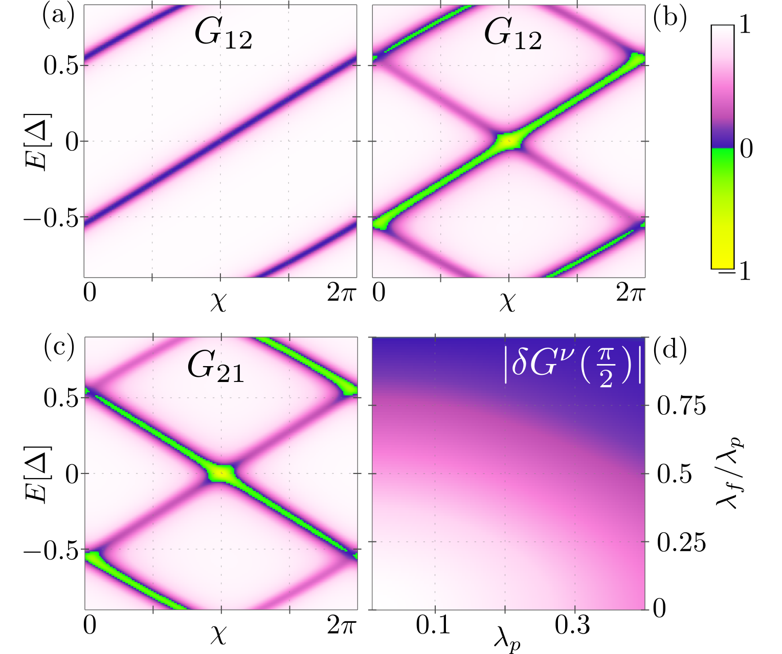
Figure 2: (a-c) Non-local differential conductances $G_{12/21}(E,\chi)$ for the parameters: $\lambda_{p}=0.25$, $\bar{x}=1\xi_{L}$, $\Delta_{L}=\Delta$, $\Delta_{R}=1.2\Delta$, $D=6\xi_{L}$, with the coherence length $\xi_{L}=v/(\pi\Delta_{L})$. In (a) we plot $G_{12}$ for $\lambda_{f}=0$. In (b) and (c) we plot $G_{12}$ and $G_{21}$, respectively, with $\lambda_{f}=0.15$. In (d) we plot $|\delta G^{\nu}|(\pi/2)|$ [see Eq. (8)] as a function of $\lambda_{p}$ and $\lambda_{f}/\lambda_{p}$. All plots share the same color bar, in units of $e^{2}/h$.

If only spin-preserving tunneling is allowed (i.e. $\lambda_{f}=0$), the QPC operates as a perfect spin-resolved Andreev spectrometer: $G_{12}$ ($G_{21}$) is indeed only sensitive to electronic states on the upper edge with spin-up (spin-down). This allows us to perfectly distinguish between the two classes of hABSs, as $G_{12}$ ($G_{21}$) exclusively reveals the energy-phase relation of the $\nu=-1$ ($\nu=+1$) class. In particular, we predict $G_{12}(E,\chi)=G_{21}(E,-\chi)$ with Note that Andreev transmission processes necessarily involve both spin-preserving and spin-flipping tunnelings. Hence, for $\lambda_{f}=0$, we have $c^{he}_{\leftrightarrow}=0$ and $0\leq G_{12/21}\leq e^{2}/h$.

$$G_{12}(E,\chi)=\left[1+\frac{8\lambda_{p}^{4}}{(\lambda_{p}^{4}-1)^{2}(1+\cos(\Phi_{L}+\Phi_{R}-\chi))}\right]^{-1}.$$ (7)

This result is displayed in Fig. 2(a) where, to highlight the robustness of the setup against geometrical asymmetries, we consider a finite $\bar{x}\neq 0$ and $\Delta_{R}\neq\Delta_{L}$ Chang and Bagwell (1994) Since we consider $\Delta_{R}\sim\Delta_{L}$ and finite junction lengths in order to accomodate the QPC (e.g. $D=6\xi_{L}$ in Figs. 2 and 3), we expect to find ABS for all the values of the phase difference $\chi$ Chang and Bagwell (1994).. In this regime, our device can therefore provide a compelling proof of the existence of hABSs and directly probe their particular spin structure.

Importantly, the proposed setup is robust with respect to the two main effects that lead to deviations from the ideal scenario discussed above: (i) Limited spin-resolving power of the detector due to a finite spin-flipping amplitude $\lambda_{f}$ at the QPC; (ii) Presence of spurious reflection mechanisms within the JJ. In the following, we carefully analyze both of them.

Robustness against spin-flip events. — Our device retains a strong spin-sensitivity even in presence of finite $\lambda_{f}$. This is shown, for example, in Figs. 2(b,c), where we plot $G_{12}$ [panel (b)] and $G_{21}$ [panel (c)] for $\lambda_{p}=0.25$ and a relatively large $\lambda_{f}=0.15$. Each conductance is sensitive to both classes of hABSs, since a given spin channel on the lower edge is now coupled to both spin orientations on the upper edge. However, reductions from the quantized value are particularly pronounced only for one of them. The qualitative distinction between the two classes is facilitated by the presence of regions featuring negative values of the conductance, resulting from the onset of the Andreev transmission processes discussed in the next paragraph. To achieve analytical progress, we consider the (reasonable) assumption $\Delta_{R}=\Delta_{L}=\Delta$ that allows us to derive a compact expression for $\delta G^{\nu}(\chi)=G_{12}(E_{\nu},\chi)-G_{21}(E_{\nu},\chi)$,

$$\delta G^{\nu}(\chi)=\frac{e^{2}}{h}\frac{\nu(\lambda_{p}^{2}-\lambda_{f}^{2})(\Lambda^{2}-1)^{2}\sin(\chi)^{2}}{4\Lambda^{3}\cos(\chi)^{2}+\Lambda(\Lambda^{2}+1)^{2}\sin(\chi)^{2}},$$ (8)

with $\Lambda=\lambda_{p}^{2}+\lambda_{f}^{2}$ and $E_{\nu}$ satisfying the energy-phase relations $\Phi(E_{\nu})=(\pi-\nu\chi)/2$ of the hABSs. As expected, the difference vanishes for $\chi=0,\pi$ (when the hABSs are degenerate) and for $\lambda_{p}=\lambda_{f}$ (when the tunneling at the QPC becomes spin-independent). By contrast, the maximum absolute value of $\delta G^{\nu}(\chi)$ is reached for $\chi=\pi/2,3\pi/2$. In Fig. 2(d), we plot $|\delta G^{\nu}(\pi/2)|$ as a function of $\lambda_{p}$ and $\lambda_{f}/\lambda_{p}$ and show that it remains significantly larger than zero even when $\lambda_{f}$ represents a sizable fraction of $\lambda_{p}$. Therefore, even for finite $\lambda_{f}$, the asymmetry between $G_{12}$ and $G_{21}$ remains a good indicator of the existence of two classes of Andreev bound states, with complementary spin-structure and energy-phase relation. Only in the specific case $\lambda_{p}=\lambda_{f}$, tunneling at the QPC becomes completely spin-independent. Then, it is not possible anymore to distinguish between the two hABS classes.

Figs. 2(b,c) show another intriguing feature: When both tunneling amplitudes are finite, it is possible to observe negative values of $G_{12/21}$ (green-yellow regions). Indeed, for $\lambda_{p},\lambda_{f}\neq 0$, Andreev transmission processes $c^{he}_{\leftrightarrow}$ are allowed at the QPC and they can dominate over the standard transmission. This is particularly evident close to the energy-phase relations of the hABSs, where the standard transmission is suppressed. Focusing on $E=0$ and $\chi=\pi$, we find the simple relation $0\geq(G_{12/21}\propto-\lambda_{p}^{2}\lambda_{f}^{2})\geq-{e^{2}/h}$ Sup , stemming from the presence of a Kramers pair of Majorana zero modes (obtained from a proper linear combination of the degenerate hABSs) Li et al. (2016); Pikulin et al. (2016). In general, however, negative values of $G_{12/21}$ can be found at all energies below the gap, and even in absence of hABSs, see Figs. 3(a,b) and Ref. Fleckenstein et al. (2021).

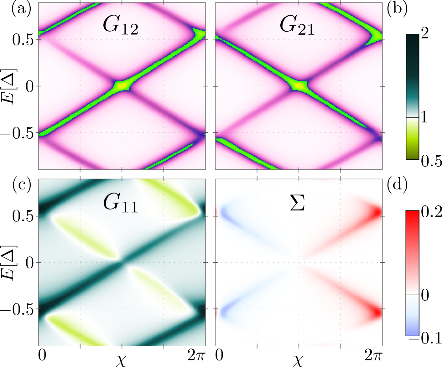
Figure 3: Differential conductances in presence of electronic backscattering on the upper edge, induced by a magnetic impurity with $m=0.05$ and located at $x_{\rm M}=2\xi_{L}$. The other parameters are the same as in Figs.2(b,c). The conductances are in units of $e^{2}/h$. Plots (a,b) share the same color bar with Fig. 2.

Spurious backscattering terms. — To study the effects of spurious backscattering mechanisms within the JJ, we begin by considering the example provided in Figs. 3(a,b). There, we plot the conductances $G_{12/21}$ obtained for the same parameters used in Figs. 2(b,c) but considering the additional presence of a weak magnetic impurity within the JJ. The latter, described by the Hamiltonian $H_{M}=2vm\,\psi_{L\uparrow}^{\dagger}(x_{M})\psi_{R\downarrow}(x_{M})+h.c.$, induces electronic backscattering at $x=x_{\rm M}$ and therefore hybridizes the hABSs. For a small impurity strength $m=0.05\ll 1$, the resulting mid-gap states retain a significant spin-polarization, which emerges as a strong asymmetry between the two non-local conductances in Figs. 3(a,b). While this underlines once more the high spin-sensitivity of our device, a direct comparison with Figs. 2(b,c) shows that a qualitative analysis of $G_{12/21}$ alone might not be able to clearly distinguish between the two cases. In this respect, we stress that a violation of

$$G_{12/21}(E,\chi)=G_{12/21}(-E,-\chi)$$ (9)

represents a proof for the absence of hABSs. However, the converse is not true sup and this calls for a more in-depth analysis of the conductances.

Our device provides us with an additional tool that can efficiently detect the presence of spurious electronic backscattering within the JJ, allowing us to distinguish between the presence of hABSs and other mid-gap states. In particular, our setup naturally allows for the measurement of the local differential conductances

$$\begin{split}G_{11}(V_{1},\chi)&=\frac{dI_{1}}{dV_{1}}=\frac{e^{2}}{h}(1-|r^{ee}_{\hookleftarrow}|^{2}+|a_{\hookleftarrow}^{he}|^{2}),\\ G_{22}(V_{2},\chi)&=\frac{dI_{2}}{dV_{2}}=\frac{e^{2}}{h}(1-|r^{ee}_{\hookrightarrow}|^{2}+|a_{\hookrightarrow}^{he}|^{2}),\end{split}$$ (10)

that can be combined to define

$$\begin{split}\Sigma&=G_{12}+G_{11}-G_{21}-G_{22}\\ &{=2\big{(}|r^{ee}_{\hookrightarrow}|^{2}+|c^{he}_{\leftarrow}|^{2}-|r^{ee}_{\hookleftarrow}|^{2}-|c^{he}_{\rightarrow}|^{2}\big{)}.}\end{split}$$ (11)

The four independent quantities $G_{12/21/11}$ and $\Sigma$ are plotted in Fig. 3. The presence of hABSs implies $\Sigma=0$. Indeed, as each hABS consists only of electrons with a specific spin orientation, there is only one way for electrons to tunnel from (into) that hABS. In particular, the reflection of an electron emerging from contact $C_{j}$ necessarily involves one spin-flipping and one spin-preserving tunneling event, regardless of $j=1,2$. The same applies for the Andreev transmission and leads to $|r^{ee}_{\hookrightarrow}|^{2}=|r^{ee}_{\hookleftarrow}|^{2}$ and $|c^{he}_{\leftarrow}|^{2}=|c^{he}_{\rightarrow}|^{2}$ Sup . By contrast, mid-gap states with non-helical features offer more channels for the electrons to tunnel between the edges. This results in deviations from $\Sigma=0$ as shown in Fig. 3(d). We thus claim that the consistent observation of a vanishing $\Sigma=0$ over a wide range of parameters represents a proof of the presence of hABSs.

To properly demonstrate this, we consider the presence of generic backscattering processes between the two helical channels of the upper edge. To this end, we replace the AR-induced constraints on the scattering amplitudes in Eq. (2) with the more general conditions

$$\begin{pmatrix}\alpha_{r\sigma}^{e}\\ \alpha_{r{\sigma}}^{h}\end{pmatrix}=\begin{pmatrix}\cos(\theta_{r})e^{i\xi^{ee}}_{r}&\sin(\theta_{r})e^{i\xi^{eh}_{r}}\\ \sin(\theta_{r})e^{i\xi^{he}}_{r}&\cos(\theta_{r})e^{i\xi^{hh}_{r}}\\ \end{pmatrix}\begin{pmatrix}\beta_{\tilde{r}\tilde{\sigma}}^{e}\\ \beta_{\tilde{r}\tilde{\sigma}}^{h}\end{pmatrix},$$ (12)

describing generic complete reflection processes happening to the left ($r=L$) or to the right ($r=R$) of the QPC. The parameters $\theta_{r}$ (mod $\pi$) control the nature of these processes, which can continuously range from the pure electronic backscattering limit ($\theta_{r}=0$) to the pure AR scenario considered in Eq. (2) and corresponding to $\theta_{r}=\pi/2$ (with $\xi^{eh/he}_{r}(E)=\mp(\chi_{r}+r\pi/2)+\Phi_{r}(E)$). The analytical expressions of the four differential conductances, determined by imposing Eq. (12), show that the exclusive presence of AR (and thus of hABSs) implies a vanishing $\Sigma=0$ Sup . Moreover, with the possible exception of fine-tuned points in the parameter space, we demonstrate that $\Sigma=0$ also guarantees $\theta_{R}=\theta_{L}=\pi/2$ Strictly speaking, the observation of $\Sigma=0$ implies either $\theta_{R}=\theta_{L}=0$ (i.e. pure electronic backscattering) or $\theta_{R}=\theta_{L}=\pi/2$ (i.e. pure AR). It is however straightforward to distinguish between these to limits. For example, in presence of pure electronic backscattering, no Andreev processes are present and $G_{12/21}$ cannot be negative. Moreover, in this case, the superconductors should not play any role and the conductances are thus expected not to depend on $\chi$., and thus the presence of pure AR Sup . Therefore, the experimental observation of $\Sigma=0$ over a wide range of parameters, e.g. over the $(E-\chi)$ diagram and for different samples featuring different JJ length, QPC transparency and position, represents a proof of the exclusive presence of AR within the JJ. This, in turn, assures that the mid-gap states probed by our spin-resolved Andreev spectrometer are indeed hABSs.

Discussion. — We argue that our proposal is within experimental reach, given the degree of maturity of HgTe-based 2DTI devices. The edge states exhibit ballistic mean free paths that exceed several micrometers Bocquillon et al. (2018); König et al. (2007). We, therefore, expect that inelastic scattering, which would be detrimental both for the formation of hABS and for their detection, should not play a major role in a realization of our proposal based on HgTe. Josephson junctions have been successfully realized, for example with Al contacts, featuring an estimated coherence length $\xi\simeq\,600\,{\rm nm}$ and superconducting gap $\Delta\sim 40\,\mu{\rm eV}$ Bocquillon et al. (2016, 2018). As the physical width of a QPC is typically of the order of $100\,{\rm nm}$ Strunz et al. (2019), the geometrical constraints of our proposal can be satisfied. Importantly, our results are robust with respect to geometrical asymmetries in the setup, as confirmed by Figs. 2 and 3 that have been obtained for an asymmetric position of the QPC and asymmetric pairing potentials $\Delta_{L}\neq\Delta_{R}$.

Appendix A Perfect Andreev reflections

The aim of this section is to derive Eq. (2) of the main text, which describes the phases associated with AR within a JJ. In the setup considered in the main text, the JJ is defined on the upper edge of a 2DTI which has negative helicity, that is $r\sigma=\zeta=-1$. However, for the sake of generality, in the following, we investigate a single helical edge with a generic helicity $\zeta$ (for this reason we can drop the index $r$ of the fermionic fields). Its Hamiltonian reads (in this Section we assume $v=1$)

$$H_{\zeta}=\int dx\sum_{\sigma}\zeta\sigma\psi_{\sigma}^{\dagger}(x)(-i\partial_{x})\psi_{\sigma}(x).$$ (13)

In the portions of the helical system which are proximitized by a standard superconductor, an additional proximity-induced pairing is present

$$H_{\Delta}=\int dx\,\Delta(x)\left[e^{-i\chi}\psi^{\dagger}_{\uparrow}(x)\psi^{\dagger}_{\downarrow}(x)+e^{i\chi}\psi_{\downarrow}(x)\psi_{\uparrow}(x)\right].$$ (14)

The resulting Hamiltonian density in th Bogoliubov-de Gennes (BdG) form reads

$$\mathcal{H}_{\rm BdG}^{\zeta}=\begin{pmatrix}\zeta p&0&0&\Delta(x)e^{-i\chi}\\ 0&-\zeta p&-\Delta(x)e^{-i\chi}&0\\ 0&-\Delta(x)e^{i\chi}&\zeta p&0\\ \Delta(x)e^{i\chi}&0&0&-\zeta p\\ \end{pmatrix}$$ (15)

with $p=-i\partial_{x}$ and written in the basis $\Psi=(\psi_{\uparrow},\psi_{\downarrow},\psi_{\uparrow}^{\dagger},\psi_{\downarrow}^{\dagger})^{T}$.

Focusing on a given proximitized region (and assuming the superconducting pairing to be homogeneous), the BdG equation of the system is given by

$$E\begin{pmatrix}u_{\sigma}\\ v_{\tilde{\sigma}}\end{pmatrix}=\sigma\begin{pmatrix}\zeta p&\Delta e^{-i\chi}\\ \Delta e^{i\chi}&-\zeta p\end{pmatrix}\begin{pmatrix}u_{\sigma}\\ v_{\tilde{\sigma}}\end{pmatrix},$$ (16)

or equivalently

$$-i\partial_{x}\begin{pmatrix}u_{\sigma}\\ -v_{\tilde{\sigma}}\end{pmatrix}=\zeta\begin{pmatrix}\sigma E&\Delta e^{-i\chi}\\ -\Delta e^{i\chi}&-\sigma E\end{pmatrix}\begin{pmatrix}u_{\sigma}\\ -v_{\tilde{\sigma}}\end{pmatrix},$$ (17)

where we denote the eigenvectors of $\mathcal{H}_{\rm BdG}^{\zeta}$, with eigenvalue $E$, as $\phi=(u_{\uparrow},u_{\downarrow},v_{\uparrow},v_{\downarrow})^{T}$. Its solutions read

$$\begin{pmatrix}u_{\sigma}\\ v_{\tilde{\sigma}}\end{pmatrix}=A_{+}e^{\kappa x}\begin{pmatrix}e^{-i\chi}(\zeta\sigma E-i\kappa)\\ \zeta\Delta\end{pmatrix}+A_{-}e^{-\kappa x}\begin{pmatrix}e^{-i\chi}(\zeta\sigma E+i\kappa)\\ \zeta\Delta\end{pmatrix},$$ (18)

where we introduce $\kappa=\sqrt{\Delta^{2}-E^{2}}$. By contrast, in the non-proximitized helical region, we have $\Delta=0$ and the solutions of the BdG equations are simply plane waves

$$\begin{pmatrix}u_{\sigma}\\ v_{\tilde{\sigma}}\end{pmatrix}=\begin{pmatrix}Ae^{i\zeta\sigma Ex}\\ Be^{-i\zeta\sigma Ex}\end{pmatrix}=\begin{pmatrix}Ae^{-i\zeta\tilde{\sigma}Ex}\\ Be^{i\zeta\tilde{\sigma}Ex}\end{pmatrix}.$$ (19)

Let us now consider the reflections from two semi-infinite superconductors located at $x=x_{r}$, with $r=R,L$. At first, we focus on an incident electronic plane wave with energy $E$ and amplitude $\beta_{r\sigma}^{e}$ [see Fig. 1(c) of the main text for a sketch of our notation]. The Andreev reflected hole has an amplitude given by the solution of

$$\begin{cases}\beta_{r\sigma}^{e}e^{irEx_{r}}=Ce^{-i\chi_{r}}(rE+ri\kappa_{r})\\ \alpha_{\tilde{r}\tilde{\sigma}}^{h}e^{-irEx_{r}}=Cr\sigma\Delta_{r}\end{cases}$$ (20)

which gives us

$$\alpha_{\tilde{r}\tilde{\sigma}}^{h}=e^{i2rEx_{r}}e^{i\chi_{r}}\frac{\sigma\Delta_{r}}{E+i\kappa_{r}}\beta_{r\sigma}^{e}=\sigma e^{i2rEx_{r}}e^{i\chi_{r}}e^{-i\arccos(E/\Delta_{r})}\beta_{r\sigma}^{e}.$$ (21)

As for the scattering of holes with energy $E$ and amplitude $\beta_{\tilde{r}\tilde{\sigma}}^{h}$, we get

$$\begin{cases}\alpha_{\tilde{r}\tilde{\sigma}}^{e}e^{-irEx_{r}}=Ce^{-i\chi_{r}}(-rE+ri\kappa_{r})\\ \beta_{r\sigma}^{h}e^{irEx_{r}}=-Cr\tilde{\sigma}\Delta_{r}\end{cases}$$ (22)

which results in

$$\alpha_{\tilde{r}\tilde{\sigma}}^{e}=e^{i2rEx_{r}}e^{-i\chi_{r}}\frac{E-i\kappa_{r}}{\tilde{\sigma}\Delta_{r}}\beta_{r\sigma}^{h}=\tilde{\sigma}e^{i2rEx_{r}}e^{-i\chi_{r}}e^{-i\arccos(E/\Delta_{r})}\beta_{r\sigma}^{h}.$$ (23)

Note that we use the identity ($|E|<\Delta$)

$$\frac{\Delta}{E+i\sqrt{\Delta^{2}-E^{2}}}=\exp\left[-i\arccos\frac{\Delta}{E}\right].$$ (24)

In summary, we obtain ($c=e/h=\pm 1$, $\tilde{e}=h$)

$${\alpha_{r\sigma}^{c}=c\sigma\exp\left[-ic\chi_{\tilde{r}}+2\tilde{r}iEx_{\tilde{r}}-i\arccos(E/\Delta_{\tilde{r}})\right]\beta_{\tilde{r}\tilde{\sigma}}^{\tilde{c}}}.$$ (25)

The parameters $\chi_{r}$ and $\Delta_{r}$ are the superconducting phase and pairing potential of the right ($r=R$) and left ($r=L$) superconducting lead. Note that, if the two superconductors are located at $x_{r}=rD/2$, one simply gets $2\tilde{r}iEx_{\tilde{r}}=iED$ regardless of the value of $r$. Eq. (25) demonstrates the validity of Eq. (2) of the main text.

Incidentally, we observe that Eq. (25) is compatible with particle-hole symmetry. The latter exchanges particles and holes $\alpha^{c}_{r\sigma}\to\alpha^{\tilde{c}}_{r\sigma}$ and $\beta^{c}_{r\sigma}\to\beta^{\tilde{c}}_{r\sigma}$, adds a complex conjugation $i\to-i$, and flips the sign of the energy $E\to-E$. It is easy to verify that (25) is invariant under particle-hole symmetry

$$\begin{split}&\alpha_{r\sigma}^{c}=c\sigma\exp\left[-ic\chi_{\tilde{r}}+2\tilde{r}iEx_{\tilde{r}}\right]\frac{\Delta_{\tilde{r}}}{E+i\kappa_{\tilde{r}}}\beta_{\tilde{r}\tilde{\sigma}}^{\tilde{c}}\quad\overset{\tiny{P.H.}}{\Rightarrow}\quad\alpha_{r\sigma}^{\tilde{c}}=-c\sigma\exp\left[+ic\chi_{\tilde{r}}+2\tilde{r}iEx_{\tilde{r}}\right]\frac{\Delta_{\tilde{r}}}{E+i\kappa_{\tilde{r}}}\beta_{\tilde{r}\tilde{\sigma}}^{c}\end{split}$$ (26)

As for time-reversal symmetry, it add a complex conjugation $i\to-i$, exchanges incoming and outgoing states, flips the propagation direction and the spin, and add a spin-dependent sign to the amplitudes, i.e. $\alpha^{c}_{r\sigma}\to\sigma\beta^{c}_{\tilde{r}\tilde{\sigma}}$ and $\beta^{c}_{r\sigma}\to\sigma\alpha^{c}_{\tilde{r}\tilde{\sigma}}$. Eq. (25) is not invariant under time-reversal symmetry, since the latter flips the sign of the superconducting phases. In particular, one obtains

$$\begin{split}&\alpha_{r\sigma}^{c}=c\sigma\exp\left[-ic\chi_{\tilde{r}}+2\tilde{r}iEx_{\tilde{r}}\right]\frac{\Delta_{\tilde{r}}}{E+i\kappa_{\tilde{r}}}\beta_{\tilde{r}\tilde{\sigma}}^{\tilde{c}}\quad\overset{\tiny{T.R.}}{\Rightarrow}\quad\alpha_{r\sigma}^{c}=c\sigma\exp\left[+ic\chi_{\tilde{r}}+2\tilde{r}iEx_{\tilde{r}}\right]\frac{\Delta_{\tilde{r}}}{E+i\kappa_{\tilde{r}}}\beta_{\tilde{r}\tilde{\sigma}}^{\tilde{c}}.\end{split}$$ (27)

Appendix B Scattering matrix of the QPC

The goal of this section is to derive the scattering matrix of the QPC, both for electron ($S^{e}_{\rm QPC}$) and hole ($S^{h}_{\rm QPC}$) states, starting from the Hamiltonian $H_{0}$ of the helical edges [see Eq. (1) of the main text] and from the one describing tunneling at the QPC $H_{\rm QPC}$ [see Eq. (4) of the main text] located at $x=\bar{x}$. We remind the reader that, in order for the QPC to be time-reversal invariant, we consider real amplitudes for both spin-preserving ($\lambda_{p}$) and spin-flipping ($\lambda_{f}$) tunneling amplitudes. It is straightforward to compute the equations of motion of the field operators, i.e. $i\partial_{t}\psi_{r\sigma}=-[H_{0}+H_{\rm QPC},\psi_{r\sigma}]$, that give

$$i\partial_{t}\psi_{r\sigma}=-i\vartheta_{r}v\partial_{x}\psi_{r\sigma}+2v\delta(x-\bar{x})\left(\lambda_{p}\psi_{\tilde{r}\sigma}+\vartheta_{r}\lambda_{f}\psi_{r\tilde{\sigma}}\right)$$ (28)

where $\tilde{\uparrow}=\downarrow$, $\tilde{R}=L$ and vice-versa. By using the plane-wave ansatz

$$\psi_{r\sigma}(x)=\frac{e^{-iEt}}{\sqrt{\hbar v}}\begin{cases}\alpha_{r\sigma}e^{irEx/v}\qquad&r(x-\bar{x})<0\\ \beta_{r\sigma}e^{irEx/v}\qquad&r(x-\bar{x})>0\end{cases},$$ (29)

we can relate incoming and outgoing amplitudes as

$$i(\beta_{r\sigma}-\alpha_{r\sigma})=\lambda_{p}e^{-2\vartheta_{r}iE\bar{x}/v}(\beta_{\tilde{r}\sigma}+\alpha_{\tilde{r}\sigma})+\vartheta_{r}\lambda_{f}(\beta_{r\tilde{\sigma}}+\alpha_{r\tilde{\sigma}}).$$ (30)

By rearranging terms, we get

$$\begin{split}&\begin{pmatrix}i&\lambda_{f}&-\lambda_{p}e^{2iE\bar{x}/v}&\\ \lambda_{f}&i&&-\lambda_{p}e^{2iE\bar{x}/v}\\ -\lambda_{p}e^{-2iE\bar{x}/v}&&i&-\lambda_{f}\\ &-\lambda_{p}e^{-2iE\bar{x}/v}&-\lambda_{f}&i\\ \end{pmatrix}\begin{pmatrix}\beta_{L\uparrow}\\ \beta_{L\downarrow}\\ \beta_{R\uparrow}\\ \beta_{R\downarrow}\end{pmatrix}=\\ &\qquad\begin{pmatrix}i&-\lambda_{f}&\lambda_{p}e^{2iE\bar{x}/v}&\\ -\lambda_{f}&i&&\lambda_{p}e^{2iE\bar{x}/v}\\ \lambda_{p}e^{-2iE\bar{x}/v}&&i&\lambda_{f}\\ &\lambda_{p}e^{-2iE\bar{x}/v}&\lambda_{f}&i\\ \end{pmatrix}\begin{pmatrix}\alpha_{L\uparrow}\\ \alpha_{L\downarrow}\\ \alpha_{R\uparrow}\\ \alpha_{R\downarrow}\end{pmatrix},\end{split}$$ (31)

which allows us to readily derive the electronic scattering matrix $S^{e}_{\rm QPC}$ as

$$\begin{pmatrix}\beta^{e}_{L\uparrow}\\ \beta^{e}_{L\downarrow}\\ \beta^{e}_{R\uparrow}\\ \beta^{e}_{R\downarrow}\end{pmatrix}=\begin{pmatrix}\Lambda_{pf}&\Lambda_{ff}&\Lambda_{pb}&0\\ \Lambda_{ff}&\Lambda_{pf}&0&\Lambda_{pb}\\ -\Lambda_{pb}^{*}&0&\Lambda_{pf}&-\Lambda_{ff}\\ 0&-\Lambda_{pb}^{*}&-\Lambda_{ff}&\Lambda_{pf}\\ \end{pmatrix}\begin{pmatrix}\alpha^{e}_{L\uparrow}\\ \alpha^{e}_{L\downarrow}\\ \alpha^{e}_{R\uparrow}\\ \alpha^{e}_{R\downarrow}\end{pmatrix}$$ (32)

with

$$\Lambda_{pf} =\frac{1-\lambda_{f}^{2}-\lambda_{p}^{2}}{1+\lambda_{f}^{2}+\lambda_{p}^{2}},$$ (33)

$$\Lambda_{ff} =\frac{2i\lambda_{f}}{1+\lambda_{f}^{2}+\lambda_{p}^{2}},$$ (34)

$$\Lambda_{pb} =-\frac{2i\lambda_{p}e^{2iE\bar{x}/v}}{1+\lambda_{f}^{2}+\lambda_{p}^{2}}.$$ (35)

In presence of superconductivity, it is convenient to compute the scattering matrix also for incoming and outgoing holes. In this case, the amplitudes $\alpha^{h}_{r\sigma}$ and $\beta^{h}_{r\sigma}$ are related by the scattering matrix $S^{h}(\lambda_{p},\lambda_{f})=S^{e}(-\lambda_{p},-\lambda_{f})$, i.e.

$$\begin{pmatrix}\beta^{h}_{L\uparrow}\\ \beta^{h}_{L\downarrow}\\ \beta^{h}_{R\uparrow}\\ \beta^{h}_{R\downarrow}\end{pmatrix}=\begin{pmatrix}\Lambda_{pf}&-\Lambda_{ff}&-\Lambda_{pb}&0\\ -\Lambda_{ff}&\Lambda_{pf}&0&-\Lambda_{pb}\\ \Lambda_{pb}^{*}&0&\Lambda_{pf}&\Lambda_{ff}\\ 0&\Lambda_{pb}^{*}&\Lambda_{ff}&\Lambda_{pf}\\ \end{pmatrix}\begin{pmatrix}\alpha^{h}_{L\uparrow}\\ \alpha^{h}_{L\downarrow}\\ \alpha^{h}_{R\uparrow}\\ \alpha^{h}_{R\downarrow}\end{pmatrix}.$$ (36)

Appendix C Scattering matrix on the lower edge

In this section, we combine the perfect AR on the upper edge with the scattering at the QPC, aiming at deriving the scattering matrix for the amplitudes on the lower helical edge. By solving the resulting linear system for $\beta^{e}_{R\uparrow},\beta^{e}_{L\downarrow},\beta^{h}_{R\uparrow}$, and $\beta^{h}_{L\downarrow}$ we readily obtain Eq. (5) of the main text. The latter reads

$$\begin{pmatrix}\beta_{R}^{e}\\ \beta_{L}^{e}\\ \beta_{R}^{h}\\ \beta_{L}^{h}\end{pmatrix}=\begin{pmatrix}t^{ee}_{\rightarrow}&r^{ee}_{\hookrightarrow}&c^{eh}_{\rightarrow}&a^{eh}_{\hookrightarrow}\\ r^{ee}_{\hookleftarrow}&t^{ee}_{\leftarrow}&a^{eh}_{\hookleftarrow}&c^{eh}_{\leftarrow}\\ c^{he}_{\rightarrow}&a^{he}_{\hookrightarrow}&t^{hh}_{\rightarrow}&r^{hh}_{\hookrightarrow}\\ a^{he}_{\hookleftarrow}&c^{he}_{\leftarrow}&r^{hh}_{\hookleftarrow}&t^{hh}_{\leftarrow}\end{pmatrix}\begin{pmatrix}\alpha_{R}^{e}\\ \alpha_{L}^{e}\\ \alpha_{R}^{h}\\ \alpha_{L}^{h}\end{pmatrix}$$ (37)

where we suppressed the redundant spin index, which is fixed by the (positive) helicity of the lower helical edge.

It is interesting to show and comment on the analytical expression of the transmission and reflections coefficients. To this end, it is particularly convenient to use the functions $\Phi_{r}(E)$ functions defined in the main text. The coefficients associated with an incoming electron with spin-up (i.e. from the $C_{1}$ lead) reads

$$t^{ee}_{\rightarrow} =\frac{(\lambda_{p}^{2}+\lambda_{f}^{2})^{2}-1}{\Omega}\Big{[}e^{i(\chi+2\Phi_{R}+2\Phi_{L})}(\lambda_{p}^{2}+\lambda_{p}^{2}-1)^{2}+e^{i\chi}(\lambda_{p}^{2}+\lambda_{p}^{2}+1)^{2}$$ (38)

$$\qquad+e^{i(\Phi_{L}+\Phi_{R}+2\chi)}(\lambda_{p}^{4}+2\lambda_{p}^{2}(\lambda_{f}^{2}-1)+(1+\lambda_{f}^{2})^{2})+e^{i(\Phi_{L}+\Phi_{R})}(\lambda_{f}^{4}+2\lambda_{f}^{2}(\lambda_{p}^{2}-1)+(1+\lambda_{p}^{2})^{2})\Big{]}$$

$$r^{ee}_{\hookleftarrow} =\frac{4e^{2iE\bar{x}/v}}{\Omega}e^{i(\Phi_{L}+\Phi_{R})}(e^{2i\chi}-1)\lambda_{f}\lambda_{p}((\lambda_{p}^{2}+\lambda_{f}^{2})^{2}-1)$$ (39)

$$c^{he}_{\rightarrow} =\frac{8\lambda_{f}\lambda_{p}e^{i\chi}}{\Omega}\Big{[}(\lambda_{p}^{2}+\lambda_{f}^{2}-1)^{2}e^{i3(\Phi_{L}+\Phi_{R})/2}\sin\tfrac{4E\bar{x}/v+\chi+\Phi_{L}-\Phi_{R}}{2}+(\lambda_{p}^{2}+\lambda_{f}^{2}+1)^{2}e^{i(\Phi_{L}+\Phi_{R})/2}\sin\tfrac{4E\bar{x}/v+\Phi_{L}-\Phi_{R}-\chi}{2}\Big{]}$$ (40)

$$a^{he}_{\hookleftarrow} =-\frac{4ie^{i\chi/2}}{\Omega}\Big{[}\lambda_{f}^{2}(\lambda_{p}^{2}+\lambda_{f}^{2}-1)^{2}e^{i(\Phi_{L}+2\Phi_{R})}+\lambda_{p}^{2}(\lambda_{p}^{2}+\lambda_{f}^{2}-1)^{2}e^{i(4E\bar{x}/v+2\Phi_{L}+\Phi_{R}+\chi)}$$ (41)

$$\qquad+\lambda_{f}^{2}(\lambda_{p}^{2}+\lambda_{f}^{2}+1)^{2}e^{i(\Phi_{R}+\chi)}+\lambda_{p}^{2}(\lambda_{p}^{2}+\lambda_{f}^{2}+1)^{2}e^{i(\Phi_{L}+4E\bar{x}/v)}\Big{]}$$

with the denominator

$$\Omega=\Big{[}(\lambda_{p}^{2}+\lambda_{f}^{2}+1)^{2}+(\lambda_{p}^{2}+\lambda_{f}^{2}-1)^{2}e^{i(\Phi_{L}+\Phi_{R}+\chi)}\Big{]}\Big{[}(\lambda_{p}^{2}+\lambda_{f}^{2}+1)^{2}e^{i\chi}+(\lambda_{p}^{2}+\lambda_{f}^{2}-1)^{2}e^{i(\Phi_{L}+\Phi_{R})}\Big{]}.$$ (42)

The other coefficients of the scattering matrix are given by

$$t^{hh/ee}_{\leftarrow} =t^{ee/hh}_{\rightarrow}$$ (43)

$$t^{ee}_{\leftarrow}(\lambda_{p},\lambda_{f}) =t^{ee}_{\rightarrow}(\lambda_{f},\lambda_{p})$$ (44)

$$r^{hh}_{\hookleftarrow} =-r^{ee}_{\hookleftarrow}$$ (45)

$$r^{hh}_{\hookrightarrow} =-r^{ee}_{\hookrightarrow}=-e^{-4iE\bar{x}/v}r^{ee}_{\hookleftarrow}$$ (46)

$$c^{he/eh}_{\leftarrow} =-c^{he/eh}_{\rightarrow}$$ (47)

$$c^{eh}_{\rightarrow}(-\chi) =-e^{-2i\chi}c^{he}_{\rightarrow}(\chi)$$ (48)

$$a^{eh}_{\hookleftarrow}(-\chi) =-e^{-2i\chi}a^{he}_{\hookleftarrow}(\chi)$$ (49)

$$a^{eh}_{\hookrightarrow}(-\chi) =-e^{-2i\chi}a^{he}_{\hookrightarrow}(\chi)$$ (50)

$$a^{he}_{\hookrightarrow}(\lambda_{p},\lambda_{f}) =-e^{-4iE\bar{x}/v}a^{he}_{\hookleftarrow}(\lambda_{f},\lambda_{p}).$$ (51)

Note that the modulus squared of the standard transmission and reflection coefficients does not depend on the position $\bar{x}$ of the QPC. By contrast, the Andreev transmission and reflection coefficients do depend on $\bar{x}$ at finite energy. We also point out that Andreev transmission $c$ and standard reflection $r$ are both proportional to $\lambda_{p}\lambda_{f}$: Those processes are therefore present only when both spin-preserving and spin-flipping tunneling events are allowed. As expected, the standard reflections vanish for $\chi=0,\pi$, i.e. when the whole system is time-reversal symmetric and backscattering within a single helical edge is therefore forbidden.

C.1 Particular values of phase and energy

We observe that the standard transmission coefficient vanishes for $\chi=\pi$ and $E=0$ (which implies $\Phi_{L}=\Phi_{R}=0$) that is, when the JJ host a Kramers pair of Majorana zero modes and only Andreev processes are allowed. In this case, the other coefficients reads

$$r^{ee}_{\hookleftarrow} =0$$ (52)

$$c^{he}_{\rightarrow} =\frac{-2\lambda_{f}\lambda_{p}}{\lambda_{f}^{2}+\lambda_{p}^{2}}$$ (53)

$$a^{he}_{\hookleftarrow} =\frac{\lambda_{f}^{2}-\lambda_{p}^{2}}{\lambda_{f}^{2}+\lambda_{p}^{2}},$$ (54)

which lead to $G_{12}(0,\pi)=G_{21}(0,\pi)=-(e^{2}/h)\,{4\lambda_{f}^{2}\lambda_{p}^{2}}/{(\lambda_{f}^{2}+\lambda_{p}^{2})^{2}}$. As stated in the main text, we thus have $-e^{2}/h\leq G_{12}(0,\pi)=G_{21}(0,\pi)\leq 0$ and the value of $-e^{2}/h$ is reached for $\lambda_{p}=\lambda_{f}$.

It is illustrative to consider the case $\Delta_{R}=\Delta_{L}$, which leads to $\Phi_{L}=\Phi_{R}=\Phi$. In this case, given the general relation in Eq. (3) of the main text, the energy-phase relation for the $\nu$ class of ABSs is simply given by

$$\Phi^{\nu}(\chi)=(\pi-\nu\chi)/2.$$ (55)

By plugging this relation into the expressions of the coefficients, the latter greatly simplify. This allows us to obtain more concise expressions for the conductances. In particular, if we consider the difference between the two non-local conductances $G_{12}$ and $G_{21}$, computed for the same $\chi$ and for the same energy $E$ which satisfy $\Phi(E)=\Phi^{\nu}(\chi)$, we get

$$\delta G(\chi,\nu)=\nu\frac{e^{2}}{h}\frac{(\lambda_{p}^{2}-\lambda_{f}^{2})((\lambda_{p}^{2}+\lambda_{f}^{2})^{2}-1)^{2}\sin(\chi)^{2}}{4(\lambda_{f}^{2}+\lambda_{p}^{2})^{3}\cos(\chi)^{2}+(\lambda_{p}^{2}+\lambda_{f}^{2})((\lambda_{p}^{2}+\lambda_{f}^{2})^{2}-1)^{2}\sin(\chi)^{2}}.$$ (56)

Such an expression vanishes for $\chi=0,\pi$, i.e. when ABSs belonging to different classes are present at the same time, and reaches its largest absolute value for $\chi=\pm\pi/2$. For $\chi=\pi/2$ and $\nu=+1$, we obtain the expression reported in Eq. (8) of the main text.

Appendix D Spurious backscattering on the upper edge

By combining the scattering at the QPC, described in Eqs. (32) and (36), with the generic reflection matrix in Eq. (11) of the main text, it is straightforward to compute the coefficients of the resulting scattering matrix on the lower edge (whose structure is shown in Eq. (5) of the main text). The analytical expressions of those coefficients, which allow us to compute the conductances discussed in the main text, are extremely lengthy and it is not convenient to explicitly write them here. It is, however, extremely useful to consider particular combinations of those coefficients, such as the quantity $\Sigma$ defined in Eq. (10) of the main text. Since the scattering matrix is unitary, the modulus squared of the coefficients of Andreev reflections ($|a^{he}|$) can be expressed in terms of the others. This allows us to write

$$\begin{split}\Sigma&=G_{12}+G_{11}-G_{21}-G_{22}\\ &=(|t^{ee}_{\rightarrow}|^{2}-|c^{he}_{\rightarrow}|^{2})-(|t^{ee}_{\leftarrow}|^{2}-|c^{he}_{\leftarrow}|^{2})+(1-|r^{ee}_{\hookleftarrow}|^{2}+|a^{he}_{\hookleftarrow}|^{2})-(1-|r^{ee}_{\hookrightarrow}|^{2}+|a^{he}_{\hookrightarrow}|^{2})\\ &=(|t^{ee}_{\rightarrow}|^{2}-|c^{he}_{\rightarrow}|^{2})-(|t^{ee}_{\leftarrow}|^{2}-|c^{he}_{\leftarrow}|^{2})+(2-2|r^{ee}_{\hookleftarrow}|^{2}-|t^{ee}_{\rightarrow}|^{2}-|c^{he}_{\rightarrow}|^{2})-(2-2|r^{ee}_{\hookrightarrow}|^{2}-|t^{ee}_{\leftarrow}|^{2}-|c^{he}_{\leftarrow}|^{2})\\ &=2\left[|r^{ee}_{\hookrightarrow}|^{2}+|c^{he}_{\leftarrow}|^{2}-|r^{ee}_{\hookleftarrow}|^{2}-|c^{he}_{\rightarrow}|^{2}\right].\end{split}$$ (57)

Given Eqs. (46) and (47), it is straightforward to show that the presence of hABSs necessarily leads to $|r^{ee}_{\hookrightarrow}|^{2}=|r^{ee}_{\hookleftarrow}|^{2}$ and $|c^{he}_{\leftarrow}|^{2}=|c^{he}_{\rightarrow}|^{2}$, and thus to $\Sigma=0$. Importantly, in the main text we claim that $\Sigma=0$ also implies the existence of hABSs. Before giving a more mathematical proof of this statement, we discuss the physical picture behind it.

D.1 Physical intuition

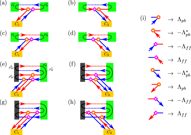
Figure 4: Sketch of the processes that contribute to the reflection at the QPC of electrons on the lower edge. As in Fig. 1 of the main text, blue (red) lines indicate spin-up (spin-down) channels, while solid (dotted) line indicate electron (hole) channels. Moreover, green (yellow) rectangles indicate superconducting (normal) electrodes. Spin-preserving (spin-flipping) tunneling events at the QPC are denoted by orange circles (pink diamonds). In (a-d) we consider the presence of a single hABS with $\nu=-1$, i.e. consisting of left-moving spin-up electrons and right-moving spin-down holes. In (e-h) we consider a bound state resulting from the presence of a strong magnetic region (dark gray) to the left of the QPC, which induces perfect electronic backscattering. In (i), according to Eq. (32), we show the amplitudes associated with each tunneling event.

Let us carefully analyze the reflection coefficients for electrons emerging from the contacts $C_{1}$ and $C_{2}$, i.e. $r_{\hookleftarrow}^{ee}$ and $r_{\hookrightarrow}^{ee}$. In particular, we want to highlight the differences between two scenarios. In case (I), we consider the presence of hABSs on the upper edge. In case (II), we consider the existence of a completely different mid-gap state on the upper edge, resulting from the presence of perfect electronic backscattering to the left of the QPC. Case (II) could stem from the presence of a magnetic barrier placed to the left of the QPC or, equivalently, to a point-like magnetic impurity, described by the Hamiltonian $H_{M}$ in the main text, in the limit $m=1$ (see Sec. E for more details).

These two cases allow us to show how the nature of the bound state located on the upper edge has a direct effect on the possible paths that an incoming electron, from the lower edge, can follow before being eventually reflected back. Those paths are sketched in Fig. 4, where spin-preserving and spin-flipping tunnelings at the QPC are highlighted with orange circles and pink diamonds, respectively. The corresponding amplitudes, according to Eq. (32), are summarized for clarity in Fig. 4(i). Unitary reflections happening at the interfaces with superconductors (in green) are depicted with curved lines and associated with the complex phases $\rho^{\pm}_{L/R}$. Analogously, unitary reflections at the interface with the magnetic barrier (in gray) are associated with the complex phases $\rho_{M}^{e/h}$. Note that spin-preserving forward-scattering events at the QPC (associated with the amplitude $\Lambda_{pf}$ in Eq. (32)) are not explicitly shown. The reflection coefficients $r_{\hookleftarrow}^{ee}$ and $r_{\hookrightarrow}^{ee}$ can be calculated by summing all the amplitudes associated with the allowed paths.

Let us focus on case (I), sketched in Fig. 4(a-d). A spin-up electron impinging on the QPC from contact $C_{1}$ can tunnel to the upper edge either via a spin-flipping [panel (a)] or spin-preserving [panel (c)] tunneling event, coupling to one of the two different classes of hABSs with $\nu=+1$ and $\nu=-1$. However, the only way for this electron to be reflected to contact $C_{1}$ is to tunnel back into the lower edge with via a tunneling event of opposite nature. The whole reflection process, therefore, necessarily consists of both a spin-preserving and a spin-flipping tunneling event at the QPC. By summing over all the possible paths, we can express the reflection amplitude as

$$\begin{split}r_{\hookleftarrow}^{ee}&=-\sum_{\nu=\pm}\nu\Lambda_{pb}\Lambda_{pf}\Lambda_{ff}\,\rho_{L}^{\nu}\rho_{R}^{\nu}\,\sum_{k=0}^{\infty}(\rho_{L}^{\nu}\rho_{R}^{\nu}\Lambda_{pf}^{2})^{k}\\ &=-\Lambda_{pb}\Lambda_{pf}\Lambda_{ff}\sum_{\nu=\pm}\frac{\nu\rho_{L}^{\nu}\rho_{R}^{\nu}}{1-\rho_{L}^{\nu}\rho_{R}^{\nu}\Lambda_{pf}^{2}},\end{split}$$ (58)

where we take into account the possibility of $k$ additional reflections between the two superconductors on the upper edge. As for spin-down electrons coming from contact $C_{2}$, the case depicted in Fig. 4(b,d), we obtain

$$\begin{split}r_{\hookrightarrow}^{ee}&=+\Lambda_{pb}^{*}\Lambda_{pf}\Lambda_{ff}\sum_{\nu=\pm}\frac{\nu\rho_{L}^{\nu}\rho_{R}^{\nu}}{1-\rho_{L}^{\nu}\rho_{R}^{\nu}\Lambda_{pf}^{2}}\end{split}$$ (59)

These expressions, which are compatible with Eqs. (39) and (46), merely differ by a global phase and they clearly satisfy $|r_{\hookleftarrow}^{ee}|^{2}=|r_{\hookrightarrow}^{ee}|^{2}$.

The scattering processes are distinctively different in case (II), displayed in Fig. 4(e-h). Again, a spin-up electron coming from the contact $C_{1}$ can tunnel to the upper edge both via a spin-preserving [panel (e)] and via a spin-flipping tunneling event [panel (g)]. However, regardless of the nature of this first tunneling event, the electron can tunnel back to the lower edge and reach contact $C_{1}$ in two different ways, i.e. by preserving of flipping its spin. As a result, there are four different kinds of paths that contribute to $r_{\hookleftarrow}^{ee}$. Their sum reads

$$\begin{split}r_{\hookleftarrow}^{ee}&=\frac{1}{1-\rho_{M}^{e}\rho_{R}^{+}\rho_{M}^{h}\rho_{R}^{-}\Lambda_{pf}^{4}}\Big{[}\Lambda_{pb}\rho_{M}^{e}\Lambda_{pb}+\Lambda_{pb}\rho_{M}^{e}\rho_{R}^{+}\rho_{M}^{h}\rho_{R}^{-}\Lambda_{pf}^{3}\Lambda_{ff}-\Lambda_{ff}\rho_{R}^{+}\rho_{M}^{h}\rho_{R}^{-}\Lambda_{pf}^{2}\Lambda_{ff}-\Lambda_{ff}\rho_{M}^{e}\rho_{R}^{+}\rho_{M}^{h}\rho_{R}^{-}\Lambda_{pf}^{3}\Lambda_{pb}\Big{]}\\ &=\frac{1}{1-\rho_{M}^{e}\rho_{R}^{+}\rho_{M}^{h}\rho_{R}^{-}\Lambda_{pf}^{4}}\Big{[}\Lambda_{pb}^{2}\rho_{M}^{e}-\Lambda_{ff}^{2}\Lambda_{pf}^{2}\rho_{R}^{+}\rho_{M}^{h}\rho_{R}^{-}\Big{]}.\end{split}$$ (60)

As for spin-down electrons coming from contact $C_{2}$, by looking at Fig. 4(f,h), we get

$$\begin{split}r_{\hookrightarrow}^{ee}&=\frac{1}{1-\rho_{M}^{e}\rho_{R}^{+}\rho_{M}^{h}\rho_{R}^{-}\Lambda_{pf}^{4}}\Big{[}(\Lambda_{pb}^{*})^{2}\Lambda_{pf}^{2}\rho_{R}^{+}\rho_{M}^{h}\rho_{R}^{-}-\Lambda_{ff}^{2}\rho_{M}^{e}\Big{]}.\end{split}$$ (61)

Those two terms differ more than just for a global phase factor, leading to $|r_{\hookleftarrow}^{ee}|^{2}\neq|r_{\hookrightarrow}^{ee}|^{2}$. The same argument applies to the Andreev transmission coefficients. Hence, a mid-gap state consisting of electronic channels with both spin orientations (i.e. not an hABS), which we mimic in our model by the presence of a magnetic scatterer, results in $\Sigma\neq 0$.

D.2 General proof

In the following, under general assumptions, we demonstrate that $\Sigma=0$ implies $\theta_{r}=0,\pi/2$ (mod $\pi$), thus proving the existence of hABSs. To this end, we analytically compute $\Sigma$ as a function of all the parameters of the systems with the generic reflection matrices [see Eq. (11) of the main text], i.e.

$$\Sigma(\lambda_{p},\lambda_{f},E,\bar{x},\theta_{L},\xi^{ee}_{L},\xi^{eh}_{L},\xi^{he}_{L},\xi^{hh}_{L},\theta_{R},\xi^{ee}_{R},\xi^{eh}_{R},\xi^{he}_{R},\xi^{hh}_{R})=\frac{\mathcal{N}}{\mathcal{D}}.$$ (62)

The denominator $\mathcal{D}$ is a bounded function and the numerator $\mathcal{N}$ is a polynomial in $\lambda_{p}$ and $\lambda_{f}$. Requiring that $\Sigma=0$ regardless of the specific value of the tunneling amplitudes at the QPC is equivalent to require that each coefficient $\mathcal{C}_{n,m}$ that multiplies $\lambda_{p}^{n}\lambda_{f}^{m}$ in $\mathcal{N}$ vanishes. Among the several resulting conditions that have to be met, we focus on one of them, $\mathcal{C}_{2,6}+2\mathcal{C}_{4,6}=0$, which can be conveniently expressed as

$$f(\bar{x},E,\eta_{L},\eta_{R})+f(-\bar{x},E,\eta_{R},\eta_{L})=0,$$ (63)

with

$$\begin{split}f(\bar{x},E,\eta_{L},\eta_{R})&=\cos(\theta_{L})\sin(\theta_{R})\Big{[}2\sin(\theta_{L})(\cos(2E\bar{x}+\xi^{ee}_{L}-\xi^{eh}_{L}-\xi^{he}_{R})-\cos(2E\bar{x}+\xi^{ee}_{L}-\xi^{eh}_{R}-\xi^{he}_{L})\\ &\qquad+\cos(2E\bar{x}-\xi^{ee}_{L}+\xi^{he}_{L}-\xi^{he}_{R})+\cos(2Ex+\xi^{he}_{L}-\xi^{he}_{R}-\xi^{hh}_{L}))\\ &\qquad+2\sin(\theta_{R})(\cos(2E\bar{x}+\xi^{ee}_{L})+\cos(2E\bar{x}+\xi^{hh}_{L}))\Big{]},\end{split}$$ (64)

and where we introduce the variable $\eta_{r}$ that stands for $\theta_{r},\xi^{ee}_{r},\xi^{eh}_{r},\xi^{he}_{r},\xi^{hh}_{r}$. Eq. (63) is clearly verified for $\theta_{L}=\theta_{R}=0$ or $\theta_{L}=\theta_{R}=\pi/2$. However, for generic values of $\theta_{L}$ and $\theta_{R}$, because of the intricate dependence on $\eta_{r}$ and the position of the QPC $\bar{x}$, we expect that Eq. (63) can only be valid for specific fine-tuned points in the parameter space. In order to rule out the possibility that the observation of $\Sigma=0$ stems from the fact of having hit one these fine-tuned points, we recommend to measure $\Sigma$ for several different parameter choices. In particular, the $(E-\chi)$ diagram could be sampled [as in Fig. 3 (d)] and several samples could be inspected, featuring e.g. different QPC transparencies (i.e. different $\lambda_{p}$ and $\lambda_{f}$), QPC positions (i.e. different $\bar{x}$) and JJ length $D$. In this sense, the consistent observation of $\Sigma=0$ over a wide range of parameters represents a proof of $\theta_{r}=0,\pi/2$. Note that it is straightforward to distinguish between these two limiting cases and to rule out the $\theta_{r}=0$ scenario. For example, since the latter does not allow for any Andreev process, negative values of $G_{12/21}$ would not be possible. Their observation, together with $\Sigma=0$, represents therefore a proof of the existence of hABSs.

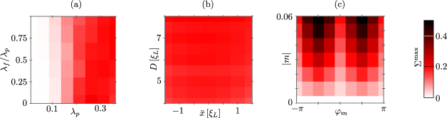
Figure 5: Values of $\Sigma^{\rm max}$ (in units of $e^{2}/h$), as a function of different parameters, in presence of a single magnetic impurity with strength $m$ and located at $x_{M}=2\xi_{L}$ (with $\xi_{L}=v/(\pi\Delta_{L})$). All the panels share the same color bar. In panel (a), we study the dependence of $\Sigma^{\rm max}$ on the tunneling amplitude $\lambda_{p}$ and on the ratio $\lambda_{f}/\lambda_{p}$ between spin-flipping and spin-preserving tunneling amplitudes at the QPC. Panel (b) highlights the very weak dependence of $\Sigma^{\rm max}$ on $D$ and $\bar{x}$ (both in units of $\xi_{L}$). In Panel (c), we consider different impurity strengths, by varying both the magnitude $|m|$ and the phase $\varphi_{m}=\arg(m)$. Each panel shares its fixed parameters with Fig. 3 of the main text, that is $D=6\xi_{L}$, $\Delta_{L}=\Delta,\Delta_{R}=1.2\Delta,\bar{x}=\xi_{L}$, $m=0.05$, $x_{\rm M}=2\xi_{L}$, $\lambda_{p}=0.25$, $\lambda_{f}=0.15$.

To better discuss the robustness of our analysis and stress the importance of sampling multiple points in parameter space, we numerically compute the maximum value of $|\Sigma|$ over the whole $(E-\chi)$ diagram, which we denote with $\Sigma^{\rm max}$, for several different scenarios. In Fig. 5, we consider the presence of a single magnetic impurity, as in Fig. 3 of the main text. We plot $\Sigma^{\rm max}$ for different combinations of parameters: $\lambda_{p}$ and $\lambda_{p}/\lambda_{f}$ [Fig. 5 (a)], $\bar{x}$ and $D$ [Fig. 5(b)], and $|m|$ and $\varphi_{m}=\arg(m)$ [Fig. 5(c)]. Note that $\varphi_{m}$ controls the direction of the impurity magnetization, which lies on the plane perpendicular to the spin quantization axis. These plots show the robustness of the results displayed in Fig. 3 of the main text, where we observe $\Sigma^{\rm max}\sim 0.2\,e^{2}/h$. The quantity $\Sigma^{\rm max}$ remains indeed considerably and consistently different from zero, with the exception of the trivial limits $|m|\to 0$ (i.e. without magnetic impurity) and $\lambda_{f},\lambda_{p}\to 0$ (i.e. without QPC).

In Fig. 6, we perform a similar analysis considering the presence of two magnetic impurities with strengths $m_{i}$ ($i=1,2$), each one described by the Hamiltonian $H_{\rm M}=2vm_{i}\,\psi_{\uparrow}^{\dagger}(x_{M_{i}})\psi_{\downarrow}(x_{M_{i}})+h.c.$ [see Eq. (65)], and located on the two sides of the QPC (i.e. $-D/2<x_{M_{1}}<\bar{x}<x_{M_{2}}<D/2$). In this case, we identify one specific scenario that results in $\Sigma=0$, even in presence of magnetic scatterers. It corresponds to the the fully symmetric configuration with real $m_{1}=m_{2}$, $\Delta_{L}=\Delta_{R}$, $\bar{x}=0$, and $x_{M_{2}}=-x_{M_{1}}$ (see the white spots in both panels of Fig. 6). Importantly, however, small deviations from this fine-tuned scenario lead to a rapid increase of $\Sigma^{\rm max}$ to detectable finite values. In particular, in Fig. 6(a), we show how variations in phase and magnitude of $m_{1}$, while keeping $m_{2}=0.5$ fixed, result in a finite $\Sigma^{\rm max}$. In Fig. 6(b), we show how, even for symmetric and real strengths $m_{1}=m_{2}=0.05$, it is still possible to get finite $\Sigma^{\rm max}$ just by changing the QPC position $\bar{x}$ and/or the position of one impurity ($x_{\rm M_{2}}$), while keeping the other one fixed at $x_{\rm M_{1}}=-2\xi_{L}$.

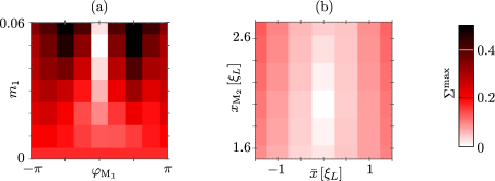
Figure 6: Values of $\Sigma^{\rm max}$ (in units of $e^{2}/h$), as a function of different parameters, in presence of two magnetic impurities, with strengths $m_{1}$ and $m_{2}$, located on both sides of the QPC (i.e $x_{M_{1}}<\bar{x}<x_{M_{2}}$). The two panels share the same color bar. In panel (a), we study the dependence of $\Sigma^{\rm max}$ on the strength of impurity $1$, by varying both its magnitude $|m_{1}|$ and phase $\varphi_{m_{1}}=\arg(m_{1})$, while keeping $m_{2}=0.05$ fixed. The QPC is at $\bar{x}=0$ and the impurities are located at $x_{\rm M_{2}}=-x_{\rm M_{1}}=2\xi_{L}$. In panel (b), we plot $\Sigma^{\rm max}$ as a function of the positions of the QPC ($\bar{x}$) and the impurity $2$ ($x_{\rm M_{2}}$), both in units of $\xi_{L}$, for $m_{1}=m_{2}=0.05$ and $x_{\rm M_{1}}=-2\xi_{L}$. Both panels share the remaining parameters, which read $D=6\xi_{L}$, $\Delta_{L}=\Delta_{R}=\Delta$, $\lambda_{p}=0.25$, $\lambda_{f}=0.15$.

Appendix E Magnetic impurity

Here, we consider the effect of a delta-like magnetic impurity along the upper helical edge, described by the Hamiltonian (we suppress the redundant index $r$)

$$H_{\rm M}=2vm\,\psi_{\uparrow}^{\dagger}(x_{M})\psi_{\downarrow}(x_{M})+h.c..$$ (65)

The equations of motion for the field operators, i.e. $i\partial_{t}\psi_{\sigma}=-[H_{\zeta=-1}+H_{\rm M},\psi_{\sigma}]$, become

$$i\partial_{t}\psi_{\uparrow} =+iv\partial_{x}\psi_{\uparrow}+2mv\delta(x-x_{M})\psi_{\downarrow}$$ (66)

$$i\partial_{t}\psi_{\downarrow} =-iv\partial_{x}\psi_{\downarrow}+2m^{*}v\delta(x-x_{M})\psi_{\uparrow}.$$ (67)

Using again the plane wave ansatz

$$\psi_{\sigma}(x)=\frac{e^{-iEt}}{\sqrt{\hbar v}}\begin{cases}\tau^{e}_{\sigma}e^{-i\sigma Ex/v}\qquad&\sigma(x-x_{M})>0\\ \omega^{e}_{\sigma}e^{-i\sigma Ex/v}\qquad&\sigma(x-x_{M})<0\end{cases},$$ (68)

we can relate the incoming ($\tau$) and outgoing amplitudes ($\omega$) as

$$i(\omega^{e}_{\uparrow}-\tau^{e}_{\uparrow}) =me^{2iEx_{M}/v}(\omega^{e}_{\downarrow}+\tau^{e}_{\downarrow})$$ (69)

$$i(\omega^{e}_{\downarrow}-\tau^{e}_{\downarrow}) ={m^{*}}e^{-2iEx_{M}/v}(\omega^{e}_{\uparrow}+\tau^{e}_{\uparrow}).$$ (70)

The resulting (electronic) scattering matrix reads

$$\begin{pmatrix}\omega^{e}_{\uparrow}\\ \omega^{e}_{\downarrow}\end{pmatrix}=\frac{1}{1+|m|^{2}}\begin{pmatrix}1-|m|^{2}&-2ie^{2iEx_{M}/v}m\\ -2ie^{-2iEx_{M}/v}m^{*}&1-|m|^{2}\end{pmatrix}\begin{pmatrix}\tau^{e}_{\uparrow}\\ \tau^{e}_{\downarrow}\end{pmatrix}.$$ (71)

We observe that, for $m=1$, the transmission coefficients vanish. In this limit, therefore, the magnetic impurity described by $H_{\rm M}$ induces perfect electronic backscattering (with spin-flip) at $x=x_{M}$. Introducing the hole amplitudes, we get

$$\begin{pmatrix}\omega^{e}_{\uparrow}\\ \omega^{e}_{\downarrow}\\ \omega^{h}_{\uparrow}\\ \omega^{h}_{\downarrow}\end{pmatrix}=S_{\rm M}(m,x_{M},E)\begin{pmatrix}\tau^{e}_{\uparrow}\\ \tau^{e}_{\downarrow}\\ \tau^{h}_{\uparrow}\\ \tau^{h}_{\downarrow}\end{pmatrix}$$ (72)

with

$$S_{\rm M}(m,x_{M},E)=\frac{1}{1+|m|^{2}}\begin{pmatrix}1-|m|^{2}&-2ie^{2iEx_{M}/v}m&0&0\\ -2ie^{-2iEx_{M}/v}m^{*}&1-|m|^{2}&0&0\\ 0&0&1-|m|^{2}&2ie^{2iEx_{M}/v}m^{*}&\\ 0&0&2ie^{-2iEx_{M}/v}m&1-|m|^{2}\\ \end{pmatrix}$$ (73)

Appendix F Properites of the non-local differential conductances

The aim of this section is to address the properties of the non-local differential conductances $G_{12/21}(E,\chi)$, with respect to the inversion of $E$ and/or $\chi$.

F.1 Energy inversion

From the observation of Fig. 2(a-c) in the main text, one can immediately notice the asymmetry $G_{12/21}(E,\chi)\neq G_{12/21}(-E,\chi)$. The latter stems precisely from the capability of our system to selectively detect only one class of hABS (and not its particle-hole symmetric partner, with opposite spin structure). This feature is strictly present for $\lambda_{f}=0$ [Fig. 2(a) of the main text]. However, the asymmetry survives also in presence of a weak to moderate $\lambda_{f}<\lambda_{p}$ [see Fig. 2(b,c) of the main text]. It disappears only for the special case $\lambda_{f}=\lambda_{p}$, i.e. when the tunneling at the QPC is completely spin insensitive and both classes of hABS give the same signal in the conductances.

F.2 Energy and phase inversion

Interestingly, in presence of perfect hABSs, the non-local differential conductance satisfy

$$G_{12/21}(E,\chi)=G_{12/21}(-E,-\chi).$$ (74)

This is a direct consequence of the energy-phase relation of each class of hABS [see Eq.(3) in the main text], which is indeed invariant under the transformation (note that the functions $\Phi_{r}$ are odd with respect to E)

$$\begin{cases}E\to-E\\ \chi\to-\chi.\end{cases}$$ (75)

At the mathematical level, we observe that the transformation (75) modifies the reflection coefficients at the QPC and at the superconducting interfaces as [see Eqs. (2) and Eqs. (32-36)]

$$S_{\rm QPC}(E,\lambda_{p},\lambda_{f}) =S_{\rm QPC}(-E,-\lambda_{p},-\lambda_{f})^{*}$$ (76)

$$\frac{\alpha^{c}_{r\sigma}}{\beta^{\tilde{c}}_{{\tilde{r}}{\tilde{\sigma}}}}\Big{|}_{(E,\chi)} =-\left[\frac{\alpha^{c}_{r\sigma}}{\beta^{\tilde{c}}_{{\tilde{r}}{\tilde{\sigma}}}}\Big{|}_{(-E,-\chi)}\right]^{*}.$$ (77)

Those changes are irrelevant for the computation of the absolute values of the transmission and reflection coefficients on the lower edge [i.e. $t,r,c,a$ in Eq. (5) in the main text and in Eq. (37)]. As a consequence, they have no effect on the differential conductances either, as confirmed by the analytical expressions of the coefficients in Eqs. (38-51).

The situation is different, however, in presence of additional scattering mechanisms on the upper edge. For the sake of concreteness, let us focus on the presence of magnetic impurities. In this case, the transformation (75) modifies the corresponding scattering matrix as $S_{\rm M}(E,m)=S_{\rm M}(-E,-m^{*})^{*}$ [see Eq. (73)]. Every amplitude appearing in Eq. (37) results from the interference of paths featuring different numbers of reflections on the magnetic impurity. As long as $m$ is not imaginary, therefore, the transformation $m\to-m^{*}$ modifies the interference and thus the differential conductances. This explains why, the relation $G_{12/21}(E,\chi)=G_{12/21}(-E,-\chi)$ does not hold in Fig. 3 of the main text. However, it is possible to construct scattering mechanisms that preserve Eq. (74) while still hybridizing and destroying the hABSs. It is the case, for example, for magnetic impurities with imaginary $m$, i.e. impurities with magnetization along the $y$ direction (assuming the spin quantization axis to be along $z$). Such a scenario is analyzed in Fig. 7, where we plot the differential conductances $G_{12/21/11}$ and $\Sigma$ using the same parameters considered in Fig. 3 of the main text, but with an imaginary $m=0.05\,i$. The two non-local conductances $G_{12/21}$ clearly satisfy Eq. (74), even in presence of magnetic scatterers. Importantly, the absence of hABSs is correctly signaled by the quantity $\Sigma$ [Fig. 7(d)], which features large deviations from zero.

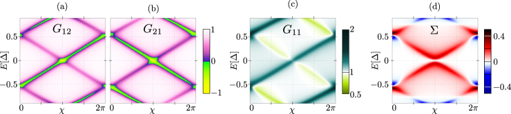
Figure 7: Differential conductances (in units of $e^{2}/h$) in presence of electronic backscattering on the upper edge, induced by a magnetic impurity with $m=0.05\,i$ and located at $x_{\rm M}=2\xi_{L}$ (with $\xi_{L}=v/(\pi\Delta_{L})$). The remaining parameters are the same as in Figs. 2(b,c) and 3 of the main text. They read $D=6\xi_{L}$, $\lambda_{p}=0.25$, $\lambda_{f}=0.15$, $\bar{x}=\xi_{L}$, $\Delta_{L}=\Delta$, $\Delta_{R}=1.2\Delta$.

References

König et al. (2007)M. König, S. Wiedmann,
C. Brüne, A. Roth, H. Buhmann, L. W. Molenkamp, X.-L. Qi, and S.-C. Zhang, Science 318, 766 (2007).
Aasen et al. (2016)D. Aasen, M. Hell,
R. V. Mishmash, A. Higginbotham, J. Danon, M. Leijnse, T. S. Jespersen, J. A. Folk, C. M. Marcus, K. Flensberg, and J. Alicea, Phys. Rev. X 6, 031016 (2016).
Gresta et al. (2021)D. Gresta, G. Blasi,
F. Taddei, M. Carrega, A. Braggio, and L. Arrachea, Phys. Rev. B 103, 075439 (2021).
Reis et al. (2017)F. Reis, G. Li, L. Dudy, M. Bauernfeind, S. Glass, W. Hanke, R. Thomale, J. Schäfer, and R. Claessen, Science (2017), 10.1126/science.aai8142.
Wu et al. (2018)S. Wu, V. Fatemi, Q. D. Gibson, K. Watanabe, T. Taniguchi, R. J. Cava, and P. Jarillo-Herrero, Science 359, 76
(2018).
Tang et al. (2017)S. Tang, C. Zhang,
D. Wong, Z. Pedramrazi, H.-Z. Tsai, C. Jia, B. Moritz, M. Claassen, H. Ryu, S. Kahn, J. Jiang,
H. Yan, M. Hashimoto, D. Lu, R. G. Moore, C.-C. Hwang, C. Hwang, Z. Hussain,
Y. Chen, M. M. Ugeda, Z. Liu, X. Xie, T. P. Devereaux, M. F. Crommie, S.-K. Mo, and Z.-X. Shen, Nature Physics 13, 683 (2017).
Li et al. (2018a)G. Li, W. Hanke, E. M. Hankiewicz, F. Reis, J. Schäfer, R. Claessen, C. Wu, and R. Thomale, Phys.
Rev. B 98, 165146
(2018a).
Pribiag et al. (2015)V. S. Pribiag, A. J. A. Beukman, F. Qu,
M. C. Cassidy, C. Charpentier, W. Wegscheider, and L. P. Kouwenhoven, Nature
Nanotechnology 10, 593
(2015).
Roth et al. (2009)A. Roth, C. Brune,
H. Buhmann, L. W. Molenkamp, J. Maciejko, X.-L. Qi, and S.-C. Zhang, Science 325, 294
(2009).
Brüne et al. (2012)C. Brüne, A. Roth,
H. Buhmann, E. M. Hankiewicz, L. W. Molenkamp, J. Maciejko, X.-L. Qi, and S.-C. Zhang, Nature
Physics 8, 485 (2012).
Hart et al. (2014)S. Hart, H. Ren, T. Wagner, P. Leubner, M. Mühlbauer, C. Brüne, H. Buhmann, L. W. Molenkamp, and A. Yacoby, Nature Physics 10, 638 (2014).
Wiedenmann et al. (2016)J. Wiedenmann, E. Bocquillon, R. S. Deacon, S. Hartinger,
O. Herrmann, T. M. Klapwijk, L. Maier, C. Ames, C. Brüne, C. Gould,
A. Oiwa, K. Ishibashi, S. Tarucha, H. Buhmann, and L. W. Molenkamp, Nature Communications 7 (2016), 10.1038/ncomms10303.
Bocquillon et al. (2016)E. Bocquillon, R. S. Deacon, J. Wiedenmann,
P. Leubner, T. M. Klapwijk, C. Brüne, K. Ishibashi, H. Buhmann, and L. W. Molenkamp, Nature
Nanotechnology 12, 137
(2016).
Bocquillon et al. (2018)E. Bocquillon, J. Wiedenmann, R. S. Deacon, T. M. Klapwijk, H. Buhmann, and L. W. Molenkamp, in Topological Matter (Springer
International Publishing, 2018) pp. 115–148.
Laroche et al. (2019)D. Laroche, D. Bouman,
D. J. van Woerkom,
A. Proutski, C. Murthy, D. I. Pikulin, C. Nayak, R. J. J. van Gulik, J. Nygård, P. Krogstrup, L. P. Kouwenhoven, and A. Geresdi, Nat. Commun. 10, 245 (2019).
Dartiailh et al. (2021)M. C. Dartiailh, J. J. Cuozzo, B. H. Elfeky,
W. Mayer, J. Yuan, K. S. Wickramasinghe, E. Rossi, and J. Shabani, Nat
Commun 12, 78 (2021).
de Vries et al. (2018)F. K. de Vries, T. Timmerman,
V. P. Ostroukh, J. van Veen, A. J. A. Beukman, F. Qu, M. Wimmer, B.-M. Nguyen, A. A. Kiselev, W. Yi, M. Sokolich,
M. J. Manfra, C. M. Marcus, and L. P. Kouwenhoven, Phys. Rev. Lett. 120, 047702 (2018).
de Vries et al. (2019)F. K. de Vries, M. L. Sol,
S. Gazibegovic, R. L. M. o. Veld, S. C. Balk, D. Car, E. P. A. M. Bakkers, L. P. Kouwenhoven, and J. Shen, Phys. Rev. Research 1, 032031(R) (2019).
Haidekker Galambos et al. (2020)T. Haidekker Galambos, S. Hoffman, P. Recher,
J. Klinovaja, and D. Loss, Phys. Rev. Lett. 125, 157701 (2020).
Vigliotti et al. (2022)L. Vigliotti, A. Calzona,
B. Trauzettel, M. Sassetti, and N. T. Ziani, “Anomalous flux periodicity in proximitised
quantum spin hall constrictions,” (2022), arXiv:2201.03259 [cond-mat.mes-hall]
.
Danon et al. (2020)J. Danon, A. B. Hellenes,
E. B. Hansen, L. Casparis, A. P. Higginbotham, and K. Flensberg, Phys. Rev. Lett. 124, 036801 (2020).
Nichele et al. (2017)F. Nichele, A. C. C. Drachmann, A. M. Whiticar, E. C. T. O’Farrell, H. J. Suominen, A. Fornieri,
T. Wang, G. C. Gardner, C. Thomas, A. T. Hatke, P. Krogstrup, M. J. Manfra, K. Flensberg, and C. M. Marcus, Phys. Rev. Lett. 119, 136803 (2017).
Schindele et al. (2014)J. Schindele, A. Baumgartner, R. Maurand, M. Weiss, and C. Schönenberger, Phys. Rev. B 89, 045422 (2014).
Strunz et al. (2019)J. Strunz, J. Wiedenmann,
C. Fleckenstein, L. Lunczer, W. Beugeling, V. L. Müller, P. Shekhar, N. T. Ziani, S. Shamim, J. Kleinlein, H. Buhmann, B. Trauzettel, and L. W. Molenkamp, Nature
Physics 16, 83 (2019).
(58)We assume the superconducting regions to be
much larger than the superconducting coherence lengths ( is the Fermi velocity) so that the upper helical edge is
completed decoupled from other gapless parts of the 2DTI on the outer side of
each superconducting electrode.
Li et al. (2018b)C. Li, J. C. de Boer,
B. de Ronde, S. V. Ramankutty, E. van Heumen, Y. Huang, A. de Visser, A. A. Golubov, M. S. Golden, and A. Brinkman, Nature Materials 17, 875 (2018b).
Murani et al. (2017)A. Murani, A. Kasumov,
S. Sengupta, Y. A. Kasumov, V. T. Volkov, I. I. Khodos, F. Brisset, R. Delagrange, A. Chepelianskii, R. Deblock, H. Bouchiat, and S. Guéron, Nature Communications 8 (2017), 10.1038/ncomms15941.
(71)Note that our setup is effectively a
multi-terminal device, featuring two metallic and two superconducting
electrodes. The latter ones can act as sinks/sources of pairs of electrons
via Andreev reflection.
(72)Note that Andreev transmission processes
necessarily involve both spin-preserving and spin-flipping tunnelings. Hence,
for , we have and .
(74)Since we consider
and finite junction lengths in order to accomodate the QPC (e.g.
in Figs. 2 and 3), we expect to find ABS for all the values of the phase
difference Chang and Bagwell (1994).
Fleckenstein et al. (2021)C. Fleckenstein, N. T. Ziani, A. Calzona,
M. Sassetti, and B. Trauzettel, Phys. Rev. B 103, 125303 (2021).
(76)“See supp. material.” .
(77)Strictly speaking, the observation of
implies either (i.e. pure electronic
backscattering) or (i.e. pure AR). It is however
straightforward to distinguish between these to limits. For example, in
presence of pure electronic backscattering, no Andreev processes are present
and cannot be negative. Moreover, in this case, the
superconductors should not play any role and the conductances are thus
expected not to depend on .