CloudRCA: A Root Cause Analysis Framework
for Cloud Computing Platforms

Abstract.

As business of Alibaba expands across the world among various industries, higher standards are imposed on the service quality and reliability of big data cloud computing platforms which constitute the infrastructure of Alibaba Cloud. However, root cause analysis in these platforms is non-trivial due to the complicated system architecture. In this paper, we propose a root cause analysis framework called CloudRCA which makes use of heterogeneous multi-source data including Key Performance Indicators (KPIs), logs, as well as topology, and extracts important features via state-of-the-art anomaly detection and log analysis techniques. The engineered features are then utilized in a Knowledge-informed Hierarchical Bayesian Network (KHBN) model to infer root causes with high accuracy and efficiency. Ablation study and comprehensive experimental comparisons demonstrate that, compared to existing frameworks, CloudRCA 1) consistently outperforms existing approaches in f1-score across different cloud systems; 2) can handle novel types of root causes thanks to the hierarchical structure of KHBN; 3) performs more robustly with respect to algorithmic configurations; and 4) scales more favorably in the data and feature sizes. Experiments also show that a cross-platform transfer learning mechanism can be adopted to further improve the accuracy by more than 10%. CloudRCA has been integrated into the diagnosis system of Alibaba Cloud and employed in three typical cloud computing platforms including MaxCompute, Realtime Compute and Hologres. It saves Site Reliability Engineers (SREs) more than $20\%$ in the time spent on resolving failures in the past twelve months and improves service reliability significantly.

1. Introduction

Nowadays, tens of millions of products and billions of consumers are involved in Alibaba’s e-commerce platforms. A tremendous amount of data at PB-level is processed every day on Alibaba’s big data cloud computing platforms, in order to complete transactions and provide appropriate recommendations to customers. The number of merchants, consumers, daily processed data still keep increasing and reach its peak on the Double 11 global shopping festival every year. Therefore, stability and fast fault recovery of cloud platforms are essential for supporting these business scenarios.

The main challenges of root cause identification for big data cloud computing platforms at Alibaba include: (1) The ever increasing scale and complexity of computing platforms as well as multi-source, large-volume and unstructured data make it difficult for SREs to perform troubleshooting manually; (2) Real-time business scenarios are ubiquitous and time-sensitive, hence the whole process of detection and diagnosis needs to be finished in a faster way, for which efficiency is usually measured by MTTR (Mean Time to Resolve); (3) Faults are relatively rare in those systems, which limit the amount of samples available for training models; (4) Due to the diversity of Alibaba’s business scenarios, there are different kinds of computing platforms serving various requests, such as large-scale batch computing, real-time computing, interactive analysis, etc. Therefore the root cause analysis workflow needs to be widely applicable to computing platforms with different architectures.

There are several well-studied root cause analysis (RCA) methods that have been demonstrated to perform competitively, such as CloudRanger proposed in (Wang et al., 2018) from IBM, OM knowledge graph based method (O&M Graph for short) proposed by (Qiu et al., 2020), and LogCluster proposed by (Lin et al., 2016b) from Microsoft. These methods utilize either KPI time series or logs for root cause analysis, however, none of them uses these two important sources of data at the same time. Moreover, none of these methods provides direct root cause types which can guide SREs or automatic tools to take actions and recover the systems without further manual investigation. Specifically, in CloudRanger and O&M Graph, the root cause inference result is the KPI node on the graph, while for LogCluster, the inference result is the representative log sequences.

In this paper, we propose a root cause analysis workflow called CloudRCA, and the main contributions of our study are: (1) The framework integrates multiple sources of data including not only monitoring metrics but also system logs together with expert knowledge, resulting in higher accuracy compared with other methods that only consider KPIs or logs. We also improve the algorithms used in CloudRCA, such as optimizing the pruning strategy in log template extraction, improving log clustering through Natural Language Processing feature representations and defining the hierarchical root cause layers based on traditional Bayesian networks, all leading to higher accuracy and efficiency of CloudRCA than existing RCA methods. This has been demonstrated through comprehensive experiments in our study. (2) CloudRCA is able to deal with brand new types of root causes that have never been seen before, thanks to the innovative design of hierarchical root cause layer in the Bayesian network. This improvement in Bayesian network enables the model to infer the most likely root cause module even when encountered with new types. (3) CloudRCA is a general framework that can be easily deployed on various cloud systems with minor adaptations. It has been implemented on Alibaba’s three big data cloud computing platforms in practice, namely MaxCompute, Realtime Compute and Hologres, and helps SREs reduce the time of resolving failures by more than 20% in the past twelve months. (4) A comprehensive set of experiments are conducted, from which key insights regarding RCA modeling are derived.

2. Related work

Many research papers on RCA focus on complex large-scale systems (Qiu et al., 2020; Thalheim et al., 2017; Weng et al., 2018). They can be grouped into the following categories:

2.0.1. Log-based methods

The common methodology to RCA is to analyze log files to identify problems that occurred in the system. The problems are then examined to identify potential causes. (Lin et al., 2016a) introduced a classic log mining method to diagnose and locate anomalies in distributed systems. According to (Xu et al., 2017; Jia et al., 2017), the log mining method also plays an important role in the RCA of cloud applications. However, the limited coverage of log features makes it difficult for methods relying only on log features to achieve high accuracy.

2.0.2. Correlation analysis-based methods

These methods correlate events, metrics and alerts to locate the root cause of an anomaly or failure. (Zeng et al., 2014) proposed a parametric model to describe noisy time lags from fluctuating events. (Marvasti et al., 2013) introduced a model of statistical inference to manage complex infrastructures based on their anomalous events data obtained from an intelligent monitoring engine. But without considering the topology of infrastructures and other domain knowledge, the correlated results may be hard for SREs to understand.

2.0.3. DAG-based methods

Deploying applications in cloud environments has become a tendency. As calls between systems become more and more complex, it is difficult for SREs to directly locate root causes. In the RCA research for cloud applications, the most representative are related studies from CloudRanger (Wang et al., 2018) from IBM and OM knowledge graph based method (Qiu et al., 2020). These methods build a dependency or causality graph from historical KPIs data and use the constructed graph to infer root causes online. But those works don’t make full use of expert knowledge and multiple sources of data including logs.

3. Proposed CloudRCA Framework

Our framework features a novel integration of three sources of information, including metrics from monitoring system, log messages from logging system, and module dependency relationship in Configuration Management Database (CMDB). An overview is shown in Figure 1. First, in the feature engineering stage, data from multiple sources are converted into unified feature matrices through time series anomaly detection and log clustering algorithms. Then a KHBN(Knowledge-informed Hierarchical Bayesian Network), combining processed signal data and domain knowledge of module dependency, is built to infer root causes in real time. Next we elaborate on each component of the framework.

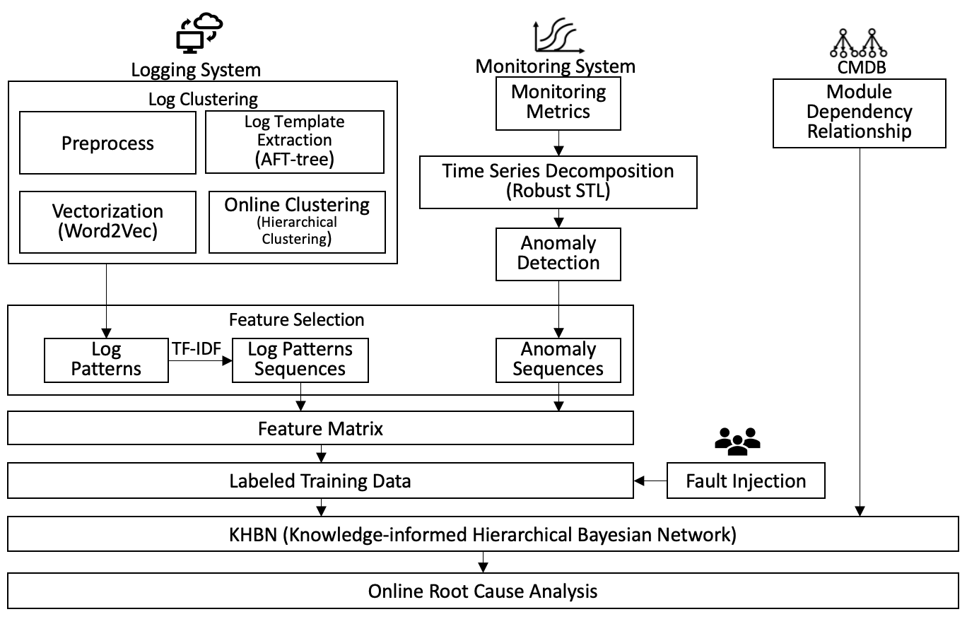
Figure 1. The workflow of the proposed CloudRCA framework.

3.1. Metrics Anomaly Detection

This subsection presents the extraction of anomalous metrics collected from monitoring systems as a basis for RCA. Based on the analysis of historical failure data in our cloud computing platforms, we summarize four kinds of typical anomalies that are frequently related to system breakdowns, including spikes and dips, change of mean, change of variance, and long-term trend. We design a decomposition-based scheme to detect these anomalies.

We first identify period lengths of the time-series metrics. Since metrics in stream processing typically exhibit daily and/or weekly periodicity, we design a simplified RobustPeriod algorithm (Wen et al., 2021) which adopts wavelet transform to isolate single periodicity and then identifies the exact period from the peaks of the auto-correlation function (ACF). Next, we decompose the time series into tread, seasonality, and remainder components. Traditional STL (Seasonal-Trend decomposition using Loess) proposed in (Robert et al., 1990) suffers from less flexibility when seasonality period is long and is vulnerable to noises. Therefore we use a novel and robust decomposition method called RobustSTL (Wen et al., 2019, 2020; Yang et al., 2021). RobustSTL first extracts the trend component by solving a regression problem using the least absolute deviation loss with sparse regularization, then estimates the seasonality component with a non-local seasonal filtering.

With the decomposed time series, we identify those anomalies in a “divide-and-conquer” manner, as summarized in Table 1. The main idea is to detect different types of anomalies from different components using proper statistical tests. Furthermore, two improvements are adopted for practical considerations. First, robust statistics (Zoubir et al., 2012), such as median and median absolute deviation (Leys et al., 2013) in place of simple mean and variance (Hochenbaum et al., 2017), are utilized in the statistical tests to hedge against outliers and noises in time series. Second, online versions of these tests are implemented by updating statistics incrementally via a bisection algorithm (Ali et al., 2017), which greatly boosts the computational speed.

Table 1. Summary of the designed decomposition-based anomaly detection scheme.

Anomaly Type	Component	Statistical Test
Spikes & Dips	remainder	Extreme studentized deviate test
Change of Variance	remainder	F-test
Change of Mean	trend	T-test
Long-term Trend	trend	Mann-Kendall test

3.2. Log Templates Extraction and Clustering

Apart from monitoring metrics, numerous logs are consistently produced by many different modules that constitute a large-scale cloud computing platform. The sheer volume, varying syntax and semantics across modules make log analysis a non-trivial task. This section describes an effective template extraction method and pattern clustering that aggregates the vast raw log messages into several representative patterns.

After a standard log preprocessing process, including stemming and case-folding, we extract templates from message contents by removing variables such as IP address, table name, interface IDs, etc., that are not critical in diagnosis.

We develop an incrementally trainable algorithm called Adaptive Frequent Template tree (AFT-tree) based on FT-tree (Zhang et al., 2018) to obtain log templates automatically instead of using regular expression. AFT-tree is designed with better efficiency and adaptivity. First, we use dictionaries to store children of nodes instead of lists, and avoid duplicated searching while inserting nodes. Our approach turns out $27$ times faster than FT-tree on our datasets. Second, unlike FT-tree that prunes the tree based on the number of children, AFT-tree uses the number of leaves of a node for pruning so that the template length can adapt to the length of the log to capture important non-variables.

After extracting the structural templates of the logs, we cluster them by the semantics with NLP algorithms. We apply Word2vec (Mikolov et al., 2013a; Mikolov et al., 2013b) to obtained vector-representations of the logs. Then we perform hierarchical clustering (Gower and Ross, 1969) based on the cosine similarity between the vectors to aggregate logs into different clusters, which we call log patterns.

Since logs are constantly generated, our clustering algorithm needs to run in an efficient online mode. To this end, we first conduct an offline training to obtain the clusters. For each cluster, we select a representative log by choosing the center of the cluster. To be precise, we compute a score for each log in a cluster based on its average distance to other logs within the same cluster:

$$\textrm{Score}(i)=\frac{1}{n-1}\sum_{j=1}^{n}(1-\textrm{similarity}(\text{log}_{i},\text{log}_{j}))$$

where $n$ is the total number of logs in the cluster, and the log content with the minimum score is selected as the representative. Then in the online mode, new logs are clustered together with the extracted representatives, where they either get distributed into the existing clusters or form new ones by their own. To be more specific, when a new log $s$ comes, we compute the similarity of the input log $s$ with the representatives of existing clusters. If the similarity is above a threshold $\theta$, we assign the input log message to the cluster with the greatest similarity; otherwise we create a new cluster for $s$, with $s$ itself as the representative. In practice, the threshold can be calculated as:

$$\textrm{$\theta$}=\frac{1}{m}\sum_{i=1}^{m}\textrm{average\_similarity\_cluster}_{i}$$

where $m$ is total number of clusters, and $\textrm{average\_similarity\_cluster}_{i}$ is the average similarity of the representative log of cluster $i$ with other logs in cluster $i$.

3.3. Knowledge-informed Hierarchical Bayesian Network (KHBN)

In addition to logs and monitoring metrics, we also have tree-based data stored in Configuration Management Database (CMDB) which describe complicated dependency relationships between modules and root cause types that are useful for issue-tracking but hard to infer otherwise. All these are integrated into RCA through a hierarchical Bayesian network.

To prepare for network construction, we transform the logging and monitoring data into standard feature data. We build time series for log patterns indicating whether a certain log pattern appears (marked $1$) or not (marked $0$). Similarly, each monitoring item is marked $1$ if it’s deemed as an anomaly by the algorithm and $0$ otherwise. For convenience, both transformed series are called metrics in our network. Some metrics may not be valuable for root cause identification and adversely affect the model, therefore we calculate the TF-IDF score of each feature to select only the most informative ones.

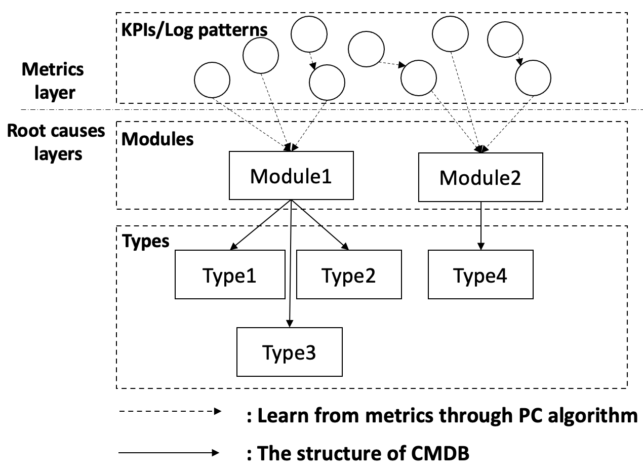
Figure 2. The structure of the proposed KHBN diagram.

The structure of KHBN is shown in Figure 2. The nodes of the first layer are metrics selected from logging and monitoring, and root cause layer is composed of module-level nodes as well as type-level nodes. We build the network structure in two phases, an allocation phase and a causal learning phase. In the allocation phase, we use topology information from CMDB to generate the initial edges between nodes. In the causal learning phrase, directed edges that represent causal relationship between nodes are constructed based on system metrics collected from both normal and abnormal periods. This is achieved by the PC algorithm (Wang et al., 2018), a standard method for estimating causal structures. After constructing the network structure, we calculate the conditional probability table of each node using the maximum likelihood estimate. In this way we obtain a complete Bayesian network that incorporates CMDB topology and system historical metrics. The network can be updated regularly as new data are collected. We then identify the root cause type through exact inference. When system fails, we input those feature data into KHBN model we trained with historical data, and select the node from the root cause types layer with the highest probability as the root cause, which is defined as

$$t_{i}^{*}=\textrm{argmax}_{t_{i}}\;P(t_{i}|m_{k},s_{1},s_{2},...,s_{j})P(m_{k}|s_{1},s_{2},...,s_{j})$$

where $t_{i}$ stands for a certain type of root cause, $m_{k}$ is the node in the module layer that points to $t_{i}$, and $s_{1},\ldots,s_{j}$ represent the observed nodes in the first layer. $t_{i}^{*}$ is the root cause type inferred by our model which has the highest conditional probability.

4. Real-World Deployments

Our root cause localization workflow is deployed in several big data cloud computing platforms of Alibaba, including MaxCompute, Realtime Compute and Hologres. The evaluation starts with the illustration of the importance of each step in the workflow, followed by the comparison of the algorithms we take in each phase with other state-of-art algorithms, and we also compare and analyze the performance on those three platforms. We then demonstrate the advantage of CloudRCA in dealing with brand new types of root causes, analyze the effect of eliminating predefined knowledge and assess the effectiveness of transfer learning in our workflow. Sensitivity study and overhead analysis are also performed. In Section 4.7, we share three real-world cases during the employment of CloudRCA on three platforms.

4.1. Cloud Computing Platforms at Alibaba

4.1.1. MaxCompute

MaxCompute is a data processing platform for large-scale data warehousing. It has been widely used and trusted by Alibaba and other customers, and is responsible for various large-scale data analysis scenarios in e-commerce, security, manufacturing and logistics. Currently, MaxCompute has more than 100 thousand servers located in data centers around the world, and can process more than one million jobs each day. The stored data has reached EB-level data volume long before, making it one of the leading products in the global market. The system architecture of MaxCompute is very similar to those of other big data computing engines in the industry. The most underlying is the infrastructure including host, network and so on. The storage module is a hierarchical storage distributed file system called Pangu. The resource management module is a scheduler with decentralized multi-scheduler architecture, which was designed to schedule large-scale distributed resources and improve cluster utilization.

4.1.2. Realtime Compute

Realtime Compute offers a one-stop, high-performance platform that enables real-time big data processing based on Apache Flink. It not only provides internal services at Alibaba, but also supports Flink-based cloud products in the entire developer ecosystem by using cloud product APIs at Alibaba Cloud, and has become a popular stream computing engine even the de facto standard in the real-time computing industry domestically and internationally. The number of Alibaba Cloud’s real-time computing jobs has reached more than 35,000 with the computing scale over 1.5 million CPUs, and the peak of real-time data processing during this year’s Double 11 reached 4 billion records per second. Flink computing engine runs on open-source Hadoop clusters. YARN of Hadoop is used for resource management and scheduling, and HDFS is used for data storage.

4.1.3. Hologres

Hologres is a cloud-native Hybrid Serving & Analytical Processing (HSAP) system that is seamlessly integrated with the big data ecosystem. It integrates the processes of analytical processing and knowledge serving and supports highly concurrent writes and queries at a speed of up to 100 million transactions per second (TPS). Hologres takes a cloud-native design architecture where the computation and storage layers are decoupled. The computing module is deployed on Kubernetes while the storage layer is Pangu by default, which is a high performance distributed file system, similar to MaxCompute.

The three platforms above are typical representatives of the big data ecosystem at Alibaba. They serve different purposes of data processing and analysis and vary in scale. Despite the diversity in compute engine, scheduler and storage module design, they share some infrastructure such as host, network, and their basic system modules are similar. Table 2 shows the modules and corresponding root cause types of the three platforms. It’s worth mentioning that all the three platforms have a trend toward the cloud-native data computing service, which means that they may share more infrastructure in storage and resource scheduler in the near future. The main differences among the three platforms are summarized in Table 3.

Table 2. System Modules and Corresponding Root Cause Types of the Three Platforms

Module	Realtime Compute	MaxCompute	Hologres
	Root Cause Types
Resource Scheduler	YARN NM decommissioned	Fuxi master fail	ASI server overload
	YARN RM switch	Fuxi tobo fail	ASI node fail
	YARN resource preemption	Fuxi apiserver overload	ASI apiserver overload
	…	…	…
Storage	HDFS service unavailable	pangu server unavailable
	HDFS usage over limit	pangu master failover
	HDFS call queue full	pangu master queue size full
	…	pangu server write slow
		pangu chunkserver failover
		…
Host	oom
	io hang
	disk failure
	cpu usage over limit
	machine breakdown
	…
Network	Martnet exception
	QoS exception
	LVS exception
	…
Other	Upstream-TT	Tunnel	POP
	Upstream-SLS	Frontend	DNS
	…	…	…

Table 3. Comparison of the Three Platforms

Module	RealtimeCompute	MaxCompute	Hologres
feature of compute engine	batch	stream	Hybrid Serving & Analytical Processing
cluster scale	MaxCompute >RealtimeCompute >Hologres
resource scheduler	YARN	Fuxi	ASI
storage	HDFS	Pangu	Pangu

4.2. Dataset and Setup

Related data over the past five years, including time series metrics, logs and tree-based data from CMDB, are collected for each platform. A summary of the data is shown in Table 4. We extract positive samples when the system is running normally and negative samples when the systems fail, including real faults and injected faults. All the positive samples are used as training set, which can help learn some correlation among those metrics, while negative samples are split into training set and test set with 60-40 ratio. As we can see from the Table, MaxCompute has the most negative samples due to its large scale and long-term data accumulation, while the dataset of Hologres are relatively small since it’s a fairly new product.

To evaluate the performance of CloudRCA and other root cause analysis models, we use precision, cover rate, and f1-score, which are defined as:

$$precision=\sum_{i}^{n}precision\_of\_each\_type(i)/n$$

$$cover\_rate=covered\_types/all\_types$$

$$f1\_score=2*precision*cover\_rate/(precision+cover\_rate)$$

precision_of_each_type(i) represents the percentage of samples that are correctly predicted for a certain root cause type i. The precision is the average of all types’ precision. It’s worth mentioning that a type is called covered when $\geq 60\%$ of testing samples in this type are correctly predicted. cover_rate indicates the covered types out of all types. f1_score is a composite indicator that balances precision and cover_rate.

Our workflow is parallel, and all experiments are run on up to four machines, each with 16 Intel Xeon E5-2650 @2.00GHz cores and 128GB RAM, running Debian GNU/Linux9.4.

Table 4. The Dataset of the three cloud computing platforms

Production	Module	Training Set		Testing Set
		Positive Samples	Negative Samples	Negative Samples
MaxCompute	Storage	861	123	82
	Resource Scheduler	924	132	88
	Host	798	114	76
	Network	777	111	74
	Other	840	120	80
Realtime Compute	Storage	273	39	26
	Resource Scheduler	287	41	27
	Host	455	65	43
	Network	378	54	36
	Other	189	27	18
Hologres	Storage	140	20	13
	Resource Scheduler	168	24	16
	Host	252	36	24
	Network	182	26	17
	Other	105	15	10

4.3. Ablation Study

We design experiments to study the contribution of different components of the proposed framework to the overall performance. We also compare the techniques we used at each stage with their alternatives to demonstrate their strengths.

4.3.1. Validation of Feature Engineering

The feature engineering stage in our workflow combines multi-source data and extracts the most relevant features. To demonstrate its effectiveness, we conduct experiments on each of the three platforms. For each step (i.e., anomaly detection, log template extraction, and log clustering) in feature engineering, we investigate two settings where: 1) the exact proposed method is used; 2) the step is not performed at all. Results are shown in Table 5. Note that “NONE” in the table stands for the setting where the particular step is skipped. For example, in the 3rd row of Table 5 anomaly detection is not performed, and the original kpi metrics are directly used to build KHBN, the root cause inference network.

Table 5. Ablation analysis

Production	Anomaly detection	Log template extraction	Is clustering	Precision	Cover rate	Time	Num of nodes	F1
MaxCompute	ROBUST STL	AFT-TREE	Hierarchical Clustering	79.8%	77.8%	3.2min	224	0.78
	NONE	AFT-TREE	Hierarchical Clustering	24.0%	33.3%	2.7min	224	0.27
	ROBUST STL	NONE	Hierarchical Clustering	38.1%	33.30%	17.3min	224	0.35
	ROBUST STL	AFT-TREE	NONE	19.8%	38.9%	57min	724	0.26
RealtimeCompute	ROBUST STL	AFT-TREE	Hierarchical Clustering	76.3%	72.2%	2.2min	173	0.74
	NONE	AFT-TREE	Hierarchical Clustering	30.2%	33.3%	1.8min	173	0.31
	ROBUST STL	NONE	Hierarchical Clustering	36.5%	33.30%	18.1min	173	0.34
	ROBUST STL	AFT-TREE	NONE	23.9%	33.3%	46min	651	0.27
Hologres	ROBUST STL	AFT-TREE	Hierarchical Clustering	60%	72.2%	1.7min	154	0.65
	NONE	AFT-TREE	Hierarchical Clustering	30.2%	50%	2.1min	154	0.37
	ROBUST STL	NONE	Hierarchical Clustering	36.5%	33.30%	14.7min	154	0.34
	ROBUST STL	AFT-TREE	NONE	16.7%	50%	37min	584	0.25

The results in Table 5 show that skipping any of the steps in the feature engineering workflow compromises the performance on all the platforms. The performance gain from anomaly detection, log template extraction and log clustering can be explained by fact that our feature engineering flow extracts the most relevant information from complex raw data and thus boosts the efficiency of KHBN in both graph construction and root cause inference.

4.3.2. Comparison of Different Techniques in Feature Engineering

In this part of our experiments, a benchmark method is used in place of the proposed at each stage of feature engineering. Specifically, for time series decomposition, we compare Robust STL with traditional STL (Robert et al., 1990), and for metric anomaly detection we compare the technique we proposed with Isolation Forest (iForest), an unsupervised detection algorithm proposed by (Liu et al., 2008). We compare AFT-tree with FT-tree (Zhang et al., 2018) in extracting log templates. As for log clustering, we use DBSCAN (Ester et al., 1996) as a surrogate for hierarchical clustering.

Table 6. Performance of different methods in feature engineering

Production	Anomaly detection	Log template extraction	Is clustering	Precision	Cover rate	Time	Num of nodes	F1
MaxCompute	ROBUST STL	AFT-TREE	Hierarchical Clustering	79.8%	77.8%	3.2min	224	0.78
	STL	AFT-TREE	Hierarchical Clustering	58.4%	61.1%	5.3min	224	0.60
	iForest	AFT-TREE	Hierarchical Clustering	48.9%	50%	4.7min	224	0.49
	ROBUST STL	FT-TREE	Hierarchical Clustering	55.2%	61.1%	83.2min	224	0.58
	ROBUST STL	AFT-TREE	DBSCAN	72.4%	77.80%	3.3min	224	0.75
RealtimeCompute	ROBUST STL	AFT-TREE	Hierarchical Clustering	76.3%	72.2%	2.2min	173	0.74
	STL	AFT-TREE	Hierarchical Clustering	48.9%	61.1%	4.2min	173	0.54
	iForest	AFT-TREE	Hierarchical Clustering	37.5%	61.1%	3.5min	173	0.46
	ROBUST STL	FT-TREE	Hierarchical Clustering	63.5%	72.2%	61.6min	173	0.67
	ROBUST STL	AFT-TREE	DBSCAN	73.2%	72.2%	2.4min	173	0.72
Hologres	ROBUST STL	AFT-TREE	Hierarchical Clustering	60%	72.2%	1.7min	154	0.65
	STL	AFT-TREE	Hierarchical Clustering	55.2%	61.1%	3.4min	154	0.58
	iForest	AFT-TREE	Hierarchical Clustering	42.7%	61.1%	2.9min	154	0.50
	ROBUST STL	FT-TREE	Hierarchical Clustering	43.8%	72.2%	42.5min	154	0.54
	ROBUST STL	AFT-TREE	DBSCAN	58.4%	72.2%	1.5min	154	0.64

Table 6 shows that (1) Robust STL leads to significant improvement over traditional STL in both performance and efficiency; (2) The anomaly detection technique we proposed outperforms iForest in all the metrics on all the platforms; (3) AFT-tree exhibits higher computational efficiency than FT-tree, thanks to the improved storage structure and pruning strategy; (4) As for log clustering, DBSCAN and hierarchical clustering perform similarly, indicating that other decent clustering methods may be employed as a substitute of hierarchical clustering.

4.3.3. Evaluation of KHBN

In this part of our experiments, we aim to compare the proposed root cause analysis algorithm KHBN with other well studied methods, including CloudRanger, OM knowledge graph based method (OM Graph for short) as well as LogCluster. CloudRanger takes advantage of a dynamic causal relationship analysis approach to construct impact graphs amongst applications without topology knowledge, and then uses a heuristic algorithm based on second-order random walk to identify the root cause metrics on the graph. OM Graph is an approach proposed by Juan Qiu etc. for mining causality and diagnosing root causes that uses knowledge graph technology and a causal search algorithm. LogCluster is an approach that clusters the logs and extracts representative log sequences from the clusters to identify a problem. A comparison of the four methods is summarized in Table 7. Note that KHBN, OM Graph and CloudRanger are all graph-based models with different construction principles and inference methodologies. For OM Graph and CloudRanger, the inferred root causes are the services on the graph which in our case correspond to the engineered features, and the precision are labeled by experienced SREs of the cloud platforms. We conduct comparative tests using the four methods on all the three cloud computing platforms and the results are listed in Table 8.

Table 7. Comparison among different root cause analysis methods

Method	KHBN	LogCluster	CloudRanger	OM Graph
knowledge-based	Yes	No	No	Yes
Graph-based	Yes	No	Yes	Yes
Nodes in the Graph	KPIs, Log patterns, root cause module and types	-	KPIs	KPIs
graph construction method	PC algorithm	-	causal analysis	causal analysis and optimized PC algorithm
inference method	exact inference	Clustering	Random walk	BFS algorithm
inference result	the most likely root cause module and types	representative log sequences	top k candidates of root cause	candidate root cause paths

Table 8. Performance of the four root cause analysis methods

Production	Framework of RCA	Precision	Cover rate	F1	Time
Max- Compute	KHBN	79.8%	77.8%	0.78	13.5s
	LogCluster	44.7%	38.9%	0.41	7.4s
	CLOUDRANGER	63.5%	61.1%	0.62	17.3s
	OM GRAPH	61.3%	33.3%	0.43	15.4s
Realtime- Compute	KHBN	76.3%	72.2%	0.74	11.2s
	LogCluster	43.8%	33.3%	0.37	6.3s
	CLOUDRANGER	70.8%	61.1%	0.65	12.8s
	OM GRAPH	66.7%	38.9%	0.49	13.6s
Hologres	KHBN	60%	72.2%	0.65	9.7s
	LogCluster	50%	50%	0.5	5.7s
	CLOUDRANGER	44.5%	33.3%	0.38	11.9s
	OM GRAPH	58.7%	38.9%	0.46	13.7s

The experimental results show that KHBN significantly outperforms LogCluster on all the three platforms. The reason lies in that LogCluster only considers logs and neglects information from KPIs as well as topology. KHBN outperforms CloudRanger and OM Graph in all the three platforms for at least 0.09 increase in f1 score. Among the three platforms, MaxCompute has the highest f1 score which reaches 0.78 because it has the richest historical data for training. We also find that KHBN is the fastest one in building the network model and inferring the root causes, since it’s computation is designed to be parallel.

4.3.4. The Impact of Predefined Knowledge

As we know from Table 9, both KHBN and OM Graph are built based on predefined knowledge which is the topology information from CMDB. In real-world cloud systems, however, it may not be easy to acquire complete topology knowledge to build the graph. Therefore we design experiments to study the impact of predefined knowledge on the performance of the four root cause analysis methods mentioned in Section 4.3.3 by eliminating some pre-known relationships between metrics and modules. The results are displayed in Table 9, which indicates that the f1 score of KHBN are lowered slightly when deployed in Realtime Compute and Hologres, while the performance of OM Graph deteriorates significantly. However, when it comes to MaxCompute, which has adequate training data, both of these two methods have robust performance in identifying the root cause. Therefore, eliminating predefined knowledge in the stage of constructing the model may adversely affect the performance, but the performance drop can be partially offset by the availability of sufficient training data.

Table 9. Performance of the models having predefined knowledge

Production	Predefined knowledge	Framework RCA	Precision	Cover rate	F1	Time
Max- Compute	CMDB	KHBN	79.8%	77.8%	0.78	13.5s
	NONE	KHBN	63.3%	68.2%	0.66	29.3s
	NONE	OM GRAPH	32.5%	45.7%	0.37	32.4s
Realtime- Compute	CMDB	KHBN	76.3%	72.2%	0.74	11.2s
	NONE	KHBN	63.3%	38.1%	0.47	25.1s
	NONE	OM GRAPH	34.3%	42.3%	0.37	27.8s
Hologres	CMDB	KHBN	60%	72.2%	0.65	9.7s
	NONE	KHBN	49.3%	68.3%	0.57	22.5s
	NONE	OM GRAPH	29.7%	16.7%	0.21	28.8s

4.4. Localization of Novel Root Causes

With the fast growing scale and rapid development of system architectures, cloud computing platforms often have to cope with new emerging types of root causes. To evaluate the robustness of our models in dealing with new types of root causes, we select several types of root causes from different modules, and exclude those samples related to these selected types from the training set. We use these samples as the test set in our experiments and see whether the model can correctly identify the root cause on the metric or module level. Results are shown in Table 10. We find that KHBN has the highest f1 score (all above 0.5) in the three products compared with other methods, which is owing to the design of KHBN’s hierarchical root cause layer. When new types occur, even though the new type does not exist on the graph, KHBN is able to locate the node in the second layer which indicates the module that the root cause is associated with. In contrast, CloudRanger and OM Graph suffer significant accuracy loss in identifying the specific metric node in the graph, since there may exist strong correlation among those metrics. LogCluster seems to perform similarly in identifying novel and existing root causes.

Table 10. Performance of the models dealing with new types of root causes

Production	Framework of RCA	Precision	Cover rate	F1
Max- Compute	KHBN	71.2%	83.3%	0.76
	LogCluster	22.5%	33.3%	0.26
	CLOUDRANGER	58.8%	16.7%	0.26
	OM GRAPH	41.7%	50%	0.45
Realtime- Compute	KHBN	56.3%	66.7%	0.61
	LogCluster	18.8%	16.7%	0.17
	CLOUDRANGER	43.8%	33.3%	0.37
	OM GRAPH	47.3%	33.3%	0.39
Hologres	KHBN	43.3%	66.7%	0.52
	LogCluster	16.7%	33.3%	0.22
	CLOUDRANGER	30%	33.3%	0.31
	OM GRAPH	38.1%	66.7%	0.48

4.5. Sensitivity Analysis

There are several parameters in our CloudRCA workflow, such as the significance level $\alpha$ which controls the sensitivity of anomaly detection, max_num_of_leaf which affects the log template extraction, and distance_threshold $\theta$ which controls the number of clusters in log clustering. To study the performance sensitivity in various algorithmic parameters, we conduct experiments by changing one parameter while keeping the others constant. Experiments are performed on the data from MaxCompute. Results of the sensitivity experiments are presented in Figure 3. We see that KHBN consistently outperforms (all above $0.6$) other root cause analysis methods in f1-score across almost all parameter configurations, further demonstrating its superior performance against other methods. KHBN also seems to perform less sensitively with respect to the parameters, and thus can deliver a more stable performance in practice.

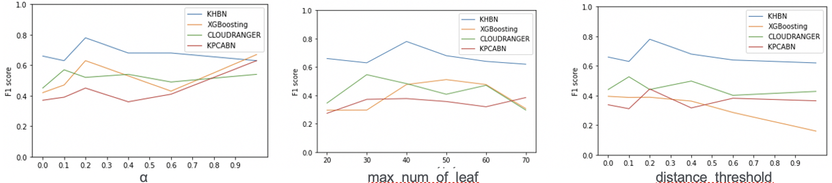
Figure 3. Parameter analysis

4.6. Computational Scalability

Based on the data size in Table 4 and number of nodes in Table 6, we have found that CloudRCA works efficiently in all the three platforms regardless of their different scale. To further demonstrate the scalability of CloudRCA, we evaluate the overheads of our method with synthetic data. We measured the run times of our method when trained with data of different size ranging from 50 to 1000, and different numbers of nodes for 50, 100, 300, 500 and 1000. The results in Table 11 indicate that the run time of KHBN linearly increases with the volume of training data and feature size thanks to the parallel computation and that KHBN consistently runs faster ($>50\%$) than the two graph-based competitors. In particular, with as many as 2000 samples and 1000 feature nodes, our workflow is able to finish model construction in 3.5 minutes, a much shorter time period than an SREs typically spends in manual troubleshooting.

Table 11. Overheads of the experiment

Production	Framework of RCA	50 nodes	100 nodes	300 nodes	500 nodes	1000 nodes
MaxCompute	KHBN	7.8s	17.4s	41.5s	102.3s	212.7s
	CLOUDRANGER	22.4s	51.2s	104.3s	251.8s	515.4s
	OM GRAPH	19.8s	52.3s	101.8s	247.5s	503.8s
RealtimeCompute	KHBN	6.9s	14.6s	37.7s	94.6s	195.8s
	CLOUDRANGER	19.6s	44.7s	95.3s	237.3s	503.7s
	OM GRAPH	20.5s	42.3s	98.7s	229.6s	495.6s
Hologres	KHBN	5.7s	11.2s	29.4s	91.8s	196.4s
	CLOUDRANGER	18.7s	37.8s	94.8s	228.4s	487.5s
	OM GRAPH	17.3s	36.1s	92.9s	215.7s	496.4s

4.7. Case Studies

CloudRCA workflow has been deployed in Alibaba’s three big data cloud computing platforms, MaxCompute, Realtime Compute and Hologres. The three platforms support the daily operations of Alibaba as well as the world-wide shopping festival “Double 11” with more than 100 thousand servers and complex architectures. The approach we proposed has helped SREs reduce the time of resolving a failure by more than $20\%$. When anomalies are detected in the Key Performance Indicators (KPIs) of a cloud computing platforms, SREs would receive a critical alarm together with the root cause type inferred by our RCA framework through dingtalk, an intelligent working platform created by Alibaba Group. By clicking the url in the alarm message, SREs are directed to an interface where all the important features are displayed. They can confirm those pre-defined automatic operations to remediate the system and provide feedback for the predicted root cause, and all these operations would be recorded and displayed on the interface. In the following, we share some real-world cases where CloudRCA greatly facilitates the identification of root causes when anomalies occur in the platforms.

Case 1: New types of root causes in MaxCompute. Due to the complex architecture and fast iteration of MaxCompute, it can be challenging for SREs to locate root cause types. The case is about a bug in the newly released version of the resource scheduler which prohibited some jobs from acquiring enough resources to finish on time. Since the root cause lied in the new version of the system, SREs had never seen this before and had no clues as to where to start troubleshooting. CloudRCA speeded up the procedure significantly by locating the root cause at the resource management module precisely, which helped SREs shrink the scope of debugging and save the time cost from up to 2 hours to a few minutes.

Case 2: Multiple anomalies in Realtime Compute. There was a fault related to a hotspot issue among the hosts of Realtime Compute. Since the hotspot affected the normal scheduler of jobs as well thus several KPIs in various modules became abnormal simultaneously, SREs got confused in locating the true underlying root cause. CloudRCA successfully identified the right root cause because it combines data from multiple sources, including not only KPIs but also logs of various modules. In this way, CloudRCA helped to reduce the time cost of troubleshooting by nearly 50%.

Case3: Hidden faults in Hologres. At the early development stage of Hologres, the KPIs in the monitoring systems were very limited. A batch of jobs running on Hologres encountered an unexpected failure, but none of the KPIs in the monitoring systems alarmed. Fortunately, CloudRCA not only detected the anomaly in log patterns but also provides the right root cause, since certain types of error logs kept increasing unexpectedly.

4.8. Cross-Platform Transfer Learning

Table 12. Performance for different modules before and after transfer learning

Production	Module	Precision before $\rightarrow$ after	Cover rate before $\rightarrow$ after	F1 before $\rightarrow$ after
MaxCompute	Resource Scheduler	86.3%	100%	0.93
	Storage	79.1% $\rightarrow$ 90.1%	66.7%	0.72 $\rightarrow$ 0.76
	Host	83.8% $\rightarrow$ 88.8%	60%	0.7 $\rightarrow$ 0.72
	Network	67.6% $\rightarrow$ 87.3%	100%	0.81 $\rightarrow$ 0.93
	Other	81.1%	75%	0.78
RealtimeCompute	Resource Scheduler	68.8%	100%	0.82
	Storage	85.7% $\rightarrow$ 92.9%	60% $\rightarrow$ 100%	0.71 $\rightarrow$ 0.96
	Host	78.9% $\rightarrow$ 84.2%	40% $\rightarrow$ 80%	0.53 $\rightarrow$ 0.82
	Network	66.7% $\rightarrow$ 75.0%	100%	0.8 $\rightarrow$ 0.86
	Other	78.9%	100%	0.88
Hologres	Resource Scheduler	54.5% $\rightarrow$ 68.8%	100%	0.71 $\rightarrow$ 0.82
	Storage	63.6% $\rightarrow$ 81.8%	60% $\rightarrow$ 100%	0.62 $\rightarrow$ 0.9
	Host	59.2% $\rightarrow$ 78.5%	60% $\rightarrow$ 80%	0.6 $\rightarrow$ 0.79
	Network	63.2% $\rightarrow$ 78.9%	66.7% $\rightarrow$ 100%	0.65 $\rightarrow$ 0.88
	Other	56.7%	100%	0.72

From the above experiments, we can see that models deployed on MaxCompute outperform Hologres significantly in almost every setup, since Hologres is a fairly new product with limited historical training data while MaxCompute is more mature. We notice that MaxCompute, Realtime Compute and Hologres share some common modules in their architecture as shown in Table 2, since they belong to Alibaba’s big data ecosystem and some modules may have the same KPIs. For example, although the three platforms run on different clusters, they share similar features on the Host and Network modules. As cloud has become an infrastructure with ever increasing popularity, more and more new systems are built on cloud, therefore a general mechanism to improve the root cause analysis performance in a relatively new cloud system can be beneficial. We designed a cross-platform transfer learning mechanism, which combines samples of the same modules from three different big data cloud computing platforms, so as to enrich the training set.

The experiment results are shown in Table 12, where we evaluate the performance of KHBN on each module separately. Numbers after the arrow show performance after applying the transfer learning mechanism. We can see that some common modules such as host, networks and storage benefit from transfer learning remarkably, while there is limited improvement in resource scheduler modules and storage module in Realtime Compute, since the techniques underlying these modules are relatively dependent. Another important trend is that cloud systems are developing its architecture toward could-native, and many cloud-native techniques such as Kubernetes has become a de facto standard, therefore transfer learning can be a promising approach to improve root cause analysis in relatively new cloud products.

4.9. Key Insights

We have the following key insights based on our comprehensive experiments: (1) Feature engineering lays the foundation for root cause inference in complex cloud systems by effectively extracting the most relevant information and shrinking the complexity of data, which eventually boosts both accuracy and efficiency in RCA. (2) Combining multiple sources of data provides RCA models with more comprehensive information to precisely locate root causes. (3) Predefined Knowledge and rich training data help improve the accuracy of RCA significantly. (4) Transfer learning across platforms can improve model accuracy when only limited training samples are available from relatively new cloud platforms, and can be a promising direction in cloud-native RCA.

5. Conclusion and Future Works

As Alibaba’s business keeps developing and flourishing, big data cloud computing platforms are faced with ever increasing challenges in providing stable and reliable service. In our study, we propose CloudRCA, a general framework including anomaly detection, log clustering and Bayesian network inference, to help detect anomalies and identify the root causes when systems fail. Comprehensive experiments have been done in our research to demonstrate the superiority, scalability and robustness of CloudRCA compared with other well-studied RCA frameworks. Moreover, CloudRCA has been deployed in Alibaba’s three typical cloud computing platforms including MaxCompute, Realtime Compute and Hologres and helps operators reduce the time of resolving a failure by more than 20% in the past 12 months. In addition, transfer learning across different platforms can improve the accuracy by more than 10% , which is promising for Alibaba’s big data ecosystem in the upcoming cloud native era. As a supplement and improvement, we’ll try GAN together with active learning in the future to reduce the cost of manual fault injection and labeling.

References

- (1)
- Ali et al. (2017) Mohd Rivaie Mohd Ali, Muhammad Imza Fakhri, Nujma Hayati, Nurul Atikah Ramli, and Ibrahim Jusoh. 2017. The n-th section method: A modification of Bisection. Malaysian Journal of Fundamental and Applied Sciences 13, 4 (2017), 728–731.
- Ester et al. (1996) Martin Ester, Hans-Peter Kriegel, Jörg Sander, Xiaowei Xu, et al. 1996. A density-based algorithm for discovering clusters in large spatial databases with noise.. In Kdd, Vol. 96. 226–231.
- Gower and Ross (1969) John C Gower and Gavin JS Ross. 1969. Minimum spanning trees and single linkage cluster analysis. Journal of the Royal Statistical Society: Series C (Applied Statistics) 18, 1 (1969), 54–64.
- Hochenbaum et al. (2017) Jordan Hochenbaum, Owen S Vallis, and Arun Kejariwal. 2017. Automatic anomaly detection in the cloud via statistical learning. arXiv preprint arXiv:1704.07706 (2017).
- Jia et al. (2017) Tong Jia, Lin Yang, Pengfei Chen, Ying Li, Fanjing Meng, and Jingmin Xu. 2017. Logsed: Anomaly diagnosis through mining time-weighted control flow graph in logs. In 2017 IEEE 10th International Conference on Cloud Computing (CLOUD). IEEE, 447–455.
- Leys et al. (2013) Christophe Leys, Christophe Ley, Olivier Klein, Philippe Bernard, and Laurent Licata. 2013. Detecting outliers: Do not use standard deviation around the mean, use absolute deviation around the median. Journal of experimental social psychology 49, 4 (2013), 764–766.
- Lin et al. (2016a) Jieyu Lin, Qi Zhang, Hadi Bannazadeh, and Alberto Leon-Garcia. 2016a. Automated anomaly detection and root cause analysis in virtualized cloud infrastructures. In NOMS 2016-2016 IEEE/IFIP Network Operations and Management Symposium. IEEE, 550–556.
- Lin et al. (2016b) Qingwei Lin, Hongyu Zhang, Jian-Guang Lou, Yu Zhang, and Xuewei Chen. 2016b. Log clustering based problem identification for online service systems. In 2016 IEEE/ACM 38th International Conference on Software Engineering Companion (ICSE-C). IEEE, 102–111.
- Liu et al. (2008) Fei Tony Liu, Kai Ming Ting, and Zhi-Hua Zhou. 2008. Isolation forest. In 2008 eighth ieee international conference on data mining. IEEE, 413–422.
- Marvasti et al. (2013) Mazda A Marvasti, Arnak V Poghosyan, Ashot N Harutyunyan, and Naira M Grigoryan. 2013. An anomaly event correlation engine: Identifying root causes, bottlenecks, and black swans in IT environments. VMware Technical Journal 2, 1 (2013), 35–45.
- Mikolov et al. (2013a) Tomas Mikolov, Kai Chen, Greg Corrado, and Jeffrey Dean. 2013a. Efficient estimation of word representations in vector space. arXiv preprint arXiv:1301.3781 (2013).
- Mikolov et al. (2013b) Tomas Mikolov, Ilya Sutskever, Kai Chen, Greg Corrado, and Jeffrey Dean. 2013b. Distributed representations of words and phrases and their compositionality. arXiv preprint arXiv:1310.4546 (2013).
- Qiu et al. (2020) Juan Qiu, Qingfeng Du, Kanglin Yin, Shuang-Li Zhang, and Chongshu Qian. 2020. A causality mining and knowledge graph based method of root cause diagnosis for performance anomaly in cloud applications. Applied Sciences 10, 6 (2020), 2166.
- Robert et al. (1990) Cleveland Robert, C William, and Terpenning Irma. 1990. STL: A seasonal-trend decomposition procedure based on loess. Journal of official statistics 6, 1 (1990), 3–73.
- Thalheim et al. (2017) Jörg Thalheim, Antonio Rodrigues, Istemi Ekin Akkus, Pramod Bhatotia, Ruichuan Chen, Bimal Viswanath, Lei Jiao, and Christof Fetzer. 2017. Sieve: Actionable insights from monitored metrics in distributed systems. In Proceedings of the 18th ACM/IFIP/USENIX Middleware Conference. 14–27.
- Wang et al. (2018) Ping Wang, Jingmin Xu, Meng Ma, Weilan Lin, Disheng Pan, Yuan Wang, and Pengfei Chen. 2018. Cloudranger: Root cause identification for cloud native systems. In 2018 18th IEEE/ACM International Symposium on Cluster, Cloud and Grid Computing (CCGRID). IEEE, 492–502.
- Wen et al. (2019) Qingsong Wen, Jingkun Gao, Xiaomin Song, Liang Sun, Huan Xu, and Shenghuo Zhu. 2019. RobustSTL: A robust seasonal-trend decomposition algorithm for long time series. In Proceedings of the AAAI Conference on Artificial Intelligence, Vol. 33. 5409–5416.
- Wen et al. (2021) Qingsong Wen, Kai He, Liang Sun, Yingying Zhang, Min Ke, and Huan Xu. 2021. RobustPeriod: Robust Time-Frequency Mining for Multiple Periodicity Detection. In Proceedings of the 2021 International Conference on Management of Data (SIGMOD). 2328–2337.
- Wen et al. (2020) Qingsong Wen, Zhe Zhang, Yan Li, and Liang Sun. 2020. Fast RobustSTL: Efficient and Robust Seasonal-Trend Decomposition for Time Series with Complex Patterns. In Proceedings of the 26th ACM SIGKDD International Conference on Knowledge Discovery & Data Mining (KDD). 2203–2213.
- Weng et al. (2018) Jianping Weng, Jessie Hui Wang, Jiahai Yang, and Yang Yang. 2018. Root cause analysis of anomalies of multitier services in public clouds. IEEE/ACM Transactions on Networking 26, 4 (2018), 1646–1659.
- Xu et al. (2017) Jingmin Xu, Pengfei Chen, Lin Yang, Fanjing Meng, and Ping Wang. 2017. Logdc: Problem diagnosis for declartively-deployed cloud applications with log. In 2017 IEEE 14th International Conference on e-Business Engineering (ICEBE). IEEE, 282–287.
- Yang et al. (2021) Linxiao Yang, Qingsong Wen, Bo Yang, and Liang Sun. 2021. A Robust and Efficient Multi-Scale Seasonal-Trend Decomposition. In ICASSP 2021-2021 IEEE International Conference on Acoustics, Speech and Signal Processing (ICASSP). IEEE, 5085–5089.
- Zeng et al. (2014) Chunqiu Zeng, Liang Tang, Tao Li, Larisa Shwartz, and Genady Ya Grabarnik. 2014. Mining temporal lag from fluctuating events for correlation and root cause analysis. In 10th International Conference on Network and Service Management (CNSM) and Workshop. IEEE, 19–27.
- Zhang et al. (2018) Shenglin Zhang, Ying Liu, Weibin Meng, Zhiling Luo, Jiahao Bu, Sen Yang, Peixian Liang, Dan Pei, Jun Xu, Yuzhi Zhang, et al. 2018. Prefix: Switch failure prediction in datacenter networks. Proceedings of the ACM on Measurement and Analysis of Computing Systems 2, 1 (2018), 1–29.
- Zoubir et al. (2012) Abdelhak M Zoubir, Visa Koivunen, Yacine Chakhchoukh, and Michael Muma. 2012. Robust estimation in signal processing: A tutorial-style treatment of fundamental concepts. IEEE Signal Processing Magazine 29, 4 (2012), 61–80.