Bogoliubov Fermi surfaces from pairing of emergent $j=3/2$ fermions
on the pyrochlore lattice

Abstract

We examine the appearance of superconductivity in the strong-coupling limit of the Hubbard model on the pyrochlore lattice. We focus upon the limit of half filling, where the normal-state band structure realizes a $j=3/2$ semimetal. Introducing doping, we show that the pairing is favored in a $J=2$ quintet $E_{g}$ state. The attractive interaction in this channel relies on the fact that $E_{g}$ pairing on the pyrochlore lattice avoids the detrimental on-site repulsion. Our calculations show that a time-reversal symmetry-breaking superconducting phase is favored, which displays Bogoliubov Fermi surfaces.

I Introduction

The physics of pyrochlore systems such as the iridate compounds $R_{2}$Ir₂O₇ ($R$ is a rare-earth element) has attracted much attention over the past decade [1, 2, 3, 4, 5, 6, 7, 8, 9, 10]. These materials are characterized by the interplay of strong electronic correlations and strong spin-orbit coupling [11], which is predicted to yield a variety of exotic correlated states, such as spin liquids [1] and magnetically-ordered states with nontrivial topology [2, 3, 4, 5, 6, 7, 8, 9, 10]. The pyrochlore crystal structure of these materials is characterized by a lattice of corner-sharing tetrahedra composed of Ir⁴⁺ ions, with the low-energy electronic states deriving from the spin-orbit-split $J_{\text{eff}}=1/2$ doublet of the $t_{2g}$ manifold of the Ir $5d$ orbitals [1]. Due to the cubic structure of the pyrochlore lattice, the low-energy Bloch states deriving from the $J_{\text{eff}}=1/2$ doublets of the four Ir ions in each unit cell can possess a nontrivial emergent $j=3/2$ angular momentum. This emergent angular momentum describes states near quadratic band-touchings at the Brillouin-zone center, which have been observed in a number of pyrochlore iridates [12, 13].

Fermionic systems with $j=3/2$ have been proposed to host a number of exotic ordered phases and possibly non-Fermi-liquid behavior [6, 14, 8]. In particular, the allowed superconducting states are much enriched: in addition to pairing in a spin-singlet ($J=0$) or triplet ($J=1$) channel, pairing in quintet ($J=2$) or septet ($J=3$) states is also allowed [15]. These higher spin states can display gap functions with remarkable nodal structures, e.g., Bogoliubov Fermi surfaces (BFSs) [16, 17, 18, 19, 20] or Dirac superconductors with quadratic or cubic nodal dispersions [21]. So far, however, these states have mostly been discussed in terms of the effective Luttinger model valid near the quadratic band-touching point [15, 22, 23, 24, 25], whereas theories of unconventional superconductors are more typically formulated in terms of tight-binding models with local interactions. Using the latter perspective, Laurell and Fiete [9] have studied superconductivity in a quasi-two-dimensional model of a pyrochlore lattice, but the breaking of cubic symmetry implies that the quasiparticles do not have $j=3/2$ character.

In this paper we motivate the pyrochlore lattice as a minimal tight-binding model in which to study the superconductivity of fermions with an emergent $j=3/2$ effective angular momentum. Including an on-site Hubbard repulsion $U$, we derive the pairing interaction in the strong-coupling limit. We find that the dominant pairing instability will be the extended s-wave $E_{g}$ pairing channel corresponding to $J=2$ quintet pairing, which is likely to realize a time-reversal-symmetry-breaking state with BFSs.

Our paper is organized as follows: In Sec. II, we introduce the tight-binding model of the pyrochlore lattice and determine the parameter regime where the $j=3/2$ fermionic quasiparticles are the low-energy excitations at half filling. The parameters of the effective Luttinger model are obtained in terms of the tight-binding parameters. In Sec. III.1, we postulate a general interaction Hamiltonian for our tight-binding model, including both on-site and nearest-neighbor interactions. We project this interaction onto the low-energy states and decouple it in the Cooper channel, restricting our attention to the states with nonzero pairing amplitude at the Brillouin-zone center, namely the singlet $A_{1g}$ state and the quintet $E_{g}$ and $T_{2g}$ states. Specializing to the strong-coupling limit, where the nearest-neighbor interaction potentials perturbatively arise from virtual hopping events, we argue in Sec. III.2 that the effective pairing interaction is repulsive in the $A_{1g}$ and $T_{2g}$ channels. In contrast, the pairing interaction is attractive in the $E_{g}$ channel, which we show in Sec. III.3 is generically realized in a time-reversal-symmetry-breaking state supporting BFSs.

II $j=3/2$ fermions on the pyrochlore lattice

The fundamental structural feature of the pyrochlore lattice are corner-sharing tetrahedra. The tetrahedra which do not directly touch one another form an fcc lattice. Taking the centers of these tetrahedra as the lattice points, the basis vectors for the four atoms are given by

$$\mathbf{b}_{1} =\frac{a}{4}\left(-\frac{1}{2},-\frac{1}{2},-\frac{1}{2}\right),$$ (1)

$$\mathbf{b}_{2} =\frac{a}{4}\left(\frac{1}{2},\frac{1}{2},-\frac{1}{2}\right),$$ (2)

$$\mathbf{b}_{3} =\frac{a}{4}\left(-\frac{1}{2},\frac{1}{2},\frac{1}{2}\right),$$ (3)

$$\mathbf{b}_{4} =\frac{a}{4}\left(\frac{1}{2},-\frac{1}{2},\frac{1}{2}\right),$$ (4)

where $a$ is the lattice constant of the conventional fcc unit cell.

The standard electronic model for the pyrochlore iridates is a tight-binding model extending up to next-nearest neighbors for Ir $J_{\text{eff}}=1/2$ doublets at each pyrochlore site [4]. For simplicity, henceforth we label these doublets by a spin degree of freedom $\{\uparrow,\downarrow\}$. The noninteracting model is described by the Hamiltonian

$$H= \sum_{\langle ij\rangle}c^{\dagger}_{i}\left(t_{1}+it_{2}{\bf d}_{ij}\cdot\bm{\sigma}\right)c_{j}$$

$$+\sum_{\langle\langle ij\rangle\rangle}c^{\dagger}_{i}\left(t^{\prime}_{1}+i\left[t_{2}^{\prime}{\bf R}_{ij}+t_{3}^{\prime}{\bf D}_{ij}\right]\cdot\bm{\sigma}\right)c_{j},$$ (5)

where $c_{i}=(c_{i,\uparrow},c_{i,\downarrow})^{T}$ is the spinor of creation and annihilation operators for the doublet states at site $i$, $\bm{\sigma}$ is the vector of Pauli matrices, and the vectors appearing in Eq. (II) are defined as [10]

$${\bf d}_{ij} =2{\bf b}_{i}\times{\bf b}_{j},$$ (6)

$${\bf R}_{ij} =({\bf b}_{i}-{\bf b}_{k})\times({\bf b}_{k}-{\bf b}_{j}),$$ (7)

$${\bf D}_{ij} ={\bf d}_{ik}\times{\bf d}_{kj},$$ (8)

where $k$ is a common nearest neighbor of sites $i$ and $j$. In the context of the iridates, the hopping integrals appearing in Eq. (II) can be expressed in terms of direct iridium-iridium hopping via $\sigma$ and $\pi$ bonds ($t_{\sigma}$, $t_{\pi}$, $t_{\sigma}^{\prime}$, $t_{\pi}^{\prime}$) and also indirect hopping via oxygen ions ($t_{O}$). The Slater-Koster method then predicts [4]

$$t_{1} =\frac{130}{243}\,t_{O}+\frac{17}{324}\,t_{\sigma}-\frac{79}{243}t_{\pi},$$ (9)

$$t_{2} =\frac{28}{243}\,t_{O}+\frac{15}{243}\,t_{\sigma}-\frac{40}{243}\,t_{\pi},$$ (10)

$$t_{1}^{\prime} =\frac{233}{2916}\,t_{\sigma}^{\prime}-\frac{407}{2187}\,t_{\pi}^{\prime},$$ (11)

$$t_{2}^{\prime} =\frac{1}{1458}\,t_{\sigma}^{\prime}+\frac{220}{2187}\,t_{\pi}^{\prime},$$ (12)

$$t_{3}^{\prime} =\frac{25}{1458}\,t_{\sigma}^{\prime}+\frac{460}{2187}\,t_{\pi}^{\prime}.$$ (13)

As mentioned in the introduction, the pyrochlore structure naturally gives rise to $j=3/2$ fermionic excitations. This is most easily understood by considering the electronic structure of an isolated tetrahedron with an Ir ion with a $J_{\text{eff}}=1/2$ doublet at each vertex. The orbital component of the electron wavefunctions for this four-site cluster can be decomposed into an s-wave-like ($A_{1}$ irrep of the point group $T_{d}$ of a tetrahedron) and three p-wave-like ($T_{2}$ irrep) wavefunctions. Spin-orbit coupling splits the electronic states of the isolated tetrahedron into two $j=1/2$ doublets and a $j=3/2$ quartet [26]. For the full pyrochlore lattice, this emergent electronic structure persists close to the $\Gamma$ point. In the following, we will focus on the case where the low-energy excitations are due only to the $j=3/2$ fermions. In particular, this is possible if the $j=3/2$ bands are half filled, in which case a semimetallic state with a quadratic band-touching point may be realized. This is of special interest as combining the half-filling condition with interactions raises the possibility of strongly-correlated $j=3/2$ fermions [27].

To quadratic order in momentum, the $j=3/2$ excitations close to the $\Gamma$ point are described by an effective Luttinger-Kohn model with Hamiltonian matrix

$$H_{\text{LK}}(\mathbf{k})=\alpha|\mathbf{k}|^{2}\hat{\mathbbm{1}}+\beta\sum_{\mu}k_{\mu}^{2}\hat{J}_{\mu}^{2}+\gamma\sum_{\mu\neq\nu}k_{\mu}k_{\nu}\hat{J}_{\mu}\hat{J}_{\nu},$$ (14)

where $\alpha$, $\beta$, and $\gamma$ are constants, $\hat{\mathbbm{1}}$ is the $4\times 4$ identity matrix, and $\hat{J}_{\mu}$, $\mu=x,y,z$, are the $j=3/2$ angular-momentum matrices; see Appendix A for a detailed derivation. The two distinct eigenvalues of the Luttinger-Kohn model are

$$E_{\pm,\mathbf{k}} =\left(\alpha+\frac{5}{4}\beta\right)|\mathbf{k}|^{2}$$

$$\quad{}\pm\sqrt{\beta^{2}\sum_{\mu}k_{\mu}^{4}+(3\gamma^{2}-\beta^{2})\sum_{\mu<\nu}k_{\mu}^{2}k_{\nu}^{2}}.$$ (15)

Both are twofold degenerate. By considering the dispersion along the $[100]$ and $[111]$ directions, the conditions for the bands to have opposite curvature, and thus for a semimetal, are

$$\mathop{\textrm{sgn}}\left[\left(\alpha+\frac{1}{4}\,\beta\right)\left(\alpha+\frac{9}{4}\,\beta\right)\right] =-1,$$ (16)

$$\mathop{\textrm{sgn}}\left[\left(\alpha+\frac{5}{4}\,\beta+|\gamma|\right)\left(\alpha+\frac{5}{4}\,\beta-|\gamma|\right)\right] =-1.$$ (17)

In Fig. 1(a), we plot the region in parameter space where these conditions are satisfied.

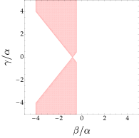
(a) (b)
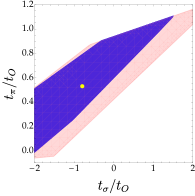
(c)

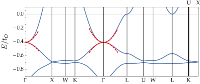
Figure 1: (Color online) (a) Range of parameters $\beta$ and $\gamma$ in the Luttinger-Kohn Hamiltonian where a $j=3/2$ semimetal is realized (shaded). (b) Range of parameters $t_{\sigma}$ and $t_{\pi}$ where a $j=3/2$ semimetal state is realized for the pyrochlore lattice: The pink (light gray) region indicates where a semimetallic quadratic band touching is found at the $\Gamma$ point and is obtained by mapping the region in panel (a) to the pyrochlore lattice using Eqs. (18)–(20). Within the enclosed dark blue (dark gray) region, there are no other states elsewhere in the Brillouin zone at the same energy as the quadratic band-touching point. (c) Typical band structure along high-symmetry directions showing the presence of a $j=3/2$ semimetal state. The parameter choice ($t_{\sigma}=-0.795t_{O}$, $t_{\pi}=0.53t_{O}$) is indicated by the yellow dot in panel (b). The dashed red lines show the low-energy bands in the equivalent Luttinger-Kohn model.

Projecting the pyrochlore Hamiltonian onto the $j=3/2$ subspace, we recover the Luttinger-Kohn model with the coefficients [8]

$$\alpha+\frac{5}{4}\,\beta =\frac{2}{3}\left(t_{1}+2t_{2}+6t_{1}^{\prime}-12t_{2}^{\prime}-12t_{3}^{\prime}\right),$$ (18)

$$\sqrt{3}\,\gamma =-\frac{2}{\sqrt{3}}\left(t_{1}+2t_{2}-2t_{1}^{\prime}-4t_{2}^{\prime}+12t_{3}^{\prime}\right),$$ (19)

$$\frac{\sqrt{3}}{2}\,\beta =-\frac{1}{\sqrt{3}}\left(t_{1}-t_{2}-6t_{1}^{\prime}-6t_{2}^{\prime}-6t_{3}^{\prime}\right).$$ (20)

The five distinct Slater-Koster hopping integrals would give a large parameter space to explore. However, we shall follow convention and set $t_{O}=1$ as our reference and then further impose that

$$t_{\sigma}^{\prime}=0.08\,t_{\sigma},\qquad t_{\pi}^{\prime}=0.08\,t_{\pi}.$$ (21)

Thus, we shall regard $t_{\sigma}$ and $t_{\pi}$ as free parameters. The parameter range in which the conditions Eqs. (16) and (17) for a semimetallic quadratic band touching are satisfied is shown by the pink region in Fig. 1(b). In this region, the $j=3/2$ states also lie between the two $j=1/2$ bands at the $\Gamma$ point, which is a necessary condition for such a semimetallic state at half filling. Since the Luttinger-Kohn Hamiltonian is only valid close to the $\Gamma$ point, however, it is possible that other states are present elsewhere in the Brillouin zone at the same energy as the quadratic band touching. Accounting for this shaves off some of the edges of the region identified by the conditions Eqs. (16) and (17), leaving the dark blue region in Fig. 1(b) as the parameter range where the low-energy excitations result solely from the quadratic band-touching point. Figure 1(c) shows a comparison of the tight-binding and Luttinger-Kohn model dispersions for the parameter values corresponding to the yellow dot in Fig. 1(b).

III Superconducting states

III.1 Pairing interactions

The most general interactions for spin-$1/2$ electrons consistent with the symmetry of the pyrochlore lattice up to nearest neighbors have the form [3, 9]

$$H_{\text{int}} =U_{0}\sum_{i}n_{i,\uparrow}n_{i,\downarrow}+U_{1}\sum_{\langle i,j\rangle}n_{i}n_{j}+J\sum_{\langle i,j\rangle}\mathbf{S}_{i}\cdot\mathbf{S}_{j}$$

$$\quad{}+D\sum_{\langle i,j\rangle}{\bf d}_{ij}\cdot(\mathbf{S}_{i}\times\mathbf{S}_{j})+\sum_{\langle i,j\rangle}\sum_{\mu,\nu}S^{\mu}_{i}\Gamma^{\mu\nu}_{ij}S^{\nu}_{j},$$ (22)

where $n_{i,\sigma}\equiv c_{i,\sigma}^{\dagger}c_{i,\sigma}$ is a number operator and $\mathbf{S}_{i}$ is a spin operator with components $S_{i}^{\mu}\equiv\sum_{\sigma,\sigma^{\prime}}c_{i,\sigma}^{\dagger}s^{\mu}_{\sigma\sigma^{\prime}}c_{i,\sigma^{\prime}}$, where $s^{\mu}=\sigma^{\mu}/2$ are the spin-$1/2$ matrices. The first line of Eq. (22) contains an on-site Hubbard repulsion as well as nearest-neighbor charge-charge and Heisenberg interactions. The second line contains the Dzyaloshinski-Moriya interaction and the traceless symmetric interaction

$$\Gamma^{\mu\nu}_{ij}=d^{\mu}_{ij}d^{\nu}_{ij}(\Gamma_{0}\delta_{\mu\nu}+\Gamma_{1}[1-\delta_{\mu\nu}]).$$ (23)

In performing the sum over nearest neighbors $\langle i,j\rangle$, we count each bond once.

The nearest-neighbor interactions in $H_{\text{int}}$ naturally arise in the strong-coupling limit of the Hubbard model [5, 9]. Ignoring next-nearest-neighbor hopping and assuming half filling and that the Hubbard energy $U_{0}$ greatly exceeds $t_{1}$ and $t_{2}$, we integrate out doubly occupied sites to obtain the effective interaction strengths

$$U_{1} =-\frac{2}{U_{0}}\,(t_{1}^{2}+2t_{2}^{2}),$$ (24)

$$J =\frac{4}{U_{0}}\left(t_{1}^{2}-\frac{2}{3}t_{2}^{2}\right),$$ (25)

$$D =\frac{8}{U_{0}}\,t_{1}t_{2},$$ (26)

$$\Gamma_{0} =\frac{8t_{2}^{2}}{3U_{0}},$$ (27)

$$\Gamma_{1} =-\frac{8t_{2}^{2}}{U_{0}}.$$ (28)

To work in the more convenient $j=3/2$ subspace, we project the interactions onto the low-energy states. We express the annihilation operator at site $a$ of tetrahedron $i$ in terms of the local operators in the $j=3/2$ subspace,

$$c_{i,a,\sigma}\approx\sum_{\alpha=-3/2}^{3/2}u_{a,\sigma;\alpha}\,c_{i,\alpha},$$ (29)

where the coefficients $u_{a,\sigma;\alpha}$ are obtained in Appendix A. Substituting Eq. (29) into Eq. (22), we obtain the effective interaction in the low-energy subspace,

$$H_{\text{int}} =\sum_{i}\sum_{\alpha,\alpha^{\prime}}\sum_{\beta,\beta^{\prime}}V_{\alpha\alpha^{\prime};\beta\beta^{\prime}}\,c^{\dagger}_{i,\alpha}c_{i,\alpha^{\prime}}c^{\dagger}_{i,\beta}c_{i,\beta^{\prime}}$$

$$\quad{}+\sum_{\langle i,j\rangle_{aa^{\prime}}}\sum_{\alpha,\alpha^{\prime}}\sum_{\beta,\beta^{\prime}}[V_{a,a^{\prime}}]_{\alpha\alpha^{\prime};\beta\beta^{\prime}}\,c^{\dagger}_{i,\alpha}c_{i,\alpha^{\prime}}c^{\dagger}_{j,\beta}c_{j,\beta^{\prime}},$$ (30)

where the sum over $\langle i,j\rangle_{aa^{\prime}}$ contains all nearest-neighbor pairs of sites $a$, $a^{\prime}$ on tetrahedra $i$, $j$. The interaction potentials are given by

$$V_{\alpha\alpha^{\prime};\beta\beta^{\prime}}=U_{0}\sum_{a}u_{a,\uparrow;\alpha}^{\ast}u_{a,\uparrow;\alpha^{\prime}}u_{a,\downarrow;\beta}^{\ast}u_{a,\downarrow;\beta^{\prime}}$$ (31)

for the on-site interaction and

$$[V_{a,a^{\prime}}]_{\alpha\alpha^{\prime};\beta\beta^{\prime}} =U_{1}\sum_{\sigma_{1},\sigma_{2}}u_{a,\sigma_{1};\alpha}^{\ast}u_{a,\sigma_{1};\alpha^{\prime}}u_{a^{\prime},\sigma_{2};\beta}^{\ast}u_{a^{\prime},\sigma_{2};\beta^{\prime}}$$

$$\quad{}+\sum_{\sigma_{1},\sigma_{2},\sigma_{3},\sigma_{4}}\sum_{\mu,\nu}s_{\sigma_{1}\sigma_{2}}^{\mu}s_{\sigma_{3}\sigma_{4}}^{\nu}$$

$$\qquad{}\times\Big{(}J\delta_{\mu\nu}+D\sum_{\rho}\epsilon^{\mu\nu\rho}d_{aa^{\prime}}^{\rho}+\Gamma^{\mu\nu}_{aa^{\prime}}\Big{)}$$

$$\qquad{}\times u_{a,\sigma_{1};\alpha}^{\ast}u_{a,\sigma_{2};\alpha^{\prime}}u_{a^{\prime},\sigma_{3};\beta}^{\ast}u_{a^{\prime},\sigma_{4};\beta^{\prime}}$$ (32)

for the nearest-neighbor interactions. Here, $\epsilon^{\mu\nu\rho}$ is the Levi-Civita symbol. The lengthy explicit expressions for the coefficients $u_{a,\sigma;\alpha}$ and the potentials $V$ and $V_{a,a^{\prime}}$ are relegated to Appendix B.

We treat $H_{\text{int}}$ in Eq. (30) as an effective pairing interaction, which we eventually want to decouple in the Cooper channel. To that end, we decompose the interaction into the even-parity Cooper channels, using the generalized Fierz identity [14]

$$(\psi^{\dagger}N\psi)(\phi^{\dagger}M\phi)=\sum_{\hat{A},\hat{B}}f_{NM}(\hat{A},\hat{B})\,(\psi^{\dagger}\bar{A}\phi^{\dagger T})(\phi^{T}\bar{B}^{\dagger}\psi),$$ (33)

where

$$f_{NM}(\hat{A},\hat{B})=\frac{1}{16}\,\mathop{\textrm{Tr}}(U_{T}^{\dagger}\hat{A}N\hat{B}U_{T}M^{T}).$$ (34)

The right-hand side of Eq. (33) represents a pairing interaction, where $\bar{A}\equiv\hat{A}U_{T}$ and $U_{T}=\exp(i\pi\hat{J}_{y})$ is the unitary part of the time-reversal operator. The matrices $\bar{A}$ describe the internal symmetry of the Cooper pairs in the $j=3/2$ space [17]. The six matrices compatible with even parity are listed in Table 1, together with the corresponding irreps. $\psi$ and $\phi$ are field operators on a basis of $j=3/2$ fermions.

Table 1: Internal symmetries of Cooper pairs allowed for even-parity pairing. The irreps of the point group $O_{h}$ and the pairing matrices are given. The matrix $U_{T}=\exp(i\pi\hat{J}_{y})$ is the unitary part of the time-reversal operator.

irrep	pairing state
$A_{1g}$	$\bar{\mathbbm{1}}=U_{T}$
$E_{g}$	$(\bar{E}_{1},\bar{E}_{2})=\frac{1}{\sqrt{3}}(\hat{J}_{x}^{2}-\hat{J}_{y}^{2},(2\hat{J}_{z}^{2}-\hat{J}_{x}^{2}-\hat{J}_{y}^{2})/\sqrt{3})\,U_{T}$
$T_{2g}$	$(\bar{T}_{1},\bar{T}_{2},\bar{T}_{3})=\frac{1}{\sqrt{3}}(\{\hat{J}_{y},\hat{J}_{z}\},\{\hat{J}_{z},\hat{J}_{x}\},\{\hat{J}_{x},\hat{J}_{y}\})\,U_{T}$

Transforming the interaction to momentum space and restricting ourselves to the pairing of electrons with opposite momenta, we write the pairing Hamiltonian as

$$H_{\text{pair}} =\frac{1}{2N}\sum_{\mathbf{k},\mathbf{k}^{\prime}}\sum_{\alpha,\beta,\alpha^{\prime},\beta^{\prime}}[V_{\mathbf{k},\mathbf{k}^{\prime}}]_{\alpha\beta;\alpha^{\prime}\beta^{\prime}}$$

$$\quad{}\times c^{\dagger}_{\mathbf{k},\alpha}c^{\dagger}_{-\mathbf{k},\beta}c_{{\bf-k^{\prime}},\alpha^{\prime}}c_{{\bf k^{\prime}},\beta^{\prime}},$$ (35)

where $N$ is the number of unit cells. The coupling strength contains contributions from the on-site interaction, Eq. (31), and from the nearest-neighbor interaction, Eq. (32). The undoped semimetal has the Fermi energy at the quadratic band-touching point and vanishing electronic density of states, and thus does not show superconductivity at weak coupling. Upon doping the semimetal, a small Fermi surface will appear at the zone center. We hence restrict our study to the even-parity channel since odd-parity superconductivity has a vanishing pairing amplitude at the $\Gamma$ point and is thus typically weak at this small Fermi surface.

The decomposition into the even-parity Cooper channels is performed in Appendix C. Here, we focus on the limit of weak doping, i.e., $k_{F}\ll\pi/a$. In this limit, only those terms that remain nonzero for $\mathbf{k}\to 0$ are important. The resulting pairing interaction then reads as

$$V_{\mathbf{k},\mathbf{k}^{\prime}} \approx\frac{U_{0}}{8}\,\bar{\mathbbm{1}}\mathbin{\bar{\otimes}}\bar{\mathbbm{1}}^{\prime}+\frac{U_{0}}{24}\,\vec{\bar{T}}\mathbin{\bar{\otimes}}\vec{\bar{T}}^{\prime}$$

$$\quad{}+\left(\frac{U_{1}}{18}-\frac{J}{216}-\frac{D}{27}-\frac{\Gamma_{0}}{108}+\frac{\Gamma_{1}}{54}\right)c_{A_{1g}}\mathbin{\bar{\otimes}}c_{A_{1g}}^{\prime}$$

$$\quad{}+\left(\frac{U_{1}}{9}-\frac{J}{108}+\frac{D}{27}-\frac{\Gamma_{0}}{54}-\frac{\Gamma_{1}}{54}\right)\vec{c}^{\,(E)}_{E_{g}}\mathbin{\bar{\otimes}}\vec{c}^{\,(E)\,\prime}_{E_{g}}$$

$$\quad{}+\left(\frac{5U_{1}}{54}+\frac{J}{216}-\frac{D}{27}+\frac{\Gamma_{0}}{108}+\frac{\Gamma_{1}}{54}\right)\vec{c}^{\,(T)}_{T_{2g}}\mathbin{\bar{\otimes}}\vec{c}^{\,(T)\,\prime}_{T_{2g}},$$ (36)

where we define the product $\mathbin{\bar{\otimes}}$ to simplify the notation such that for a given field operator $c_{\mathbf{k}}^{T}\equiv(c_{\mathbf{k},\frac{3}{2}},c_{\mathbf{k},\frac{1}{2}},c_{\mathbf{k},-\frac{1}{2}},c_{\mathbf{k},-\frac{3}{2}})$,

$$\sum_{\alpha,\beta,\alpha^{\prime},\beta^{\prime}}(\bar{A}\mathbin{\bar{\otimes}}\bar{B})_{\alpha\beta;\alpha^{\prime}\beta^{\prime}}\,c_{\mathbf{k},\alpha}^{\dagger}c_{-\mathbf{k},\beta}^{\dagger}c_{-\mathbf{k}^{\prime},\alpha^{\prime}}c_{\mathbf{k}^{\prime},\beta^{\prime}}$$

$$\qquad\equiv\sum_{\alpha,\beta,\alpha^{\prime},\beta^{\prime}}\bar{A}_{\alpha\beta}\bar{B}_{\beta^{\prime}\alpha^{\prime}}^{\ast}\,c_{\mathbf{k},\alpha}^{\dagger}c_{-\mathbf{k},\beta}^{\dagger}c_{-\mathbf{k}^{\prime},\alpha^{\prime}}c_{\mathbf{k}^{\prime},\beta^{\prime}}$$

$$\qquad=\left(\sum_{\alpha,\beta}c_{\mathbf{k},\alpha}^{\dagger}\bar{A}_{\alpha\beta}c_{-\mathbf{k},\beta}^{\dagger}\right)\left(\sum_{\alpha^{\prime},\beta^{\prime}}c_{-\mathbf{k}^{\prime},\alpha^{\prime}}\bar{B}_{\beta^{\prime}\alpha^{\prime}}^{\ast}c_{\mathbf{k}^{\prime},\beta^{\prime}}\right)$$

$$\qquad=(c_{\mathbf{k}}^{\dagger}\bar{A}c_{-\mathbf{k}}^{\dagger T})(c_{-\mathbf{k}^{\prime}}^{T}\bar{B}^{\dagger}c_{\mathbf{k}^{\prime}}).$$ (37)

The first line of Eq. (36) refers to on-site pairing, whereas the remaining terms result from nearest-neighbor interactions. The latter terms can be understood as extended s-wave pairing, and contain the matrix-valued functions

$$c_{A_{1g}} =(c_{x}c_{y}+c_{y}c_{z}+c_{z}c_{x})\,\bar{\mathbbm{1}},$$ (38)

$$\vec{c}_{E_{g}}^{\,(E)} =(c_{x}c_{y}+c_{y}c_{z}+c_{z}c_{x})\,\big{(}\bar{E}_{1},\bar{E}_{2}\big{)},$$ (39)

$$\vec{c}_{T_{2g}}^{\,(T)} =(c_{x}c_{y}+c_{y}c_{z}+c_{z}c_{x})\,\big{(}\bar{T}_{1},\bar{T}_{2},\bar{T}_{3}\big{)},$$ (40)

with $c_{\mu}=\cos k_{\mu}a$. The prime signifies dependence on $\mathbf{k}^{\prime}$. Full results are presented in Appendix C.

Equation (36) shows that on-site pairing in the $A_{1g}$ and $T_{2g}$ channels is penalized by the Hubbard interaction; in contrast, the on-site $E_{g}$ pairing is immune to the Hubbard repulsion $U_{0}$, and there is no on-site interaction in this channel. This is a key result of our work. The nearest-neighbor interactions in Eq. (22) lead to the momentum-dependent, extended s-wave pairing terms in Eq. (36). In the strong-coupling limit, the pairing potentials for extended s-wave pairing are

$$A_{1g}: \quad-\frac{1}{378}\,\frac{(7t_{1}+8t_{2})^{2}}{U_{0}}-\frac{121}{567}\,\frac{t_{2}^{2}}{U_{0}},$$ (41)

$$E_{g}: \quad-\frac{1}{189}\,\frac{(7t_{1}+4t_{2})^{2}}{U_{0}}-\frac{134}{567}\,\frac{t_{2}^{2}}{U_{0}},$$ (42)

$$T_{2g}: \quad-\frac{1}{486}\,\frac{(9t_{1}+8t_{2})^{2}}{U_{0}}-\frac{31}{243}\,\frac{t_{2}^{2}}{U_{0}}.$$ (43)

It is clear from this formulation that the interaction in the extended s-wave channels is always attractive.

III.2 $A_{1g}$ and $T_{2g}$ channels

Both the on-site and extended s-wave pairing potentials in the $A_{1g}$ and $T_{2g}$ channels are nonzero. The states will in general involve both components, e.g., in the case of the $A_{1g}$ irrep we have $\Delta_{A_{1g}}=\Delta_{o}\,\bar{\mathbbm{1}}+\Delta_{e}\,c_{A_{1g}}$. Following Ref. [28], the critical temperature of this mixed state is obtained from the solution of the determinantal equation

$$\det\begin{pmatrix}\chi_{oo}-\frac{1}{g_{o}}&\chi_{oe}\\ \chi_{oe}&\chi_{ee}-\frac{1}{g_{e}}\end{pmatrix}=0,$$ (44)

where $g_{o}$ and $g_{e}$ are the interactions for the on-site and extended s-wave channels, respectively, and the generalized superconducting susceptibilities are defined by

$$\chi_{ab}={\cal N}_{0}\int d\epsilon\,\frac{\tanh(\epsilon/k_{B}T)}{4\epsilon}\,\langle\mathop{\textrm{Tr}}(\hat{\Delta}_{a}{\cal P}\hat{\Delta}_{b}^{\dagger}{\cal P})\rangle_{\text{FS}},$$ (45)

where ${\cal N}_{0}$ is the density of states at the Fermi energy, and ${\cal P}$ projects onto the states at the Fermi surface.

The off-diagonal components in Eq. (44) account for the overlap between the on-site and extended s-wave states. Close to the Brillouin-zone center, the form factor of the extended s-wave states is

$$c_{x}c_{y}+c_{y}c_{z}+c_{z}c_{x}\cong{}3-|\mathbf{k}|^{2}a^{2}.$$ (46)

Assuming weak mass anisotropy of the quadratic bands, the extended s-wave potentials should open an approximately isotropic gap at the Fermi surface; the gap opened by the on-site potential is always isotropic. Accordingly, the response of the system to the on-site and the extended s-wave gaps will be very similar, and we expect the susceptibilities to be proportional, i.e., $\chi_{ee}\approx r^{2}\chi_{oo}$ and $\chi_{oe}\approx r\chi_{oo}$, where $r$ is the ratio of the gap opened by the extended to the on-site potential. The determinantal equation then reduces to

$$\chi_{oo}=\frac{1}{g_{o}+r^{2}g_{e}}.$$ (47)

For sufficiently large $U_{0}$, the on-site repulsion will dominate over the attractive extended s-wave pairing in Eqs. (41)–(43), and the effective coupling constant $g_{o}+r^{2}g_{e}$ will be repulsive. As such, we do not expect pairing in the $A_{1g}$ or $T_{2g}$ channels in the strong-coupling limit.

III.3 $E_{g}$ channels

We now turn our attention to the extended s-wave $E_{g}$ state. Since the $E_{g}$ pairing avoids the on-site Hubbard repulsion $U_{0}$, the interaction potential in this channel is always attractive, and it should be favored for sufficiently large $U_{0}$. In the following, we consider which $E_{g}$ pairing state is expected to be realized. The $E_{g}$ pairing channel being two dimensional, the properties of the superconducting state are determined by a two-component order parameter ${\Delta}_{E_{g}}\equiv(\Delta_{1},\Delta_{2})$. A general Landau free-energy expansion in terms of these parameters suggests three possible ground states: $(1,0)$, $(0,1)$, and $(1,i)$ [15, 29]. The free energies of the $(1,0)$ and $(0,1)$ states are not expected to be the same as the two states are not related by any point-group operation [17, 22]. The third state breaks TRS due to the imaginary number $i$ and thus has BFSs beyond infinitesimal coupling strength [16, 17].

Within the BCS formalism, the mean-field-decoupled pairing interaction in the $E_{g}$ channel takes the form

$$H_{\mathrm{pair}}^{\mathrm{BCS}}=\frac{1}{2N}\sum_{\mathbf{k},\mathbf{k}^{\prime}}\sum_{m=1}^{2}\bigg{[}\Delta_{m}(\mathbf{k})f(\mathbf{k}^{\prime})\,c_{\mathbf{k}^{\prime}}^{\dagger}\bar{E}_{m}c_{-\mathbf{k}^{\prime}}^{\dagger T}$$

$$\quad{}+\Delta_{m}^{*}(\mathbf{k^{\prime}})f(\mathbf{k})\,c_{-\mathbf{k}}^{T}\bar{E}_{m}^{\dagger}c_{\mathbf{k}}+\frac{\Delta_{m}(\mathbf{k})\Delta_{m}^{*}(\mathbf{k^{\prime}})}{V_{0}}\bigg{]},$$ (48)

with the two components of the two-dimensional $E_{g}$ order parameter

$$\Delta_{1,2}(\mathbf{k})=-V_{0}f(\mathbf{k})\,\langle c_{-\mathbf{k}}^{T}\bar{E}_{1,2}^{\dagger}c_{\mathbf{k}}\rangle.$$ (49)

Here, $f(\mathbf{k})=c_{x}c_{y}+c_{y}c_{z}+c_{z}c_{x}$ is the extended s-wave form factor, $V_{0}$ is the absolute value of the interaction strength given by Eq. (42), and $\bar{E}_{1,2}$ are the pairing matrices in the $E_{g}$ channel of $j=3/2$ fermions, see Table 1 and Eqs. (77)–(79) in Appendix A.

To study superconductivity, we numerically solve the gap equation at $T=0$,

$$\Delta_{m}=\frac{V_{0}}{2N}\sum_{\mathbf{k},i\,\in\,\mathrm{occ}}\frac{\partial|E_{\mathbf{k},i}|}{\partial\Delta_{m}},$$ (50)

where $\Delta_{m}=N^{-1}\sum_{\mathbf{k}}\Delta_{m}(\mathbf{k})$, $m=1,2$, $i$ represents the band index, and the sum is over all occupied states, i.e., all states with $E_{\mathbf{k},i}<0$. The derivatives can be calculated in analytical form since the problem of finding the quasiparticle energies $E_{\mathbf{k},i}$ reduces to the solution of a quartic equation. Details of the numerical method are relegated to Appendix D.

The free energy per unit cell at $T=0$, i.e., the internal energy per unit cell, reads as

$$F=-\frac{1}{N}\sum_{\mathbf{k},i\,\in\,\mathrm{occ}}|E_{\mathbf{k},i}|+\sum_{m=1}^{2}\frac{|\Delta_{m}|^{2}}{V_{0}}.$$ (51)

We compare the free energies for the three pairing states and plot the free-energy gain, i.e., the condensation energy, on a logarithmic scale as a function of $V_{0}$ and of $U_{0}$ in Fig. 2. For weak interactions $V_{0}$ and thus small gap, the energy gain is maximal for the TRS-broken $(1,i)$ state. Increasing $V_{0}$, a first-order transition occurs to the TRS-preserving $(0,1)$ state.

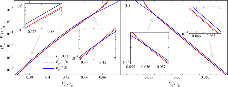
Figure 2: Condensation energy $F_{n}-F_{s}$ per unit cell for the three $E_{g}$ pairing states as a function of (a) the interaction strength $V_{0}$ and (b) the Hubbard repulsion $U_{0}$. The insets show close-ups of regimes with weak and strong interaction. Note that the energetically preferred state corresponds to the largest value. Here, parameters $t_{1}=0.321$, $t_{2}=-0.021$, $t_{1}^{\prime}=-0.013$, $t_{2}^{\prime}=0.004$, $t_{3}^{\prime}=0.008$ are used in the numerical calculation. This corresponds to the band structure presented in Fig. 1.

We can understand this result as follows: from Sigrist and Ueda [29], $(1,i)$ is expected to be the most stable state in the weak-coupling limit since it has point nodes and thus lower density of states close to the Fermi energy than the $(1,0)$ and $(0,1)$ states with line nodes. For strong pairing interactions, however, the $(1,i)$ state develops large BFSs, which lead to large density of states (DOS) and is thus no longer expected to be favored. The TRS-preserving $(0,1)$ state is found to be more stable than the also TRS-preserving $(1,0)$ state. They both have two line nodes but for the $(1,0)$ state these nodes cross each other, whereas for $(0,1)$ they do not. The crossing leads to higher DOS at the Fermi energy and is thus disfavored [29].

In Fig. 2(a), the data for small $V_{0}$ also show the expected weak-coupling behavior $F_{n}-F_{s}\sim e^{-A/V_{0}}$ at $T=0$ with some constant $A$; see also Appendix D. It is thus safe to extrapolate this curve down to zero interaction, which is not done here, though. In Fig. 2(b), the energy gain vs. the Hubbard repulsion $U_{0}$ shows nearly linear behavior, which follows from the fact that $\log(F_{n}-F_{s})$ is linear in $1/V_{0}$ in weak-coupling BCS theory and that $V_{0}$ is inversely proportional to $U_{0}$; see Eq. (42). The energies in Fig. 2 are given in units of $t_{O}$. To estimate the absolute energy scale, we note that the band width of the four bands in the model is roughly $2.5\,t_{O}$. Recent band-structure calculations for various pyrochlore iridates by Antonov et al. [30] predict band widths of about $600\,\mathrm{meV}$ to $800\,\mathrm{meV}$. This yields $t_{O}\approx 300\,\mathrm{meV}$. Using this value, we find that the condensation energy in Fig. 2 is comparable to that predicted by weak-coupling BCS theory in elemental superconductors.

The differences in condensation energy of the various pairing states in Fig. 2 look rather small. This is in fact a misleading impression of the logarithmic plot. The relevant energy scale is the condensation energy itself. In Fig. 3, we therefore plot the ratio of $\Delta F\equiv F_{n}-F_{s}$ for the $(0,1)$, $(1,0)$, and $(1,i)$ states to $\Delta F$ for the $(1,i)$ state, which is favored over much of the considered range of $V_{0}$. Evidently, the energetic separation between the three states is sizable on the relevant energy scale.

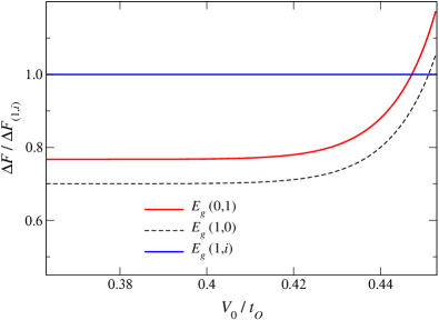
Figure 3: Ratios of the condensation energies $\Delta F\equiv F_{n}-F_{s}$ for the $E_{g}$ pairing states $(0,1)$, $(1,0)$, and $(1,i)$ to the condensation energy $\Delta F_{(1,i)}$ for the $(1,i)$ state. The parameters are the same as in Fig. 2.

IV Conclusions

In this work we have proposed the Hubbard model on the pyrochlore lattice as a minimal tight-binding model in which to study the superconductivity of emergent $j=3/2$ fermions. In particular, we have demonstrated that doping the strong-coupling limit of the half-filled Hubbard model on the pyrochlore lattice generates an attractive interaction in the extended s-wave quintet $E_{g}$ channel. This attractive interaction results solely from the Hubbard repulsion. The main point here is that pairing in the $E_{g}$ channel avoids a local repulsive interaction and so is driven by non-local attractive magnetic interactions. For sufficiently strong on-site interaction, the $E_{g}$ pairing channel will be favored over competing states in the $A_{1g}$ and $T_{2g}$ channels. Our numerical calculation shows that this $E_{g}$ pairing state likely breaks time-reversal symmetry, and hence will support BFSs. The time-reversal-symmetry-breaking state is compatible with the $d+id$ state found for a quasi-two-dimensional model [9].

Our analysis has focused entirely on pairing in the low-energy $j=3/2$ states, which emerge from the characteristic tetrahedral structural elements of the pyrochlore lattice. However, close to the boundaries of the $j=3/2$ semimetal phase shown in Fig. 1(b), doping the pyrochlore lattice will typically produce Fermi pockets of other bands elsewhere in the Brillouin zone. Since these states do not generally have $j=3/2$ character, care must be taken in considering the significance of the pairing interaction in these regions. In particular, the condition that the gap be nonzero at the zone center is less relevant, and the restriction to s-wave-like states is no longer justified. Hence, it is promising to search for metallic pyrochlores with small Fermi pockets around the $\Gamma$ point.

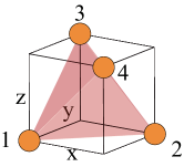
Figure 4: Positions of sublattice $a=1,2,3,4$ in the elementary tetrahedron.

Appendix A Derivation of Luttinger-Kohn Hamiltonian

In this appendix, we review the derivation of the Luttinger-Kohn Hamiltonian from the pyrochlore lattice [8]. The Hamiltonian is obtained by projecting out the $j=1/2$ subspaces and then expanding up to the quadratic order in momentum. To this end, we first provide the momentum-space form of the Hamiltonian $H=\sum_{a,a^{\prime}}\sum_{\sigma\sigma^{\prime}}\sum_{\mathbf{k}}c_{a,\sigma,\mathbf{k}}^{\dagger}[\hat{H}_{0}(\mathbf{k})+\hat{H}_{\rm SO}(\mathbf{k})]_{a,\sigma;a^{\prime},\sigma^{\prime}}c_{a^{\prime},\sigma^{\prime},\mathbf{k}}$ with

$$\hat{H}_{0}(\mathbf{k}) =F_{xy}^{+}\sigma_{0}\otimes\hat{\lambda}_{1}+F_{yz}^{+}\sigma_{0}\otimes\hat{\lambda}_{4}+F_{zx}^{+}\sigma_{0}\otimes\hat{\lambda}_{9}$$

$$\quad{}+F_{zx}^{-}\sigma_{0}\otimes\hat{\lambda}_{6}+F_{yz}^{-}\sigma_{0}\otimes\hat{\lambda}_{11}+F_{xy}^{-}\sigma_{0}\otimes\hat{\lambda}_{13}$$ (52)

and

$$\hat{H}_{\rm SO}(\mathbf{k}) =(G_{xy}^{+}\sigma_{x}-G_{xy}^{+}\sigma_{y}+K_{xy}^{-}\sigma_{z})\otimes\hat{\lambda}_{2}$$

$$\quad{}+(G_{yz}^{+}\sigma_{y}-G_{yz}^{+}\sigma_{z}+K_{yz}^{-}\sigma_{x})\otimes\hat{\lambda}_{5}$$

$$\quad{}+(G_{zx}^{+}\sigma_{z}-G_{zx}^{+}\sigma_{x}+K_{zx}^{-}\sigma_{y})\otimes\hat{\lambda}_{10}$$

$$\quad{}+(G_{zx}^{-}\sigma_{z}+G_{zx}^{-}\sigma_{x}+K_{zx}^{+}\sigma_{y})\otimes\hat{\lambda}_{7}$$

$$\quad{}-(G_{yz}^{-}\sigma_{y}+G_{yz}^{-}\sigma_{z}+K_{yz}^{+}\sigma_{x})\otimes\hat{\lambda}_{12}$$

$$\quad{}+(G_{xy}^{-}\sigma_{x}+G_{xy}^{-}\sigma_{y}+K_{xy}^{+}\sigma_{z})\otimes\hat{\lambda}_{14},$$ (53)

where $c_{a,\sigma,\mathbf{k}}$ is a fermion annihilation operator for sublattice $a=1,2,3,4$, see Fig. 4, and spin $\sigma={\uparrow},\downarrow$. The momentum dependence is represented by functions $F_{ij}^{\pm}$, $G_{ij}^{\pm}$, and $K_{ij}^{\pm}$ such that

$$F_{ij}^{\pm} =2t_{1}\cos(k_{i}\pm k_{j})+4t_{1}^{\prime}\cos(2k_{l})\cos(k_{i}\mp k_{j}),$$ (54)

$$G_{ij}^{\pm} =-2t_{2}\cos(k_{i}\pm k_{j})$$

$$\quad{}+4(t_{2}^{\prime}+t_{3}^{\prime})\cos(2k_{l})\cos(k_{i}\mp k_{j}),$$ (55)

$$K_{ij}^{\pm} =4(t_{2}^{\prime}-t_{3}^{\prime})\cos(2k_{l})\sin(k_{i}\mp k_{j}),$$ (56)

where $l\in\{x,y,z\}\setminus\{i,j\}$ and the lattice constant has been set to $a=4$. $\sigma_{0}$ is the $2\times 2$ identity matrix, $\sigma_{i}$ are the Pauli matrices, and $\hat{\lambda}_{j}$ are the $\mathrm{SU}(4)$ generators

$$\hat{\lambda}_{1} =\begin{pmatrix}0&1&0&0\\ 1&0&0&0\\ 0&0&0&0\\ 0&0&0&0\end{pmatrix}, \hat{\lambda}_{2} =\begin{pmatrix}0&-i&0&0\\ i&0&0&0\\ 0&0&0&0\\ 0&0&0&0\end{pmatrix},$$ (57)

$$\hat{\lambda}_{3} =\begin{pmatrix}1&0&0&0\\ 0&-1&0&0\\ 0&0&0&0\\ 0&0&0&0\end{pmatrix}, \hat{\lambda}_{4} =\begin{pmatrix}0&0&1&0\\ 0&0&0&0\\ 1&0&0&0\\ 0&0&0&0\end{pmatrix},$$ (58)

$$\hat{\lambda}_{5} =\begin{pmatrix}0&0&-i&0\\ 0&0&0&0\\ i&0&0&0\\ 0&0&0&0\end{pmatrix}, \hat{\lambda}_{6} =\begin{pmatrix}0&0&0&0\\ 0&0&1&0\\ 0&1&0&0\\ 0&0&0&0\end{pmatrix},$$ (59)

$$\hat{\lambda}_{7} =\begin{pmatrix}0&0&0&0\\ 0&0&-i&0\\ 0&i&0&0\\ 0&0&0&0\end{pmatrix}, \hat{\lambda}_{8} =\frac{1}{\sqrt{3}}\begin{pmatrix}1&0&0&0\\ 0&1&0&0\\ 0&0&-2&0\\ 0&0&0&0\end{pmatrix},$$ (60)

$$\hat{\lambda}_{9} =\begin{pmatrix}0&0&0&1\\ 0&0&0&0\\ 0&0&0&0\\ 1&0&0&0\end{pmatrix}, \hat{\lambda}_{10} =\begin{pmatrix}0&0&0&-i\\ 0&0&0&0\\ 0&0&0&0\\ i&0&0&0\end{pmatrix},$$ (61)

$$\hat{\lambda}_{11} =\begin{pmatrix}0&0&0&0\\ 0&0&0&1\\ 0&0&0&0\\ 0&1&0&0\end{pmatrix}, \hat{\lambda}_{12} =\begin{pmatrix}0&0&0&0\\ 0&0&0&-i\\ 0&0&0&0\\ 0&i&0&0\end{pmatrix},$$ (62)

$$\hat{\lambda}_{13} =\begin{pmatrix}0&0&0&0\\ 0&0&0&0\\ 0&0&0&1\\ 0&0&1&0\end{pmatrix}, \hat{\lambda}_{14} =\begin{pmatrix}0&0&0&0\\ 0&0&0&0\\ 0&0&0&-i\\ 0&0&i&0\end{pmatrix},$$ (63)

$$\hat{\lambda}_{15} =\frac{1}{\sqrt{6}}\begin{pmatrix}1&0&0&0\\ 0&1&0&0\\ 0&0&1&0\\ 0&0&0&-3\end{pmatrix}.$$ (64)

We first examine the band degeneracy at the $\Gamma$ point. In the absence of spin-orbit coupling ($t_{2}=t_{2}^{\prime}=t_{3}^{\prime}=0$), the eight bands split into sixfold and twofold degenerate bands. This can be seen by diagonalizing $\mathcal{H}_{0}(\mathbf{k})$ through the unitary transformation

$$S_{1}^{\dagger}\hat{H}_{0}({\bf 0})S_{1}=-2(t_{1}+2t_{1}^{\prime})\sqrt{6}\;\sigma_{0}\otimes\hat{\lambda}_{15},$$ (65)

with

$$S_{1}=\frac{1}{2}\,\sigma_{0}\otimes\begin{pmatrix}1&-1&1&-1\\ -1&1&1&-1\\ 1&1&-1&-1\\ -1&-1&-1&-1\end{pmatrix}.$$ (66)

When the spin-orbit couplings are turned on, the sixfold degeneracy further splits into twofold and fourfold degenerate bands:

$$S_{2}^{\dagger} S_{1}^{\dagger}[\mathcal{H}_{0}({\bf 0})+\mathcal{H}_{\rm SO}({\bf 0})]S_{1}S_{2}$$

$$=-2(t_{1}+2t_{1}^{\prime})\sqrt{6}\;\sigma_{0}\otimes\hat{\lambda}_{15}$$

$$\quad{}-4[t_{2}-2(t_{2}^{\prime}+t_{3}^{\prime})]\sqrt{3}\;\sigma_{0}\otimes\hat{\lambda}_{8},$$ (67)

under the unitary transformation with

$$S_{2}=\begin{pmatrix}\frac{i}{2}&\frac{i}{2}&\frac{1}{2\sqrt{3}}&-\frac{1}{2\sqrt{3}}&0&-\frac{1}{\sqrt{3}}&0&0\\ -\frac{1}{2\sqrt{3}}&\frac{1}{2\sqrt{3}}&-\frac{i}{2}&-\frac{i}{2}&\frac{1}{\sqrt{3}}&0&0&0\\ \frac{1}{2}&\frac{1}{2}&\frac{i}{2\sqrt{3}}&-\frac{i}{2\sqrt{3}}&0&-\frac{i}{\sqrt{3}}&0&0\\ \frac{i}{2\sqrt{3}}&-\frac{i}{2\sqrt{3}}&\frac{1}{2}&\frac{1}{2}&-\frac{i}{\sqrt{3}}&0&0&0\\ \frac{1}{\sqrt{3}}&-\frac{1}{\sqrt{3}}&0&0&\frac{1}{\sqrt{3}}&0&0&0\\ 0&0&\frac{1}{\sqrt{3}}&-\frac{1}{\sqrt{3}}&0&\frac{1}{\sqrt{3}}&0&0\\ 0&0&0&0&0&0&1&0\\ 0&0&0&0&0&0&0&1\end{pmatrix}.$$ (68)

As a result, the eight energy bands are split into a $j=3/2$ quartet and two $j=1/2$ doublets. Since we are interested in the $j=3/2$ quartet, we hereafter project the Hamiltonian onto the $j=3/2$ subspace and discard the $j=1/2$ doublets. The dispersion relation around the $\Gamma$ point can be obtained by expanding the projected Hamiltonian up to the quadratic order in momentum. Applying yet another unitary transformation with

$$S_{3}=\frac{1}{2}\begin{pmatrix}1-i&-1-i&0&0\\ 1-i&1+i&0&0\\ 0&0&-1-i&1-i\\ 0&0&1+i&1-i\end{pmatrix}$$ (69)

to the projected Hamiltonian results in a Luttinger-Kohn Hamiltonian of the canonical form

$$\hat{H}_{\rm LK}(\mathbf{k}) =\left(E_{0}+\alpha^{\prime}|\mathbf{k}|^{2}\right)\mathbbm{1}_{4\times 4}$$

$$\quad{}+\beta^{\prime}\left(\sqrt{3}k_{y}k_{z}\hat{\Gamma}_{1}+\sqrt{3}k_{z}k_{x}\hat{\Gamma}_{2}+\sqrt{3}k_{x}k_{y}\hat{\Gamma}_{3}\right)$$

$$\quad{}+\gamma^{\prime}\left[\frac{\sqrt{3}(k_{x}^{2}-k_{y}^{2})}{2}\,\hat{\Gamma}_{4}+\frac{(2k_{z}^{2}-k_{x}^{2}-k_{y}^{2})}{2}\,\hat{\Gamma}_{5}\right],$$ (70)

with

$$E_{0} =-2\left[t_{1}+2(t_{2}+t_{1}^{\prime})-4(t_{2}^{\prime}+t_{3}^{\prime})\right],$$ (71)

$$\alpha^{\prime} =\frac{2}{3}\,[t_{1}+2t_{2}+6t_{1}^{\prime}-12(t_{2}^{\prime}+t_{3}^{\prime})],$$ (72)

$$\beta^{\prime} =-\frac{2}{3}\left[t_{1}+2(t_{2}-t_{1}^{\prime}-2t_{2}^{\prime}+6t_{3}^{\prime})\right],$$ (73)

$$\gamma^{\prime} =-\frac{2}{3}\,[t_{1}-t_{2}-6(t_{1}^{\prime}+t_{2}^{\prime}+t_{3}^{\prime})].$$ (74)

Five mutually anticommuting $\Gamma$ matrices are defined as

$$\hat{\Gamma}_{1} =\frac{1}{\sqrt{3}}\,\{\hat{J}_{y},\hat{J}_{z}\},\hat{\Gamma}_{2}=\frac{1}{\sqrt{3}}\,\{\hat{J}_{z},\hat{J}_{x}\},\hat{\Gamma}_{3}=\frac{1}{\sqrt{3}}\,\{\hat{J}_{x},\hat{J}_{y}\},$$ (75)

$$\hat{\Gamma}_{4} =\frac{\hat{J}_{x}^{2}-\hat{J}_{y}^{2}}{\sqrt{3}},\hat{\Gamma}_{5}=\frac{2\hat{J}_{z}^{2}-\hat{J}_{x}^{2}-\hat{J}_{y}^{2}}{3},$$ (76)

where the $\hat{J}_{\mu}$ are the spin-$3/2$ matrices

$$\hat{J}_{x} =\frac{1}{2}\begin{pmatrix}0&\sqrt{3}&0&0\\ \sqrt{3}&0&2&0\\ 0&2&0&\sqrt{3}\\ 0&0&\sqrt{3}&0\end{pmatrix},$$ (77)

$$\hat{J}_{y} =\frac{i}{2}\begin{pmatrix}0&-\sqrt{3}&0&0\\ \sqrt{3}&0&-2&0\\ 0&2&0&-\sqrt{3}\\ 0&0&\sqrt{3}&0\end{pmatrix},$$ (78)

$$\hat{J}_{z} =\frac{1}{2}\begin{pmatrix}3&0&0&0\\ 0&1&0&0\\ 0&0&-1&0\\ 0&0&0&-3\end{pmatrix}.$$ (79)

Comparing Eq. (70) with Eq. (14), we obtain the relationship between the coefficients in the two Hamiltonians,

$$\alpha^{\prime}=\left(\alpha+\frac{5}{4}\,\beta\right),\quad\beta^{\prime}=\gamma,\quad\gamma^{\prime}=\beta.$$ (80)

From the elements of the full unitary transformation matrix $S_{1}S_{2}S_{3}$, we can express the projection of the annihilation operators in the site-spin basis onto the low-energy $j=3/2$ subspace at the Brillouin zone center:

$$c_{{\bf 0},1,\uparrow} =\frac{i}{2}\,c_{{\bf 0},{3}/{2}}-\frac{1+i}{2\sqrt{3}}\,c_{{\bf 0},{1}/{2}}-\frac{1}{2\sqrt{3}}\,c_{{\bf 0},-{1}/{2}},$$ (81)

$$c_{{\bf 0},1,\downarrow} =\frac{i}{2\sqrt{3}}\,c_{{\bf 0},{1}/{2}}-\frac{1+i}{2\sqrt{3}}\,c_{{\bf 0},-{1}/{2}}-\frac{1}{2}\,c_{{\bf 0},-{3}/{2}},$$ (82)

$$c_{{\bf 0},2,\uparrow} =-\frac{i}{2}\,c_{{\bf 0},{3}/{2}}-\frac{1+i}{2\sqrt{3}}\,c_{{\bf 0},{1}/{2}}+\frac{1}{2\sqrt{3}}\,c_{{\bf 0},-{1}/{2}},$$ (83)

$$c_{{\bf 0},2,\downarrow} =-\frac{i}{2\sqrt{3}}\,c_{{\bf 0},{1}/{2}}-\frac{1+i}{2\sqrt{3}}\,c_{{\bf 0},-{1}/{2}}+\frac{1}{2}\,c_{{\bf 0},-{3}/{2}},$$ (84)

$$c_{{\bf 0},3,\uparrow} =\frac{1}{2}\,c_{{\bf 0},{3}/{2}}+\frac{1+i}{2\sqrt{3}}\,c_{{\bf 0},{1}/{2}}-\frac{i}{2\sqrt{3}}\,c_{{\bf 0},-{1}/{2}},$$ (85)

$$c_{{\bf 0},3,\downarrow} =\frac{1}{2\sqrt{3}}\,c_{{\bf 0},{1}/{2}}+\frac{1+i}{2\sqrt{3}}\,c_{{\bf 0},-{1}/{2}}-\frac{i}{2}\,c_{{\bf 0},-{3}/{2}},$$ (86)

$$c_{{\bf 0},4,\uparrow} =-\frac{1}{2}\,c_{{\bf 0},{3}/{2}}+\frac{1+i}{2\sqrt{3}}\,c_{{\bf 0},{1}/{2}}+\frac{i}{2\sqrt{3}}\,c_{{\bf 0},-{1}/{2}},$$ (87)

$$c_{{\bf 0},4,\downarrow} =-\frac{1}{2\sqrt{3}}\,c_{{\bf 0},{1}/{2}}+\frac{1+i}{2\sqrt{3}}\,c_{{\bf 0},-{1}/{2}}+\frac{i}{2}\,c_{{\bf 0},-{3}/{2}},$$ (88)

where $c_{{\bf k},n,\sigma}$ annihilates an electron with momentum ${\bf k}$ and spin $\sigma$ at site $n$ of the tetrahedron, and $c_{{\bf k},\tilde{s}}$ annihilates an electron with momentum ${\bf k}$ and $\tilde{s}=-3/2,-1/2,1/2,3/2$. Although the coefficients in Eqs. (81)–(88) will be momentum-dependent away from ${\bf k}={\bf 0}$, we continue to use the ${\bf k}={\bf 0}$ coefficients since the $j=3/2$ description is only valid sufficiently close to the Brillouin-zone center, where the zero-order contributions to these coefficients dominate. Within this approximation, it follows that the coefficients $u_{a,\sigma,j}$ in Eq. (29) are identical to the coefficients appearing in Eqs. (81)–(88).

Appendix B Interactions projected onto the $j=3/2$ subspace

In this appendix, we derive the explicit form of the on-site and nearest-neighbor interactions $V$ and $V_{a,a^{\prime}}$ projected onto the $j=3/2$ subspace. These are obtained by substituting Eqs. (81)–(88) into Eqs. (31) and (32). To obtain a compact description, we employ a symmetric form presented in Ref. 14. A local interaction term can be written as

$$g_{NM}(\psi^{\dagger}N\psi)(\phi^{\dagger}M\phi),$$ (89)

with coupling $g_{NM}$, field operators in a basis of $j=3/2$ fermions $\psi$ and $\phi$, and $4\times 4$ Hermitian matrices $N$ and $M$. In order to cover all possible interactions, we introduce a basis of sixteen matrices that are irreducible tensor operators of the point group $O_{h}$ [14, 18]:

$$\hat{E}_{1} =\hat{\Gamma}_{4},$$ (90)

$$\hat{E}_{2} =\hat{\Gamma}_{5},$$ (91)

$$\hat{T}_{i} =\hat{\Gamma}_{i},$$ (92)

$$\hat{\mathcal{J}}_{i} =\frac{2}{\sqrt{5}}\,\hat{J}_{i},$$ (93)

$$\hat{W}_{i} =\frac{2\sqrt{5}}{3}\left(\hat{J}_{i}^{3}-\frac{41}{20}\hat{J}_{i}\right),$$ (94)

$$\hat{W}_{i}^{\prime} =\frac{1}{\sqrt{3}}\left[\hat{J}_{i},\left(\hat{J}_{i+1}^{2}-\hat{J}_{i+2}^{2}\right)\right],$$ (95)

$$\hat{W}_{7} =\frac{2}{\sqrt{3}}\,(\hat{J}_{x}\hat{J}_{y}\hat{J}_{z}+\hat{J}_{z}\hat{J}_{y}\hat{J}_{x}),$$ (96)

and the $4\times 4$ identity matrix $\mathbbm{1}$. Here, $i=x,y,z$ and $i+1$ and $i+2$ are understood cyclically. These sixteen matrices satisfy

$$\mathop{\textrm{Tr}}(\hat{A}\hat{B})=4\delta_{\hat{A},\hat{B}}.$$ (97)

Of these matrices, $\mathbbm{1}$ belongs to the irrep $A_{1g}$, $\hat{E}_{1}$ and $\hat{E}_{2}$ belong to $E_{g}$, $\hat{T}_{i}$ belong to $T_{2g}$, $\hat{\mathcal{J}}_{i}$ and $\hat{W}_{i}$ belong to $T_{1g}$, $\hat{W}_{i}^{\prime}$ belong to $T_{2g}$, and $\hat{W}_{7}$ belongs to $A_{2g}$ [18].

In the following, we show an explicit form of onsite and nearest-neighbor interactions using the sixteen basis matrices. We employ a vector notation with

$$\vec{\hat{T}}=(\hat{T}_{1},\hat{T}_{2},\hat{T}_{3})$$ (98)

etc.

B.1 On-site interaction

We first consider the on-site interaction, which is readily calculated as

$$V=\frac{U_{0}}{8}\,\hat{\mathbbm{1}}\mathbin{\hat{\otimes}}\hat{\mathbbm{1}}+\frac{U_{0}}{24}\,\vec{\hat{T}}\mathbin{\hat{\otimes}}\vec{\hat{T}},$$ (99)

where the product $\mathbin{\hat{\otimes}}$ is defined by

$$\sum_{\alpha,\alpha^{\prime},\beta,\beta^{\prime}}(\hat{A}\mathbin{\hat{\otimes}}\hat{B})_{\alpha\alpha^{\prime};\beta\beta^{\prime}}\,\psi^{\dagger}_{\alpha}\psi_{\alpha^{\prime}}\psi^{\dagger}_{\beta}\psi_{\beta^{\prime}}$$

$$\quad=\sum_{\alpha,\alpha^{\prime},\beta,\beta^{\prime}}\hat{A}_{\alpha\alpha^{\prime}}\hat{B}_{\beta\beta^{\prime}}\,\psi^{\dagger}_{\alpha}\psi_{\alpha^{\prime}}\psi^{\dagger}_{\beta}\psi_{\beta^{\prime}}$$

$$\quad=\left(\sum_{\alpha,\alpha^{\prime}}\psi^{\dagger}_{\alpha}\hat{A}_{\alpha\alpha^{\prime}}\psi_{\alpha^{\prime}}\right)\left(\sum_{\beta,\beta^{\prime}}\psi^{\dagger}_{\beta}\hat{B}_{\beta\beta^{\prime}}\psi_{\beta^{\prime}}\right)$$

$$\quad\equiv(\psi^{\dagger}\hat{A}\psi)(\psi^{\dagger}\hat{B}\psi)$$ (100)

and if $\hat{A}$ and $\hat{B}$ are vectors of equal dimension, summation over their components is implied. The results for the effective interactions in each channel reveal that the on-site Hubbard interaction is relevant for the s-wave $A_{1g}$ and $T_{2g}$ channels, but that the s-wave $E_{g}$ channels are insensitive to this interaction.

B.2 Charge-charge interaction

Next, we consider the nearest-neighbor interactions, given by the second term in $H_{\mathrm{int}}$, see Eq. (30). We make the numbers $i$, $j$ of the tetrahedra, i.e., the sites, explicit by writing

$$\sum_{\langle i,j\rangle_{aa^{\prime}}}\sum_{\alpha,\alpha^{\prime}}\sum_{\beta,\beta^{\prime}}[V_{a,a^{\prime}}]_{\alpha\alpha^{\prime};\beta\beta^{\prime}}c^{\dagger}_{i,\alpha}c_{i,\alpha^{\prime}}c^{\dagger}_{j,\beta}c_{j,\beta^{\prime}}$$

$$\quad=\sum_{\langle i,j\rangle_{aa^{\prime}}}\sum_{\alpha,\alpha^{\prime}}\sum_{\beta,\beta^{\prime}}[V_{ia,ja^{\prime}}]_{\alpha\alpha^{\prime};\beta\beta^{\prime}}c^{\dagger}_{i,\alpha}c_{i,\alpha^{\prime}}c^{\dagger}_{j,\beta}c_{j,\beta^{\prime}}$$ (101)

and symmetrize the interaction by rewriting the previous expression as

$$\frac{1}{2}\sum_{\langle i,j\rangle_{aa^{\prime}}}\sum_{\alpha,\alpha^{\prime}}\sum_{\beta,\beta^{\prime}}[V_{ia,ja^{\prime}}+V_{ja^{\prime},ia}]_{\alpha\alpha^{\prime};\beta\beta^{\prime}}c^{\dagger}_{i,\alpha}c_{i,\alpha^{\prime}}c^{\dagger}_{j,\beta}c_{j,\beta^{\prime}}.$$ (102)

The interaction strength is given by Eq. (32). It can be written in terms of expressions depending on the sites $i$, $j$ and expressions depending on the orientation of the bond $(aa^{\prime})$ between the corners $a$ and $a^{\prime}$ of the elementary tetrahedron, see Fig. 4, as

$$V_{ia,ja^{\prime}}+V_{ja^{\prime},ia}=V_{ij}^{0}+\widehat{yz}^{2}_{aa^{\prime}}V_{ij}^{1}+\widehat{xz}^{2}_{aa^{\prime}}V_{ij}^{2}+\widehat{xy}^{2}_{aa^{\prime}}V_{ij}^{3}$$

$$\qquad{}+\widehat{yz}_{aa^{\prime}}V_{ij}^{4}+\widehat{xz}_{aa^{\prime}}V_{ij}^{5}+\widehat{xy}_{aa^{\prime}}V_{ij}^{6},$$ (103)

where

$$\widehat{yz}_{aa^{\prime}}=\begin{cases}1&\text{if }(aa^{\prime})=(13),\\ -1&\text{if }(aa^{\prime})=(24),\\ 0&\text{otherwise},\end{cases}$$ (104)

$$\widehat{xz}_{aa^{\prime}}=\begin{cases}1&\text{if }(aa^{\prime})=(14),\\ -1&\text{if }(aa^{\prime})=(23),\\ 0&\text{otherwise},\end{cases}$$ (105)

$$\widehat{xy}_{aa^{\prime}}=\begin{cases}1&\text{if }(aa^{\prime})=(12),\\ -1&\text{if }(aa^{\prime})=(34),\\ 0&\text{otherwise}.\end{cases}$$ (106)

Here, we take $(aa^{\prime})=(a^{\prime}a)$. The coefficients $V_{ij}^{0}$ etc. can be obtained by substituting the coefficients from Eqs. (81)–(88) into Eq. (32).

The charge-charge interaction is given by the first term in Eq. (32). Substituting the coefficients from Eqs. (81)–(88) into Eq. (32), this interaction is calculated as

$$V_{ij}^{{U_{1},}0} =\frac{U_{1}}{8}\,\hat{\mathbbm{1}}_{i}\mathbin{\hat{\otimes}}\hat{\mathbbm{1}}_{j}$$

$$\quad{}-\frac{U_{1}}{24}\left(\hat{T}_{1i}\mathbin{\hat{\otimes}}\hat{T}_{1j}+\hat{T}_{2i}\mathbin{\hat{\otimes}}\hat{T}_{2j}+\hat{T}_{3i}\mathbin{\hat{\otimes}}\hat{T}_{3j}\right),$$ (107)

$$V_{ij}^{{U_{1},}1} =\frac{U_{1}}{12}\,\hat{T}_{1i}\mathbin{\hat{\otimes}}\hat{T}_{1j},$$ (108)

$$V_{ij}^{{U_{1},}2} =\frac{U_{1}}{12}\,\hat{T}_{2i}\mathbin{\hat{\otimes}}\hat{T}_{2j},$$ (109)

$$V_{ij}^{{U_{1},}3} =\frac{U_{1}}{12}\,\hat{T}_{3i}\mathbin{\hat{\otimes}}\hat{T}_{3j},$$ (110)

$$V_{ij}^{{U_{1},}4} =-\frac{U_{1}}{4\sqrt{3}}\,\{\hat{\mathbbm{1}},\hat{T}_{1}\}_{ij}-\frac{U_{1}}{12}\,\{\hat{T}_{2},\hat{T}_{3}\}_{ij},$$ (111)

$$V_{ij}^{{U_{1},}5} =-\frac{U_{1}}{4\sqrt{3}}\,\{\hat{\mathbbm{1}},\hat{T}_{2}\}_{ij}-\frac{U_{1}}{12}\,\{\hat{T}_{1},\hat{T}_{3}\}_{ij},$$ (112)

$$V_{ij}^{{U_{1},}6} =-\frac{U_{1}}{4\sqrt{3}}\,\{\hat{\mathbbm{1}},\hat{T}_{3}\}_{ij}-\frac{U_{1}}{12}\,\{\hat{T}_{1},\hat{T}_{2}\}_{ij},$$ (113)

where we define $\{\hat{A},\hat{B}\}_{ij}\equiv\frac{1}{2}(\hat{A}_{i}\mathbin{\hat{\otimes}}\hat{B}_{j}+\hat{B}_{i}\mathbin{\hat{\otimes}}\hat{A}_{j})$.

B.3 Heisenberg interaction

The Heisenberg interaction is given by the second term in Eq. (32). In a similar manner, the Heisenberg interaction is also represented by the irreducible spin tensors, which yields

$$V_{ij}^{J,0} =\frac{5J}{288}\left(\hat{\mathcal{J}}_{1i}\mathbin{\hat{\otimes}}\hat{\mathcal{J}}_{1j}+\hat{\mathcal{J}}_{2i}\mathbin{\hat{\otimes}}\hat{\mathcal{J}}_{2j}+\hat{\mathcal{J}}_{3i}\mathbin{\hat{\otimes}}\hat{\mathcal{J}}_{3j}\right)-\frac{J}{96}\,\hat{W}_{7i}\mathbin{\hat{\otimes}}\hat{W}_{7j},$$ (114)

$$V_{ij}^{J,1} =-\frac{J}{720}\,\hat{\mathcal{J}}_{1i}\mathbin{\hat{\otimes}}\hat{\mathcal{J}}_{1j}-\frac{J}{80}\,\hat{W}_{1i}\mathbin{\hat{\otimes}}\hat{W}_{1j}-\frac{J}{48}\,\hat{W}_{1i}^{\prime}\mathbin{\hat{\otimes}}\hat{W}_{1j}^{\prime}$$

$$\quad{}+\frac{J}{120}\,\{\hat{\mathcal{J}}_{1},\hat{W}_{1}\}_{ij}-\frac{J}{8\sqrt{15}}\left(\{\hat{W}_{2},\hat{W}_{2}^{\prime}\}_{ij}-\{\hat{W}_{3},\hat{W}_{3}^{\prime}\}_{ij}\right)+\frac{J}{24\sqrt{15}}\left(\{\hat{\mathcal{J}}_{2},\hat{W}_{2}^{\prime}\}_{ij}-\{\hat{\mathcal{J}}_{3},\hat{W}_{3}^{\prime}\}_{ij}\right),$$ (115)

$$V_{ij}^{J,2} =-\frac{J}{720}\,\hat{\mathcal{J}}_{2i}\mathbin{\hat{\otimes}}\hat{\mathcal{J}}_{2j}+\frac{J}{80}\,\hat{W}_{2i}\mathbin{\hat{\otimes}}\hat{W}_{2j}-\frac{J}{48}\,\hat{W}_{2i}^{\prime}\mathbin{\hat{\otimes}}\hat{W}_{2j}^{\prime}$$

$$\quad{}+\frac{J}{120}\,\{\hat{\mathcal{J}}_{2},\hat{W}_{2}\}_{ij}-\frac{J}{8\sqrt{15}}\left(\{\hat{W}_{3},\hat{W}_{3}^{\prime}\}_{ij}-\{\hat{W}_{1},\hat{W}_{1}^{\prime}\}_{ij}\right)+\frac{J}{24\sqrt{15}}\left(\{\hat{\mathcal{J}}_{3},\hat{W}_{3}^{\prime}\}_{ij}-\{\hat{\mathcal{J}}_{1},\hat{W}_{1}^{\prime}\}_{ij}\right),$$ (116)

$$V_{ij}^{J,3} =-\frac{J}{720}\,\hat{\mathcal{J}}_{3i}\mathbin{\hat{\otimes}}\hat{\mathcal{J}}_{3j}-\frac{J}{80}\,\hat{W}_{3i}\mathbin{\hat{\otimes}}\hat{W}_{3j}-\frac{J}{48}\,\hat{W}_{3i}^{\prime}\mathbin{\hat{\otimes}}\hat{W}_{3j}^{\prime}$$

$$\quad{}+\frac{J}{120}\,\{\hat{\mathcal{J}}_{3},\hat{W}_{3}\}_{ij}-\frac{J}{8\sqrt{15}}\left(\{\hat{W}_{1},\hat{W}_{1}^{\prime}\}_{ij}-\{\hat{W}_{2},\hat{W}_{2}^{\prime}\}_{ij}\right)+\frac{J}{24\sqrt{15}}\left(\{\hat{\mathcal{J}}_{1},\hat{W}_{1}^{\prime}\}_{ij}-\{\hat{\mathcal{J}}_{2},\hat{W}_{2}^{\prime}\}_{ij}\right),$$ (117)

$$V_{ij}^{J,4} =-\frac{11J}{720}\,\{\hat{\mathcal{J}}_{2},\hat{\mathcal{J}}_{3}\}_{ij}-\frac{J}{80}\,\{\hat{W}_{2},\hat{W}_{3}\}_{ij}+\frac{J}{8\sqrt{15}}\,\{\hat{W}_{1},\hat{W}_{7}\}_{ij}+\frac{J}{48}\,\{\hat{W}_{2}^{\prime},\hat{W}_{3}^{\prime}\}_{ij}+\frac{J}{16\sqrt{15}}\left(\{\hat{W}_{2},\hat{W}_{3}^{\prime}\}_{ij}-\{\hat{W}_{3},\hat{W}_{2}^{\prime}\}_{ij}\right)$$

$$\quad{}-\frac{7J}{48\sqrt{15}}\,\{\hat{\mathcal{J}}_{1},\hat{W}_{7}\}_{ij}+\frac{J}{40}\left(\{\hat{\mathcal{J}}_{2},\hat{W}_{3}\}_{ij}+\{\hat{\mathcal{J}}_{3},\hat{W}_{2}\}_{ij}\right)+\frac{J}{12\sqrt{15}}\left(\{\hat{\mathcal{J}}_{2},\hat{W}_{3}^{\prime}\}_{ij}-\{\hat{\mathcal{J}}_{3},\hat{W}_{2}^{\prime}\}_{ij}\right),$$ (118)

$$V_{ij}^{J,5} =-\frac{11J}{720}\,\{\hat{\mathcal{J}}_{3},\hat{\mathcal{J}}_{1}\}_{ij}-\frac{J}{80}\,\{\hat{W}_{3},\hat{W}_{1}\}_{ij}+\frac{J}{8\sqrt{15}}\,\{\hat{W}_{2},\hat{W}_{7}\}_{ij}+\frac{J}{48}\,\{\hat{W}_{3}^{\prime},\hat{W}_{1}^{\prime}\}_{ij}+\frac{J}{16\sqrt{15}}\left(\{\hat{W}_{3},\hat{W}_{1}^{\prime}\}_{ij}-\{\hat{W}_{1},\hat{W}_{3}^{\prime}\}_{ij}\right)$$

$$\quad{}-\frac{7J}{48\sqrt{15}}\,\{\hat{\mathcal{J}}_{2},\hat{W}_{7}\}_{ij}+\frac{J}{40}\,\left(\{\hat{\mathcal{J}}_{3},\hat{W}_{1}\}_{ij}+\{\hat{\mathcal{J}}_{1},\hat{W}_{3}\}_{ij}\right)+\frac{J}{12\sqrt{15}}\left(\{\hat{\mathcal{J}}_{3},\hat{W}_{1}^{\prime}\}_{ij}-\{\hat{\mathcal{J}}_{1},\hat{W}_{3}^{\prime}\}_{ij}\right),$$ (119)

$$V_{ij}^{J,6} =-\frac{11J}{720}\,\{\hat{\mathcal{J}}_{1},\hat{\mathcal{J}}_{2}\}_{ij}-\frac{J}{80}\,\{\hat{W}_{1},\hat{W}_{2}\}_{ij}+\frac{J}{8\sqrt{15}}\,\{\hat{W}_{3},\hat{W}_{7}\}_{ij}+\frac{J}{48}\,\{\hat{W}_{1}^{\prime},\hat{W}_{2}^{\prime}\}_{ij}+\frac{J}{16\sqrt{15}}\left(\{\hat{W}_{1},\hat{W}_{2}^{\prime}\}_{ij}-\{\hat{W}_{2},\hat{W}_{1}^{\prime}\}_{ij}\right)$$

$$\quad{}-\frac{7J}{48\sqrt{15}}\,\{\hat{\mathcal{J}}_{3},\hat{W}_{7}\}_{ij}+\frac{J}{40}\left(\{\hat{\mathcal{J}}_{1},\hat{W}_{2}\}_{ij}+\{\hat{\mathcal{J}}_{2},\hat{W}_{1}\}_{ij}\right)+\frac{J}{12\sqrt{15}}\left(\{\hat{\mathcal{J}}_{1},\hat{W}_{2}^{\prime}\}_{ij}-\{\hat{\mathcal{J}}_{2},\hat{W}_{1}^{\prime}\}_{ij}\right).$$ (120)

B.4 Dzyaloshinski-Moriya interaction

The Dzyaloshinskii-Moriya interaction is given by the third term in Eq. (32), where ${\bf d}_{ij}=-{\bf d}_{ji}$ is a vector perpendicular to the bond $(ij)$ and takes the values ${\bf d}_{12}=(1,-1,0)$, ${\bf d}_{13}=(0,1,-1)$, ${\bf d}_{14}=(-1,0,1)$, ${\bf d}_{23}=(1,0,1)$, ${\bf d}_{24}=(0,-1,-1)$, and ${\bf d}_{34}=(1,1,0)$. Here, we have set the lattice constant to $a=4$. We obtain the interaction terms

$$V_{ij}^{D,0} =\frac{D}{180}\left(\hat{\mathcal{J}}_{1i}\mathbin{\hat{\otimes}}\hat{\mathcal{J}}_{1j}+\hat{\mathcal{J}}_{2i}\mathbin{\hat{\otimes}}\hat{\mathcal{J}}_{2j}+\hat{\mathcal{J}}_{3i}\mathbin{\hat{\otimes}}\hat{\mathcal{J}_{3j}}\right)-\frac{D}{80}\left(\hat{W}_{1i}\mathbin{\hat{\otimes}}\hat{W}_{1j}+\hat{W}_{2i}\mathbin{\hat{\otimes}}\hat{W}_{2j}+\hat{W}_{3i}\mathbin{\hat{\otimes}}\hat{W}_{3j}\right)$$

$$\quad{}+\frac{D}{48}\left(\hat{W}_{1i}^{\prime}\mathbin{\hat{\otimes}}\hat{W}_{1j}^{\prime}+\hat{W}_{2i}^{\prime}\mathbin{\hat{\otimes}}\hat{W}_{2j}^{\prime}+\hat{\mathcal{W}}_{3i}^{\prime}\mathbin{\hat{\otimes}}\hat{W}_{3j}^{\prime}\right)-\frac{D}{80}\left(\{\hat{\mathcal{J}}_{1},\hat{W}_{1}\}_{ij}+\{\hat{\mathcal{J}}_{2},\hat{W}_{2}\}_{ij}+\{\hat{\mathcal{J}}_{3},\hat{W}_{3}\}_{ij}\right)+\frac{D}{24}\,\hat{W}_{7i}\mathbin{\hat{\otimes}}\hat{W}_{7j},$$ (121)

$$V_{ij}^{D,1} =-\frac{7D}{360}\,\hat{\mathcal{J}}_{1i}\mathbin{\hat{\otimes}}\hat{\mathcal{J}}_{1j}+\frac{D}{80}\,\hat{W}_{1i}\mathbin{\hat{\otimes}}\hat{W}_{1j}-\frac{D}{48}\,\hat{W}_{1i}^{\prime}\mathbin{\hat{\otimes}}\hat{W}_{1j}^{\prime}+\frac{13D}{240}\,\{\hat{\mathcal{J}}_{1},\hat{W}_{1}\}_{ij}-\frac{5D}{48\sqrt{15}}\left(\{\hat{\mathcal{J}}_{2},\hat{W}_{2}^{\prime}\}_{ij}-\{\hat{\mathcal{J}}_{3},\hat{W}_{3}^{\prime}\}_{ij}\right),$$ (122)

$$V_{ij}^{D,2} =-\frac{7D}{360}\,\hat{\mathcal{J}}_{2i}\mathbin{\hat{\otimes}}\hat{\mathcal{J}}_{2j}+\frac{D}{80}\,\hat{W}_{2i}\mathbin{\hat{\otimes}}\hat{W}_{2j}-\frac{D}{48}\,\hat{W}_{2i}^{\prime}\mathbin{\hat{\otimes}}\hat{W}_{2j}^{\prime}+\frac{13D}{240}\,\{\hat{\mathcal{J}}_{2},\hat{W}_{2}\}_{ij}-\frac{5D}{48\sqrt{15}}\left(\{\hat{\mathcal{J}}_{3},\hat{W}_{3}^{\prime}\}_{ij}-\{\hat{\mathcal{J}}_{1},\hat{W}_{1}^{\prime}\}_{ij}\right),$$ (123)

$$V_{ij}^{D,3} =-\frac{7D}{360}\,\hat{\mathcal{J}}_{3i}\mathbin{\hat{\otimes}}\hat{\mathcal{J}}_{3j}+\frac{D}{80}\,\hat{W}_{3i}\mathbin{\hat{\otimes}}\hat{W}_{3j}-\frac{D}{48}\,\hat{W}_{3i}^{\prime}\mathbin{\hat{\otimes}}\hat{W}_{3j}^{\prime}+\frac{13D}{240}\,\{\hat{\mathcal{J}}_{3},\hat{W}_{3}\}_{ij}-\frac{5D}{48\sqrt{15}}\left(\{\hat{\mathcal{J}}_{1},\hat{W}_{1}^{\prime}\}_{ij}-\{\hat{\mathcal{J}}_{2},\hat{W}_{2}^{\prime}\}_{ij}\right),$$ (124)

$$V_{ij}^{D,4} =\frac{D}{90}\,\{\hat{\mathcal{J}}_{2},\hat{\mathcal{J}}_{3}\}_{ij}-\frac{D}{40}\,\{\hat{W}_{2},\hat{W}_{3}\}_{ij}-\frac{D}{8\sqrt{15}}\,\{\hat{W}_{1},\hat{W}_{7}\}_{ij}-\frac{D}{6\sqrt{15}}\,\{\hat{\mathcal{J}}_{1},\hat{W}_{7}\}_{ij}+\frac{5D}{48\sqrt{15}}\left(\{\hat{\mathcal{J}}_{2},\hat{W}_{3}^{\prime}\}_{ij}-\{\hat{\mathcal{J}}_{3},\hat{W}_{2}^{\prime}\}_{ij}\right)$$

$$\quad{}-\frac{D}{24}\,\{\hat{W}_{2}^{\prime},\hat{W}_{3}^{\prime}\}_{ij}-\frac{D}{80}\left(\{\hat{\mathcal{J}}_{2},\hat{W}_{3}\}_{ij}+\{\hat{\mathcal{J}}_{3},\hat{W}_{2}\}_{ij}\right),$$ (125)

$$V_{ij}^{D,5} =\frac{D}{90}\,\{\hat{\mathcal{J}}_{3},\hat{\mathcal{J}}_{1}\}_{ij}-\frac{D}{40}\,\{\hat{W}_{3},\hat{W}_{1}\}_{ij}-\frac{D}{8\sqrt{15}}\,\{\hat{W}_{2},\hat{W}_{7}\}_{ij}-\frac{D}{6\sqrt{15}}\,\{\hat{\mathcal{J}}_{2},\hat{W}_{7}\}_{ij}+\frac{5D}{48\sqrt{15}}\left(\{\hat{\mathcal{J}}_{3},\hat{W}_{1}^{\prime}\}_{ij}-\{\hat{\mathcal{J}}_{1},\hat{W}_{3}^{\prime}\}_{ij}\right)$$

$$\quad{}-\frac{D}{24}\,\{\hat{W}_{3}^{\prime},\hat{W}_{1}^{\prime}\}_{ij}-\frac{D}{80}\left(\{\hat{\mathcal{J}}_{3},\hat{W}_{1}\}_{ij}+\{\hat{\mathcal{J}}_{1},\hat{W}_{3}\}_{ij}\right),$$ (126)

$$V_{ij}^{D,6} =\frac{D}{90}\,\{\hat{\mathcal{J}}_{1},\hat{\mathcal{J}}_{2}\}_{ij}-\frac{D}{40}\,\{\hat{W}_{1},\hat{W}_{2}\}_{ij}-\frac{D}{8\sqrt{15}}\,\{\hat{W}_{3},\hat{W}_{7}\}_{ij}-\frac{D}{6\sqrt{15}}\,\{\hat{\mathcal{J}}_{3},\hat{W}_{7}\}_{ij}+\frac{5D}{48\sqrt{15}}\left(\{\hat{\mathcal{J}}_{1},\hat{W}_{2}^{\prime}\}_{ij}-\{\hat{\mathcal{J}}_{2},\hat{W}_{1}^{\prime}\}_{ij}\right)$$

$$\quad{}-\frac{D}{24}\,\{\hat{W}_{1}^{\prime},\hat{W}_{2}^{\prime}\}_{ij}-\frac{D}{80}\left(\{\hat{\mathcal{J}}_{1},\hat{W}_{2}\}_{ij}+\{\hat{\mathcal{J}}_{2},\hat{W}_{1}\}_{ij}\right).$$ (127)

B.5 Traceless symmetric interaction

The traceless symmetric interaction is given by the fourth term in Eq. (32), where $\Gamma^{\mu\nu}_{ij}$ splits into diagonal and off-diagonal parts: $\Gamma^{\mu\nu}_{ij}=d^{\mu}_{ij}d^{\nu}_{ij}(\Gamma_{0}\delta_{\mu\nu}+\Gamma_{1}[1-\delta_{\mu\nu}])$. The corresponding interaction terms are given by

$$V_{ij}^{\Gamma,0} =\frac{13\Gamma_{0}-5\Gamma_{1}}{720}\left(\hat{\mathcal{J}}_{1i}\mathbin{\hat{\otimes}}\hat{\mathcal{J}}_{1j}+\hat{\mathcal{J}}_{2i}\mathbin{\hat{\otimes}}\hat{\mathcal{J}}_{2j}+\hat{\mathcal{J}}_{3i}\mathbin{\hat{\otimes}}\hat{\mathcal{J}}_{3j}\right)+\frac{\Gamma_{0}}{160}\left(\hat{W}_{1i}\mathbin{\hat{\otimes}}\hat{W}_{1j}+\hat{W}_{2i}\mathbin{\hat{\otimes}}\hat{W}_{2j}+\hat{W}_{3i}\mathbin{\hat{\otimes}}\hat{W}_{3j}\right)$$

$$\quad{}+\frac{\Gamma_{0}}{96}\left(\hat{W}_{1i}^{\prime}\mathbin{\hat{\otimes}}\hat{W}_{1j}^{\prime}+\hat{W}_{2i}^{\prime}\mathbin{\hat{\otimes}}\hat{W}_{2j}^{\prime}+\hat{W}_{3i}^{\prime}\mathbin{\hat{\otimes}}\hat{W}_{3j}^{\prime}\right)-\frac{\Gamma_{0}-5\Gamma_{1}}{240}\left(\{\hat{\mathcal{J}}_{1},\hat{W}_{1}\}_{ij}+\{\hat{\mathcal{J}}_{2},\hat{W}_{2}\}_{ij}+\{\hat{\mathcal{J}}_{3},\hat{W}_{3}\}_{ij}\right)$$

$$\quad{}-\frac{\Gamma_{0}+\Gamma_{1}}{48}\,\hat{W}_{7i}\mathbin{\hat{\otimes}}\hat{W}_{7j},$$ (128)

$$V_{ij}^{\Gamma,1} =-\frac{7\Gamma_{0}-2\Gamma_{1}}{360}\,\hat{\mathcal{J}}_{1i}\mathbin{\hat{\otimes}}\hat{\mathcal{J}}_{1j}-\frac{3\Gamma_{0}+2\Gamma_{1}}{160}\,\hat{W}_{1i}\mathbin{\hat{\otimes}}\hat{W}_{1j}-\frac{3\Gamma_{0}-2\Gamma_{1}}{96}\,\hat{W}_{1i}^{\prime}\mathbin{\hat{\otimes}}\hat{W}_{1j}^{\prime}+\frac{\Gamma_{0}+\Gamma_{1}}{120}\,\{\hat{\mathcal{J}}_{1},\hat{W}_{1}\}_{ij}$$

$$\quad{}-\frac{\Gamma_{0}}{16\sqrt{15}}\left(\{\hat{W}_{2},\hat{W}_{2}^{\prime}\}_{ij}-\{\hat{W}_{3},\hat{W}_{3}^{\prime}\}_{ij}\right)+\frac{\Gamma_{0}-5\Gamma_{1}}{48\sqrt{15}}\left(\{\hat{\mathcal{J}}_{2},\hat{W}_{2}^{\prime}\}_{ij}-\{\hat{\mathcal{J}}_{3},\hat{W}_{3}^{\prime}\}_{ij}\right),$$ (129)

$$V_{ij}^{\Gamma,2} =-\frac{7\Gamma_{0}-2\Gamma_{1}}{360}\,\hat{\mathcal{J}}_{2i}\mathbin{\hat{\otimes}}\hat{\mathcal{J}}_{2j}-\frac{3\Gamma_{0}+2\Gamma_{1}}{160}\,\hat{W}_{2i}\mathbin{\hat{\otimes}}\hat{W}_{2j}-\frac{3\Gamma_{0}-2\Gamma_{1}}{96}\,\hat{W}_{2i}^{\prime}\mathbin{\hat{\otimes}}\hat{W}_{2j}^{\prime}+\frac{\Gamma_{0}+\Gamma_{1}}{120}\,\{\hat{\mathcal{J}}_{2},\hat{W}_{2}\}_{ij}$$

$$\quad{}-\frac{\Gamma_{0}}{16\sqrt{15}}\left(\{\hat{W}_{3},\hat{W}_{3}^{\prime}\}_{ij}-\{\hat{W}_{1},\hat{W}_{1}^{\prime}\}_{ij}\right)+\frac{\Gamma_{0}-5\Gamma_{1}}{48\sqrt{15}}\left(\{\hat{\mathcal{J}}_{3},\hat{W}_{3}^{\prime}\}_{ij}-\{\hat{\mathcal{J}}_{1},\hat{W}_{1}^{\prime}\}_{ij}\right),$$ (130)

$$V_{ij}^{\Gamma,3} =-\frac{7\Gamma_{0}-2\Gamma_{1}}{360}\,\hat{\mathcal{J}}_{3i}\mathbin{\hat{\otimes}}\hat{\mathcal{J}}_{3j}-\frac{3\Gamma_{0}+2\Gamma_{1}}{160}\,\hat{W}_{3i}\mathbin{\hat{\otimes}}\hat{W}_{3j}-\frac{3\Gamma_{0}-2\Gamma_{1}}{96}\,\hat{W}_{3i}^{\prime}\mathbin{\hat{\otimes}}\hat{W}_{3j}^{\prime}+\frac{\Gamma_{0}+\Gamma_{1}}{120}\,\{\hat{\mathcal{J}}_{3},\hat{W}_{3}\}_{ij}$$

$$\quad{}-\frac{\Gamma_{0}}{16\sqrt{15}}\left(\{\hat{W}_{1},\hat{W}_{1}^{\prime}\}_{ij}-\{\hat{W}_{2},\hat{W}_{2}^{\prime}\}_{ij}\right)+\frac{\Gamma_{0}-5\Gamma_{1}}{48\sqrt{15}}\left(\{\hat{\mathcal{J}}_{1},\hat{W}_{1}^{\prime}\}_{ij}-\{\hat{\mathcal{J}}_{2},\hat{W}_{2}^{\prime}\}_{ij}\right),$$ (131)

$$V_{ij}^{\Gamma,4} =\frac{-5\Gamma_{0}+13\Gamma_{1}}{360}\,\{\hat{\mathcal{J}}_{2},\hat{\mathcal{J}}_{3}\}_{ij}+\frac{\Gamma_{1}}{80}\,\{\hat{W}_{2},\hat{W}_{3}\}_{ij}-\frac{\Gamma_{1}}{48}\,\{\hat{W}_{2}^{\prime},\hat{W}_{3}^{\prime}\}_{ij}+\frac{\Gamma_{1}}{16\sqrt{15}}\left(\{\hat{W}_{2},\hat{W}_{3}^{\prime}\}_{ij}-\{\hat{W}_{3},\hat{W}_{2}^{\prime}\}_{ij}\right)$$

$$\quad{}+\frac{5\Gamma_{0}-\Gamma_{1}}{240}\left(\{\hat{\mathcal{J}}_{2},\hat{W}_{3}\}_{ij}+\{\hat{\mathcal{J}}_{3},\hat{W}_{2}\}_{ij}\right)+\frac{5\Gamma_{0}-\Gamma_{1}}{48\sqrt{15}}\left(\{\hat{\mathcal{J}}_{2},\hat{W}_{3}^{\prime}\}_{ij}-\{\hat{\mathcal{J}}_{3},\hat{W}_{2}^{\prime}\}_{ij}\right)$$

$$\quad{}+\frac{\Gamma_{0}+\Gamma_{1}}{8\sqrt{15}}\,\{\hat{W}_{1},\hat{W}_{7}\}_{ij}-\frac{\Gamma_{0}+\Gamma_{1}}{24\sqrt{15}}\,\{\hat{\mathcal{J}}_{1},\hat{W}_{7}\}_{ij},$$ (132)

$$V_{ij}^{\Gamma,5} =\frac{-5\Gamma_{0}+13\Gamma_{1}}{360}\,\{\hat{\mathcal{J}}_{3},\hat{\mathcal{J}}_{1}\}_{ij}+\frac{\Gamma_{1}}{80}\,\{\hat{W}_{3},\hat{W}_{1}\}_{ij}-\frac{\Gamma_{1}}{48}\,\{\hat{W}_{3}^{\prime},\hat{W}_{1}^{\prime}\}_{ij}+\frac{\Gamma_{1}}{16\sqrt{15}}\left(\{\hat{W}_{3},\hat{W}_{1}^{\prime}\}_{ij}-\{\hat{W}_{1},\hat{W}_{3}^{\prime}\}_{ij}\right)$$

$$\quad{}+\frac{5\Gamma_{0}-\Gamma_{1}}{240}\left(\{\hat{\mathcal{J}}_{3},\hat{W}_{1}\}_{ij}+\{\hat{\mathcal{J}}_{1},\hat{W}_{3}\}_{ij}\right)+\frac{5\Gamma_{0}-\Gamma_{1}}{48\sqrt{3}}\left(\{\hat{\mathcal{J}}_{3},\hat{W}_{1}^{\prime}\}_{ij}-\{\hat{\mathcal{J}}_{1},\hat{W}_{3}^{\prime}\}_{ij}\right)$$

$$\quad{}+\frac{\Gamma_{0}+\Gamma_{1}}{8\sqrt{15}}\,\{\hat{W}_{2},\hat{W}_{7}\}_{ij}-\frac{\Gamma_{0}+\Gamma_{1}}{24\sqrt{15}}\,\{\hat{\mathcal{J}}_{2},\hat{W}_{7}\}_{ij},$$ (133)

$$V_{ij}^{\Gamma,6} =\frac{-5\Gamma_{0}+13\Gamma_{1}}{360}\,\{\hat{\mathcal{J}}_{1},\hat{\mathcal{J}}_{2}\}_{ij}+\frac{\Gamma_{1}}{80}\,\{\hat{W}_{1},\hat{W}_{2}\}_{ij}-\frac{\Gamma_{1}}{48}\,\{\hat{W}_{1}^{\prime},\hat{W}_{2}^{\prime}\}_{ij}+\frac{\Gamma_{1}}{16\sqrt{15}}\left(\{\hat{W}_{1},\hat{W}_{2}^{\prime}\}_{ij}-\{\hat{W}_{2},\hat{W}_{1}^{\prime}\}_{ij}\right)$$

$$\quad{}+\frac{5\Gamma_{0}-\Gamma_{1}}{240}\left(\{\hat{\mathcal{J}}_{1},\hat{W}_{2}\}_{ij}+\{\hat{\mathcal{J}}_{2},\hat{W}_{1}\}_{ij}\right)+\frac{5\Gamma_{0}-\Gamma_{1}}{48\sqrt{3}}\left(\{\hat{\mathcal{J}}_{1},\hat{W}_{2}^{\prime}\}_{ij}-\{\hat{\mathcal{J}}_{2},\hat{W}_{1}^{\prime}\}_{ij}\right)$$

$$\quad{}+\frac{\Gamma_{0}+\Gamma_{1}}{8\sqrt{15}}\,\{\hat{W}_{3},\hat{W}_{7}\}_{ij}-\frac{\Gamma_{0}+\Gamma_{1}}{24\sqrt{15}}\,\{\hat{\mathcal{J}}_{3},\hat{W}_{7}\}_{ij}.$$ (134)

Appendix C Effective interactions in the even-parity Cooper channel

We here demonstrate a decomposition of the interaction terms (31) and (32) into the even-parity Cooper channels. The decomposition takes place through the generalized Fierz identity [14]

$$(\psi^{\dagger}N\psi)(\phi^{\dagger}M\phi)=\sum_{\hat{A},\hat{B}}f_{NM}(\hat{A},\hat{B})\,(\psi^{\dagger}\bar{A}\phi^{\dagger T})(\phi^{T}\bar{B}^{\dagger}\psi),$$ (135)

with

$$f_{NM}(\hat{A},\hat{B})=\frac{1}{16}\,\mathop{\textrm{Tr}}(U_{T}^{\dagger}\hat{A}N\hat{B}U_{T}M^{T})$$ (136)

and $\bar{A}\equiv\hat{A}U_{T}$, where $U_{T}$ is the unitary part of the time-reversal operator. In deriving Eq. (135), we have used the orthogonality relation in Eq. (97). This approach is useful for the construction of the effective interaction because the coefficients $f_{NM}(\hat{A},\hat{B})$ are given explicitly by the trace formula (136).

In the following, we apply Eq. (135) to the interaction terms and decompose them into the even-parity channels, i.e., $\hat{A},\hat{B}\in\{\mathbbm{1},\hat{E}_{1},\hat{E}_{2},\hat{T}_{1},\hat{T}_{2},\hat{T}_{3}\}$. The even-parity pairs satisfy $(\hat{A}U_{T})^{T}=-\hat{A}U_{T}$ due to the Fermi statistics. To this end, we first transform the interaction to momentum space and restrict it to pairing of electrons with opposite momenta,

$$H_{\text{pair}} =\frac{1}{2N}\sum_{\mathbf{k},\mathbf{k}^{\prime}}\sum_{\alpha,\beta,\alpha^{\prime},\beta^{\prime}}[V_{\mathbf{k},\mathbf{k}^{\prime}}]_{\alpha\beta;\alpha^{\prime}\beta^{\prime}}$$

$$\quad{}\times c^{\dagger}_{\mathbf{k},\alpha}c^{\dagger}_{-\mathbf{k},\beta}c_{{\bf-k^{\prime}},\alpha^{\prime}}c_{{\bf k^{\prime}},\beta^{\prime}}.$$ (137)

The coupling strength contains contributions from the on-site interaction, Eq. (31), and from the nearest-neighbor interaction, Eq. (32), as

$$V_{\mathbf{k},\mathbf{k}^{\prime}}=V_{\mathbf{k},\mathbf{k}^{\prime}}^{o}+V_{\mathbf{k},\mathbf{k}^{\prime}}^{e}.$$ (138)

From the trace formula (136), we obtain the on-site part

$$V_{\mathbf{k},\mathbf{k}^{\prime}}^{o}=\frac{U_{0}}{8}\,\bar{\mathbbm{1}}\mathbin{\bar{\otimes}}\bar{\mathbbm{1}}+\frac{U_{0}}{24}\,\vec{\bar{T}}\mathbin{\bar{\otimes}}\vec{\bar{T}},$$ (139)

where the product $\mathbin{\bar{\otimes}}$ is defined by, for a given field operator $c_{\mathbf{k}}^{T}\equiv(c_{\mathbf{k},\frac{3}{2}},c_{\mathbf{k},\frac{1}{2}},c_{\mathbf{k},-\frac{1}{2}},c_{\mathbf{k},-\frac{3}{2}})$,

$$\sum_{\alpha,\beta,\alpha^{\prime},\beta^{\prime}}(\bar{A}\mathbin{\bar{\otimes}}\bar{B})_{\alpha\beta;\alpha^{\prime}\beta^{\prime}}\,c_{\mathbf{k},\alpha}^{\dagger}c_{-\mathbf{k},\beta}^{\dagger}c_{-\mathbf{k}^{\prime},\alpha^{\prime}}c_{\mathbf{k}^{\prime},\beta^{\prime}}$$

$$\qquad\equiv\sum_{\alpha,\beta,\alpha^{\prime},\beta^{\prime}}\bar{A}_{\alpha\beta}\bar{B}_{\beta^{\prime}\alpha^{\prime}}^{\ast}\,c_{\mathbf{k},\alpha}^{\dagger}c_{-\mathbf{k},\beta}^{\dagger}c_{-\mathbf{k}^{\prime},\alpha^{\prime}}c_{\mathbf{k}^{\prime},\beta^{\prime}}$$

$$\qquad=\left(\sum_{\alpha,\beta}c_{\mathbf{k},\alpha}^{\dagger}\bar{A}_{\alpha\beta}c_{-\mathbf{k},\beta}^{\dagger}\right)\left(\sum_{\alpha^{\prime},\beta^{\prime}}c_{-\mathbf{k}^{\prime},\alpha^{\prime}}\bar{B}_{\beta^{\prime}\alpha^{\prime}}^{\ast}c_{\mathbf{k}^{\prime},\beta^{\prime}}\right)$$

$$\qquad=(c_{\mathbf{k}}^{\dagger}\bar{A}c_{-\mathbf{k}}^{\dagger T})(c_{-\mathbf{k}^{\prime}}^{T}\bar{B}^{\dagger}c_{\mathbf{k}^{\prime}}).$$ (140)

If $\bar{A}$ and $\bar{B}$ are vectors of equal dimension, summation over their components is implied.

Table 2: All even-parity nearest-neighbor pairing states and the corresponding irreps of the point group $O_{h}$. We adopt the abbreviations $c_{\mu}=\cos k_{\mu}a$, $s_{\mu}=\sin k_{\mu}a$. The symbols $\bar{\mathbbm{1}}$ etc. are defined in Table 1. Entries that are nonzero at the $\Gamma$ point are marked in the rightmost column.

irrep	pairing state	nonzero at $\Gamma$
$A_{1g}$	$c_{A_{1g}}=(c_{y}c_{z}+c_{x}c_{z}+c_{x}c_{y})\bar{\mathbbm{1}}$	$\surd$
	$c^{(E)}_{A_{1g}}=(c_{x}c_{z}-c_{y}c_{z})\bar{E}_{1}+\frac{1}{\sqrt{3}}(c_{y}c_{z}+c_{x}c_{z}-2c_{x}c_{y})\bar{E}_{2}$
	$s^{(T)}_{A_{1g}}=s_{y}s_{z}\bar{T}_{1}+s_{x}s_{z}\bar{T}_{2}+s_{x}s_{y}\bar{T}_{3}$
$A_{2g}$	$c^{(E)}_{A_{2g}}=(c_{x}c_{z}-c_{y}c_{z})\bar{E}_{2}-\frac{1}{\sqrt{3}}(c_{y}c_{z}+c_{x}c_{z}-2c_{x}c_{y})\bar{E}_{1}$
$E_{g}$	$\vec{c}_{E_{g}}=\left(c_{x}c_{z}-c_{y}c_{z},\frac{1}{\sqrt{3}}(c_{y}c_{z}+c_{x}c_{z}-2c_{x}c_{y})\right)\bar{\mathbbm{1}}$
	$\vec{c}^{\,(E)}_{E_{g}}=(c_{y}c_{z}+c_{x}c_{z}+c_{x}c_{y})\left(\bar{E}_{1},\bar{E}_{2}\right)$	$\surd$
	$\vec{\tilde{c}}^{\,(E)}_{E_{g}}=\left((c_{x}c_{z}-c_{y}c_{z})\bar{E}_{2}+\frac{1}{\sqrt{3}}(c_{y}c_{z}+c_{x}c_{z}-2c_{x}c_{y})\bar{E}_{1},(c_{x}c_{z}-c_{y}c_{z})\bar{E}_{1}-\frac{1}{\sqrt{3}}(c_{y}c_{z}+c_{x}c_{z}-2c_{x}c_{y})\bar{E}_{2}\right)$
	$\vec{s}^{\,(T)}_{E_{g}}=\left(s_{y}s_{z}\bar{T}_{1}-s_{x}s_{z}\bar{T}_{2},\frac{1}{\sqrt{3}}(2s_{x}s_{y}\bar{T}_{3}-s_{y}s_{z}\bar{T}_{1}-s_{x}s_{z}\bar{T}_{2})\right)$
$T_{1g}$	$\vec{c}^{\,(T)}_{T_{1g}}=\left((c_{x}c_{z}-c_{x}c_{y})\bar{T}_{1},\,(c_{x}c_{y}-c_{y}c_{z})\bar{T}_{2},(c_{y}c_{z}-c_{x}c_{z})\bar{T}_{3}\right)$
	$\vec{s}^{\,(E)}_{T_{1g}}=\left(\frac{1}{2}s_{y}s_{z}(\sqrt{3}\bar{E}_{2}+\bar{E}_{1}),\frac{1}{2}s_{x}s_{z}(\sqrt{3}\bar{E}_{2}-\bar{E}_{1}),s_{x}s_{y}\bar{E}_{1}\right)$
	$\vec{s}^{\,(T)}_{T_{1g}}=\left((s_{x}s_{y}\bar{T}_{2}-s_{x}s_{z}\bar{T}_{3}),(s_{y}s_{z}\bar{T}_{3}-s_{x}s_{y}\bar{T}_{1}),(s_{x}s_{z}\bar{T}_{1}-s_{y}s_{z}\bar{T}_{2})\right)$
$T_{2g}$	$\vec{c}^{\,(T)}_{T_{2g}}=(c_{y}c_{z}+c_{x}c_{z}+c_{x}c_{y})\left(\bar{T}_{1},\bar{T}_{2},\bar{T}_{3}\right)$	$\surd$
	$\vec{\tilde{c}}^{\,(T)}_{T_{2g}}=\left((c_{x}c_{y}+c_{x}c_{z}-2c_{y}c_{z})\bar{T}_{1},(c_{x}c_{y}+c_{y}c_{z}-2c_{x}c_{z})\bar{T}_{2},(c_{y}c_{z}+c_{x}c_{z}-2c_{x}c_{y})\bar{T}_{3}\right)$
	$\vec{s}_{T_{2g}}=(s_{y}s_{z},s_{x}s_{z},s_{x}s_{y})\bar{\mathbbm{1}}$
	$\vec{s}^{\,(E)}_{T_{2g}}=\left(\frac{1}{2}s_{y}s_{z}(\sqrt{3}\bar{E}_{1}-\bar{E}_{2}),-\frac{1}{2}s_{x}s_{z}(\sqrt{3}\bar{E}_{1}+\bar{E}_{2}),s_{x}s_{y}\bar{E}_{2}\right)$
	$\vec{s}^{\,(T)}_{T_{2g}}=\left((s_{x}s_{y}\bar{T}_{2}+s_{x}s_{z}\bar{T}_{3}),(s_{y}s_{z}\bar{T}_{3}+s_{x}s_{y}\bar{T}_{1}),(s_{x}s_{z}\bar{T}_{1}+s_{y}s_{z}\bar{T}_{2})\right)$

The coefficients of the nearest-neighbor interaction are also determined from the trace formula; the result comprises extended s-wave and d-wave channels. For instance, the charge-charge interaction is decomposed into Cooper channels in terms of irreps of $O_{h}$ as

$$V_{\mathbf{k},\mathbf{k}^{\prime}}^{e,\,U_{1}} =\frac{U_{1}}{18}\,c_{A_{1g}}\mathbin{\bar{\otimes}}c_{A_{1g}}^{\prime}+\frac{U_{1}}{12}\,c_{A_{1g}}^{(E)}\mathbin{\bar{\otimes}}c_{A_{1g}}^{(E)\prime}+\frac{U_{1}}{6}\,s_{A_{1g}}^{(T)}\mathbin{\bar{\otimes}}s_{A_{1g}}^{(T)\prime}-\frac{U_{1}}{6\sqrt{3}}\left(c_{A_{1g}}\mathbin{\bar{\otimes}}s_{A_{1g}}^{(T)\prime}+s_{A_{1g}}^{(T)}\mathbin{\bar{\otimes}}c_{A_{1g}}^{\prime}\right)+\frac{U_{1}}{12}\,c_{A_{2g}}^{\;(E)}\mathbin{\bar{\otimes}}c_{A_{2g}}^{\;(E)\prime}$$

$$\quad{}+\frac{U_{1}}{12}\,\vec{c}_{E_{g}}\mathbin{\bar{\otimes}}\vec{c}_{E_{g}}^{\;\prime}+\frac{U_{1}}{9}\,\vec{c}_{E_{g}}^{\;(E)}\mathbin{\bar{\otimes}}\vec{c}_{E_{g}}^{\;(E)\prime}+\frac{U_{1}}{12}\,\vec{\tilde{c}}_{E_{g}}^{\;(E)}\mathbin{\bar{\otimes}}\vec{\tilde{c}}_{E_{g}}^{\;(E)\prime}+\frac{U_{1}}{4}\,\vec{s}_{E_{g}}^{\;(T)}\mathbin{\bar{\otimes}}\vec{s}_{E_{g}}^{\;(T)\prime}+\frac{U_{1}}{4\sqrt{3}}\left(\vec{c}_{E_{g}}\mathbin{\bar{\otimes}}\vec{s}_{E_{g}}^{\;(T)\prime}+\vec{s}_{E_{g}}^{\;(T)}\mathbin{\bar{\otimes}}\vec{c}_{E_{g}}^{\;\prime}\right)$$

$$\quad{}+\frac{U_{1}}{12}\left(\vec{c}_{T_{1g}}^{\;(T)}+\vec{s}_{T_{1g}}^{\;(T)}\right)\mathbin{\bar{\otimes}}\left(\vec{c}_{T_{1g}}^{\;(T)\prime}+\vec{s}_{T_{1g}}^{\;(T)\prime}\right)+\frac{U_{1}}{3}\,\vec{s}_{T_{1g}}^{\;(E)}\mathbin{\bar{\otimes}}\vec{s}_{T_{1g}}^{\;(E)\prime}+\frac{5U_{1}}{54}\,\vec{c}_{T_{2g}}^{\;(T)}\mathbin{\bar{\otimes}}\vec{c}_{T_{2g}}^{\;(T)\prime}+\frac{7U_{1}}{108}\,\vec{\tilde{c}}_{T_{2g}}^{\;(T)}\mathbin{\bar{\otimes}}\vec{\tilde{c}}_{T_{2g}}^{\;(T)}$$

$$\quad{}+\frac{U_{1}}{6}\,\vec{s}_{T_{2g}}\mathbin{\bar{\otimes}}\vec{s}_{T_{2g}}^{\,\prime}+\frac{U_{1}}{3}\,\vec{s}_{T_{2g}}^{\;(E)}\mathbin{\bar{\otimes}}\vec{s}_{T_{2g}}^{\;(E)\prime}+\frac{U_{1}}{12}\,\vec{s}_{T_{2g}}^{\;(T)}\mathbin{\bar{\otimes}}\vec{s}_{T_{2g}}^{\;(T)\prime}-\frac{U_{1}}{27}\left(\vec{c}_{T_{2g}}^{\;(T)}\mathbin{\bar{\otimes}}\vec{\tilde{c}}_{T_{2g}}^{\;(T)\prime}+\vec{\tilde{c}}_{T_{2g}}^{\;(T)}\mathbin{\bar{\otimes}}\vec{c}_{T_{2g}}^{\;(T)\prime}\right)$$

$$\quad{}-\frac{U_{1}}{6\sqrt{3}}\left(\vec{c}_{T_{2g}}^{\;(T)}\mathbin{\bar{\otimes}}\vec{s}_{T_{2g}}^{\;\prime}+\vec{s}_{T_{2g}}\mathbin{\bar{\otimes}}\vec{c}_{T_{2g}}^{\;(T)\prime}\right)-\frac{U_{1}}{18}\left(\vec{c}_{T_{2g}}^{\;(T)}\mathbin{\bar{\otimes}}\vec{s}_{T_{2g}}^{\;(T)\prime}+\vec{s}_{T_{2g}}^{\;(T)}\mathbin{\bar{\otimes}}\vec{c}_{T_{2g}}^{\;(T)\prime}\right)+\frac{U_{1}}{6\sqrt{3}}\left(\vec{\tilde{c}}_{T_{2g}}^{\;(T)}\mathbin{\bar{\otimes}}\vec{s}_{T_{2g}}^{\;\prime}+\vec{s}_{T_{2g}}\mathbin{\bar{\otimes}}\vec{\tilde{c}}_{T_{2g}}^{\;(T)\prime}\right)$$

$$\quad{}-\frac{U_{1}}{36}\left(\vec{\tilde{c}}_{T_{2g}}^{\;(T)}\mathbin{\bar{\otimes}}\vec{s}_{T_{2g}}^{\;(T)\prime}+\vec{s}_{T_{2g}}^{\;(T)}\mathbin{\bar{\otimes}}\vec{\tilde{c}}_{T_{2g}}^{\;(T)\prime}\right),$$ (141)

where the representations of pairing states (matrix-valued functions) are tabulated in Table 2 and the prime refers to the primed momentum coordinates. A general analysis taking into account all contributions to the interaction and all pairing channels would be extremely laborious. However, we should bear in mind that the projection to the $j=3/2$ subspace is only valid close to the $\Gamma$ point. Most of the states tabulated in Table 2 are quadratic in $\mathbf{k}$ close to $\Gamma$ (i.e., d-wave like); the exceptions are the three states marked in Table 2, which correspond to the extended s-wave form factor, and which have a finite value at the $\Gamma$ point. Since the extended s-wave states have similar coupling constants compared to the d-wave states, we expect that for sufficiently small chemical potential relative to the band touching point the extended s-wave states will be the leading instabilities since the d-wave states will open a much smaller gap at the Fermi surface. We similarly expect that p-wave states in the odd parity channel will not be leading instabilities. We can thus ignore the d-wave states and focus upon the s-wave states, and so approximate the pairing interaction from the charge-charge coupling as

$$V_{\mathbf{k},\mathbf{k}^{\prime}}^{e,\,U_{1}} \approx\frac{U_{1}}{18}\,c_{A_{1g}}\mathbin{\bar{\otimes}}c_{A_{1g}}^{\prime}+\frac{U_{1}}{9}\,\vec{c}_{E_{g}}^{\;(E)}\mathbin{\bar{\otimes}}\vec{c}_{E_{g}}^{\;(E)\prime}$$

$$\quad{}+\frac{5U_{1}}{54}\,\vec{c}_{T_{2g}}^{\;(T)}\mathbin{\bar{\otimes}}\vec{c}_{T_{2g}}^{\;(T)\prime}.$$ (142)

For the same reason, we ignore the d-wave states for the spin interactions. Using the same procedure, the pairing interaction from the spin coupling is obtained as

$$V_{\mathbf{k},\mathbf{k}^{\prime}}^{e,\,\text{spin}} \approx\left(-\frac{J}{216}-\frac{D}{27}-\frac{\Gamma_{0}-2\Gamma_{1}}{108}\right)c_{A_{1g}}\mathbin{\bar{\otimes}}c_{A_{1g}}^{\prime}$$

$$\quad{}+\left(-\frac{J}{108}+\frac{D}{27}-\frac{\Gamma_{0}+\Gamma_{1}}{54}\right)\vec{c}_{E_{g}}^{\;(E)}\mathbin{\bar{\otimes}}\vec{c}_{E_{g}}^{\;(E)\prime}$$

$$\quad{}+\left(\frac{J}{216}-\frac{D}{27}+\frac{\Gamma_{0}+2\Gamma_{1}}{108}\right)\vec{c}_{T_{2g}}^{\;(T)}\mathbin{\bar{\otimes}}\vec{c}_{T_{2g}}^{\;(T)\prime}.$$ (143)

Equations (139), (142), and (143) correspond to Eq. (36).

Appendix D Details of numerical solution of the gap equation

In this Appendix, we provide some background on the numerical solution of the BCS gap equation for the $E_{g}$ order parameter $(\Delta_{1},\Delta_{2})$. A more detailed discussion will be given in a future work [31]. Both the gap equation (50) and Eq. (51) for the internal energy involve integration over the three-dimensional Brillouin zone, which is the main complication compared to the textbook calculation for a parabolic band. In Eq. (51), we take the difference of the momentum contributions to the internal energy in the normal state and in the superconducting state first and then perform the integral to get $F_{n}-F_{s}$ plotted in Fig. 2. This strongly reduces round-off errors.

The main problem for accurate numerics then stems from the form of the integrand. We here discuss the case of Eq. (51), the situation for Eq. (50) is analogous. For a simple parabolic band and constant pairing amplitude $\Delta$, the integrand is proportional to

$$\delta\epsilon_{\mathbf{k}}=\sqrt{\xi_{\mathbf{k}}^{2}+\Delta^{2}}-\xi_{\mathbf{k}},$$ (144)

where $\xi_{\mathbf{k}}$ is the normal-state dispersion relative to the chemical potential. (In our case the expression is more complicated but the essential points remain.) The radial integral diverges logarithmically at large momenta $k$. The integral is cut off at large $k$ corresponding to an energy scale $\Lambda$, leading to a term proportional to $\ln(\Delta/\Lambda)$. The appearance of the large scale $\Lambda$ and the small scale $\Delta$ shows that the integral is sensitive to the whole of momentum space. For our lattice model, the integral is naturally cut off by the finite Brillouin zone but still the full Brillouin zone is important for accurate results.

We perform the integrals using spherical coordinates. The radial integral is performed first, inside the angular integrals. From Eq. (144), we expect that momenta close to the normal-state Fermi momentum $k_{F}$ will contribute most and, since $\xi_{\mathbf{k}}$ is linear in $k$, the integrand changes on a momentum scale proportional to $\Delta$. Therefore, we split the radial integral into four parts $[0,k_{F}-k_{1}]$, $[k_{F}-k_{1},k_{F}]$, $[k_{F},k_{F}+k_{2}]$, and $[k_{F}+k_{2},k_{\mathrm{BZ}}(\theta,\phi)]$, where $k_{1}$ and $k_{2}$ are proportional to $\Delta$ at $k_{F}$ and $k_{\mathrm{BZ}}(\theta,\phi)$ describes the surface of the Brillouin zone in the direction $\theta$, $\phi$. The constants of proportionality in $k_{1}$ and $k_{2}$ are chosen so as to minimize numerical noise. The integrals are performed using globally adaptive sampling as implemented in Mathematica (version 12) with the accuracy goal typically set to 18 digits and the maximum number of recursions set to 12 for the two outer intervals and to 8 for the two inner intervals.

The resulting integrand for the wrapping integrals over angles $\theta$ and $\phi$ is a well-behaved function. For these integrals, we also use globally adaptive sampling, with the accuracy goal set to 18 digits and the maximum number of recursions set to 4.

The main diagnostics for the quality of the numerical integration are (a) the observation that it gives smooth $F_{n}-F_{s}$ and also $\Delta$ (not shown) vs. $V_{0}$ down to very small $F_{n}-F_{s}$ and $\Delta$ and (b) that the results in this range agree with the expected scaling for weak-coupling BCS theory. The numerical noise is small compared to the thickness of the lines in Fig. 2. Also note that the crossings of lines in Figs. 2(a) and (b) take place in a range where $\Delta$ and $F_{n}-F_{s}$ are so large that the numerical integration is unproblematic in any case. The BCS scaling results from the leading terms in the energy difference being

$$F_{s}-F_{n}=a\,\Delta^{2}\ln\frac{\Delta}{\Lambda}+b\,\Delta^{2}+c\,\frac{\Delta^{2}}{V_{0}},$$ (145)

where $a$, $b$, $c$ are constants. The first two terms are due to the quasiparticle contribution, whereas the third stems from the mean-field decoupling. Minimization with respect to $\Delta$ gives the BCS results $\Delta\sim e^{-c/aV_{0}}$ and $F_{s}-F_{n}\sim-e^{-2c/aV_{0}}$. This leads to

$$\ln\frac{F_{n}-F_{s}}{t_{\pi}}\cong\mathrm{const}-\frac{2c}{aV_{0}},$$ (146)

which is seen in Fig. 2(a).

References

- [1] D. Pesin and L. Balents, Mott physics and band topology in materials with strong spin–orbit interaction, Nature Phys. 6, 376 (2010).
- [2] X. Wan, A. M. Turner, A. Vishwanath, and S. Y. Savrasov, Topological semimetal and Fermi-arc surface states in the electronic structure of pyrochlore iridates, Phys. Rev. B 83, 205101 (2011).
- [3] W. Witczak-Krempa and Y. B. Kim, Topological and magnetic phases of interacting electrons in the pyrochlore iridates, Phys. Rev. B 85, 045124 (2012).
- [4] W. Witczak-Krempa, A. Go, and Y. B. Kim, Pyrochlore electrons under pressure, heat, and field: shedding light on the iridates, Phys. Rev. B 87, 155101 (2013).
- [5] E. K.-H. Lee, S. Bhattacharjee, and Y. B. Kim, Magnetic excitation spectra in pyrochlore iridates, Phys. Rev. B 87, 214416 (2013).
- [6] L. Savary, E.-G. Moon, and L. Balents, New Type of Quantum Criticality in the Pyrochlore Iridates, Phys. Rev. X 4, 041027 (2014).
- [7] T. Bzdušek, A. Rüegg, and M. Sigrist, Weyl semimetal from spontaneous inversion symmetry breaking in pyrochlore oxides, Phys. Rev. B 91, 165105 (2015).
- [8] P. Goswami, B. Roy, and S. Das Sarma, Competing orders and topology in the global phase diagram of pyrochlore iridates, Phys. Rev. B 95, 085120 (2017).
- [9] P. Laurell and G. A. Fiete, Topological Magnon Bands and Unconventional Superconductivity in Pyrochlore Iridate Thin Films, Phys. Rev. Lett. 118, 177201 (2017).
- [10] C. Berke, P. Michetti, and C. Timm, Stability of the Weyl-semimetal phase on the pyrochlore lattice, New J. Phys. 20, 043057 (2018).
- [11] W. Witczak-Krempa, G. Chen, Y. B. Kim, and L. Balents, Correlated Quantum Phenomena in the Strong Spin-Orbit Regime, Annu. Rev. Condens. Matter Phys. 5, 57 (2014).
- [12] T. Kondo, M. Nakayama, R. Chen, J. J. Ishikawa, E.-G. Moon, T. Yamamoto, Y. Ota, W. Malaeb, H. Kanai, Y. Nakashima, Y. Ishida, R. Yoshida, H. Yamamoto, M. Matsunami, S. Kimura, N. Inami, K. Ono, H. Kumigashira, S. Nakatsuji, L. Balents, and S. Shin, Quadratic Fermi node in a 3D strongly correlated semimetal, Nat. Commun. 6, 10042 (2015).
- [13] M. Nakayama, T. Kondo, Z. Tian, J. J. Ishikawa, M. Halim, C. Bareille, W. Malaeb, K. Kuroda, T. Tomita, S. Ideta, K. Tanaka, M. Matsunami, S. Kimura, N. Inami, K. Ono, H. Kumigashira, L. Balents, S. Nakatsuji, S. Shin, Slater to Mott Crossover in the Metal to Insulator Transition of Nd2Ir2O7, Phys. Rev. Lett. 117, 056403 (2016).
- [14] I. Boettcher and I. F. Herbut, Anisotropy induces non-Fermi-liquid behavior and nematic magnetic order in three-dimensional Luttinger semimetals, Phys. Rev. B 95, 075149 (2017).
- [15] P. M. R. Brydon, L. M. Wang, M. Weinert, and D. F. Agterberg, Pairing of Fermions in Half-Heusler Superconductors, Phys. Rev. Lett. 116, 177001 (2016).
- [16] D. F. Agterberg, P. M. R. Brydon, and C. Timm, Bogoliubov Fermi Surfaces in Superconductors with Broken Time-Reversal Symmetry, Phys. Rev. Lett. 118, 127001 (2017).
- [17] P. M. R. Brydon, D. F. Agterberg, H. Menke, and C. Timm, Bogoliubov Fermi surfaces: General theory, magnetic order, and topology, Phys. Rev. B 98, 224509 (2018).
- [18] C. Timm and A. Bhattacharya, Symmetry, nodal structure, and Bogoliubov Fermi surfaces for nonlocal pairing, Phys. Rev. B 104, 094529 (2021).
- [19] D. Kim, S. Kobayashi, and Y. Asano, Quasiparticle on Bogoliubov Fermi surface and odd-frequency Cooper pair, J. Phys. Soc. Jpn. 90, 104708 (2021).
- [20] P. Dutta, and F. Parhizgar, and A. M. Black-Schaffer, Superconductivity in spin- systems: Symmetry classification, odd-frequency pairs, and Bogoliubov Fermi surfaces, Phys. Rev. Research 3, 033255 (2021).
- [21] J. W. F. Venderbos, L. Savary, J. Ruhman, P. A. Lee, and L. Fu, Pairing States of Spin- Fermions: Symmetry-Enforced Topological Gap Functions, Phys. Rev. X 8, 011029 (2018).
- [22] B. Roy, S. A. A. Ghorashi, M. S. Foster, and A. H. Nevidomskyy, Topological superconductivity of spin-3/2 carriers in a three-dimensional doped Luttinger semimetal, Phys. Rev. B 99, 054505 (2019).
- [23] S. Tchoumakov, L. J. Godbout, and W. Witczak-Krempa, Superconductivity from Coulomb repulsion in three-dimensional quadratic band touching Luttinger semimetals, Phys. Rev. Research 2, 013230 (2020)..
- [24] A. L. Szabó, R. Moessner, and B. Roy, Interacting spin- fermions in a Luttinger semimetal: Competing phases and their selection in the global phase diagram, Phys. Rev. B 103, 165139 (2021).
- [25] I. Boettcher and I. F. Herbut, Unconventional Superconductivity in Luttinger Semimetals: Theory of Complex Tensor Order and the Emergence of the Uniaxial Nematic State, Phys. Rev. Lett. 120, 057002 (2018).
- [26] M. J. Park, G. Sim, M. Y. Jeong, A. Mishra, M. J. Han, and S. Lee, Pressure-induced topological superconductivity in the spin-orbit Mott insulator GaTa4Se8, npj Quantum Materials 5, 41 (2020).
- [27] I. Boettcher and I. F. Herbut, Superconducting quantum criticality in three-dimensional Luttinger semimetals, Phys. Rev. B 93, 205138 (2016).
- [28] T. Ong, P. Coleman, and J. Schmalian, Concealed d-wave pairs in the condensate of iron-based superconductors, PNAS 113, 5486 (2016).
- [29] M. Sigrist and K. Ueda, Phenomenological theory of unconventional superconductivity, Rev. Mod. Phys. 63, 239 (1991).
- [30] V. N. Antonov, L. V. Bekenov, and D. A. Kukusta, Pyrochlore iridates: Electronic and magnetic structures, x-ray magnetic circular dichroism, and resonant inelastic x-ray scattering, Phys. Rev. B 102, 195134 (2020).
- [31] A. Bhattacharya and C. Timm, Stability of Bogoliubov Fermi surfaces (unpublished).