Transformed-linear prediction for extremes

Abstract

We consider the problem of performing prediction when observed values are at their highest levels. We construct an inner product space of nonnegative random variables from transformed-linear combinations of independent regularly varying random variables. Under a reasonable modeling assumption, the matrix of inner products corresponds to the tail pairwise dependence matrix, which summarizes tail dependence. The projection theorem yields the optimal transformed-linear predictor, which has the same form as the best linear unbiased predictor in non-extreme prediction. We also construct prediction intervals based on the geometry of regular variation. We show that these intervals have good coverage in a simulation study as well as in two applications: prediction of high pollution levels, and prediction of large financial losses.

Keywords: Multivariate Regular Variation, Projection Theorem, Tail Pairwise Dependence Matrix, Air Pollution, Financial Risk

1 Introduction

Prediction of unobserved quantities is a common objective of statistical analyses. Figure 1 shows the one-hour maximum measurements of the air pollutant nitrogen dioxide (NO₂) in parts per billion for four monitoring stations in the Washington DC area on January 23, 2020. Given these measurements, it is natural to ask what the predicted level would be at a nearby unmonitored location such as Alexandria VA, which is marked “Alx” in Figure 1 and which had NO₂ monitoring prior to 2015. What makes this particular day interesting is that measurements are at very high levels; each measurement exceeds its station’s empirical 0.98 quantile for the year, and the Arlington station (Arl) is recording its highest measurement for the year. We propose a linear prediction method which is designed specifically for when observed values are at extreme levels and which is based on a framework from extreme value analysis.

If the joint distribution of all variates were known, the conditional distribution would provide complete information about the variate of interest given the observed values. The air pollution data’s distribution is not known, is clearly non-Gaussian, and there is no clear choice for a candidate joint distribution. Further, extreme value analysis would caution against using a model that had been fit to the entire data set to describe joint tail behavior.

Linear methods, such as kriging in spatial statistics, offer a straightforward predictor by simply applying weights to each of the observations. Linear prediction methods do not require specification of the joint distribution and instead provide the best (in terms of mean square prediction error, MSPE) linear unbiased prediction (BLUP) weights given only the covariance structure between the observed and unobserved measurements. Uncertainty is often summarized by MSPE and prediction intervals are commonly based on Gaussian assumptions. However, covariance could be a poor descriptor of tail dependence, and Gaussian assumptions may be poorly suited to describe uncertainty in the tail.

Figure 1: Maximum NO₂ measurements for January 23, 2020. All observations are above the empirical .98 quantile for each location.

In this work, we propose a extremal prediction method which is similar in spirit to familiar linear prediction. We will analyze only data which are extreme. To provide a framework for modeling dependence in the upper tail, we rely on regular variation on the positive orthant. Modeling in the positive orthant allows our method to focus only on the upper tail, which is assumed to be the direction of interest; in this example we are interested in predicting when pollution levels are high. On the way to developing our prediction method, we will construct a vector space of non-negative regularly-varying random vectors arising from transformed-linear operations. We summarize pairwise tail dependencies in a matrix which has properties analogous to a covariance matrix. Our transformed-linear predictor has a similar form to the BLUP in non-extreme linear prediction. Rather than being based on the elliptical geometry underlying standard linear prediction, uncertainty quantification is based on on the polar geometry of regular variation. We will show that our method has good coverage when applied to the Washington air pollution data and also when applied to a higher dimensional financial data set.

2 Background

2.1 Regular variation on the positive orthant

Informally, a multivariate regularly varying random variable has a distribution which is jointly heavy tailed. Regular variation is closely tied to classical extreme value analysis (De Haan & Ferreira, 2007, Appendix B), and Resnick (2007) gives a comprehensive treatment. Let $\bm{X}$ be a $p$-dimensional random vector that takes values in $\mathbb{R}_{+}^{p}=[0,\bm{\infty})^{p}$. $\bm{X}$ is regularly varying (denoted $RV_{+}^{p}(\alpha)$) if there exists a function $b(s)\rightarrow\infty$ as $s\rightarrow\infty$ and a non-degenerate limit measure $\nu_{\bm{X}}$ for sets in $[0,\infty)^{p}\setminus\{\bm{0}\}$ such that

$$s\operatorname{P}(b(s)^{-1}\bm{X}\in\cdot)\xrightarrow{v}\nu_{\bm{X}}(\cdot)$$ (1)

as $s\rightarrow\infty$, where $\xrightarrow{v}$ indicates vague convergence in the space of non-negative Radon measures on $[0,\bm{\infty}]^{p}\setminus\{\bm{0}\}$. The normalizing function is of the form $b(s)=U(s)s^{1/\alpha}$ where $U(s)$ is a slowly varying function, and $\alpha$ is termed the tail index.

For any set $C\subset[0,\bm{\infty}]^{p}\setminus\{\bm{0}\}$ and $k>0$, the measure has the scaling property $\nu_{\bm{X}}(kC)=k^{-\alpha}\nu_{\bm{X}}(C)$. This scaling property implies regular variation can be more easily understood in a polar geometry. Given any norm, $r>0$, and Borel set $B\subset\Theta_{+}^{p-1}=\{\bm{x}\in\mathbb{R}_{+}^{p}:||\bm{x}||=1\}$, the set $C(r,B)=\{\bm{x}\in\mathbb{R}_{+}^{p}:||\bm{x}||>r,\bm{x}/||\bm{x}||\in B\}$ has measure $\nu_{\bm{X}}{(C(r,B))}=r^{-\alpha}H_{\bm{X}}(B)$, where $H_{\bm{X}}$ is a measure on $\Theta_{+}^{p-1}$. The angular measure $H_{\bm{X}}$ fully describes tail dependence in the limit; however, modeling $H_{\bm{X}}$ even in moderate dimensions is difficult. The measure’s intensity function in terms of polar coordinates is

$$\nu_{\bm{X}}(\mathrm{d}r\times\mathrm{d}\bm{w})=\alpha r^{-\alpha-1}\mathrm{d}r\mathrm{d}H_{\bm{X}}(\bm{w}).$$ (2)

2.2 Transformed linear operations

In order to perform linear-like operations for vectors in the positive orthant, Cooley & Thibaud (2019) defined transformed linear operations. Consider $\bm{x}\in\mathbb{R}_{+}^{p}=[0,\infty)^{p}$, let $t$ be a monotone bijection mapping from $\mathbb{R}$ to $\mathbb{R}_{+}$, with $t^{-1}$ its inverse. For $\bm{y}\in\mathbb{R}^{p}$, $t(\bm{y})$ applies the transform componentwise. For $\bm{x}_{1}$ and $\bm{x}_{2}\in\mathbb{R}_{+}^{p}=[0,\infty)^{p}$, define vector addition as $\bm{x}_{1}\oplus\bm{x}_{2}=t\{t^{-1}(\bm{x}_{1})+t^{-1}(\bm{x}_{2})\}$ and define scalar multiplication as $a\circ\bm{x}_{1}=t\{at^{-1}(\bm{x}_{1})\}$ for $a\in\mathbb{R}$. It is straightforward to show that $\mathbb{R}_{+}^{p}$ with these transformed-linear operations is a vector space as it is isomorphic to $\mathbb{R}^{p}$ with standard operations.

To apply transformed linear operations to non-negative regularly-varying random vectors, Cooley & Thibaud (2019) consider the softplus function $t(y)=\log\{1+\exp(y)\}$, whose important property is $\lim\limits_{y\to\infty}t(y)/y=\lim\limits_{x\to\infty}t^{-1}(x)/x=1$. Because $t$ negligibly affects large values, regular variation in the upper tail is preserved when $t$ is used to define transformed-linear operations on regularly-varying random vectors. More precisely, assume $\bm{X}_{i}$ is regularly varying as in (1) with limit measure $\nu_{\bm{X}_{i}}(\cdot)$, $i=1,2$. Further assume that the marginals meet the lower tail condition $s\operatorname{P}\{X_{i,j}\leq\exp(-kb(s))\}\to 0,\mbox{ as }s\rightarrow\infty$, $j=1,\cdots,p$, for all $k>0$. This lower tail condition is specific to $t$ and is required to guarantee that $\operatorname{P}(X_{i,j}<x)\rightarrow 0$ as $x\rightarrow 0$ fast enough so that when $a<0$, $a\circ\bm{X}_{i}$ does not affect the upper tail; it is met by common regularly varying distributions like the Fréchet and Pareto. Applying transformed linear operations, if $\bm{X}_{1},\bm{X}_{2}$ are independent,

$$s\operatorname{P}(b(s)^{-1}(\bm{X}_{1}\oplus\bm{X}_{2})\in\cdot) \xrightarrow{\nu} \nu_{\bm{X}_{1}}(\cdot)+\nu_{\bm{X}_{2}}(\cdot)\mbox{; and}$$ (3)

$$s\operatorname{P}(b(s)^{-1}(a\circ\bm{X}_{1})\in\cdot) \xrightarrow{v} \left\{\begin{array}[]{l}a^{\alpha}\nu_{\bm{X}_{1}}(\cdot)\mbox{ if }a>0\mbox{, and}\\ 0\mbox{ if }a\leq 0.\end{array}\right.$$ (6)

Other transforms with the same limiting properties and with appropriately adjusted lower tail condition could be used in place of $t$.

Cooley & Thibaud (2019) go on to construct $\bm{X}\in RV_{+}^{p}(\alpha)$ via transformed linear combinations of independent regularly varying random variables. Let $A=(\bm{a}_{1},\ldots,\bm{a}_{q})$, where $\bm{a}_{j}\in\mathbb{R}^{p}$ and hence $A\in\mathbb{R}^{p\times q}$. Let

$$\bm{X}=A\circ\bm{Z}=t(At^{-1}(\bm{Z})),$$ (7)

where $\bm{Z}=(Z_{1},\ldots Z_{q})^{\top}$ is a vector of independent regularly varying random variables where $s\operatorname{P}(b(s)^{-1}Z_{j}>z)\to z^{-\alpha}$ and $Z_{j}$ meets the aforementioned lower tail condition. $\bm{X}$ is regularly varying with angular measure

$$H_{\bm{X}}(\cdot)=\sum_{j=1}^{q}\|\bm{a}^{(0)}_{j}\|^{\alpha}\delta_{\bm{a}^{(0)}_{j}/\|\bm{a}^{(0)}_{j}\|}(\cdot),$$ (8)

where $\delta$ is the Dirac mass function. The zero operation $a^{(0)}:=\max(a,0)$ will be important throughout, and is understood to be componentwise when applied to vectors or matrices. As $q\rightarrow\infty$ the class of angular measures resulting from this construction method is dense in the class of possible angular measures (Cooley & Thibaud, 2019), and one only needs to consider nonnegative matrices $A$ to construct the dense class.

2.3 Tail Pairwise Dependence Matrix

For a general $\bm{X}\in RV_{+}^{p}(\alpha)$, if $p$ is even moderately large, it is challenging to describe the angular measure $H_{\bm{X}}$. Rather than fully characterize $H_{\bm{X}}$, we will summarize tail dependence via the tail pairwise dependence matrix (TPDM), a matrix of pairwise summary measures. Let $\alpha=2$ and let $\bm{X}\in RV_{+}^{p}(2)$ have angular measure $H_{\bm{X}}$. Let $\Sigma_{\bm{X}}=\{\sigma_{\bm{X}_{ij}}\}_{i,j=1,\cdots,p}$ be the $p\times p$ matrix where

$$\sigma_{\bm{X}_{ik}}=\int_{\Theta_{+}^{p-1}}{w_{i}w_{k}}\mathrm{d}H_{\bm{X}}(w),$$ (9)

and $\Theta_{+}^{p-1}=\{\bm{x}\in\mathbb{R}_{+}^{p}:\|\bm{x}\|_{2}=1\}$. Each element $\sigma_{\bm{X}_{ij}}$ is an extremal dependence measure of Larsson & Resnick (2012), however we do not require $H$ to be a probability measure.

As (9) resembles a second moment, it is not surprising that it has some properties similar to a covariance matrix. Most importantly, $\Sigma_{\bm{X}}$ can be shown to be positive semi-definite (Cooley & Thibaud, 2019). Also, the diagonal elements ${\sigma_{\bm{X}}}_{ii}$ reflect the relative magnitudes of the respective elements $X_{i}$, as (2) implies $\lim_{s\rightarrow\infty}s\operatorname{P}(b(s)^{-1}X_{i}>c)=\int_{\Theta_{+}^{p-1}}\int_{c/w_{i}}^{\infty}{2r^{-3}\mathrm{d}r\mathrm{d}H_{\bm{X}}(w)=c^{-2}\int_{\Theta_{+}^{p-1}}w_{i}^{2}\mathrm{d}H_{\bm{X}}(w)=c^{-2}\sigma_{X_{ii}}}.$ Letting $x=cU(s)s^{1/2}$, there is a corresponding slowly varying function $L$ such that the relation can be rewritten as

$$\lim_{x\rightarrow\infty}\frac{\operatorname{P}(X_{i}>x)}{x^{-2}L(x)}={\sigma_{\bm{X}}}_{ii}.$$ (10)

So the ‘magnitude’ of the elements of $\bm{X}$ described by the diagonal elements of the TPDM is in terms of suitably-normalized tail probabilities rather than variance. The presence of the slowly varying function $L(x)$ in the denominator means it is ambiguous to discuss the ‘scale’ of a regularly varying random variable, as scale information is in both the normalizing sequence and the angular measure (and consequently, TPDM). Because the notion of ‘scale’ is inherent in principal component analysis, Cooley & Thibaud (2019) further assumed that $\bm{X}$ was Pareto-tailed, making $L(x)$ a constant that was pushed into the angular measure $H_{\bm{X}}$ and subsequently into $\Sigma_{\bm{X}}$. Here, we will not require a Pareto tail, and the random variables we will construct in Section 3 will have a natural normalizing function.

Cooley & Thibaud (2019) choose $\alpha=2$ because the TPDM has a convenient form for random vectors defined as in (7). With the angular measure in (8), $\sigma_{\bm{X}_{ik}}=\sum_{j=1}^{q}a_{ij}^{(0)}a_{kj}^{(0)}$ and $\Sigma_{\bm{A}\circ\bm{Z}}=A^{(0)}{A^{(0)}}^{\top}.$ Kiriliouk & Zhou (2022) recently generalized the TPDM for any $\alpha>0$ by allowing the integrand to depend on $\alpha$. For the inner product space we introduce in Section 3, we will continue to assume $\alpha=2$.

Additionally, for any $\bm{X}\in RV_{+}^{p}(2)$, $\Sigma_{\bm{X}}$ is completely positive; that is, there exists $q_{*}<\infty$ and nonnegative $p\times q_{*}$ matrix $A$ such that $\Sigma_{\bm{X}}=AA^{T}$ (Cooley & Thibaud, 2019, Proposition 5). The value of $q_{*}$ is not known, and $A$ is not unique. This property implies that given any TPDM, one can find a nonnegative matrix $A$ such that $A\circ\bm{Z}$, and in Section 5, we will use this completely positive decomposition to create prediction intervals.

3 Inner product space and prediction

3.1 Inner product space $\mathcal{V}^{q}$

We consider a space of regularly varying random variables constructed from transformed-linear combinations. We assume $\alpha=2$ to obtain an inner product space. Let $\bm{Z}=(Z_{1},\ldots Z_{q})^{\top}$ be a vector of independent $Z_{j}\in RV_{+}^{1}(2)$ meeting lower tail condition, $s\operatorname{P}(Z_{j}\leq\exp(-kb(s)))\rightarrow 0$ as $s\rightarrow\infty$ for all $k>0$. Define $L(z)$ such that $\lim_{z\rightarrow\infty}\frac{\operatorname{P}(Z_{j}>z)}{z^{-2}L(z)}=1$ for all $j=1,\ldots,q$. For $\bm{a}\in\mathbb{R}^{q}$, consider the subspace of $RV_{+}^{1}(2)$

$$\mathcal{V}^{q}=\big{\{}X;X=\bm{a}^{\top}\circ\bm{Z}=a_{1}\circ Z_{1}\oplus\cdots\oplus a_{q}\circ Z_{q}\}.$$ (11)

If $X_{1}=\bm{a}_{1}^{\top}\circ\bm{Z}$ and $X_{2}=\bm{a}_{2}^{\top}\circ\bm{Z}$, then $X_{1}\oplus X_{2}=(\bm{a}_{1}+\bm{a}_{2})^{\top}\circ\bm{Z}$. Also, $c\circ X_{1}=c\bm{a}_{1}^{\top}\circ\bm{Z}$ for $c\in\mathbb{R}$. $\mathcal{V}^{q}$ is isomorphic to $\mathbb{R}^{q}$ as any $X\in\mathcal{V}^{q}$ is uniquely identifiable by its vector of coefficients $\bm{a}$. Like $\mathbb{R}^{q},$ $\mathcal{V}^{q}$ is complete and thus is a Hilbert space (Lee, 2022). $\mathcal{V}^{q}$ differs from the vector space in Cooley & Thibaud (2019) which was non-stochastic.

We define the inner product of $X_{1}=\bm{a}_{1}^{\top}\circ\bm{Z}$ and $X_{2}=\bm{a}_{2}^{\top}\circ\bm{Z}$ as

$$\langle X_{1},X_{2}\rangle:=\bm{a}_{1}^{\top}\bm{a}_{2}=\sum_{i=1}^{q}a_{1i}a_{2i}.$$

We say $X_{1},X_{2}\in\mathcal{V}^{q}$ are orthogonal if $\langle X_{1},X_{2}\rangle=0$. The norm is defined as $\|X\|_{\mathcal{V}^{q}}=\sqrt{\langle X,X\rangle}$, whose subscript $\mathcal{V}^{q}$ distinguishes this norm based on the random variable’s coefficients from the usual Euclidean norm. The norm defines a metric $d(X_{1},X_{2})=\|X_{1}\ominus X_{2}\|_{\mathcal{V}^{q}}=\sqrt{\sum_{i=1}^{q}(a_{1i}-a_{2i})^{2}},$ which we will further interpret in Section 4.

Considering vectors $\bm{X}=(X_{1},\ldots,X_{p})^{\top}$ where $X_{i}=\bm{a}_{i}^{\top}\circ\bm{Z}\in\mathcal{V}^{q}$ for $i=1,\ldots,p$, $\bm{X}\in RV_{+}^{p}(2)$ and is of the form $A\circ\bm{Z}$ in (7). we denote the matrix of inner products

$$\Gamma_{\bm{X}}=\langle X_{i},X_{j}\rangle_{i,j=1,\ldots p}=AA^{\top}.$$ (12)

We will relate $\Gamma_{\bm{X}}$ for $X_{i}$ in $\mathcal{V}^{q}$ to the TPDM $\Sigma_{\bm{X}}$ for general $\bm{X}\in RV_{+}^{p}(2)$ in Section 4.

3.2 Transformed-linear prediction

As $\mathcal{V}^{q}$ is isomorphic to Hilbert space $\mathbb{R}^{q}$, the best transformed-linear predictor follows similarly. Assume $X_{i}=\bm{a}_{i}^{\top}\circ\bm{Z}\in\mathcal{V}^{q}$ for $i=1,\ldots,p+1$. Let $\bm{X}_{p}=(X_{1},\ldots,X_{p})^{\top}$. We aim to find $\bm{b}\in\mathbb{R}^{p}$ such that $d(\bm{b}^{\top}\circ\bm{X}_{p},X_{p+1})$ is minimized. Writing in matrix form

$$\begin{bmatrix}\bm{X}_{p}\\ X_{p+1}\end{bmatrix}=\begin{bmatrix}A_{p}\\ \bm{a}_{p+1}^{\top}\end{bmatrix}\circ\bm{Z},$$

where $A_{p}=(\bm{a}_{1}^{\top},\ldots,\bm{a}_{p}^{\top})^{\top}$. The matrix of inner products of $(\bm{X}_{p}^{\top},X_{p+1})^{\top}$ is

$$\Gamma_{(\bm{X}_{p}^{\top},X_{p+1})^{\top}}=\begin{bmatrix}A_{p}A_{p}^{\top}&A_{p}\bm{a}_{p+1}\\ \bm{a}_{p+1}^{\top}A_{p}^{\top}&\bm{a}_{p+1}^{\top}\bm{a}_{p+1}\end{bmatrix}:=\begin{bmatrix}\Gamma_{11}&\Gamma_{12}\\ \Gamma_{21}&\Gamma_{22}\end{bmatrix}.$$ (13)

Minimizing $d(\bm{b}^{\top}\circ\bm{X}_{p},X_{p+1})$ is equivalent to minimizing $\|A_{p}^{\top}\bm{b}-\bm{a}_{p+1}\|_{2}^{2}$. Taking derivatives with respect to $\bm{b}$ and setting equal to zero, the minimizer $\hat{\bm{b}}$ solves $(A_{p}A_{p}^{\top})\hat{\bm{b}}=A_{p}\bm{a}_{p+1}$. If $A_{p}A_{p}^{\top}$ is invertible, then the solution $\hat{\bm{b}}$ is,

$$\hat{\bm{b}}=(A_{p}A_{p}^{\top})^{-1}A_{p}\bm{a}_{p+1}=\Gamma_{11}^{-1}\Gamma_{12}.$$ (14)

An equivalent way to think of the best transformed-linear prediction is through the projection theorem. $\hat{X}_{p+1}$ is such that $X_{p+1}\ominus\hat{X}_{p+1}$ is orthogonal to the plane spanned by $X_{1},\ldots,X_{p}$. The orthogonality condition can be stated as $\langle X_{p+1}\ominus\hat{X}_{p+1},X_{i}\rangle=0$, for $i=1,\ldots,p$. By linearity of inner products, this can equivalently be expressed as

$$\begin{bmatrix}<X_{p+1},X_{i}>\\ \end{bmatrix}_{i=1}^{p} =\begin{bmatrix}<X_{i},X_{j}>\end{bmatrix}_{i,j=1}^{p}\begin{bmatrix}b_{i}\end{bmatrix}_{i=1}^{p}=\begin{bmatrix}\sum_{k=1}^{q}a_{ik}a_{jk}\end{bmatrix}_{i,j=1}^{p}\begin{bmatrix}b_{i}\end{bmatrix}_{i=1}^{p}.$$ (15)

By (13), $\hat{\bm{b}}$ satisfies $A_{p}\bm{a}_{p+1}=A_{p}A_{p}^{\top}\hat{\bm{b}}$ as above.

4 Modeling and Subset $\mathcal{V}_{+}^{q}$

At this point we can employ transformed linear operations to construct regularly-varying random vectors $\bm{X}=A\circ\bm{Z}$ that take values in the positive orthant, and elements are in the vector space $\mathcal{V}^{q}$. While it is essential that the elements of the coefficient vectors $\bm{a}$ are allowed to be negative for $\mathcal{V}^{q}$ to be a vector space, these negative elements can feel largely academic as they do not influence tail behavior. The magnitude (as in (10)) of $X\in\mathcal{V}^{q}$ can be understood in terms of the generating $Z_{j}$’s. Using the fact $\operatorname{P}(Z_{1}+Z_{2}>z)\sim\operatorname{P}(Z_{1}>z)+\operatorname{P}(Z_{2}>z)$ as $z\rightarrow\infty$ if $Z_{1},Z_{2}$ are independent (cf. Jessen & Mikosch, 2006, Lemma 3.1), we call

$$TR(X):=\lim_{z\rightarrow\infty}\frac{\operatorname{P}(X>z)}{\operatorname{P}(Z_{1}>z)}=\sum_{j=1}^{q}{(a_{j}^{(0)})}^{2}$$

the tail ratio of $X$ and only the positive elements of $\bm{a}$ contribute. The random variables $X=\bm{a}^{\top}\circ\bm{Z}$ and $X_{+}=\bm{a}^{(0)^{\top}}\circ\bm{Z}$ have the same tail ratio. Furthermore, if $\bm{X}=A\circ\bm{Z}$, both it and $\bm{X}_{+}=A^{(0)}\circ\bm{Z}$ have the same angular measure: $H_{\bm{X}}=H_{\bm{X}_{+}}=\sum_{j=1}^{q}\|a^{(0)}_{j}\|^{2}\delta_{a^{(0)}_{j}/\|a^{(0)}_{j}\|}(\cdot)$. $\bm{X}$ and $\bm{X}_{+}$ are indistinguishable in terms of their tail behavior.

In terms of modeling, it seems reasonable to restrict our attention to the subset $\mathcal{V}^{q}_{+}=\big{\{}X;X=\bm{a}^{\top}\circ\bm{Z}=a_{1}\circ Z_{1}\oplus\cdots\oplus a_{q}\circ Z_{q}\},$ where $a_{j}\in[0,\infty)$, and $\bm{Z}=(Z_{1},\ldots Z_{q})^{\top}$ as in (11). Considering inference for a random vector $\bm{X}\in RV_{+}^{p}$, we assume that $\bm{X}=A\circ\bm{Z}$ for some unknown $p\times q$ nonnegative matrix $A$. Recall such constructions are dense in $RV_{+}^{p}$. Furthermore, we will assume that $p$ is large enough that estimating $H_{\bm{X}}$ is intractable, so we instead summarize dependence via the TPDM, which is estimable from $\bm{X}$’s pairwise tail behavior. Since $X_{i}\in\mathcal{V}^{q}_{+}$, $\Sigma_{\bm{X}}=\Gamma_{\bm{X}}=AA^{\top}$, and we are able to apply the results from Section 3. Furthermore, the underlying dimension $q$ is latent and not needed for inference.

Assuming the elements of $\bm{X}$ are in $\mathcal{V}^{q}_{+}$ is not only reasonable, but the results of Section 3 are probably useful only if this assumption is made. Consider the simple example where

$$\bm{X}=\left(\begin{array}[]{c}X_{1}\\ X_{2}\end{array}\right)=\left(\begin{array}[]{c c}1&-10\\ 1&-1\end{array}\right)\circ\left(\begin{array}[]{c}Z_{1}\\ Z_{2}\end{array}\right)=A\circ\bm{Z},$$ (16)

and $Z_{i}$ is iid with $\operatorname{P}(Z_{i}\leq z)=1-z^{-2}$ for $z\geq 1$. The left panel of Figure 2 shows realizations $\bm{x}_{t},t=1,\ldots,20,000$ from (16). Here, the angular measure is given by $H_{\bm{X}}(\cdot)=2\delta_{(1/\sqrt{2},1/\sqrt{2})}(\cdot)$, and $X_{1}$ and $X_{2}$ exhibit perfect tail dependence in the limit as shown in Figure 2. However, $\|X_{1}\ominus X_{2}\|_{\mathcal{V}^{q}}=9$, and the non-zero distance between these random variables is hard to reconcile with their perfect tail dependence. This distance arises from the negative elements in $A$ whose influence is not evident in realizations of $\bm{X}$, but which can be seen in the preimage $\bm{Y}=t^{-1}(\bm{X})$ shown in the right panel of Figure 2. Furthermore applying (14), $\hat{X}_{1}=5.5\circ X_{2}$, with the weight 5.5 is the best ‘average’ of the two possible ways that the preimages can be large. Thus both the norm and the predictor arising from $\mathcal{V}^{q}$ seem more applicable to the latent preimage space rather than the one observed.

However, given only the data in the left panel of Figure 2, the information in the negative coefficients of $A$ would not be visible. The TPDM of (16) is $\Sigma_{\bm{X}}={\tiny\begin{pmatrix}1&1\\ 1&1\end{pmatrix}}$. If we assume $X_{i}\in\mathcal{V}^{q}_{+}$ and use the TPDM as the inner product matrix in (14), $\hat{X}_{1}=1\circ X_{2}$. Further, note that if $\bm{X}=A^{(0)}\circ\bm{Z}$, then $\|X_{1}\ominus X_{2}\|_{\mathcal{V}^{q}}=0$.

Figure 2: Left panel: realizations $\bm{x}_{t}$ from the model in (16). Right panel: preimages $\bm{y}_{t}=t^{-1}(\bm{x}_{t})$ of the same data.

Applying transformed-linear prediction in practice, we propose assuming that the elements of $(\bm{X}_{p}^{\top},X_{p+1})^{\top}$ are in $\mathcal{V}^{q}_{+}$, and using the (estimated) TPDM for prediction: $\hat{X}_{p+1}=\hat{\bm{b}}^{\top}\circ\bm{X}_{p}$ where $\hat{\bm{b}}=\Sigma_{11}^{-1}\Sigma_{12}$. Although $X_{p+1}$ is assumed to be in $\mathcal{V}^{q}_{+}$, the predictor $\hat{X}_{p+1}$ may not be in this subset as $\hat{\bm{b}}$ may have negative elements. We do not see this as a detriment as the tranformed-linear operations guarantee $\hat{X}_{p+1}>0$ almost surely and the coefficients defining $\hat{X}_{p+1}$ in $\mathcal{V}^{q}$ are latent.

The tail ratio allows us to better discuss the meaning of the metric $d(X_{1},X_{2})=\|X_{1}\ominus X_{2}\|_{\mathcal{V}^{q}}$. $TR(X_{1}\ominus X_{2})$ does not equal $TR(X_{2}\ominus X_{1})$, except under the unusual circumstance where $\sum_{j=1}^{q}\left((a_{1j}-a_{2j})^{(0)}\right)^{2}=\sum_{j=1}^{q}\left((a_{2j}-a_{1j})^{(0)}\right)^{2}$. Consider $TR\left(\max(X_{1}\ominus X_{2},X_{2}\ominus X_{1})\right)=\lim_{z\rightarrow\infty}\left(\frac{{P(X_{1}\ominus X_{2}>z)}+{P(X_{2}\ominus X_{1}>z)}-{P(X_{1}\ominus X_{2}>z,X_{2}\ominus X_{1}>z)}}{P(Z>z)}\right).$ Let $Q=\{j\in\{1,\ldots,q\}\mid(a_{1j}-a_{2j})t^{-1}(Z_{j})>0\}$ be a set of indices where the sign of $(a_{1j}-a_{2j})$ is aligned with the sign of $t^{-1}(Z_{j})\in RV_{1}(2)$ and $Q^{\complement}=\{1\,\ldots,q\}\setminus{Q}$ be its complement set, then the numerator’s third term can be rewritten as

$$\lim_{z\rightarrow\infty}\frac{P(X_{1}\ominus X_{2}>z,X_{2}\ominus X_{1}>z)}{P(Z>z)} = \lim_{z\rightarrow\infty}\frac{P\left(\bigoplus\limits_{j\in Q}(a_{1j}-a_{2j})\circ Z_{j}>z,\bigoplus\limits_{j\in Q^{c}}(a_{2j}-a_{1j})\circ Z_{j}>z\right)}{P(Z>z)}.$$

Since $Q\cap Q^{\complement}=\emptyset$, the independence of the $Z_{j}$’s implies that this limit is zero and

$$TR\left(\max(X_{1}\ominus X_{2},X_{2}\ominus X_{1})\right)=\sum_{j=1}^{q}(a_{1j}-a_{2j})^{2}=d^{2}(X_{1},X_{2}).$$ (17)

In section 3, the metric for $\mathcal{V}^{q}$ was defined in terms of the random variables’ defining coefficients, but the previous definition is unsatisfying as these coefficients are not visible given realizations of the random variables. The relationship in (17) explains the metric in terms of a tail ratio, which can be estimated from realizations. Further, $TR\left(\max((X_{p+1}\ominus\hat{X}_{p+1}),(\hat{X}_{p+1}\ominus X_{p+1}))\right)$ can be viewed as the risk function which $\hat{\bm{b}}$ minimizes.

5 Prediction Error

5.1 Analogue to Mean Square Prediction Error

In the non-extreme setting, linear prediction minimizes MSPE. As MSPE corresponds to the conditional variance under a Gaussian assumption, it is used to generate Gaussian-based prediction intervals. Similarly, our transformed linear predictor $\hat{\bm{b}}$ minimizes

$$\begin{split}||\hat{X}_{p+1}\ominus X_{p+1}||^{2}_{\mathcal{V}^{q}}&=(\hat{\bm{b}}^{\top}A_{p}-\bm{a}_{p+1}^{\top})(\hat{\bm{b}}^{\top}A_{p}-\bm{a}_{p+1})^{\top}\\ &=\Sigma_{22}-\Sigma_{21}\Sigma_{11}^{-1}\Sigma_{12}:=K.\\ \end{split}$$ (18)

Unlike MSPE, $K$ is not understood via expectation, but instead via tail probabilities as $K=TR\left(\max((X_{p+1}\ominus\hat{X}_{p+1}),(\hat{X}_{p+1}\ominus X_{p+1}))\right).$ However, despite its similarity to MSPE, $K$ seems not very useful for constructing prediction intervals. To illustrate, we simulate $n=20,000$ four dimensional vectors $\bm{X}$ and obtain $\hat{X}_{4}$ predicted on $(X_{1},X_{2},X_{3})^{\top}$. $\bm{X}$ is generated from a $4\times 10$ matrix $A$ applied to a vector $\bm{Z}$ comprised of 10 independent $RV_{+}(2)$ random variables; the elements of $A$ are drawn from a uniform distribution, then normalized to have rows with norm 1. Using the known TPDM to obtain $K=0.224$ and known tail behavior of the $Z_{j}$’s, we calculate $\operatorname{P}\left(D\leq 2.99\right)\approx 0.95$ where $D=\max((X_{p+1}\ominus\hat{X}_{p+1}),(\hat{X}_{p+1}\ominus X_{p+1}))$. We observe 0.952 of the simulated $D$ values are in fact below this bound. However, Figure 3 shows that knowledge of $K$ is not useful for constructing prediction intervals. Unlike the Gaussian case where the variance of the conditional distribution does not depend on the predicted value $\hat{X}_{p+1}$, in the polar geometry of regular variation, the magnitude of the error is related to the size of the predicted value. In the next sections we use the polar geometry of regular variation to construct meaningful prediction intervals when $\hat{X}_{p+1}$ is large.

Figure 3: The plot of $D=\max(\hat{X}_{4}\ominus X_{4},X_{4}\ominus\hat{X}_{4})$ against $\hat{X}_{4}.$ The horizontal dashed line indicates the approximate 0.95 quantile for $D$.

5.2 Prediction inner product matrix and completely positive decomposition

To quantify prediction error, we first aim to describe the tail dependence between the predictor $\hat{X}_{p+1}$ and predictand $X_{p+1}$. The vector $(\hat{X}_{p+1},X_{p+1})^{\top}\in RV_{+}^{2}(2)$, and this vector’s tail dependence is characterized by $H_{(\hat{X}_{p+1},X_{p+1})^{\top}}$. While this angular measure is not readily available, the $2\times 2$ ‘prediction’ inner product matrix

$$\begin{split}\Gamma_{(\hat{X}_{p+1},X_{p+1})^{\top}}&=\begin{bmatrix}\hat{\bm{b}}^{\top}{A}_{p}\\ \bm{a}_{p+1}^{\top}\end{bmatrix}\begin{bmatrix}{A}_{p}^{\top}\hat{\bm{b}}&\bm{a}_{p+1}\end{bmatrix}=\begin{bmatrix}\Sigma_{21}\Sigma_{11}^{-1}\Sigma_{12}&\Sigma_{21}\Sigma_{11}^{-1}\Sigma_{12}\\ \Sigma_{21}\Sigma_{11}^{-1}\Sigma_{12}&\Sigma_{22}\end{bmatrix}\end{split},$$ (19)

can be obtained from the partitioned TPDM, as we have assumed $X_{1},\ldots,X_{p+1}\in\mathcal{V}^{q}_{+}$.

We then use complete positivity to find an angular measure constrained by knowledge of $\Gamma_{(\hat{X}_{p+1},X_{p+1})^{\top}}$. Although the entries of $\hat{\bm{b}}^{\top}{A}_{p}$ are not guaranteed to be nonnegative, the Cholesky decomposition of the $2\times 2$ prediction inner product matrix yields positive entries and thus $\Gamma_{(\hat{X}_{p+1},X_{p+1})^{\top}}$ is completely positive. Given a $q_{*}\geq 2$, there exist procedures (Groetzner & Dür, 2020) to obtain nonnegative $2\times q_{*}$ matrices $B$ such that $BB^{\top}=\Gamma_{(\hat{X}_{p+1},X_{p+1})^{\top}}$, and we can then use (8) to construct an angular measure consisting of $q_{*}$ discrete point masses. Since the completely positive decomposition is not unique, there would seem to be incentive to set $q_{*}$ large, thereby distributing the total mass of the angular measure $H_{B\circ\bm{Z}}$ into many point masses. On the other hand, as $q_{*}$ grows, the procedures for obtaining $B$ require more computation. We take a practical approach. We choose $q_{*}$ to be of moderate size, but apply the procedure repeatedly, obtaining nonnegative $B^{(k)},k=1,\ldots,n_{decomp},$ such that $B^{(k)}{B^{(k)}}^{\top}=\Gamma_{(\hat{X}_{p+1},X_{p+1})^{\top}}$ for all $k$. We then set $\hat{H}_{(\hat{X}_{p+1},X_{p+1})^{\top}}=n_{decomp}^{-1}\sum_{k=1}^{n_{decomp}}H_{B^{(k)}\circ\bm{Z}}$, and $n_{decomp}^{-1}\sum_{k=1}^{n_{decomp}}B^{(k)}{B^{(k)}}^{\top}=\Gamma_{(\hat{X}_{p+1},X_{p+1})^{\top}}$ as desired. $\hat{H}_{(\hat{X}_{p+1},X_{p+1})^{\top}}$ consists of $n_{decomp}\times q_{*}$ point masses.

We use a simulation study to illustrate. We again begin by generating a matrix $A$ whose elements are drawn from a uniform distribution; however this time the dimension of $A$ is $7\times 400$ and the true angular measure consists of 400 point masses. We draw 60,000 random realizations of $\bm{X}=A\circ\bm{Z}$, and use the first 40,000 as a training set. The largest 1% of this training set is used to estimate the seven-dimensional TPDM, from which we obtain $\hat{\bm{b}}$ and additionally $\hat{\Gamma}_{(\hat{X}_{p+1},X_{p+1})^{\top}}$. We then use the completely positive decomposition to obtain $2\times 9$ matrices $B^{(k)},k=1,\ldots,51$, resulting in an estimated angular measure $\hat{H}_{(\hat{X}_{p+1},X_{p+1})^{\top}}$ consisting of 459 point masses. We obtain a 95% ‘joint polar region’ by drawing bounds at $\bm{w}_{0.025}$ and $\bm{w}_{0.975}$, the 0.025 and 0.975 empirical quantiles of the univariate distribution of angles provided by the normalized estimated angular measure. The left panel of Figure 4 shows the scatterplot of the 20,000 remaining test points $\hat{X}_{p+1}$ and $X_{p+1}$ and the 95% joint region. Thresholding at the 0.95 quantile of $\|(\hat{X}_{p+1},X_{p+1})\|_{2}$, we find that 96.3% of the large values in the test set fall within the joint region.

To informally assess the variability of these quantiles, we perform the completely positive decomposition under different scenarios on the same data set. To speak in terms of angles, let $\theta(\bm{w})=\arctan(w_{2}/w_{1})$. For the scenario above, our bounds were $(\theta(\bm{w}_{0.025}),\theta(\bm{w}_{0.975}))$ = (0.30, 1.40). A second completely positive decomposition where $q_{*}=6$ and consisting of 510 point masses yielded bounds of (0.29 1.40), and a third decomposition where $q_{*}=7$ and consisting of 560 point masses yielded bounds of (0.33, 1.41). It seems that constraining $\hat{H}_{(\hat{X}_{p+1},X_{p+1})^{\top}}$ by $\hat{\Gamma}_{(\hat{X}_{p+1},X_{p+1})^{\top}}$ and requiring it to consist of a large enough number of point masses result in bounds with low variability.

If a continuous angular measure is desired, we propose performing a kernel density estimate of the angular masses obtained from the completely positive decomposition. We use the adjusted boundary bias approach of Marron & Ruppert (1994) for the kernel density estimation since the support of $H_{(\hat{X}_{p+1},X_{p+1})^{\top}}$ is bounded. The bounds obtained by automatically choosing the bandwidth and applying to the three decompositions above are (0.28, 1.42), (0.32 1.43), and (0.28 1.41).

5.3 Prediction intervals for $X_{p+1}$ given large $\hat{X}_{p+1}$

The region obtained in the previous section describes the joint behavior of $\hat{X}_{p+1}$ and $X_{p+1}$, but the quantity of interest is the conditional behavior of $X_{p+1}$ given a specific large value $\hat{X}_{p+1}=x$. In $(p+1)$-dimensional space, Cooley et al. (2012) fit a parametric model for angular density $h_{(\bm{X}_{p}^{\top},X_{p+1})^{\top}}$, and use the limiting intensity function of regular variation to get an approximate density of $X_{p+1}$ given large $\bm{X}_{p}=\bm{x}_{p}$. Following their approach with $\alpha=2$ and the $L_{2}$ norm, and letting $\bm{x}=(\bm{x}_{p}^{\top},x_{p+1})^{\top}$, transforming (2) from polar to Cartesian coordinates has Jacobian $|J|=\|\bm{x}\|^{-(p+1)}x_{p+1}$ (Song & Gupta, 1997) and yields a limiting measure of $\nu_{(\bm{X}_{p}^{\top},X_{p+1})^{\top}}(\bm{x})\mathrm{d}\bm{x}=2\|\bm{x}\|^{-(p+4)}x_{p+1}h(\bm{x}\|\bm{x}\|^{-1})\mathrm{d}\bm{x}$. The approximate conditional density is $f_{X_{p+1}|\bm{X}_{p}}(x_{p+1}|\bm{x}_{p})\approx c^{-1}\nu_{(\bm{X}_{p}^{\top},X_{p+1})^{\top}}(\bm{x}_{p},x_{p+1})$, where $c=\int_{0}^{\infty}\nu_{(\bm{X}_{p}^{\top},X_{p+1})^{\top}}(\bm{x})\mathrm{d}x_{p+1}.$ Cooley et al. (2012) applied their method in moderate dimension ($p=4$); applying the approach for larger $p$ would require a high dimensional angular measure model. We adapt the method of Cooley et al. (2012) to model the relationship between $X_{p+1}$ and $\hat{X}_{p+1}$. Regardless of $p$, we only need to describe this bivariate relationship.

In two dimensions, the problem simplifies. To find the bound of the prediction interval for a given value $\hat{x}_{p+1}$, we wish to find $d$ such that

$$\rho=\int_{0}^{d}f_{X_{p+1}|\hat{X}_{p+1}}(x_{p+1}|\hat{x}_{p+1})\mathrm{d}x_{p+1}=\frac{\int_{0}^{d}2\|\bm{x}\|^{-5}x_{p+1}h(\bm{x}\|\bm{x}\|^{-1})\mathrm{d}x_{p+1}}{\int_{0}^{\infty}2\|\bm{x}\|^{-5}x_{p+1}h(\bm{x}\|\bm{x}\|^{-1})\mathrm{d}x_{p+1}},$$

where $\bm{x}=(\hat{x}_{p+1},x_{p+1})^{\top}$, and where $\rho$ sets the prediction level; below we set $\rho$ to 0.025 and 0.975 to yield a 95% prediction interval of $x_{p+1}$ given $\hat{x}_{p+1}$ Letting $\theta$ be such that $x_{p+1}=\hat{x}_{p+1}\tan\theta$, simple substitution and cancellation of $\hat{x}_{p+1}$ yield the equivalent problem

$$\rho=\frac{\int_{0}^{\theta^{*}}2\tan\theta(1+\tan^{2}\theta)^{-5/2}h(\cos\theta,\sin\theta)\sec^{2}\theta\mathrm{d}\theta}{\int_{0}^{\infty}2\tan\theta(1+\tan^{2}\theta)^{-5/2}h(\cos\theta,\sin\theta)\sec^{2}\theta\mathrm{d}\theta}.$$

With $\rho$ specified, $\theta^{*}$ can be solved independently of the value of $\hat{x}_{p+1}$, and given this value, the bound is $d=\hat{x}_{p+1}\tan(\theta^{*})$.

We use the kernel density estimated in Section 5.2 in place of $h$ and numerically integrate to solve for $\theta^{*}$. The center panel of Figure 4 illustrates the conditional density for a particular realization from the aforementioned simulation study where $\hat{x}_{p+1}$ = 33.17 and with actual value $x_{p+1}$ = 48.15 denoted by the star. The right panel shows a scatterplot of the largest 5% (by $\hat{x}_{p+1}$) of the test set from the aforementioned simulation along with the upper and lower bounds from the conditional density approximation. Scatterplots of realizations from regularly-varying random vectors can be difficult to interpret, because weak dependence implies that large points occur near the axes. The fact that the points occur in the interior implies that there is a strong relationship between $\hat{X}_{p+1}$ and $X_{p+1}$, and clearly the width of the prediction interval needs to increase with $\hat{x}_{p+1}$. The coverage rate of these intervals is 0.947.

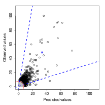
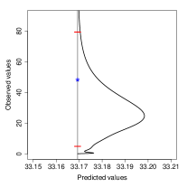
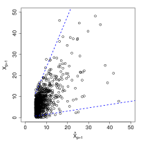
Figure 4: (Left) The estimated joint 95% joint prediction region based on the approximated angular measure $\hat{H}_{(\hat{X}_{p+1},X_{p+1})^{\top}}$. The star indicates a particular observation which has a predicted value of 33.17 and an observed value of 48.15. (Center) The approximate conditional density $f_{X_{p+1}|\hat{X}_{p+1}}(X_{p+1}|\hat{x}_{p+1}=33.17)$. The horizontal segments indicate the $95\%$ conditional prediction interval, and the star denotes the actual value of 48.15. The units of the horizontal axis are the predicted values and the units of the conditional density are omitted. (Right) the scatter plot of $\hat{X}_{p+1}$ and $X_{p+1}$ with $95\%$ conditional prediction intervals given each large value of $\hat{X}_{p+1}.$

6 Applications

6.1 Nitrogen dioxide air pollution.

NO₂ is one of six air pollutants for which the US Environmental Protection Agency (EPA) has national air quality standards. We analyze daily EPA NO₂ data from five locations in the Washington DC metropolitan area (see Figure 1). The first four stations (McMillan 11-001-0043, River Terrace 11-001-0041, Takoma 11-001-0025, Arlington 51-013-0020) have long data records spanning 1995-2020. Alexandria does not have observations after 2016. We will perform prediction at Alexandria given data at the other four locations. Observations in Alexandria actually come from two different stations: 51-510-0009 which has measurements from January1995 to August 2012 and 51-510-00210 from August 2012 to April 2016. Exploratory analysis did not indicate any detectable change point in the Alexandria data either with respect to the marginal distribution or with dependence with other stations, so we treat this data as coming from a single station. There are 5163 days between 1995 and 2016 where all five locations have measurements. Because NO₂ levels have decreased over the study period, we detrend at each location using a moving average mean and standard deviation with window of 901 days to center and scale.

Our inner product space assumes each $X_{i}\in RV_{+}^{1}(\alpha=2)$, and the detrended NO₂ data must be transformed to meet this assumption. In fact, it is unclear whether the NO₂ data are even heavy tailed. Nevertheless, we believe the regular variation framework is useful for describing the tail dependence for this data after marginal transformation. Characterizing dependence after marginal transformation is justified by Sklar’s theorem (Sklar (1959), see also Resnick (1987, Proposition 5.15)), and such transformations are regularly used in multivariate extremes studies. After viewing standard diagnostic plots, we fit a generalized Pareto distribution above each location’s 0.95 quantile and obtain the marginal estimated cdf’s $\hat{F}_{i}$ which are the empirical cdf below the 0.95 quantile and the fitted generalized Pareto above. Letting $X_{i}^{(orig)}$ denote the random variable for detrended NO₂ at location $i$, we define $X_{i}=1/\sqrt{(1-\hat{F_{i}}(X_{i}^{(orig)}))}-\delta$ obtaining a ‘shifted’ Pareto distribution for $i=1,\ldots,5$. Each $X_{i}\in RV_{+}(\alpha=2)$ and the shift $\delta=0.9352$ is such that $\operatorname{E}[t^{-1}(X_{i})]$ = 0. This shift makes the preimages of the transformed data centered which we found reduced bias in the estimation of the TPDM. We assume $\bm{X}=(X_{1},\ldots,X_{5})^{\top}\in RV_{+}^{5}(\alpha=2)$. Further, we let $\bm{X}_{t}$ denote the random vector of observations on day $t$, which we assume to be iid copies of $\bm{X}$. This is a simplifying assumption as there is temporal dependence in the NO₂ data, but it seems less informative that the spatial dependence exhibited by each day’s observations.

We first predict during the period prior to 2015 in order that we can use the observed data at Alexandria to assess performance. Indices are randomly drawn to divide the data set into training and test sets consisting of 3442 and 1721 observations respectively, and both sets cover the entire observational period. Using the training set, the five-dimensional TPDM $\hat{\Sigma}_{\bm{X}}$ is estimated as follows. Let $\bm{x}_{t}$ denote the observed measurements on day $t$. For each $i\neq j$ in $1,\ldots,5$, let $r_{t,ij}=\|(x_{t,i},x_{t,j})\|_{2}$ and $(w_{t,i},w_{t,j})=(x_{t,i},x_{t,j})/r_{t,ij}$. We let $\hat{\sigma}_{ij}=2n_{exc}^{-1}\sum_{t=1}^{n}{w_{t,i}w_{t,j}\mathbb{I}(r_{t,ij}>r^{*}_{ij})}$, where $n_{exc}=\sum_{t=1}^{n}\mathbb{I}(r_{t,ij}>r^{*}_{ij})$. We choose $r^{*}_{ij}$ to correspond to the 0.95 quantile. The constant 2 arises from knowledge that the tail ratio of each $X_{i}$ is one due to the marginal transformation. This pairwise estimation of the TPDM differs from the method in Cooley & Thibaud (2019) who used the entire vector norm as the radial component. Mhatre & Cooley (2020) show that the TPDM is equivalent whether it is defined in terms of the angular measure of the entire vector or the angular measure corresponding to the two-dimensional marginals.

From $\hat{\Sigma}_{\bm{X}}$, we obtain $\hat{X}_{t,5}=\hat{\bm{b}}^{\top}\circ\bm{X}_{t,4}$, where $\hat{\bm{b}}=(-0.047,0.177,0.192,0.482)^{\top}$. We note that the largest weighted component is Arlington, which is closest to Alexandria. Interestingly, McMillan has a slightly negative weight. We calculate $\hat{X}_{t,5}$ for all $t$, but only consider those for which $\hat{X}_{t,5}$ exceeds the 0.95 quantile. The left panel of Figure 5 shows the scatterplot of the values $x_{t,5}$ versus $\hat{x}_{t,5}$. By taking the inverse of the marginal transformation, multiplying by the moving average standard deviation and adding the moving average mean, the predicted value can be put on the scale of the original data. The center panel of Figure 5 shows the scatterplot on the original scale.

We use the method described in Section 5.2 to approximate $H_{(\hat{X}_{p+1},X_{p+1})}$ and use the method described in Section 5.3 to create 95% prediction intervals for each large predicted value $\hat{x}_{t,5}$. We chose the matrix $B$ arising from the completely positive decomposition to be $2\times 9$. Prediction intervals on the Pareto scale are shown in the left panel of Figure 5 and the coverage rate of these intervals is 0.965. The intervals can similarly be back-transformed to be on the original scale as shown in the center panel of Figure 5. The lack of monotonicity in these intervals with respect to the predicted value is due to the trend in the data over the observation period.

For comparison to standard linear prediction, we find the BLUP based on the estimated covariance matrix from the entire data set, and create Gaussian-based 95% confidence intervals from the estimated MSPE. When done on the original data, we obtain a coverage rate of 0.88, and when done on square-root transformed data to account for the skewness, we obtain a coverage rate of 0.78.

We also compare our prediction method to the extremes-based method of Cooley et al. (2012), which approximated the conditional distribution of the large values of a regularly varying variate via a parametric model for the angular measure. The method of Cooley et al. (2012) can be done due to this application’s relatively low dimension. As done in Cooley et al. (2012), the pairwise beta model (Cooley et al., 2010) is fit by maximum likelihood to the preprocessed training data set. The 95% prediction intervals are based on the approximated conditional density of $X_{5}$ given $x_{1},\ldots,x_{4}$, and the achieved coverage rate for the test set is 0.965. Because the fitted angular measure model would seemingly contain more information than the estimated TPDM, we were surprised that the widths of the prediction intervals were very similar for the two methods. The average ratio of Cooley et al. (2012) average interval width to our TPDM-based approach was 1.04.

We then apply our prediction method to five dates in 2019 and 2020 (including January 23, 2020 in Figure 1) when observed values at the four recording stations were large and no observation was taken at Alexandria. Here, we use the entire period from 1995-2016 to estimate the TPDM, and we obtain a slightly different estimate $\hat{\bm{b}}=(0.026,0.153,0.118,0.461)^{\top}$. The right panel of Figure 5 shows the point estimate and 95% prediction intervals from our transformed-linear approach (after back transformation to original scale). The trend at Arlington was used for the unobserved trend at Alexandria. For comparison, covariance matrix-based BLUP’s and MSPE-based 95% prediction intervals for these dates are shown with a dashed line.

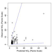
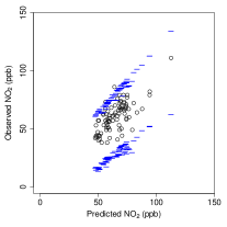
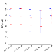
Figure 5: (Left) Scatterplot of $\hat{X}_{5}$ and $X_{5}$ with the 95% prediction intervals on the Pareto scale. (Center) Scatterplot and 95% prediction intervals after transformation to the original scale of the NO₂ data. (Right) Comparison of the point predictions and 95% prediction intervals using the transformed linear approach (solid line) and a Gaussian-based approach (dashed line) for five recent dates when Alexandria is not observed.

6.2 Industry portfolios.

We apply the transformed-linear prediction method to a higher dimensional financial data set. The data set obtained from the Kenneth French Data Library contains the value-averaged daily returns of 30 industry portfolios. We analyze data for 1950-2020, consisting of $n=17911$ observations. Since our interest is in extreme losses, we negate the returns, and set negative returns to zero so that data is in the positive orthant. Although these data appear to be heavy-tailed, it still requires marginal transformation so that $\alpha=2$ can be assumed. Let $\bm{X}^{(orig)}$ denote the random vector of the value-averaged daily returns. For simplicity we use the empirical CDF to perform the marginal transformation $X_{i}=1/\sqrt{(1-\hat{F_{i}}(X_{i}^{(orig)}))}-\delta$, which is applied to each industry’s data so that $X_{i}$ follows the same shifted Pareto distribution as before. We again assume $\bm{X}_{t}$, the random vector denoting the observations on day $t$, are iid copies of $\bm{X}$. A training set consisting of two-thirds of the data ($n_{train}=11940)$ is randomly selected and used to estimate the TPDM and obtain the vector $\hat{\bm{b}}.$ The test set consists of the remaining one-third of the data ($n_{test}=5970)$ to assess coverage rates.

Following similar steps in the previous application, the $30\times 30$ TPDM $\Sigma_{\bm{X}}$ is estimated first in the training set. We focus on performing the linear prediction for extreme losses of coal, beer, and paper. The three largest coefficients in $\hat{\bm{b}}_{coal}$ are $(0.42,0.36,0.20)$ and correspond to fabricated products and machinery, steel, and oil respectively. The three largest coefficients $\hat{\bm{b}}_{beer}$ are $(0.52,0.24,0.12)$ and correspond to food products, retail, and consumer goods (household). The three largest coefficients for $\hat{\bm{b}}_{paper}$ are $(0.21,0.11,0.08)$ and correspond to chemicals, consumer goods (household), and construction materials. The assessed coverage rates of our transformed linear $95\%$ prediction intervals for coal, beer, and paper are $97.9\%$, $96.3\%$, and $98\%$, respectively.

For the purpose of comparison, we also assessed coverage rates of the MSPE-based $95\%$ prediction intervals. Because the data are strongly non-Gaussian, we use the empirical CDF to transform the marginals to be standard normal before estimating the covariance matrix. The coverage rates of MSPE-based 95% prediction intervals are $79.3\%$, $66.6\%$, and $51.2\%$ for coal, beer, and paper respectively.

7 Summary and Discussion

We have proposed a method for performing linear prediction when observations are large. To do so, we constructed an inner product space of nonnegative random variables arising from transformed linear combinations of independent regularly varying random variables. The elements of the TPDM correspond to these inner products if one is willing to assume that these random variables in $\mathcal{V}^{q}_{+}$. The projection theorem yields the optimal transformed linear predictor. Our method for obtaining prediction intervals shows very good performance both in a simulation study and in two applications. The method is simple and is based only on the TPDM which is estimable in high dimensions.

We restrict to nonnegative regularly varying random variables to focus on the upper tail. Relaxing this restriction could allow one to use standard linear operations. Even when the data can be negative, we believe there is value in focusing in one direction. In the financial application, tail dependence for extreme losses is different than for gains, and this information is lost when dependence is summarized with a single number as in the TPDM.

The random vectors $\bm{X}=A\circ\bm{Z}$ comprised of elements of our vector space have a simple angular measure consisting of $q$ point masses where $q$ is the number of columns of $A$. Previous models with angular measures consisting of discrete point masses have been criticized as being overly simple. A difference here is that we do not have to specify $q$ to use this framework to perform prediction, or more generally, we do not have to really believe that our data arise from such a simple model. Rather, if we are comfortable with the information contained in the TPDM, then we can use its information to easily obtain a point prediction and sensible prediction intervals that reflect the information contained.

In many applications, dependence cannot be measured between the observed values and the value to be predicted. In kriging for example, a spatial process model is first fit so that covariance between any two locations is quantified. One can imagine modeling the extremal pairwise dependence as a function of distance before applying the methods here to perform prediction for extreme levels.

References

- (1)
- Cooley et al. (2010) Cooley, D., Davis, R. A. & Naveau, P. (2010), ‘The pairwise beta distribution: A flexible parametric multivariate model for extremes’, Journal of Multivariate Analysis 101(9), 2103–2117.
- Cooley et al. (2012) Cooley, D., Davis, R. A. & Naveau, P. (2012), ‘Approximating the conditional density given large observed values via a multivariate extremes framework, with application to environmental data’, The Annals of Applied Statistics 6(4), 1406–1429.
- Cooley & Thibaud (2019) Cooley, D. & Thibaud, E. (2019), ‘Decompositions of dependence for high-dimensional extremes’, Biometrika 106(3), 587–604.
- De Haan & Ferreira (2007) De Haan, L. & Ferreira, A. (2007), Extreme value theory: an introduction, Springer Science & Business Media.
- Groetzner & Dür (2020) Groetzner, P. & Dür, M. (2020), ‘A factorization method for completely positive matrices’, Linear Algebra and its Applications 591, 1–24.
- Jessen & Mikosch (2006) Jessen, H. A. & Mikosch, T. (2006), ‘Regularly varying functions’, Publications de L’institut Mathematique 80(94), 171–192.
-
Kiriliouk & Zhou (2022)
Kiriliouk, A. & Zhou, C. (2022),
‘Estimating probabilities of multivariate failure sets based on pairwise tail
dependence coefficients’.
https://arxiv.org/abs/2210.12618 - Larsson & Resnick (2012) Larsson, M. & Resnick, S. I. (2012), ‘Extremal dependence measure and extremogram: the regularly varying case’, Extremes 15(2), 231–256.
- Lee (2022) Lee, J. (2022), Linear prediction and partial tail correlation for extremes, PhD thesis, Colorado State University.
- Marron & Ruppert (1994) Marron, J. S. & Ruppert, D. (1994), ‘Transformations to reduce boundary bias in kernel density estimation’, Journal of the Royal Statistical Society: Series B (Methodological) 56(4), 653–671.
-
Mhatre & Cooley (2020)
Mhatre, N. & Cooley, D. (2020),
‘Transformed-linear models for time series extremes’.
https://arxiv.org/abs/2012.06705 - Resnick (1987) Resnick, S. I. (1987), Extreme values, regular variation and point processes, Springer.
- Resnick (2007) Resnick, S. I. (2007), Heavy-tail phenomena: probabilistic and statistical modeling, Springer Science & Business Media.
- Sklar (1959) Sklar, M. (1959), ‘Fonctions de repartition an dimensions et leurs marges’, Publ. inst. statist. univ. Paris 8, 229–231.
- Song & Gupta (1997) Song, D. & Gupta, A. (1997), ‘-norm uniform distribution’, Proceedings of the American Mathematical Society 125(2), 595–601.