Addressing Multiple Salient Object Detection via Dual-Space Long-Range Dependencies

Addressing Multiple Salient Object Detection via
Dual-Space Long-Range Dependencies

Abstract

Salient object detection plays an important role in many downstream tasks. However, complex real-world scenes with varying scales and numbers of salient objects still pose a challenge. In this paper, we directly address the problem of detecting multiple salient objects across complex scenes. We propose a network architecture incorporating non-local feature information in both the spatial and channel spaces, capturing the long-range dependencies between separate objects. Traditional bottom-up and non-local features are combined with edge features within a feature fusion gate that progressively refines the salient object prediction in the decoder. We show that our approach accurately locates multiple salient regions even in complex scenarios. To demonstrate the efficacy of our approach to the multiple salient objects problem, we curate a new dataset containing only multiple salient objects. Our experiments demonstrate the proposed method presents state-of-the-art results on five widely used datasets without any pre-processing and post-processing. We obtain a further performance improvement against competing techniques on our multi-objects dataset. The dataset and source code are available at: https://github.com/EricDengbowen/DSLRDNet.

Introduction

Salient object detection (SOD) aims to highlight the most visually striking or important objects of a scene. SOD plays a significant role in computer vision pipelines, and has been widely applied to many object-level applications in various areas such as object recognition (Rutishauser et al. 2004), object detection (Ren et al. 2013; Zhang et al. 2017), image retrieval (He et al. 2012), image captioning (Das et al. 2017; Fang et al. 2015), weekly supervised semantic segmentation (Wang et al. 2018b; Wei et al. 2016) and image cropping (Wang, Shen, and Ling 2018).

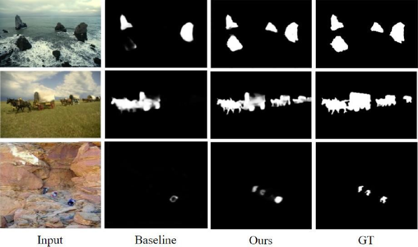
Figure 1: Visual examples of our proposed method. After introducing dual-space long-range dependencies, our model can handle complicated scenes with multiple salient objects.

Although remarkable progress has been made, there still remain many open challenges. Existing SOD datasets contain many images with a single object, often centred in the middle of the image. Human observers may be drawn naturally to centred objects, but in complex scenes they can identify numerous salient objects distributed throughout a scene. Many existing techniques in saliency are based upon traditional U-shape networks, containing only convolutional operations that process local neighborhoods. This fails to exploit the long-range pixel-wise or channel-wise relationships among features in an image, and ultimately leaves techniques less able to address the problem of multiple salient objects (Fig 1). Long-range dependencies have been shown to play an important role in different classification tasks (Wang et al. 2018a), and this is also true of pixel-level segmentation works such as salient object detection. The size of the receptive field is significant in locating and segmenting salient objects across the image. Large kernels aid segmentation tasks but the experimental receptive fields are usually smaller than the ones in theory (Liu et al. 2019; Zhao et al. 2017; Peng et al. 2017). This will likely limit the performance of SOD networks in which objects are spatially separated.

Recent state-of-the-art SOD approaches solve the problem of salient object detection in the general case, often by combining and refining multi-level features into feature representations (Hou et al. 2017; Zhang et al. 2018a; Wu, Su, and Huang 2019a, b; Zhao et al. 2019; Liu et al. 2019), introducing additional losses into frameworks to provide structural information (Feng, Lu, and Ding 2019; Qin et al. 2019) or applying attention mechanisms to filter the redundant information and focus on the valuable features (Zhang et al. 2018b; Liu, Han, and Yang 2018; Chen et al. 2018; Feng, Lu, and Ding 2019; Wu, Su, and Huang 2019a). Only few of the existing SOD methods consider long-range dependencies (Liu, Zhang, and Han 2020; Li, Qi, and Lu 2020; Zhou et al. 2020; Sun, Li, and Guan 2019), and none of these works specifically address the problem of multiple salient objects.

In this paper, we propose a novel architecture for multiple salient object detection that considers long-range dependencies in both spatial space and channel space. Inspired by (Fu et al. 2019; Wang et al. 2018a), we propose a non-local guidance module (NLGM), comprising several dual-space non-local blocks (DSNLBs) to capture pixel-wise and channel-wise relationships. Features at each position are aggregated by a weighted sum of all the features in spatial space, while each channel map is updated by a weighted integration of all interdependent channel maps. Unlike previous work, we stack several DSNLBs in order to capture non-local features in a progressive manner. Bottom-up convolutional features and these non-local features are combined in the network decoder through feature fusion gates, that control the transmission of information into the next stage of the network. These include salient edge supervision to further enhance the quality of the saliency maps. We demonstrate the improved performance of our network on numerous datasets, and specifically multiple salient object detection (MSOD) problems by evaluating on a dataset containing only complex multi-saliency images. Our contributions are:

• We propose a novel MSOD framework that models long-range dependencies in both spatial space and channel space. To the best of our knowledge, this is the first paper that explicitly models long-range dependencies in this dual space for standard SOD and MSOD problems.

• We utilise non-local guidance and edge refinement modules that work complementarily to enrich feature representations at each stage of the top-down pathway. Features from all components are combined within a feature fusion gate, which utilises edge features to promote relevant salient and non-local features. The fusion gate ensures that top-down features are passed discriminatively through the network.

• We curate a new dataset containing only multiple salient objects, drawn from popular datasets in this field. We compare the proposed approach against 14 state-of-the-art methods on five widely used SOD benchmarks and the proposed multi-object dataset. Without any pre-processing and post-processing, our proposed method exceeds all previous state-of-the-art approaches in three evaluation metrics and provides a further performance boost against competing techniques on our proposed dataset.

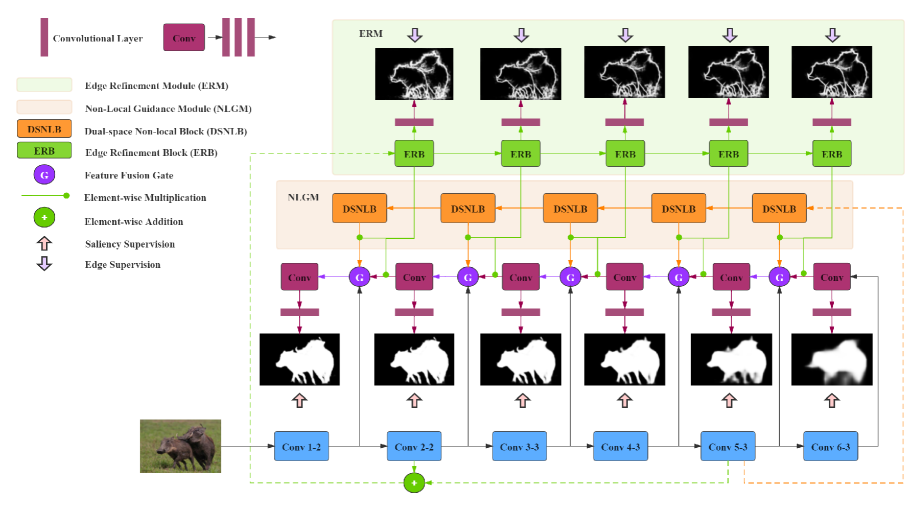
Figure 2: The overall pipeline of our proposed approach, here shown using a VGG backbone. The red, orange and green boxes capture saliency features, non-local features and edge features respectively. Element-wise multiplication operates between each pair of ERB-DSNLB (edge and non-local features) and ERB-Conv (edge and saliency features). Our final prediction map is generated based on the fusion of 6 multi-scale saliency features in top-down pathway.

Related Work

Traditional salient object detection methods mostly rely on low-level features (Zhu et al. 2014; Jiang et al. 2013) or heuristic priors such as colour contrast (Cheng et al. 2014) and background (Wei et al. 2012; Yang et al. 2013). More details are introduced in the survey by Borji et al.(Borji et al. 2019).

Early deep SOD methods utilised multi-scale image patches (Li and Yu 2015; Wang et al. 2015), offering impressive performance, but limited by the lack of spatial information found in small image patches. Since the introduction of fully convolutional networks (FCNs) (Long, Shelhamer, and Darrell 2015), there have been many effective and efficient end-to-end SOD architectures. Among these, U-shape based architectures (Ronneberger, Fischer, and Brox 2015) see much use. Hou (Hou et al. 2019, 2017) applied short connections from deeper to shallower layers, integrating high-level and low-level features. Zhang et al.(Zhang et al. 2018a) used a gated pathway for bi-directional message passing and multi-level feature integration. Zhang et al.(Zhang et al. 2018b) embedded multi-path recurrent connections and spatial attention modules to generate saliency maps. Chen et al.(Chen et al. 2018) designed a reverse attention block to emphasize non-object areas. Qin et al.(Qin et al. 2019) applied another bottom-up/top-down architecture to refine the coarse saliency map generated from the prediction network. This work generates boundary-aware saliency maps through a hybrid loss approach. Feng et al.(Feng, Lu, and Ding 2019) employed global perceptron modules and attentive feedback modules to detect global saliency and build encoder-decoder communication respectively. Zhao et al.(Zhao et al. 2019) explicitly modeled edge features to guide the multi-scale features extracted from a U-shape structure and then fused multiple side-outputs into a final saliency map. Liu et al.(Liu et al. 2019) mainly investigated the role of pooling layer in U-shape structure. They proposed a global guidance module for transmitting localization information to top-down pathway and a feature aggregation module to further refine fused features. Wu et al.(Wu, Su, and Huang 2019b) introduced a cross refinement unit to exchange mutual information between edge features and saliency features. Zhao et al.(Zhao et al. 2020) designed a gated dual branch network incorporating a Fold-ASPP to better localise the salient objects of various scales. Pang et al.(Pang et al. 2020) proposed a transformation-interaction-fusion strategy to obtain efficient multi-scale features and a consistency-enhanced loss to deal with the imbalance issue between foreground and background.

Existing SOD methods seldom consider long-range dependencies: the sharing of information across spatially distant pixels, or between feature maps in channel space. Of those that do, Li et al.(Li, Qi, and Lu 2020) and Sun et al.(Sun, Li, and Guan 2019) applied self-attention mechanisms to capture spatial long-range context. Zhou et al.(Zhou et al. 2020) introduced a multi-type self-attention to capture pixel-level relationships for saliency detection in degraded images. Liu et al.(Liu, Zhang, and Han 2020) designed a self-mutual attention to capture long-range contextual dependencies, this time in RGB-D. Of these works, none have made use of channel-wise dependencies as we do here and there is no ideal solution for multiple salient object detection. This has previously been hard to examine; existing public datasets contain some multi-object instances, but the frequency of these varies substantially. Here we curate a dataset specifically for this purpose, allowing us to focus on this problem.

Proposed Method

The architecture of our proposed method is shown in Fig 2. Our model is based on a U-shape FCN combining a bottom-up pathway (backbone) and a top-down pathway. Similar to most deep SOD models, we use VGG network to illustrate our proposed structure. Following EGNet (Zhao et al. 2019) and DSS (Hou et al. 2017, 2019), the last three fully connected layers are truncated and an additional side path is connected to the last pooling layer of VGG. This provides 6 outputs from bottom-up pathway representing the multi-level features captured from Conv1-2 to Conv6-3, which can be defined as a feature set $S=\left\{S^{1},S^{2},S^{3},S^{4},S^{5},S^{6}\right\}$.

Multi-scale saliency features are processed through the top-down pathway with a series of convolutional blocks, each containing 3 convolutional layers and ReLU activations. We refer to this saliency feature set as $F=\left\{F^{1},F^{2},F^{3},F^{4},F^{5},F^{6}\right\}$, where $F^{6}$ is the saliency feature produced by the sixth convolutional block (rightmost Conv in Fig 2) and so on.

We leverage intermediate supervision (Lee et al. 2015) at each convolutional block to improve training performance. For each saliency feature $F^{i}$, a convolutional layer $D^{i}_{F}$ is applied to produce a single-channel prediction. We use a cross-entropy loss, with the supervision here defined as:

$$\mathcal{L}^{i}_{F}\left(F^{i},W_{DF}^{i}\right)=-\sum_{j\in{Y^{+}}}\log Pred\left(y_{j}=1|F^{i};W_{DF}^{i}\right)\\ -\sum_{j\in{Y^{-}}}\log Pred\left(y_{j}=0|F^{i};W_{DF}^{i}\right),i\in\left[1,6\right],$$ (1)

where $Y^{+}$ and $Y^{-}$ denote the pixels in salient region and non-salient region respectively. $W_{DF}^{i}$ denotes the parameters of convolutional layer $D^{i}_{F}$. $Pred\left(y_{j}=1|F^{i};W_{DF}^{i}\right)$ denotes the salient prediction map.

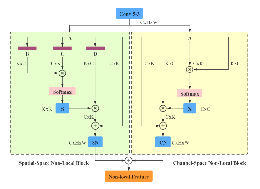
Figure 3: The architecture of a dual-space non-local block (DSNLB). $C$, $H$ and $W$ demonstrate the channel number, height and width of given feature map respectively and $K=H\times W$.

Non-Local Guidance Module

In this module we model long-range dependencies in both spatial and channel space. Inspired by (Fu et al. 2019), we make use of dual-space non-local information within two parallel pathways that capture pixel-wise contextual information and channel-wise relationships. Unlike (Fu et al. 2019), which directly append a single attention module on top of FCN for scene segmentation, our NLGM is composed of 5 stacked dual-space non-local blocks (DSNLBs), one at each stage of the top-down pathway. We choose the feature map $S^{5}$ extracted from Conv5-3 as the input of the NLGM as it contains high-level semantic information, and yet contains more spatial information than $S^{6}$. Fig 3 illustrates the detailed structure of the first DSNLB.

Spatial-Space Non-Local Block:

For a given feature map $\mathbf{A}\in\mathds{R}^{C\times H\times W}$, 3 convolutional layers are used to generate 3 distinct feature maps $\left\{\mathbf{B,C,D}\right\}\in\mathds{R}^{C\times H\times W}$, representing query, key and value respectively. $\mathbf{B,C}$ and $\mathbf{D}$ are reshaped to $\mathds{R}^{C\times K}$, where $K=H\times W$. A unified similarity matrix $\mathbf{S}\in\mathds{R}^{K\times K}$ is calculated as:

$$\mathbf{S}=f(\mathbf{B}^{\mathrm{T}}\times\mathbf{C}).$$ (2)

We apply a $softmax$ normalisation function for $f$ here. The weight matrix $\mathbf{S}$ models the affinity of features between any two spatial positions. The final weighted feature map $SN$ in spatial space can be defined as:

$$SN=(\mathbf{S}^{\mathrm{T}}\times\mathbf{D})^{\mathrm{T}}+\mathbf{A},$$ (3)

where $SN\in\mathds{R}^{C\times H\times W}$ after reshaping. Informally, $SN$ may be thought of as an enriched feature representation with global spatial perception, as each value of $SN$ is a selective weighted sum of all positions across the whole feature map.

Channel-Space Non-Local Block

Given same feature map $\mathbf{A}\in\mathds{R}^{C\times H\times W}$, reshaped to $\mathds{R}^{C\times K}$, the unified similarity matrix $\mathbf{X}\in\mathds{R}^{C\times C}$ in channel space is calculated as:

$$\mathbf{X}=f(\mathbf{A}\times\mathbf{A}^{\mathrm{T}}),$$ (4)

where $f$ indicates $softmax$ function and $\mathbf{X}$ measures the correlation between any two channels. The weighted feature map $CN$ in channel space can be defined as:

$$CN=(\mathbf{X}^{\mathrm{T}}\times\mathbf{A})+\mathbf{A},$$ (5)

where $CN\in\mathds{R}^{C\times H\times W}$ is a feature representation containing long-range dependencies within channel space.

Non-Local Feature Aggregation

We combine the above features $SN$ and $CN$ to generate our non-local feature representations $N$, exploiting long-range contextual information in both spatial and channel space. $N$ is given as:

$$N=D_{N}(SN+CN),$$ (6)

where $D_{N}$ is a $1\times 1$ convolutional layer.

Multi-Hop Communications

Our NLGM is composed of 5 DSNLBs, each generating non-local features $N^{i}$ at each stage of top-down pathway. By stacking several DSNLBs, non-local features are progressively refined through multi-hop communication between features that share affinity both channel-wise and spatially. Relevant saliency-specific semantic information is shared across the image space and feature space. Since non-local features have a global view, the challenge of complex scenes and multiple salient objects are better addressed through this improved receptive field.

Feature Fusion

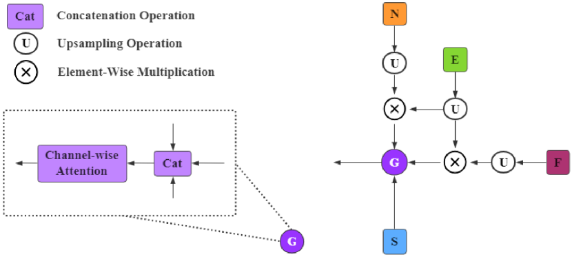
Figure 4: The structure of a feature fusion gate. $N$, $E$, $F$ and $S$ demonstrate non-local feature, edge feature, saliency feature and the corresponding side output of bottom-up pathway respectively.

The majority of the existing SOD models fuse different features without distinction. Redundant and mutually incompatible features from different objectives may harm overall performance once combined. As presented in Fig 4, we leverage channel-wise attention to selectively aggregate different features at each stage of top-down pathway.

Edge Refinement Module

Motivated by the commonly used boundary detection in SOD models (Qin et al. 2019; Zhao et al. 2019), salient edge features are modeled, as part of the feature fusion gate, to support the training of non-local and salient features. Edge features are generated from low-level features $S^{2}$ and high-level features $S^{5}$ through bottom-up process, which are progressively refined within an Edge Refinement Module (ERM). We found that $S^{2}$ and $S^{5}$ outperformed $S^{1}$ and $S^{6}$ in this role. $S^{1}$ is lower level with a reduced receptive field size, while $S^{6}$ is high level, but has limited resolution.

The Edge Refinement Module (ERM) consists of 5 edge refinement blocks (ERBs) aligned with the respective blocks in the NLGM. Each ERB contains a convolutional layer followed by a ReLU function to generate salient edge features $E^{i}$ at each stage. As with the salient features, we apply intermediate supervision in the ERM via a cross-entropy loss. A convolutional layer $D_{E}^{i}$ is used to convert the edge feature to single-channel prediction map. The supervision here can be defined as:

$$\mathcal{L}^{i}_{E}\left(E^{i},W_{DE}^{i}\right)=-\sum_{j\in{V^{+}}}\log Pred\left(y_{j}=1|E^{i};W_{DE}^{i}\right)\\ -\sum_{j\in{V^{-}}}\log Pred\left(y_{j}=0|E^{i};W_{DE}^{i}\right),i\in\left[1,5\right],$$ (7)

where $V^{+}$ and $V^{-}$ denote the set of salient edge pixels and other pixels respectively. $W_{DE}$ indicates the parameters of $D_{E}^{i}$. We weight the two components of the above loss by the number of pixels in each class.

Feature Fusion Gate

Salient edge features are combined with salient and non-local features separately through element-wise multiplication. This operation serves to emphasise activations that are shared between feature maps, promoting complimentarity between the non-local, saliency and edge features. Features that are aligned between modules will train more quickly, with activations of those that are less relevant to other blocks reduced. The resulting salient and non-local features are then combined using channel-wise attention. Firstly, we unify the spatial size and channel count:

$$\hat{N^{i}}=Up(\delta(O(N^{i};\theta));S^{i}),i\in[1,5],$$ (8)

$$\hat{F^{i}}=Up(\delta(O(F^{i};\theta));S^{i+1}),i\in[2,6],$$ (9)

$$\hat{E^{i}}=Up(\delta(O(E^{i};\theta));S^{i}),i\in[1,5],$$ (10)

where $Up(*;S^{i})$ upsamples $*$ to be the same size as $S^{i}$. $O(*;\theta)$ denotes a convolutional layer with parameter $\theta$ and $\delta$ is a ReLU activation function, which converts the channel number of $*$ to the channel number of $S^{i}$. The fused features $F^{i}_{fusion}$, including the incorporation of salient edge features, are calculated as:

$$F^{i}_{fusion}=CA(Cat(S^{i},\hat{N^{i}}\otimes\hat{E^{i}},\hat{F}^{i+1}\otimes\hat{E^{i}})),$$ (11)

where $\otimes$ denotes the element-wise multiplication. $Cat$ is the concatenation operation. $CA$ indicates the channel-wise attention, which can be defined as:

$$CA(*,\theta_{ca})=*\cdot(\sigma(fc_{2}(\delta(fc_{1}(ap(*,\theta_{1}))),\theta_{2}))),$$ (12)

where $\theta_{ca}$ denotes the parameters in channel-wise attention, $ap$ is a global average pooling layer and $fc$ is a fully-connected layer. $\sigma$ and $\delta$ refer to the sigmoid function and ReLU functions respectively. The feature fusion gate here provides a mechanism to select the most useful channels for saliency from each module, fusing features with distinction.

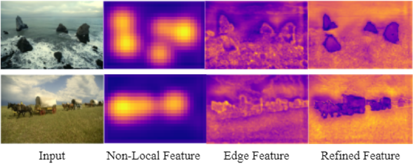
Figure 5: Feature visualization of non-local features, edge features and the refined features after feature fusion. As can be seen, our non-local features highlight objects across the scene. After the feature fusion, multiple salient objects are clearly defined.

Saliency Inference

To make full use of the multi-scale saliency features, we hierarchically generate the final prediction map based on the fusion of six saliency features $F^{i}$ from coarse-to-fine manner. This multi-scale fusion strategy also serves to reduce the risk of missing salient objects across multi-saliency visual scenes. Complementary features $F^{2},F^{3},F^{4},F^{5},F^{6}$ are upsampled and convolved to have equal spatial and feature size to $F^{1}$, they are then combined using element-wise addition to produce a final feature $F_{fin}$. A convolutional layer $D_{P}$ is used to convert the feature map $F_{fin}$ to a single-channel prediction map, trained using cross entropy:

$$\mathcal{L}_{fin}\left(F_{fin},W_{P}\right)=-\sum_{j\in{Y^{+}}}\log Pred\left(y_{j}=1|F_{fin};W_{P}\right)\\ -\sum_{j\in{Y^{-}}}\log Pred\left(y_{j}=0|F_{fin};W_{P}\right),$$ (13)

where $Y^{+}$ and $Y^{-}$ denote the set of salient pixels and non-salient pixels respectively. $W_{P}$ refers to the parameters of convolutional layer $D_{P}$. Therefore the total loss $\mathds{L}$ in our proposed method can be denoted as:

$$\mathds{L}=\sum_{i=1}^{6}\mathcal{L}_{F}^{i}(F^{i};W_{DF}^{i})+\sum_{i=1}^{5}\mathcal{L}_{E}^{i}(E^{i};W_{DE}^{i})\\ +\mathcal{L}_{fin}\left(F_{fin},W_{P}\right)$$ (14)

Experiments

Datasets:

To demonstrate the performance of our proposed method, we evaluate our model on five widely used benchmark datasets: DUT-OMRON (Yang et al. 2013), HKU-IS (Li and Yu 2015), DUTS (Wang et al. 2017), ECSSD (Yan et al. 2013) and SOD (Movahedi and Elder 2010). Scenes including multiple salient objects do exist in each dataset, but the frequency varies from a minimum of 9.8% for ECSSD to 50.3% for HKU-IS, with an average across the datasets of 28%. Of these multi-object images, the majority contain only two objects. Metrics calculated across these datasets will respond to model performance specific to multiple objects, but evaluation is challenging. Here, we curate a new dataset, MSOD, containing the most challenging multi-object scenes across the five datasets. In order to evaluate our, and other methods on complex multi-object images, scenes were only included if they contained three or more salient objects. The total MSOD dataset comprises 300 test images with 1342 total objects. The number of objects in each image varies from 3 to 19 and the distribution is shown in Fig 6. The dataset comprises a variety of object classes, and a varied number of these objects across the image. We observed that the objects did not exhibit any particular predictable spatial locations.

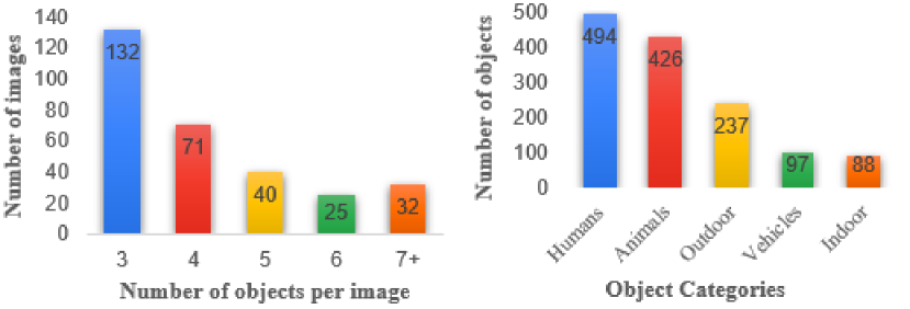
Figure 6: The distribution of the proposed MSOD dataset.

Evaluation Metrics:

Three widely used metrics are applied for performance evaluation: F-measure, mean absolute error (MAE) and the structure-based metric S-measure (Fan et al. 2017). F-measure is a weighted harmonic mean of precision and recall, defined as:

$$F_{\beta}=\frac{(1+\beta^{2})\times Precision\times Recall}{\beta^{2}\times Precision+Recall}$$ (15)

where $\beta^{2}$ is commonly set to 0.3 in previous works to emphasize precision. Following most state-of-the-art SOD approaches, we report the maximum $F_{\beta}$ from all pairs of precision and recall on different thresholds. We also use MAE to compare the prediction map $P$ and ground truth $Y$, of size $W\times H$, defined as:

$$MAE=\frac{1}{W\times H}\sum_{i=1}^{W}\sum_{j=1}^{H}{|P(i,j)-Y(i,j)|}$$ (16)

Finally, we use S-measure to consider both the region-aware $S_{r}$ and object-aware $S_{o}$ structural similarity, defined as:

$$S=\alpha\times S_{0}+\left(1-\alpha\right)\times S_{r}$$ (17)

where $\alpha$ is set to 0.5 by default. More details about S-measure can be found in (Fan et al. 2017).

	ECSSD			DUTS-TE			HKU-IS			DUT-O			SOD			MSOD
	1000 images			5019 images			1447 images			5168 images			300 images			300 images
Model	MaxF $\uparrow$	MAE $\downarrow$	S $\uparrow$	MaxF $\uparrow$	MAE $\downarrow$	S $\uparrow$	MaxF $\uparrow$	MAE $\downarrow$	S $\uparrow$	MaxF $\uparrow$	MAE $\downarrow$	S $\uparrow$	MaxF $\uparrow$	MAE $\downarrow$	S $\uparrow$	MaxF $\uparrow$	MAE $\downarrow$	S $\uparrow$
VGG-Backbone
DSS (CVPR2017)	.9207	.0517	.8821	.8251	.0565	.8237	.9161	.0401	.8783	.7812	.0628	.7899	.8410	.1201	.7478	.8240	.0550	.7806
BDMP (CVPR2018)	.9284	.0446	.9109	.8514	.0490	.8616	.9205	.0389	.9065	.7739	.0636	.8091	.8517	.1057	.7833	.8401	.0538	.8379
PAGR (CVPR2018)	.9259	.0608	.8883	.8540	.0555	.8383	.9187	.0475	.8891	.7706	.0709	.7751	.8358	.1447	.7137	.8204	.0627	.7852
RAS (ECCV2018)	.9211	.0564	.8928	.8311	.0594	.8385	.9128	.0454	.8874	.7864	.0617	.8141	.8473	.1225	.7608	.8370	.0597	.8167
BASNet (CVPR2019)	.9425	.0370	.9162	.8594	.0476	.8656	.9297	.0329	.9077	.8052	.0565	.8361	.8487	.1119	.7660	.8396	.0541	.8306
AFNet (CVPR2019)	.9350	.0418	.9134	.8628	.0458	.8666	.9252	.0355	.9058	.7970	.0573	.8258	.8499	.1087	.7700	.8276	.0547	.8191
Ours	.9485	.0344	.9261	.8894	.0381	.8878	.9350	.0300	.9167	.8194	.0541	.8421	.8761	.0996	.7922	.8531	.0478	.8410
ResNet-Backbone
PiCANet (CVPR2018)	.9349	.0464	.9170	.8597	.0506	.8686	.9193	.0437	.9045	.8027	.0653	.8318	.8528	.1024	.7871	.8190	.0641	.8223
PoolNet (CVPR2019)	.9489	.0350	.9263	.8891	.0368	.8865	.9358	.0300	.9187	.8048	.0539	.8309	.8706	.1034	.7854	.8546	.0459	.8429
EGNet (ICCV2019)	.9474	.0374	.9247	.8885	.0392	.8868	.9352	.0309	.9179	.8152	.0531	.8408	.8778	.0969	.8000	.8516	.0470	.8402
CPD (CVPR2019)	.9393	.0371	.9181	.8653	.0434	.8689	.9252	.0339	.9064	.7964	.0560	.8247	.8568	.1095	.7646	.8241	.0539	.8109
SCRN (ICCV2019)	.9496	.0375	.9272	.8875	.0398	.8847	.9351	.0332	.9169	.8112	.0560	.8364	.8655	.1046	.7851	.8384	.0527	.8244
GateNet (ECCV2020)	.9454	.0401	.9198	.8873	.0401	.8847	.9334	.0331	.9153	.8178	.0549	.8380	.8731	.0981	.7948	.8623	.0483	.8507
MINet (CVPR2020)	.9475	.0335	.9249	.8836	.0372	.8837	.9353	.0283	.9197	.8097	.0555	.8325	.8730	.0905	.7973	.8472	.0474	.8400
SCWSSOD* (AAAI2021)	.9145	.0489	.8818	.8440	.0487	.8405	.9111	.0375	.8824	.7823	.0602	.8117	.8367	.1077	.7503	.8329	.0534	.8060
Ours	.9519	.0325	.9297	.8967	.0358	.8946	.9389	.0293	.9218	.8234	.0530	.8470	.8786	.0934	.8024	.8720	.0442	.8614

Table 1: Quantitative comparison with other state-of-the-art methods on 5 widely used datasets and the proposed MSOD dataset. $\uparrow$ and $\downarrow$ indicate higher or lower is better respectively and * denotes weakly-supervised methods. The best three results among both backbones are marked as red, blue and cyan. Our method achieves top results under 3 evaluation metrics across all datasets without any pre-processing and post-processing.

Models			DUTS-TE			DUT-OMRON
NLGM	FFG	ERM	MaxF $\uparrow$	MAE $\downarrow$	S $\uparrow$	MaxF $\uparrow$	MAE $\downarrow$	S $\uparrow$
			.8761	.0425	.8750	.7958	.0575	.8276
✓			.8836	.0410	.8809	.8103	.0562	.8357
✓		✓	.8847	.0410	.8839	.8138	.0563	.8366
✓	✓		.8858	.0396	.8857	.8153	.0560	.8379
✓	✓	✓	.8894	.0381	.8878	.8194	.0541	.8421

Table 2: Ablation analysis of different components in our proposed architecture.

NLGM Configurations	DUTS-TE			DUT-OMRON
	MaxF $\uparrow$	MAE $\downarrow$	S $\uparrow$	MaxF $\uparrow$	MAE $\downarrow$	S $\uparrow$
SSNLB	.8813	.0411	.8789	.8081	.0563	.8336
CSNLB	.8816	.0415	.8790	.8079	.0566	.8348
SSNLB+CSNLB	.8836	.0410	.8809	.8103	.0562	.8357

Table 3: Performance comparison of different NLGM configurations. SSNLB and CSNLB refer to spatial-space non-local block and channel-space non-local block respectively. All three configurations are without FFG and ERM.

Implementation Details:

The proposed approach is implemented in PyTorch and trained on the DUTS-TR (Wang et al. 2017) dataset, where the salient edge ground truth is calculated by sober operator. To compare our method against other state-of-the-art methods, we train our model using both VGG (Simonyan and Zisserman 2014) and Resnet-50 (He et al. 2016) backbones. The parameters of backbones are initialized using pretrained models on ImageNet (Krizhevsky, Sutskever, and Hinton 2012), while the weights of newly added layers are initialized randomly. We use the Adam (Kingma and Ba 2014) optimizer with an initial learning rate of 2e-5, which is divided by 10 after 30 epochs. Our model is trained for 40 epochs in total, which tipically takes 3 days in a single 2080Ti with a forward pass taking 0.02s.

Comparisons with the State-of-the-Art

We compare our proposed method against 14 recent state-of-the-art methods: DSS (Hou et al. 2017), BDMP (Zhang et al. 2018a), PAGR (Zhang et al. 2018b), PiCANet (Liu, Han, and Yang 2018), RAS (Chen et al. 2018), BASNet (Qin et al. 2019), AFNet (Feng, Lu, and Ding 2019), PoolNet (Liu et al. 2019), EGNet (Zhao et al. 2019), CPD (Wu, Su, and Huang 2019a), SCRN (Wu, Su, and Huang 2019b), GateNet (Zhao et al. 2020), MINet (Pang et al. 2020) and SCWSSOD (Yu et al. 2021). For fair comparison, all the saliency maps of competing methods were produced by either pre-trained models, or pre-generated by the authors.

Quantitative Comparison:

Table 1 shows that our proposed method achieves the best result under 3 evaluation metrics across the datasets. Against the current top approaches: MINet (Pang et al. 2020), PoolNet (Liu et al. 2019), EGNet (Zhao et al. 2019) and SCRN (Wu, Su, and Huang 2019b), the average improvement of our proposed method on 5 widely used datasets is 0.92%, 2.27%, 2.43% and 4.09% respectively. A further performance improvement can be observed in MSOD dataset, with the average improvement over these approaches increasing to 4.08%, 2.64%, 3.63% and 8.21% respectively. This demonstrates the strong multiple salient object detection ability of our proposed method, which obtains state-of-the-art performance on this challenging dataset.

Precision-Recall Curves:

We plot precision-recall curves over 3 popular SOD datasets and the proposed MSOD dataset in Fig 7. Our proposed method outperforms all other approaches at most thresholds, especially in the two largest datasets DUT-OMRON and DUTS-TE.

Visual Comparison:

Qualitative results of our method can be seen in Fig 8, where our method provides excellent performance in multi-saliency images. Our use of non-local features and top-down feature fusion can make full use of the long-range dependencies between salient objects, with information shared between separate regions of the image.

Ablation Studies

In this section we investigate the contribution of different components in our proposed approach. All experiments are based on VGG backbone and two largest datasets: DUTS-TE and DUT-OMRON.

Effectiveness of NLGM:

Compared to a baseline structure (1 row in Table 2), non-local guidance (2 row) provides performance gains across all evaluation metrics on both datasets. This demonstrates the effectiveness of capturing long-range dependencies in NLGM.

Effectiveness of FFG:

Incorporating feature fusion (the 4 and 5 row in Table 2) can also improve the performance beyond the ones without FFG across all metrics on both datasets, indicating the importance of filtering the redundant information from each part of the architecture.

Effectiveness of NLGM & ERM:

Compared to 2 row, the 3 row in Table 2 has a higher performance, which proves the effectiveness of introducing both NLGM and ERM. Features that are mutually beneficial to both non-local and edge saliency are emphasised. These modules appear to complement each other, with non-local, edge and saliency all contributing to the accurate recovery of salient regions.

Effectiveness of FFG & ERM:

By introducing edge features as part of the FFG, performance gains can be observed (5 row and 4 row in Table 2), which demonstrates that the edge refinement module effectively promotes relevant salient features prior to their combination within the FFG.

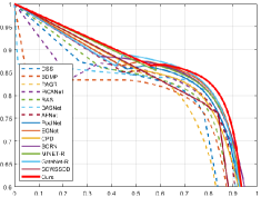
(a) DUT-OMRON

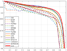
(b) DUTS-TE

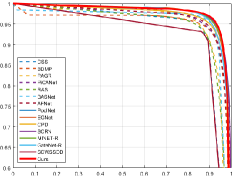
(c) ECSSD

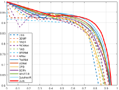
(d) MSOD

Figure 7: Precision (vertical axis) recall (horizontal axis) curves on three popular salient object detection datasets and the proposed MSOD dataset. The red solid line demonstrates our proposed method.

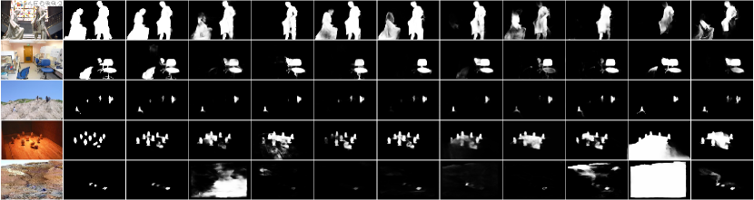
Image

GT

Ours

GateNet

MINet

PoolNet

EGNet

SCRN

PAGR

RAS

BASNet

AFNet

Figure 8: Qualitative comparisons with state-of-the-art approaches over some of the challenging images.

Architectures of NLGM:

We perform experiments to explore the effect of different structures of NLGM. We evaluate four different architectures to incorporate non-local information into our U-shape network. The architectures and the corresponding performance are shown in Fig 9 and Table 4. Our baseline model (a) utilises a single DSNLB drawing features from $S^{6}$, with the same output distributed to all top-down stages. Model (b) incorporates a stack of 5 DSNLBs in this same construction, evaluating the effect of chains of non-local blocks over single instances. We find that a stack of DSNLBs improve performance on all metrics, indicating the effectiveness of long-range multi-hop communications that build richer relevant salient features across both spatial and channel space. Model (c) draws features again from $S^{6}$ but distributes the DSNLBs throughout the top-down pathway as per our main architecture in fig 2. Performance is again improved a little, likely because this one-to-one guidance method can generate adaptive non-local features appropriate to each scale of saliency features $F$. Finally, model (d) draws features from $S^{5}$ as our final architecture does. The improvement suggests that the increased spatial size of these features is better exploited by the DSNLBs over the relatively small spatial size of that in $S^{6}$.

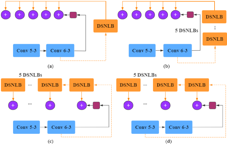
Figure 9: Different architectures of NLGM. All structures here are without FFG and ERGM. Element-wise addition operation is used at each stage to fuse different features.

NLGM Architectures	DUTS-TE			DUT-OMRON
	MaxF $\uparrow$	MAE $\downarrow$	S $\uparrow$	MaxF $\uparrow$	MAE $\downarrow$	S $\uparrow$
(a)	.8796	.0419	.8787	.8052	.0567	.8313
(b)	.8815	.0415	.8801	.8075	.0565	.8330
(c)	.8816	.0417	.8805	.8083	.0565	.8345
(d)	.8836	.0410	.8809	.8103	.0562	.8357

Table 4: Performance comparison of different NLGM architectures. All structures here are without FFG and ERM.

Configurations of NLGM:

As shown in Table 3, we conduct experiments to investigate the performance of different configurations of NLGM. Compared to the baseline (the 1 row in Table 2), the models incorporating SSNLB (the 1 row in Table 3) or CSNLB (the 2 row in Table 3) both improve performance on two datasets. The best performance is obtained when using both SSNLB and CSNLB together (the 3 row in Table 3), showing that these two modules are highly complimentary, and that both spatial and channel-wise non-local features contribute to image saliency.

Conclusion

In this paper we seek to address the problem of segmenting multiple salient objects in complex scenes. We present a new architecture for salient object detection, utilising both spatial and channel-wise long-range dependencies. A non-local guidance module captures long-range dependencies between salient objects across the image, allowing the network to better resolve multiple separate salient objects. We also design a feature fusion gate that combines salient and non-local features. The gate utilises progressively refined edge features to promote the most relevant features drawn from each module. Our approach shows state-of-the-art performance across 5 widely used salient object datasets. We also curate an additional dataset comprising only multiple objects in challenging scenes, and show that the performance gap between ours and other methods widens. Consideration of complex scenes is required to further drive development in image saliency, our network and the new dataset can be used as a baseline for performance in this domain.

References

- Borji et al. (2019) Borji, A.; Cheng, M.-M.; Hou, Q.; Jiang, H.; and Li, J. 2019. Salient object detection: A survey. Computational visual media, 1–34.
- Chen et al. (2018) Chen, S.; Tan, X.; Wang, B.; and Hu, X. 2018. Reverse attention for salient object detection. In Proceedings of the European Conference on Computer Vision (ECCV), 234–250.
- Cheng et al. (2014) Cheng, M.-M.; Mitra, N. J.; Huang, X.; Torr, P. H.; and Hu, S.-M. 2014. Global contrast based salient region detection. IEEE transactions on pattern analysis and machine intelligence, 37(3): 569–582.
- Das et al. (2017) Das, A.; Agrawal, H.; Zitnick, L.; Parikh, D.; and Batra, D. 2017. Human attention in visual question answering: Do humans and deep networks look at the same regions? Computer Vision and Image Understanding, 163: 90–100.
- Fan et al. (2017) Fan, D.-P.; Cheng, M.-M.; Liu, Y.; Li, T.; and Borji, A. 2017. Structure-measure: A new way to evaluate foreground maps. In Proceedings of the IEEE international conference on computer vision, 4548–4557.
- Fang et al. (2015) Fang, H.; Gupta, S.; Iandola, F.; Srivastava, R. K.; Deng, L.; Dollár, P.; Gao, J.; He, X.; Mitchell, M.; Platt, J. C.; et al. 2015. From captions to visual concepts and back. In Proceedings of the IEEE conference on computer vision and pattern recognition, 1473–1482.
- Feng, Lu, and Ding (2019) Feng, M.; Lu, H.; and Ding, E. 2019. Attentive feedback network for boundary-aware salient object detection. In Proceedings of the IEEE Conference on Computer Vision and Pattern Recognition, 1623–1632.
- Fu et al. (2019) Fu, J.; Liu, J.; Tian, H.; Li, Y.; Bao, Y.; Fang, Z.; and Lu, H. 2019. Dual attention network for scene segmentation. In Proceedings of the IEEE Conference on Computer Vision and Pattern Recognition, 3146–3154.
- He et al. (2012) He, J.; Feng, J.; Liu, X.; Cheng, T.; Lin, T.-H.; Chung, H.; and Chang, S.-F. 2012. Mobile product search with bag of hash bits and boundary reranking. In 2012 IEEE Conference on Computer Vision and Pattern Recognition, 3005–3012. IEEE.
- He et al. (2016) He, K.; Zhang, X.; Ren, S.; and Sun, J. 2016. Deep residual learning for image recognition. In Proceedings of the IEEE conference on computer vision and pattern recognition, 770–778.
- Hou et al. (2019) Hou, Q.; Cheng, M.; Hu, X.; Borji, A.; Tu, Z.; and Torr, P. 2019. Deeply supervised salient object detection with short connections. IEEE Transactions on Pattern Analysis and Machine Intelligence, 41(4).
- Hou et al. (2017) Hou, Q.; Cheng, M.-M.; Hu, X.; Borji, A.; Tu, Z.; and Torr, P. H. 2017. Deeply supervised salient object detection with short connections. In Proceedings of the IEEE Conference on Computer Vision and Pattern Recognition, 3203–3212.
- Jiang et al. (2013) Jiang, H.; Wang, J.; Yuan, Z.; Wu, Y.; Zheng, N.; and Li, S. 2013. Salient object detection: A discriminative regional feature integration approach. In Proceedings of the IEEE conference on computer vision and pattern recognition, 2083–2090.
- Kingma and Ba (2014) Kingma, D. P.; and Ba, J. 2014. Adam: A method for stochastic optimization. arXiv preprint arXiv:1412.6980.
- Krizhevsky, Sutskever, and Hinton (2012) Krizhevsky, A.; Sutskever, I.; and Hinton, G. E. 2012. Imagenet classification with deep convolutional neural networks. In Advances in neural information processing systems, 1097–1105.
- Lee et al. (2015) Lee, C.-Y.; Xie, S.; Gallagher, P.; Zhang, Z.; and Tu, Z. 2015. Deeply-supervised nets. In Artificial intelligence and statistics, 562–570.
- Li, Qi, and Lu (2020) Li, A.; Qi, J.; and Lu, H. 2020. Multi-attention guided feature fusion network for salient object detection. Neurocomputing, 411: 416–427.
- Li and Yu (2015) Li, G.; and Yu, Y. 2015. Visual saliency based on multiscale deep features. In Proceedings of the IEEE conference on computer vision and pattern recognition, 5455–5463.
- Liu et al. (2019) Liu, J.-J.; Hou, Q.; Cheng, M.-M.; Feng, J.; and Jiang, J. 2019. A simple pooling-based design for real-time salient object detection. In Proceedings of the IEEE Conference on Computer Vision and Pattern Recognition, 3917–3926.
- Liu, Han, and Yang (2018) Liu, N.; Han, J.; and Yang, M.-H. 2018. Picanet: Learning pixel-wise contextual attention for saliency detection. In Proceedings of the IEEE Conference on Computer Vision and Pattern Recognition, 3089–3098.
- Liu, Zhang, and Han (2020) Liu, N.; Zhang, N.; and Han, J. 2020. Learning Selective Self-Mutual Attention for RGB-D Saliency Detection. In Proceedings of the IEEE/CVF Conference on Computer Vision and Pattern Recognition, 13756–13765.
- Long, Shelhamer, and Darrell (2015) Long, J.; Shelhamer, E.; and Darrell, T. 2015. Fully convolutional networks for semantic segmentation. In Proceedings of the IEEE conference on computer vision and pattern recognition, 3431–3440.
- Movahedi and Elder (2010) Movahedi, V.; and Elder, J. H. 2010. Design and perceptual validation of performance measures for salient object segmentation. In 2010 IEEE Computer Society Conference on Computer Vision and Pattern Recognition-Workshops, 49–56. IEEE.
- Pang et al. (2020) Pang, Y.; Zhao, X.; Zhang, L.; and Lu, H. 2020. Multi-scale interactive network for salient object detection. In Proceedings of the IEEE/CVF Conference on Computer Vision and Pattern Recognition, 9413–9422.
- Peng et al. (2017) Peng, C.; Zhang, X.; Yu, G.; Luo, G.; and Sun, J. 2017. Large kernel matters–improve semantic segmentation by global convolutional network. In Proceedings of the IEEE conference on computer vision and pattern recognition, 4353–4361.
- Qin et al. (2019) Qin, X.; Zhang, Z.; Huang, C.; Gao, C.; Dehghan, M.; and Jagersand, M. 2019. Basnet: Boundary-aware salient object detection. In Proceedings of the IEEE Conference on Computer Vision and Pattern Recognition, 7479–7489.
- Ren et al. (2013) Ren, Z.; Gao, S.; Chia, L.-T.; and Tsang, I. W.-H. 2013. Region-based saliency detection and its application in object recognition. IEEE Transactions on Circuits and Systems for Video Technology, 24(5): 769–779.
- Ronneberger, Fischer, and Brox (2015) Ronneberger, O.; Fischer, P.; and Brox, T. 2015. U-net: Convolutional networks for biomedical image segmentation. In International Conference on Medical image computing and computer-assisted intervention, 234–241. Springer.
- Rutishauser et al. (2004) Rutishauser, U.; Walther, D.; Koch, C.; and Perona, P. 2004. Is bottom-up attention useful for object recognition? In Proceedings of the 2004 IEEE Computer Society Conference on Computer Vision and Pattern Recognition, 2004. CVPR 2004., volume 2, II–II. IEEE.
- Simonyan and Zisserman (2014) Simonyan, K.; and Zisserman, A. 2014. Very deep convolutional networks for large-scale image recognition. arXiv preprint arXiv:1409.1556.
- Sun, Li, and Guan (2019) Sun, F.; Li, W.; and Guan, Y. 2019. Self-attention recurrent network for saliency detection. Multimedia Tools and Applications, 78(21): 30793–30807.
- Wang et al. (2015) Wang, L.; Lu, H.; Ruan, X.; and Yang, M.-H. 2015. Deep networks for saliency detection via local estimation and global search. In Proceedings of the IEEE Conference on Computer Vision and Pattern Recognition, 3183–3192.
- Wang et al. (2017) Wang, L.; Lu, H.; Wang, Y.; Feng, M.; Wang, D.; Yin, B.; and Ruan, X. 2017. Learning to detect salient objects with image-level supervision. In Proceedings of the IEEE Conference on Computer Vision and Pattern Recognition, 136–145.
- Wang, Shen, and Ling (2018) Wang, W.; Shen, J.; and Ling, H. 2018. A deep network solution for attention and aesthetics aware photo cropping. IEEE transactions on pattern analysis and machine intelligence, 41(7): 1531–1544.
- Wang et al. (2018a) Wang, X.; Girshick, R.; Gupta, A.; and He, K. 2018a. Non-local neural networks. In Proceedings of the IEEE conference on computer vision and pattern recognition, 7794–7803.
- Wang et al. (2018b) Wang, X.; You, S.; Li, X.; and Ma, H. 2018b. Weakly-supervised semantic segmentation by iteratively mining common object features. In Proceedings of the IEEE conference on computer vision and pattern recognition, 1354–1362.
- Wei et al. (2016) Wei, Y.; Liang, X.; Chen, Y.; Shen, X.; Cheng, M.-M.; Feng, J.; Zhao, Y.; and Yan, S. 2016. Stc: A simple to complex framework for weakly-supervised semantic segmentation. IEEE transactions on pattern analysis and machine intelligence, 39(11): 2314–2320.
- Wei et al. (2012) Wei, Y.; Wen, F.; Zhu, W.; and Sun, J. 2012. Geodesic saliency using background priors. In European conference on computer vision, 29–42. Springer.
- Wu, Su, and Huang (2019a) Wu, Z.; Su, L.; and Huang, Q. 2019a. Cascaded partial decoder for fast and accurate salient object detection. In Proceedings of the IEEE Conference on Computer Vision and Pattern Recognition, 3907–3916.
- Wu, Su, and Huang (2019b) Wu, Z.; Su, L.; and Huang, Q. 2019b. Stacked cross refinement network for edge-aware salient object detection. In Proceedings of the IEEE International Conference on Computer Vision, 7264–7273.
- Yan et al. (2013) Yan, Q.; Xu, L.; Shi, J.; and Jia, J. 2013. Hierarchical saliency detection. In Proceedings of the IEEE conference on computer vision and pattern recognition, 1155–1162.
- Yang et al. (2013) Yang, C.; Zhang, L.; Lu, H.; Ruan, X.; and Yang, M.-H. 2013. Saliency detection via graph-based manifold ranking. In Proceedings of the IEEE conference on computer vision and pattern recognition, 3166–3173.
- Yu et al. (2021) Yu, S.; Zhang, B.; Xiao, J.; and Lim, E. G. 2021. Structure-consistent weakly supervised salient object detection with local saliency coherence. In Proceedings of the AAAI Conference on Artificial Intelligence (AAAI).
- Zhang et al. (2017) Zhang, D.; Meng, D.; Zhao, L.; and Han, J. 2017. Bridging saliency detection to weakly supervised object detection based on self-paced curriculum learning. arXiv preprint arXiv:1703.01290.
- Zhang et al. (2018a) Zhang, L.; Dai, J.; Lu, H.; He, Y.; and Wang, G. 2018a. A bi-directional message passing model for salient object detection. In Proceedings of the IEEE Conference on Computer Vision and Pattern Recognition, 1741–1750.
- Zhang et al. (2018b) Zhang, X.; Wang, T.; Qi, J.; Lu, H.; and Wang, G. 2018b. Progressive attention guided recurrent network for salient object detection. In Proceedings of the IEEE Conference on Computer Vision and Pattern Recognition, 714–722.
- Zhao et al. (2017) Zhao, H.; Shi, J.; Qi, X.; Wang, X.; and Jia, J. 2017. Pyramid scene parsing network. In Proceedings of the IEEE conference on computer vision and pattern recognition, 2881–2890.
- Zhao et al. (2019) Zhao, J.-X.; Liu, J.-J.; Fan, D.-P.; Cao, Y.; Yang, J.; and Cheng, M.-M. 2019. EGNet: Edge guidance network for salient object detection. In Proceedings of the IEEE International Conference on Computer Vision, 8779–8788.
- Zhao et al. (2020) Zhao, X.; Pang, Y.; Zhang, L.; Lu, H.; and Zhang, L. 2020. Suppress and balance: A simple gated network for salient object detection. In European Conference on Computer Vision, 35–51. Springer.
- Zhou et al. (2020) Zhou, Z.; Wang, Z.; Lu, H.; Wang, S.; and Sun, M. 2020. Multi-Type Self-Attention Guided Degraded Saliency Detection. In AAAI, 13082–13089.
- Zhu et al. (2014) Zhu, W.; Liang, S.; Wei, Y.; and Sun, J. 2014. Saliency optimization from robust background detection. In Proceedings of the IEEE conference on computer vision and pattern recognition, 2814–2821.