NT @ UW-21-13
Confinement in Two-Dimensional QCD and the Infinitely Long Pion

Abstract

Three current models of QCD in (1+1) dimensions are examined and extended in light-front coordinates. A pion of high momentum is found to have an infinite extent along its direction of motion.

There has been a recent revival of interest in theories involving two-dimensional(one-space-one time) treatments of QCD De Téramond and Brodsky (2021); Li and Vary (2021); Ahmady et al. (2021a, b). This stems from the need to include the effects of non-vanishing quark masses and also to enlarge the number of space-time variables of light-front holographic QCD to four. In the original treatments (see the review Brodsky et al. (2015)) the chiral limit is used and the longitudinal light-front momentum fraction, $x$, is frozen Sheckler and Miller (2021), so that effectively the only degrees of freedom are light-front time and transverse position. The first effort aimed at including the effects of mass was contained in Ref. Chabysheva and Hiller (2013). The present epistle aims to unify the earlier treatments and to exhibit the confining aspects of the approaches in three-spatial dimensions using the spatial coordinate, ${\tilde{z}}$, that is canonically conjugate to the variable $x$ Miller and Brodsky (2020).

We begin by briefly summarizing light-front holographic QCD (LFHQCD) following Brodsky et al. (2015). Light-front (LF) quantization is a relativistic, frame-independent approach to describing the constituent structure of hadrons. The simple structure of the light-front vacuum allows an unambiguous definition of the partonic content of a hadron in QCD and of hadronic light-front wave functions. The QCD light-front Hamiltonian is constructed from the energy-momentum tensor of QCD. The spectrum and light-front wave functions of relativistic bound states are obtained from the resulting eigenvalue equation, an infinite set of coupled integral equations for the LF components in a complete basis of noninteracting $n$-particle states. This provides a quantum-mechanical probabilistic interpretation of the structure of hadronic states in terms of their constituents at the same light-front time $x^{+}=x^{0}+x^{3}$.

To a first semiclassical approximation, where quantum loops and quark masses are not included, the relativistic bound-state equation for light hadrons can be reduced to an effective LF Schrödinger equation. In conjugate coordinate space, the relevant dynamical variable is an invariant impact kinematical variable $\mbox{\boldmath$\zeta$}={\bf b}\sqrt{x(1-x)}$, where ${\bf b}$ is the transverse separation of the constituents. (Boldface notation specifies vectors of the two-dimensional transverse space.) The complexities of the strong interaction dynamics are then hidden in an effective potential $U(\zeta)$. Remarkably, the resulting light-front Hamiltonian has a structure that matches exactly the eigenvalue equations in anti-deSitter space Brodsky et al. (2015). This offers the possibility to explicitly connect the AdS wave function $\Phi(z)$ to the internal constituent structure of hadrons. Moreover, one can obtain the AdS wave equations by starting from the semiclassical approximation to light-front QCD in physical spacetime. This connection yields a relation between the coordinate $z$ of AdS space with the impact LF variable $\zeta$, thus giving the holographic variable $z$ a precise definition and intuitive meaning in light-front QCD Brodsky and de Teramond (2009).

An effective light-front Schrödinger equation for the quark ($m_{1})$-antiquark ($m_{2})$, wave function $\psi(x,{\bf k}),$ of a meson is given by

$$\left[\frac{m_{1}^{2}}{x}+\frac{m_{2}^{2}}{1-x}+\frac{{\bf k}^{2}}{x(1-x)}+V_{\rm eff}\right]\psi=M_{h}^{2}\psi,$$ (1)

where ${\bf k}$ is the transverse relative momentum, the first three terms are the light-front energy of two non-interacting partons, $M_{h}$ is the invariant mass of the hadron, and $V_{\rm eff}$ is an effective potential that acts in three-dimensional space.

Note that the kinetic energy term depends only on the two-dimensional vector ${\bf k}/\sqrt{x(1-x)}$, if the chiral limit ($m_{1,2}=0)$ is taken. Then, using coordinate space, and taking $V_{\rm eff}$ to depend on $\mbox{\boldmath$\zeta$},\,V_{\rm eff}=U_{\perp}(\mbox{\boldmath$\zeta$})$ one obtains

$$\left(-\frac{d^{2}}{d\zeta^{2}}+\frac{L^{2}}{\zeta^{2}}+U_{\perp}(\mbox{\boldmath$\zeta$})\right)\varphi(\mbox{\boldmath$\zeta$})=M^{2}\varphi(\mbox{\boldmath$\zeta$}),$$ (2)

which is the same as the equation of motion in the soft-wall AdS model Karch et al. (2006) if $L$ is taken to be angular momentum, $\zeta$ is identified with the fifth dimension $z$ in AdS space, and the wave function $\varphi(\mbox{\boldmath$\zeta$})$ is identified with the string modes $\Phi(z)$.

Assuming duality with AdS₅ suggests models for $U_{\perp}(\mbox{\boldmath$\zeta$})$, through a correspondence between the transverse Schrödinger equation (1) and the equation of motion for a spin-$J$ field in AdS₅ Brodsky et al. (2015). For the soft-wall model Karch et al. (2006), the effective potential reduces to an oscillator potential $U_{\perp}(\zeta)=\kappa^{4}\zeta^{2}+2\kappa^{2}(J-1),$ where $\kappa$ is the strength of the holographic confinement and $J$ is the total angular momentum. For this potential, the spectrum of masses is $M_{\perp}^{2}=4\kappa^{2}\left(n+(J+|L_{z}|)/2\right)$, with $n$ the radial quantum number, and the transverse wave functions are the two-dimensional oscillator eigenfunctions. The spectrum of the model provides for a linear Regge trajectory and a good fit to light meson masses. Using this potential leads to a massless pion ($n=0,L_{z}=0,J=0$) in the chiral limit.

In Eq. (2) the variable $x$ is held fixed, leading to a $(2+1)$ space-time description that provides an excellent representation of the hadronic spectrum, but is manifestly incomplete because of the missing dynamics of the longitudinal direction. One incorporates De Téramond and Brodsky (2021); Li and Vary (2021); Ahmady et al. (2021a, b); Chabysheva and Hiller (2013) these dynamics by asserting that the total potential $V_{\rm eff}$ of Eq. (1) is the sum of two terms: $V_{\rm eff}=U_{\perp}(\mbox{\boldmath$\zeta$})+V_{\parallel}(x)$, with

$$\left[\frac{m_{1}^{2}}{x}+\frac{m_{2}^{2}}{1-x}+V_{\parallel}\right]X_{n}(x)=M_{\parallel}^{2}X_{n}(x).$$ (3)

Under these assumptions the full wave function $\psi$ is given by the product

$$\psi(x,{\bf b})=\varphi(\mbox{\boldmath$\zeta$})X_{n}(x)$$ (4)

and $M_{h}^{2}=M_{\perp}^{2}+M_{\parallel}^{2}$. Here the normalization convention Callan et al. (1976)

$$\int_{0}^{1}\frac{|X_{n}(x)|^{2}}{x(1-x)}\,dx=1$$ (5)

is used. It is helpful to define $\chi_{n}(x)=X_{n}(x)/\sqrt{x(1-x)}$.

One expects that the correct QCD-potential is not a sum of two independent terms. In that case the space of product wave functions forms a useful, complete, relativistic basis, such as advocated in Chabysheva and Hiller (2013) and implemented in Li et al. (2016). Nevertheless, Refs. De Téramond and Brodsky (2021); Li and Vary (2021); Ahmady et al. (2021a, b) compare the resulting values of $M_{h}^{2}$ with measured mesonic spectra.

Next, we consider the equation of the form $H_{\parallel}\chi_{n}=M_{n}^{2}\chi_{n}$, with $H_{\parallel}$ Hermitian. This is the form of the wave equation used by both ’t Hooft and Callen, Coote & Gross Callan et al. (1976) (and many others). Note that the $V_{||}$ of Refs. Li and Vary (2021) and  ’t Hooft (1974) are not diagonal in $x$. This is because confining potentials must have an explicit dependence on the coordinate-space variable, ${\tilde{z}}$, that is canonically conjugate to $x$. We shall see that none of the models of $V_{\parallel}$ in current use is of the form $V_{||}(x)$.

With the fundamental longitudinal wave equation the usual orthonormal equation applies

$$\int\,dx\chi^{*}_{n}(x)\chi_{m}(x)=\delta_{nm},$$ (6)

as explicitly stated in Ref. Callan et al. (1976). Next, consider the matrix element.

$$\langle n|H|m\rangle =\int dx\,dy\,\chi^{*}_{n}(x)H(x,y)\chi_{m}(y).$$ (7)

The Hamiltonian can be expressed as $H(x,y)=\frac{m^{2}}{x(1-x)}\delta(x-y)+V_{||}(x,y),\,$so that:

$$\langle n|H|m\rangle =\int dx\frac{m^{2}}{x(1-x)}\chi_{n}^{*}(x)\chi_{m}(x)$$

$$+\int\,dx\,dy\chi^{*}_{n}(x)V_{||}(x,y)\chi_{m}(y).$$ (8)

The longitudinal potential $V_{\parallel}$ must be chosen to determine the function $\chi_{n}(x)$. There are two choices in the literature. The first two (LV) Li and Vary (2021) and the ’t Hooft model (tH)  ’t Hooft (1974), are given by

$$V_{\rm LV}(x)\chi_{n}(x)=-\sigma^{2}\partial_{x}\,x(1-x)\partial_{x}\chi_{n}(x)$$

$$(V_{\rm tH}\,\chi_{n})(x)={g^{2}\over\pi}P\int_{0}^{1}dy{\chi_{n}(x)-\chi_{n}(y)\over(x-y)^{2}},$$ (9)

with the principal value is defined Brower et al. (1979) as $P{f(x,y)\over(x-y)^{2}}\equiv{1\over 2}[{f(x,y)\over(x-y+i\epsilon)^{2}}+{f(x,y)\over(x-y-i\epsilon)^{2}}]$ in the limit $\epsilon\to 0$. The function $V_{\rm LV}(x)$ is used in Li and Vary (2021), and has the advantage that exact solutions are available in terms of Jacobi polynomials. The ’t Hooft model ’t Hooft (1974), obtained in the large-$N$ limit of two-dimensional QCD, is used in Ahmady et al. (2021a, b); Chabysheva and Hiller (2013). This is the natural choice for a confining potential in one spatial dimension. When QCD is quantized in light-cone gauge, such a potential appears automatically as an instantaneous Coulomb-like interaction, $V_{\rm tH}({\tilde{z}})=g^{2}|{\tilde{z}}|e^{-\epsilon|{\tilde{z}}|}$, between quark currents Brower et al. (1979), with ${\tilde{z}}$ as the longitudinal position operator Miller and Brodsky (2020) that is canonically conjugate to the longitudinal momentum variable $x$. Taking the Fourier transform of $V_{\rm tH}({\tilde{z}})$ using the transformation $\langle x|{\tilde{z}}\rangle=e^{-ix{\tilde{z}}}/\sqrt{2\pi}$ and including effects of the quark self-energy via the term $\chi(x)$ term of the principle-value integral leads to the expression appearing in Eq. (9). Note that in the ’t Hooft model, the masses $m_{1,2}$ are explicitly current quark masses. The ’t Hooft model was extensively studied during the 1970’s; see the review Ellis (1977).

The third approach De Téramond and Brodsky (2021) is to assert that $\chi(x)$ is a Gaussian in the invariant mass-squared: $\chi(x)={\cal N}\exp{[-1/(2\kappa^{2})(-m_{1}^{2}/x+m_{2}^{2}/(1-x))]}$, where $\cal N$ is a normalization constant Brodsky et al. (2015). This model is termed the invariant mass wave function (IMWF).

To obtain an expression for the Hamiltonian using the $X$ normalization: define $X_{n}(x)\equiv\sqrt{x(1-x)}\chi_{n}(x)$ so that

$$\langle n|H|m\rangle =\int\frac{dx}{x(1-x)}{\tilde{X}}_{n}(x)\frac{m^{2}}{x(1-x)}X_{m}(x)+\langle n|V_{\parallel}|m\rangle,$$ (10)

with

$$\langle n|V_{||}|m\rangle =\int\frac{dx\,dy}{x(1-x)}{\tilde{X}}_{n}(x){\sqrt{x(1-x)}\over\sqrt{y(1-y)}}V(x,y)X_{m}(y).$$ (11)

The effective potential, ${\sqrt{x(1-x)}\over\sqrt{y(1-y)}}V(x,y)$ appearing between the two wave functions is not Hermitian. The function $\tilde{X}_{n}$ are obtained using the effective potential ${\sqrt{y(1-y)}\over\sqrt{x(1-x)}}V(x,y)$.

The consequence of this lack of hermiticity is that, for example, the resulting wave equation for the t’ Hooft model would be of the form:

$$M_{n}^{2}X_{n}(x)=$$

$$\frac{m^{2}}{x(1-x)}X_{n}(x)-\frac{g^{2}}{\pi}\mathcal{P}\int\,dy\frac{(X_{n}(x)-\frac{\sqrt{x(1-x)}}{\sqrt{y(1-y)}}X_{n}(y))}{(x-y)^{2}}.$$ (12)

This equation was solved in Ref. Chabysheva and Hiller (2013). The non-Hermitian nature of the effective potential seems to represent a difficulty in extending light-front holographic QCD in the conformal limit to include non-zero quark masses and excitation of longitudinal modes. Instead, the normalization given in Eq. (6) is used for the rest of the paper.

We now begin to discuss the differences between the two potentials of Eq. (9). In the chiral limit, the ground state wave function of both Li and Vary (2021); Callan et al. (1976) can be seen from the differential equation for $M_{\parallel}^{2}$ to be simply ( dropping the subscript) $\chi(x)=1$, with an eigenvalue $M_{\parallel}^{2}=0$ . Ref. De Téramond and Brodsky (2021) also have $\chi(x)=1$ in the chiral limit.

The LFHQCD formalism Brodsky et al. (2015) achieved excellent reproduction of the hadronic spectrum. Using $\chi(x)=1$ along with $M_{\parallel}^{2}=0$ preserves that ground-state spectrum.

The useful identity Callan et al. (1976):

$$M_{\parallel}^{2}\int_{0}^{1}\,dx\,\chi(x)=\int_{0}^{1}\,dx\,\chi(x)\left[\frac{m_{1}^{2}}{x}+\frac{m_{2}^{2}}{1-x}\right]$$ (13)

holds in both the Li-Vary and ’t Hooft models. The need to have finite results for both sides of this equation signifies that $\chi(x)$ vanishes at the end-points, $x=0,1$.

Given the similarities between the Li-Vary and ’t Hooft models, it is natural to initially expect that any differences between the models might be thought to be small. This is far from the case. Using coordinate space helps in understanding that there indeed are significant differences between the potentials. This is done by evaluating $V_{\rm LV}(x)$ in coordinate space.

$$\langle{\tilde{z}}|V_{\rm LV}(x)|{\tilde{z}}^{\prime}\rangle=\sigma^{2}{\tilde{z}}{\tilde{z}}^{\prime}\int_{0}^{1}{dx\over 2\pi}e^{ix({\tilde{z}}^{\prime}-{\tilde{z}})}x(1-x)$$

$$=\frac{\sigma^{2}}{2\pi}{\tilde{z}}{\tilde{z}}^{\prime}e^{i\,{({\tilde{z}}^{\prime}-{\tilde{z}})\over 2}}{j_{1}({{\tilde{z}}^{\prime}-{\tilde{z}}\over 2})\over{\tilde{z}}^{\prime}-{\tilde{z}}},$$ (14)

where $j_{1}$ is a spherical Bessel function. The diagonal elements of this operator are given by $\sigma^{2}{\tilde{z}}^{2}/6$ which is in stark contrast to the linear behavior of the potential in the ’t Hooft model. Moreover, there is a significant coordinate-space non-locality in $V_{\rm LV}(x)$ that does not occur for $V_{\rm tH}$. Another difference is that the potential $V_{\rm LV}(x)$ is complex although Hermitian.

The most salient difference between the two potentials is in the high-energy spectrum: $M^{2}_{\parallel}({\rm tH)}\approx g^{2}k,$ Callan et al. (1976) where $k$ is an integer. The high energy spectrum of the ’t Hooft model is much more compact than that of the Li-Vary model. For large values of $k$, $\chi_{\rm tH}(x)=\sqrt{2}\sin(\pi kx+\delta(k,x))$. The phase shift $\delta(k,x)$ is given in Ref. Brower et al. (1979).

The spectrum corresponding to the Brodsky-de Teramond IMWF model De Téramond and Brodsky (2021) has not been provided before. The lore is that this model does not come from a wave equation. Here we develop a wave equation of the Sturm-Liouville form that does yield the IMWF and discuss the properties of the solutions. The first step is asserting that the IMWF is the solution of some wave equation. The presentation is simplified by using $m_{1,2}=m$ and also by employing the variable $y>0$, with $y^{2}=1/(x(1-x)).$ Then using $\phi(y)=e^{-m^{2}y^{2}\over 2\kappa^{2}}$, consider the differential equation:

$$-{d\over dy}f(y){d\phi(y)\over dy}+m^{2}y^{2}\phi(y)=M^{2}\phi(y),$$ (15)

with $f(y)$ to be determined. The term $m^{2}y^{2}$ is the familiar kinetic energy term. Using the expression for $\phi(y)$ and equating the left- and right-sides of the equation leads to the results $f=\kappa^{4}/m^{2}$ and $M^{2}=\kappa^{2}$. A peculiar feature is that the ground-state mass is independent of $m$. The wave function that leads to the ground state IMWF is then given by

$$-{\kappa^{4}\over m^{2}}\phi^{\prime\prime}+m^{2}y^{2}\phi=M^{2}\phi,$$ (16)

which is of a familiar harmonic oscillator form. This can be converted to an equation in the variable $x$ by using ${dx\over dy}={1\over x-1/2}x^{3/2}(1-x)^{3/2}\equiv g(x),\,$ so that Eq. (16) becomes

$$-g(x){\kappa^{4}\over m^{2}}{d\over dx}g(x){d\phi(x)\over dx}+{m^{2}\phi(x)\over x(1-x)}={M^{2}}\phi(x),$$ (17)

which is of the Sturm-Liouville form for $0<x<1/2$ and $1/2<x<1$. The ground state energy is $\kappa^{2}$. Each excitation in energy increases $M^{2}$ by $2\kappa^{2}$. The feature that the spectrum does not depend on quark masses does not seem reasonable and we therefore discard Eq. (16).

The next step is to compare two remaining approaches Li and Vary (2021); ’t Hooft (1974) in the limit that the quark masses are non-zero, but small compared to the strength parameter of the model. For simplicity we remain with the case that $m_{1,2}=m$. The Li-Vary result is that

$$M_{\parallel}^{2}({\rm LV})=2\sigma m+4m^{2}.$$ (18)

Their model uses the parameters $m=15$ MeV, and $\sigma=620$ MeV. ’t Hooft found that the ground-state wave function $\chi(x)$ is well approximated by the form $\chi_{0}(x)=x^{\beta}(1-x)^{\beta}$. Analysis of the behavior for the solution of the wave equation for $x\to 0\,\rm or\,1$ shows that $\beta$ should satisfy the transcendental equation $\frac{m^{2}\pi}{g^{2}}-1+\pi\beta\cot\pi\beta=0.$ For small values of $m$, the quantity $\beta\pi$ must also be small so that $\beta=\sqrt{3\over\pi}{m\over g}$. Using $\chi_{0}$ on both sides of Eq. (13) yields that $M_{\parallel}^{2}=m^{2}(\frac{2}{\beta}+4),$ or equivalently

$$M_{\parallel}^{2}({\rm tH})=2\sqrt{\pi\over 3}gm+4m^{2}.$$ (19)

Using the average value of the $u$ and $d$ quark masses, $m=3.5$ MeV Zyla et al. (2020) with $M_{L}^{2}=140$ MeV, tells us that $g=2700$ MeV, and $\beta=0.00126.$ Thus, these two models contain a (1+1)-dimensional version of the Gell-Mann-Oakes-Renner Gell-Mann et al. (1968) relation in which the squared mass of the ground state is proportional to the current quark mass.

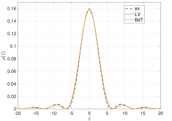
(a)

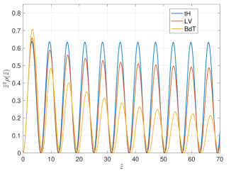
(b)

Figure 1: Plots of the resulting density, $\rho(\tilde{z})$, and $\tilde{z}^{2}\rho(\tilde{z})$ are given for all three models. The discrepancy between the models in $\rho(\tilde{z})$ is small but finite, and the $1/\tilde{z}^{2}$ asymptotic behavior is confirmed.

It is worthwhile to note that the use of current-quark masses in the ’t Hooft model causes the two different models to obtain very different masses of the first excited state. Ref Li and Vary (2021) obtains excitation energies of approximately 1 GeV and associates these values with excited states of the pion. In the present work, using modern values of the current quark masse  Zyla et al. (2020) gives the lowest excited state a mass on the order of $g$, or about 3 GeV. This is high enough into the continuum of states with large widths to be unobservable. Thus, the version of the ’t Hooft model used here preserves the spectra produced by LFHQCD.

The confining aspects of the ’t Hooft model have been well-studied long ago ’t Hooft (1974); Callan et al. (1976), using a momentum-space ($x$) dependence approach based on studying the cancellation of infrared singularities. Another, possibly more intuitive approach, may be obtaining by examining coordinate-space wave functions that depend on the canonically conjugate spatial variable, ${\tilde{z}}$. An intuitive way to think about this variable is that it is the separation between the quark and anti-quark in the direction of motion of a pion moving with high momentum.

Coordinate-space wave functions are obtained using the transformation

$$\chi({\tilde{z}})\equiv\int_{0}^{1}{dx\over\sqrt{2\pi}}e^{ix{\tilde{z}}}\chi(x).$$ (20)

It is useful to examine the density $\rho({\tilde{z}})\equiv|\chi({\tilde{z}})|^{2}$, a real-valued quantity, for the three models are shown in Fig. 1(a). These results seem very similar because of the relatively small quark masses of the three models. The densities seem to go to 0 for large absolute values of ${\tilde{z}}.$ They do, but there in an interesting feature seen by plotting ${\tilde{z}}^{2}\rho({\tilde{z}})$ in Fig. 1(b): the densities fall as $1/{\tilde{z}}^{2}$.

This behavior may be understood by making a asymptotic expansion, obtained by using $e^{i{\tilde{z}}x}=1/(i{\tilde{z}})\partial_{x}e^{i{\tilde{z}}x}$ and the feature that $\chi(x)$ vanishes at the end points. Then

$$\lim_{|{\tilde{z}}|\to\infty}\chi({\tilde{z}})={i\over{\tilde{z}}}\int_{0}^{1}{dx\over\sqrt{2\pi}}e^{ix{\tilde{z}}}\partial_{x}\chi(x).$$ (21)

Squaring this quantity leads to the stated $1/{\tilde{z}}^{2}$ dependence.

The similarity of the behaviors for small masses suggests that the chiral limit should be examined. In this case, $\chi(x)=1$ for all three models. Then a simple closed-form expression for $\chi({\tilde{z}})$ can be obtained. The resulting density, $\rho_{\chi}({\tilde{z}})$ is given by

$$\rho_{\chi}({\tilde{z}})={2\over\pi}{\sin^{2}{{\tilde{z}}/2}\over{\tilde{z}}^{2}},$$ (22)

an expression that accounts explicitly for the oscillatory behavior as well as the $1/{\tilde{z}}^{2}$ asymptotic behavior. One may also examine the spatial extent of the pion wave function by considering the mean-square value of ${\tilde{z}}^{2}$, that is given by the ground-state expectation value:

$$\langle\chi|{\tilde{z}}^{2}|\chi\rangle={2\over\pi}\int_{-\infty}^{\infty}\,dz\,\sin^{2}({\tilde{z}}/2)=\infty.$$ (23)

In the chiral limit the pion has an infinite spatial extent, true for all three models.

It is necessary to see how or if this infinite size conflicts with current understanding. First note that the elastic pion form factor of LFHQCD has already been computed using $\chi(x)=1$; see e.g. Ref. de Teramond et al. (2018). The infinite extent is buried within the integrals needed to compute the elastic form factor, a consequence the ability to probe with only transverse momentum transfers; see e.g. the review Miller (2010).

The relevance of the infinite longitudinal extent can be understood in analogy with the familiar Ioffe-time argument Gribov et al. (1965); Ioffe (1969); Kovchegov and Levin (2012); Braun and Müller (2008) for deep inelastic scattering at small values of Bjorken $x$. The idea is that an incident virtual photon fluctuates into a $q\bar{q}$ pair. The energy difference, $\Delta E$, between the two states is very small, so that the fluctuation lives for a long time $\Delta t>1/\Delta E$. For virtual photons of high energy, the extent of the fluctuation is $c\Delta t$ is very large. Now consider a high-momentum pion incident on a target. The value of $\Delta E$ goes to 0 if both the pion and its constituents are massless. Thus the infinite extent of a mass-less pion is part of standard lore.

We summarize. The similarities and differences between the three models of Refs.  De Téramond and Brodsky (2021); Li and Vary (2021); ’t Hooft (1974) are exhibited. Very significant differences in the excitation spectra, at both low and high energies, are obtained, even though all of the ground-state wave functions are the same in the chiral limit. If the ’t Hooft model is used along with current values of light-quark masses, the original spectrum calculations reviewed in Ref. Brodsky et al. (2015) are preserved. Finally, the pion is shown to have an infinite extent in the longitudinal direction.