Fast Solution Methods for Fractional Differential Equations in the Modeling of Viscoelastic Materials^†

Abstract

Fractional order models have proven to be a very useful tool for the modeling of the mechanical behaviour of viscoelastic materials. Traditional numerical solution methods exhibit various undesired properties due to the non-locality of the fractional differential operators, in particular regarding the high computational complexity and the high memory requirements. The infinite state representation is an approach on which one can base numerical methods that overcome these obstacles. Such algorithms contain a number of parameters that influence the final result in nontrivial ways. Based on numerical experiments, we initiate a study leading to good choices of these parameters.

Keywords: Fractional differential equation, fast solution, diffusive representation

1 Introduction

One of the most commonly suggested and used approaches for formulating the stress-strain relations for viscoelastic materials is based on the use of Caputo differential operators of fractional order, cf., e.g., Gerasimov [18], Caputo [5] and Dzherbashyan and his collaborators [15]. These operators are defined, for the case $0<\alpha<1$ that is of interest here, by

$$D_{*0}^{\alpha}y(t):=D_{0}^{\alpha}[y-y(0)](t)$$ (1)

where $D_{0}^{\alpha}$ is the Riemann-Liouville differential operator defined by

$$D_{0}^{\alpha}y(t):=DJ_{0}^{1-\alpha}y(t).$$ (2)

Here $D$ is the classical first order differential operator and

$$J_{0}^{\beta}y(t):=\frac{1}{\Gamma(\beta)}\int_{0}^{t}(t-s)^{\beta-1}y(s)\,\mathrm{d}s,$$ (3)

for $\beta>0$, is the Riemann-Liouville integral operator of order $\beta$. A detailed discussion of the properties of these operators may be found in [10, Chapters 2 and 3].

A typical material model that includes a few other models as special cases is the fractional Zener model or fractional standard linear solid,

$$a_{0}\sigma(t)+a_{1}D_{*0}^{\alpha}\sigma(t)=m\epsilon(t)+b_{1}D_{*0}^{\alpha}\epsilon(t),$$ (4)

where $\alpha\in(0,1)$ is a material parameter [23, 25, 22]. Depending on the type of experiment that is to be described (e.g., a creep test or a relaxation test), stress $\sigma$ may be given and strain $\epsilon$ is the unknown function or vice versa. In either case, the equation is a special case of the general mathematical formulation

$$D^{\alpha}_{*0}y(t)=f(t,y(t))$$ (5a)

where the function $$y \sigma \epsilon [0,T] \{\sigma,\epsilon\} f f y$$ (that typically corresponds to one of the functions or ) is sought on some interval whereas the other function from the set is used to define the function on the right-hand side of the fractional differential equation (5a). Under standard conditions on the function , a unique solution can be guaranteed [10, Theorem 6.5] if this differential equation is considered in combination with an initial condition of the form

$$y(0)=y_{0}$$ (5b)

with an arbitrary $$y_{0}\in\mathbb{R}$$.

An account of the historical development that has lead to such models is provided by Rossikhin and Shitikova [27, 28].

For the numerical solution of such intial value problems, many methods have been proposed; cf., e.g., [2, 11, 12, 17, 21]. A common feature of a large part of these methods is that, in order to correctly handle the non-locality of the fractional differential operators, they require a relatively large amount of time and/or computer memory [14].

A possible solution for this challenge is to introduce a so-called diffusive representation (or infinite state representation) of the fractional differential operator, cf. [26]. This is a representation of the form

$$D_{*0}^{\alpha}y(t)=\int_{0}^{\infty}\phi(w,t)\,\mathrm{d}w$$ (6a)

where the integrand $$\phi \phi(w,t) w\in(0,\infty) t$$ (whose values for are called the observed system’s infinite states at time ) solves the inhomogeneous linear first order initial value problem

$$\frac{\partial}{\partial t}\phi(w,t)=h_{1}(w)\phi(w,t)+h_{2}(w)y^{\prime}(t),\quad\phi(w,0)=0,$$ (6b)

with certain functions $$h_{1},h_{2}:(0,\infty)\to\mathbb{R}$$. Many different specific choices for these functions are admissible and have been suggested in the literature; cf., e.g., [1, 3, 6, 8, 9, 19, 20, 24, 29, 30, 31, 32, 33].

A common feature of all these special cases of diffusive representations is that using them allows to reduce the computational complexity of the fractional differential equation solver from the $O(N^{2})$ amount of a naive implementation of a classical method or the $O(N\log^{2}N)$ or $O(N\log N)$ that can be achieved by suitable modifications [13, 16, 17] to just $O(N)$. Moreover, in this way the $O(N)$ memory requirement of the standard algorithms or the $O(\log N)$ demands of some of the modified versions mentioned above is reduced to $O(1)$.

While the memory and run time requirements of such diffusive representation based algorithms are thus immediately evident, their accuracy and their convergence properties are not so obvious. Indeed, for many of the methods listed above, only a very incomplete error analysis is available. In this paper, we therefore aim to start a systematic analysis of the corresponding properties of at least one such numerical method. We believe that our findings can also be transferred to many of the other algorithms.

The core of our approach is the observation that any fractional differential equation solver needs to be based on some discretization of the associated differential operator (or the corresponding integral operator if the initial value problem is reformulated as a Volterra equation before beginning the numerical treatment). In fact, the approximation quality that this discretization can offer is decisive for the performance of the differential equation solver. Therefore, this paper will concentrate on a number of such discretizations for one specific diffusive representation of the differential operator. In view of the construction described in (6), all these discretizations essentially require two components: A numerical integration method for dealing with the integral on the right-hand side of (6a) and a numerical solver for the first order initial value problem (6b). Each of these components introduces a certain error into the final result. We shall now investigate the effects of these error components.

2 The Reformulated Infinite State Scheme

The concrete approach that we shall discuss is the relatively recent “Reformulated Infinite State Scheme” (RISS) of Hinze et al. [19]. It is based on the identity

$$D^{\alpha}_{*0}y(t) = \sin\frac{\alpha\pi}{2}\omega^{\alpha-1}y^{\prime}(t)-\int_{0}^{\infty}\mathcal{K}(\lambda)\frac{\partial}{\partial t}z(\lambda,t)\,\mathrm{d}\lambda$$

$${}+\cos\frac{\alpha\pi}{2}\omega^{\alpha}y(t)-\omega^{2}\int_{0}^{\infty}\mathcal{K}(\lambda)Z(\lambda,t)\,\mathrm{d}\lambda$$

for $t>0$ (a slight generalization of (6a)) where

$$\omega=\sqrt{\frac{2-\alpha}{\alpha}}\quad\mbox{ and }\quad\mathcal{K}(\lambda)=\frac{\sin\alpha\pi}{\pi}\frac{\lambda^{\alpha}}{\lambda^{2}+\omega^{2}}$$

and where, for $\lambda>0$, the functions $z$ and $Z$ satisfy the initial value problems

$$\frac{\partial}{\partial t}z(\lambda,t)=y^{\prime}(t)-\lambda z(\lambda,t),\quad z(\lambda,0)=0,$$ (8)

and

$$\frac{\partial}{\partial t}Z(\lambda,t)=y(t)-\lambda Z(\lambda,t),\quad Z(\lambda,0)=0,$$ (9)

respectively. For the representation (2), we shall look at a number of different concrete discretizations, starting with the original proposal of [19]. Their suggestion is to approximate the integrals over the half-line in (2) by a truncated compound Gaussian quadrature. This means that one introduces some subdivision points $0=\eta_{0}<\eta_{1}<\ldots<\eta_{K}$, writes

$$\int_{0}^{\infty}\mathcal{K}(\lambda)\zeta(\lambda,t)\,\mathrm{d}\lambda\approx\sum_{k=1}^{K}\int_{\eta_{k-1}}^{\eta_{k}}\mathcal{K}(\lambda)\zeta(\lambda,t)\,\mathrm{d}\lambda$$ (10)

(where $\zeta$ may be either $Z$ or $\frac{\partial z}{\partial t}$) and approximately computes each of the integrals on the right-hand side of (10) by a $J$-point Gauss-Legendre quadrature. The specific suggestion from [19] that we shall follow here first is to choose $J=10$, $K=25$ and $\eta_{k}=10^{-5+10(k-1)/(K-1)}$ for $k=1,2,\ldots,K$, so that the tail of the integration range which is discarded is the interval $[10^{10},\infty)$. For the approximate solution of the initial value problems (8) and (9), the authors of [19] suggest to use MATLAB’s ode15s function. This is a proposal that we shall not adopt here because ode15s may switch between different concrete ODE solvers, making a precise analysis virtually impossible. Rather, we follow the advice of [1, 9] in a similar situation and use an A-stable scheme (which may not necessarily be the case in ode15s). More specifically, we will test both the backward Euler formula (a first-order method), viz.

$$z(\lambda,t_{n})\approx\frac{1}{1+h\lambda}\left(z(\lambda,t_{n-1})+hy^{\prime}(t_{n})\right)$$ (11a)

and

$$Z(\lambda,t_{n})\approx\frac{1}{1+h\lambda}\left(Z(\lambda,t_{n-1})+hy(t_{n})\right)$$ (11b)

where $h$ is the step size, and the trapezoidal method (which is of second order),

$$z(\lambda,t_{n})\approx\frac{z(\lambda,t_{n-1})\left[1-\frac{h}{2}\lambda\right]+\frac{h}{2}[y^{\prime}(t_{n})+y^{\prime}(t_{n-1})]}{1+h\lambda/2}$$ (12a)

and

$$Z(\lambda,t_{n})\approx\frac{Z(\lambda,t_{n-1})\left[1-\frac{h}{2}\lambda\right]+\frac{h}{2}[y(t_{n})+y(t_{n-1})]}{1+h\lambda/2}.$$ (12b)

It may be observed that the kernel $\mathcal{K}$ in the integrals in (2) behaves as $\mathcal{K}(\lambda)\sim\lambda^{\alpha}$ for $\lambda\to 0$ and so, since $0<\alpha<1$, it is not differentiable at the origin. This is a situation that the compound Gauss method in its original form cannot handle very well. Therefore, we also investigate the behaviour of a slightly modified scheme where we replace the application of the Gauss-Legendre formulas to the integrals on the right-hand side of (10) by (a) the standard Clenshaw-Curtis (CC) formula [4] for those subintervals $[\eta_{k-1},\eta_{k}]$ where $\eta_{k-1}\geq 1$ (i.e. the subintervals that are sufficiently far away from the singular point of the kernel $\mathcal{K}$), and (b) a weighted Clenshaw-Curtis method with weight function $\lambda^{\alpha}$, thus accurately capturing the asymptotics of $\mathcal{K}(\lambda)$, for the remaining subintervals.

3 A Comparison of the Fundamental Variants of the Algorithm

We start by looking at the run times of the algorithm. Table 1 shows the run times required for a typical example (the results for other examples are comparable). In particular, we can see that, as expected from the construction of the algorithm, the run times are approximately proportional to $JKh^{-1}$. We can also see that the trapezoidal ODE solver, having a more complex structure than the backward Euler method (in particular, requiring more evaluations of the function $y$), usually requires a significantly longer run time (more precisely: up to almost three times as long) than backward Euler. However, we will see below that this increased run time often comes with a significant accuracy benefit that more than makes up for the higher cost.

Table 1: Run times (in seconds) for computation of $D^{\alpha}_{*0}y(t)$ for $t\in[0,3]$ with $\alpha=0.4$ and $y(t)=t^{1.6}$ (RISS, exact evaluation of $y^{\prime}$)

		backward Euler		trapezoidal
		ODE solver		ODE solver
ODE solver time step size $h$		$10^{-2^{\vphantom{2}}}$	$10^{-4}$	$10^{-2}$	$10^{-4}$
compound	$J=25$, $K=10$	0.547	57.20	1.484	148.4
Gauss	$J=10$, $K=25$	0.609	58.28	1.406	138.5
quadrature	$J=15$, $K=7$	0.297	30.22	0.453	46.0
compound	$J=25$, $K=10$	0.641	74.09	1.406	137.9
(weighted) CC	$J=10$, $K=25$	0.578	60.00	1.359	134.2
quadrature	$J=15$, $K=7$	0.266	28.05	0.453	44.1

Regarding the accuracy of the numerical results, we first refer to Figs. 1 and 2. In Fig.  1, we have looked at a rather well behaved example, viz. the computation of $D^{0.4}_{*0}y(t)$ with the differentiable function $y(t)=t^{1.6}$, for $t\in[0,3]$. We have used the RISS scheme with parameters $J=25$ and $K=10$ for the numerical quadrature. All possible combinations of quadrature formula (compound Gauss or compound CC) and ODE solver (backward Euler or trapezoidal) have been tried with different numbers of time steps in the ODE solver. Each of the four curves in that figure shows the maximal error over the entire interval for one of these four combinations. Figure 2 shows the analog results for $y(t)=t^{0.6}$ (a much less smooth function, but nevertheless a function with a behaviour that is typical for solutions to fractional differential equations), with all other parameters being the same as in Fig. 1.

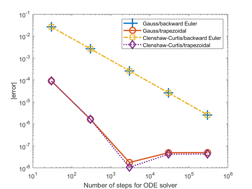
Figure 1: Maximal absolute values of approximation errors of RISS methods with different discretizations for computation of $D^{0.4}_{*0}y(t)$ with $y(t)=t^{1.6}$. In all cases, $J=25$ and $K=10$.

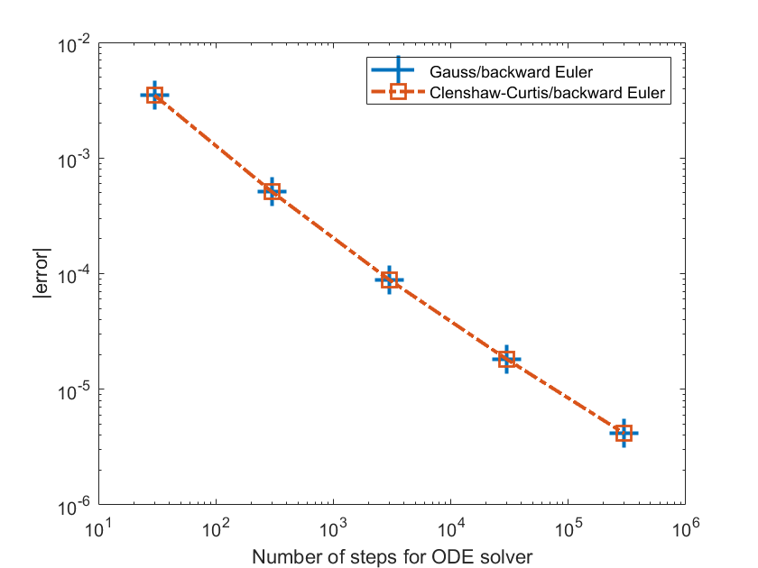
Figure 2: Maximal absolute values of approximation errors of RISS methods with different discretizations for computation of $D^{0.4}_{*0}y(t)$ with $y(t)=t^{0.6}$. In all cases, $J=25$ and $K=10$.

From these two examples, we can already observe a few properties that are also valid in general:

• The choice of the quadrature formula (compound Gauss or compound (weighted) Clenshaw-Curtis) only has a negligible effect on the final result. This may be considered to be slightly unexpected because, as indicated at the end of Section 2, the idea behind considering the (weighted) Clenshaw-Curtis scheme was that the Gauss method might not perform well. However, this observation has a natural explanation: We do not use the Gauss method in its standard form but a compound Gauss method with a highly graded mesh (the mesh grading being described by the choice of the parameters $\eta_{k}$). Such graded meshes indeed are very suitable for treating singularities of the type encountered here, and it is the influence of this mesh grading (which is the same for both choices of the quadrature formulas) that leads to this small difference between Gauss and Clenshaw-Curtis.

• The overall error that is displayed in the figure consists of two components due to the quadrature formula and the ODE solver, respectively.

• For the trapezoidal method, a certain saturation is reached when the error reaches a level of about $5\cdot 10^{-8}$. This indicates that the error of the quadrature formula (which, as indicated above, is almost exactly the same in all cases) approximately has this value. For sufficiently small step sizes, the ODE solver’s error becomes so small that the quadrature error completely dominates the overall error.

• In both examples, the overall error decreases to this level as $O(h)$ for the backward Euler method. This matches the well known fact that the backward Euler method is of first order.

• For the trapezoidal method, the decrease is $O(h^{1.6})$ in the example shown in Fig. 1. The full second order convergence that this method can have under optimal circumstances is not achieved because the function $y\notin C^{2}$.

• For the example presented in Fig. 2, we cannot directly apply the trapezoidal method because, as can be seen from (12a) for $n=1$, the approximate computation of the infinite states $z(\lambda,t_{1})$ requires the evaluation of $y^{\prime}(t_{0})=y^{\prime}(0)$ which does not exist. We shall discuss some ways to successfully deal with this challenge in Section 4.

The plots of Figs. 1 and 2 demonstrate the effects of the choice of the quadrature formula, the ODE solver and the solver’s step size as the integration range decomposition and the number of quadrature points remain unchanged. The next step of our investigation is to see what will happen when these latter parameters do change. Some results in this connection are shown in Table 2.

Table 2: Absolute values of errors for the example from Fig. 1 for different choices of $J$ and $K$

			backward Euler		trapezoidal
			ODE solver		ODE solver
time step size $h$			$10^{-2^{\vphantom{2}}}$	$10^{-4}$	$10^{-2}$	$10^{-4}$
	$J$	$K$
compound	25	10	2.63E$-$3	2.63E$-$5	1.65E$-$6	4.96E$-$8
Gauss	10	25	2.63E$-$3	2.63E$-$5	1.66E$-$6	4.43E$-$8
quadrature	15	7	2.63E$-$3	2.15E$-$5	3.17E$-$6	4.87E$-$6
compound	25	10	2.63E$-$3	2.63E$-$5	1.66E$-$6	4.24E$-$8
(weighted)	10	25	2.63E$-$3	2.63E$-$5	1.64E$-$6	6.35E$-$8
CC quadr.	15	7	2.83E$-$3	2.26E$-$4	2.01E$-$4	1.99E$-$4

The results of Table 2 indicate the following facts:

• As in the figures above, we can see that the backward Euler method induces a relatively large error that dominates the entire process. In other words, if one wants to apply this ODE solver with the step sizes used here, it is possible to significantly reduce the values of the parameters $J$ and $K$, and hence also the computational complexity, without any noticeable adverse effects on the final result.

• For the case $J=15$ and $K=7$, the compound Gauss quadrature produces significantly better results than the compound (weighted) Clenshaw-Curtis method for most choices of the ODE solver. In other examples, e.g. when the order of the derivative is changed from $0.4$ to $0.82$, the opposite can be observed. For this behaviour, no explanation is currently available.

4 A Refinement

As indicated above, it follows from eq. (12a) that the trapezoidal method can only be used as the ODE solver in the scheme under consideration if the function $y$ is differentiable throughout the entire interval of interest and, in particular, at least has one-sided derivatives at the end points of this interval. However, it is well known, cf. [10, §6.4] or [7], that this assumption is satisfied at the initial point, i.e. at the left end point of the interval in question, only in exceptional cases. Therefore, if one would like to work with the trapezoidal method in our context, then one needs to find a way to avoid the explicit use of the function $y^{\prime}$ in eq. (12a).

The most natural approach to deal with this challenge is to replace the terms $y^{\prime}(t_{n})$ and $y^{\prime}(t_{n-1})$ by appropriately chosen finite differences. To this end, we have tested a procedure that appears to be a rather natural concept. The construction of this scheme is based on exploiting the following observations:

• The expressions $y^{\prime}(t_{n})$ and $y^{\prime}(t_{n-1})$ do not appear in eq. (12a) in an independent manner; rather, only their sum is relevant.

• The reason for using the trapezoidal formula is its higher accuracy when compared to the backward Euler method. This will be lost if one uses a very rough approximation of the derivative; hence, one should use a finite difference that is second order accurate.

• In the first step, i.e. in the case $n=1$, one should only use a forward difference to approximate the term $y^{\prime}(t_{n-1})=y^{\prime}(0)$ as otherwise one would need to evaluate $y(-h)$. This clearly should be avoided because it cannot be guaranteed that $y$ is defined for negative arguments.

• For analog reasons, in the last step one should only use a backward difference for $y^{\prime}(t_{n})$.

• In all other steps, centered differences may be used.

Therefore, in the first attempt we have chosen to use the discretizations

$$y^{\prime}(t_{n})\approx\frac{1}{2h}\times\cases{(-y(t_{2})+4y(t_{1})-3y(t_{0}))&if $n=0$,\cr(3y(t_{N})-4y(t_{N-1})+y(t_{N-2}))&if $n=N$,\cr(y(t_{n+1})-y(t_{n-1}))&else,\cr}$$ (13)

in each case of which have an error of $O(h^{2})$ if $y\in C^{2}[t_{0},t_{N}]$. Even though, as mentioned above, this smoothness assumption is not satisfied in all common applications, we will nevertheless obtain results that so sufficiently accurate that their error does not dominate the error induced by the trapezoidal formula. It thus follows that our modified algorithm can be constructed by replacing the term $(h/2)[y^{\prime}(t_{n})+y^{\prime}(t_{n-1})]$ in the numerator of the right-hand side of (12a) by

$$\cases{y(t_{1})-y(t_{0})&if $n=1$,\cr y(t_{N})-y(t_{N-1})&if $n=N$,\cr(y(t_{n+1})+y(t_{n})-y(t_{n-1})-y(t_{n-2}))/4&else.\cr}$$

For the sake of consistency and to obtain even more insight, we also modify the backward Euler method in a corresponding way. Here it suffices to replace the term $hy^{\prime}(t_{n})$ in (11a) by the associated backward difference, i.e. by $(y(t_{n})-y(t_{n-1}))$, so that this method also does not require to evaluate derivatives of $y$ any more.

Figure 3 shows the numerical results for the example already discussed in Fig. 1, where now the “standard” backward Euler and trapezoidal methods given in (11a) and (12a), respectively, have been modified in the indicated manner. It can be seen that the numerical results differ from those obtained with the unmodified methods only by a very small amount. In particular, all the conclusions drawn about the behaviour of the methods for this example remain valid. This indicates that the modifications have introduced an additional error that is of the same order as the error that the respective ODE solvers induce anyway, so that the overall error order remains unchanged.

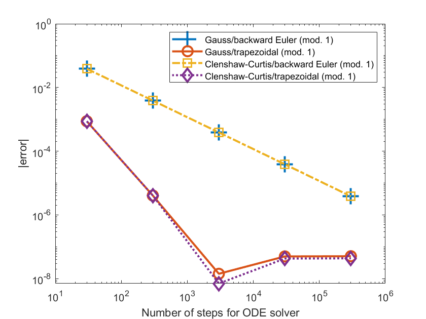
Figure 3: Maximal absolute values of approximation errors of first modified RISS methods with different discretizations for computation of $D^{0.4}_{*0}y(t)$ with $y(t)=t^{1.6}$. In all cases, $J=25$ and $K=10$.

Similarly, Fig. 4 shows the numerical results of these modified approaches for the example from Fig. 2. Here now we can see that our modification admits to use not only the backward Euler method (as before) for this example but also the modified trapezoidal algorithm which was not possible for the unmodified version. The modified backward Euler scheme still exhibits an $O(h)$ convergence towards the saturation limit induced by the quadrature formula. For the modified trapezoidal formula, the behaviour is more complex: The graphs exhibit a clearly recognizable kink. An analysis of the slopes of the graphs at either side of the kink indicate a convergence behaviour towards the saturation limit that has the form $c_{1}h^{0.6}+c_{2}h^{1.6}+o(h^{1.6})$ with some nonzero constants $c_{1}$ and $c_{2}$ having the property that $|c_{1}|$ is very much smaller than $|c_{2}|$. Therefore, while $h$ is relatively large, $c_{1}h^{0.6}$ is still much smaller in absolute value than $c_{2}h^{1.6}$, so the latter contribution dominates the entire error. When $h$ becomes smaller, the situation reverses and the graph’s slope becomes less steep.

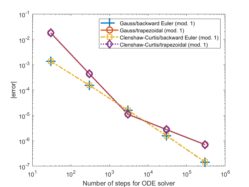
Figure 4: Maximal absolute values of approximation errors of first modified RISS methods with different discretizations for computation of $D^{0.4}_{*0}y(t)$ with $y(t)=t^{0.6}$. In all cases, $J=25$ and $K=10$.

An alternative idea in the context of the trapezoidal method is to always use a forward difference, i.e. the method used in the first case of eq. (13), to approximate the term $y^{\prime}(t_{n-1})$ in the expression $(h/2)[y^{\prime}(t_{n})+y^{\prime}(t_{n-1})]$ in (12a) and to use the backward difference from the second case in (13) to replace $y^{\prime}(t_{n})$ there. This yields the expression

$$\frac{h}{2}[y^{\prime}(t_{n})+y^{\prime}(t_{n-1})]\approx y(t_{n})-y(t_{n-1})$$

that, apart from being of a slightly simpler structure, also has the advantage that it can be used for all $n$ so that a distinction of cases is no longer necessary.

Moreover, for the backward Euler method we may also use a second order centered difference, i.e. we may replace $hy^{\prime}(t_{n})$ by $(y(t_{n+1})-y(t_{n-1}))/2$.

The numerical results obtained for our two examples with these alternative modifications are shown in Figs. 5 and 6.

For the first example, we once again find almost no difference between this approach and the original or the first modified version (see Fig. 5).

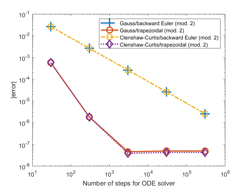
Figure 5: Maximal absolute values of approximation errors of RISS methods using second modification with different discretizations for computation of $D^{0.4}_{*0}y(t)$ with $y(t)=t^{1.6}$. In all cases, $J=25$ and $K=10$.

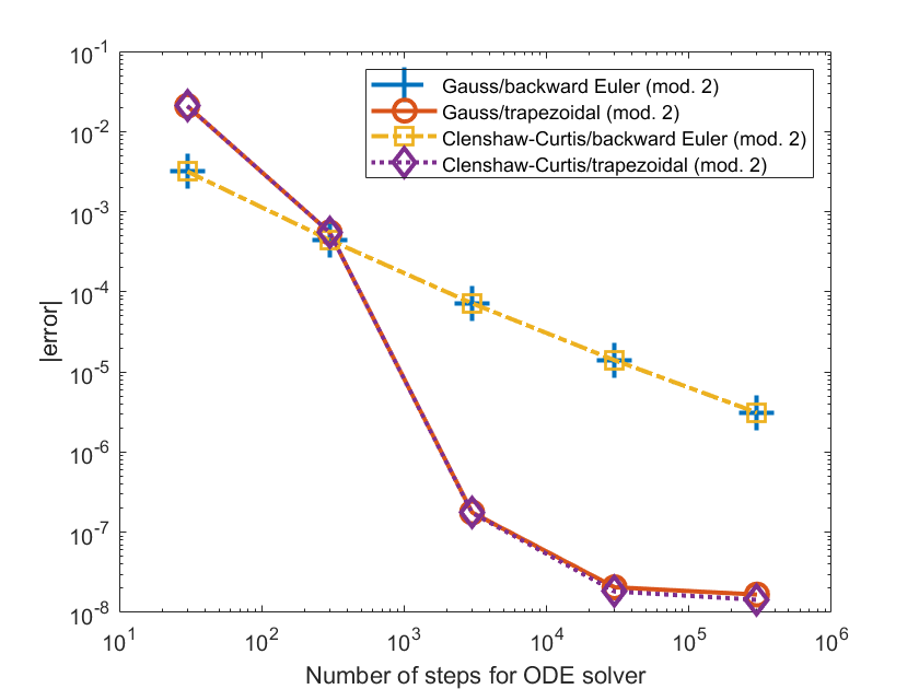
Figure 6: Maximal absolute values of approximation errors of RISS methods using second modification with different discretizations for computation of $D^{0.4}_{*0}y(t)$ with $y(t)=t^{0.6}$. In all cases, $J=25$ and $K=10$.

The second and less smooth example is shown in Fig.  6. Here, the Euler method with the second modification has a convergence order of only $O(h^{0.6})$, presumably due to the poor performance of the finite difference approximation to $y^{\prime}$ for this rather nonsmooth function. For the second modified trapezoidal method, we seem to have a simliar behaviour as in the case of the first modified version of the trapezoidal formula, i.e. an error component of the form $c_{1}h^{0.6}+c_{2}h^{1.6}+o(h^{1.6})$ with $0<|c_{1}|\ll|c_{2}|$, although the figures are a bit less clear, so a more detailed analysis should be performed.

5 Conclusion

Our numerical experiments as well as elementary theoretical considerations reveal that the error of the approximate calculation of a fractional derivative using the RISS method comprises three components and thus has the form

$$\epsilon_{1}(\eta_{K})+\epsilon_{2}(J,K,\eta_{1},\ldots,\eta_{K})+\epsilon_{3}(h).$$

Here,

• $\epsilon_{1}(\eta_{K})$ is the error due to the truncation of integration interval that behaves as $\epsilon_{3}(\eta_{K})\to 0$ for $\eta_{k}\to\infty$,

• $\epsilon_{2}(J,K,\eta_{1},\ldots,\eta_{K})$ is the integration error that satisfies$\epsilon_{2}(J,K,\eta_{1},\ldots,\eta_{K})\to 0$ if $J\cdot K\to\infty$ when $\eta_{K}$ is fixed, and

• $\epsilon_{3}(h)=O(h^{p})$ is the error due to the ODE solver where $p$ depends on choice of the solver and the degree of smoothness of function in question.

The indicated modifications of the RISS approach do not lead to any essential changes in these properties (but they may have an influence on the value of $p$ that determines the behaviour of $\epsilon_{1}(h)$).

We believe that it is possible to achieve $\epsilon_{3}=0$ by a proper choice of the quadrature formula, but the effects of this on $\epsilon_{2}$ are likely nontrivial.

Analog observations hold for almost all the other numerical methods based on such principles mentioned in Section 1.

This relatively clear general picture however needs much more detailed additional investigations to fill in details like a description of the interaction between the parameters $h$, $J$ and $K$ that might lead to some advice on which combinations of values for these parameters are useful in practice.

References

- [1] D. Baffet. A Gauss-Jacobi kernel compression scheme for fractional differential equations. J. Sci. Comput., 79:227–248, 2019.
- [2] D. Baleanu, K. Diethelm, E. Scalas, and J. J. Trujillo. Fractional Calculus—Models and numerical methods. World Scientific, Singapore, 2nd edition, 2016.
- [3] C. Birk and C. Song. An improved non-classical method for the solution of fractional differential equations. Comput. Mech., 46:721–734, 2010.
- [4] H. Braß and K. Petras. Quadrature Theory. Amer. Math. Soc., Providence, 2011.
- [5] M. Caputo. Linear models of dissipation whose is almost frequency independent—II. Geophys. J. Roy. Astron. Soc., 13:529–539, 1967.
- [6] A. Chatterjee. Statistical origins of fractional derivatives in viscoelasticity. J. Sound Vibration, 284:1239–1245, 2005.
- [7] K. Diethelm. Smoothness properties of solutions of Caputo-type fractional differential equations. Fract. Calc. Appl. Anal., 10:151–160, 2007.
- [8] K. Diethelm. An investigation of some nonclassical methods for the numerical approximation of Caputo-type fractional derivatives. Numer. Algorithms, 47:361–390, 2008.
- [9] K. Diethelm. An improvement of a nonclassical numerical method for the computation of fractional derivatives. J. Vibration Acoustics, 131:014502, 2009.
- [10] K. Diethelm. The Analysis of Fractional Differential Equations. Springer, Berlin, 2010.
- [11] K. Diethelm. Numerical methods for the fractional differential equations of viscoelasticity. In H. Altenbach and A. Öchsner, editors, Encyclopedia of Continuum Mechanics. Springer, Berlin, 2018.
- [12] K. Diethelm. Fundamental approaches for the numerical handling of fractional operators and time-fractional differential equations. In G. E. Karniadakis, editor, Handbook of Fractional Calculus with Applications, Vol. 3: Numerical Methods, pages 1–22. de Gruyter, Berlin, 2019.
- [13] K. Diethelm and A. D. Freed. An efficient algorithm for the evaluation of convolution integrals. Computers Math. Applic., 51:51–72, 2006.
- [14] K. Diethelm, V. Kiryakova, Y. Luchko, J. A. T. Machado, and V. E. Tarasov. Trends, directions for further research, and some open problems of fractional calculus. arXiv:2108.04241, 2021.
- [15] M. M. Dzherbashyan and A. B. Nersesian. Fractional derivatives and the Cauchy problem for differential equations of fractional order. Izv. Akad. Nauk. Arm. SSR, Mat., 3:3–29, 1968. (in Russian).
- [16] N. J. Ford and A. C. Simpson. The numerical solution of fractional differential equations: Speed versus accuracy. Numer. Algorithms, 26:333–346, 2001.
- [17] R. Garrappa. Numerical solution of fractional differential equations: A survey and a software tutorial. Mathematics, 6:16, 2018.
- [18] A. N. Gerasimov. A generalization of linear laws of deformation and its application to the problems of internal friction. Prikl. Mat. Mekh., 12:251–260, 1948.
- [19] M. Hinze, A. Schmidt, and R. I. Leine. Numerical solution of fractional-order ordinary differential equations using the reformulated infinite state representation. Fract. Calc. Appl. Anal., 22:1321–1350, 2019.
- [20] Ustim Khristenko and Barbara Wohlmuth. Solving time-fractional differential equation via rational approximation. arXiv:2102.05139, 2021.
- [21] C. P. Li and F. H. Zeng. Numerical Methods for Fractional Calculus. CRC Press, Boca Raton, 2015.
- [22] F. Mainardi. Fractional Calculus and Waves in Linear Viscoelasticity. World Scientific, Singapore, 2010.
- [23] F. Mainardi and G. Spada. Creep, relaxation and viscosity properties for basic fractional models in rheology. Eur. Phys. J. Spec. Topics, 193:133–160, 2011.
- [24] W. McLean. Exponential sum approximations for . In J. Dick, F. Y. Kuo, and H. Woźniakowski, editors, Contemporary Computational Mathematics, pages 911–930. Springer, Cham, 2018.
- [25] S. I. Meshkov. Description of internal friction in the memory theory of elasticity using kernels with a weak singularity. J. Appl. Mech. Tech. Phys., 84:100–102, 1967.
- [26] G. Montseny. Diffusive representation of pseudo-differential time-operators. ESAIM, Proc., 5:159–175, 1998.
- [27] Y. A. Rossikhin. Reflections on two parallel ways in the progress of fractional calculus in mechanics of solids. Appl. Mech. Reviews, 63:010701, 2010.
- [28] Y. A. Rossikhin and M. V. Shitikova. Comparative analysis of viscoelastic models involving fractional derivatives of different orders. Fract. Calc. Appl. Anal., 10:111–121, 2007.
- [29] A. Schmidt and L. Gaul. On a critique of a numerical scheme for the calculation of fractionally damped dynamical systems. Mechanics Research Communications, 33:99–107, 2006.
- [30] S. J. Singh and A. Chatterjee. Galerkin projections and finite elements for fractional order derivatives. Nonlinear Dynamics, 45:183–206, 2006.
- [31] C. Trinks and P. Ruge. Treatment of dynamic systems with fractional derivatives without evaluating memory-integrals. Computational Mechanics, 29:471–476, 2002.
- [32] L. Yuan and O. P. Agrawal. A numerical scheme for dynamic systems containing fractional derivatives. J. Vibration Acoustics, 124:321–324, 2002.
- [33] W. Zhang, A. Capilnasiu, G. Sommer, G. A. Holzapfel, and D. Nordsletten. An efficient and accurate method for modeling nonlinear fractional viscoelastic biomaterials. Comput. Meth. Appl. Mech. Engrg., 362:112834, 2020.