Suppression of thermal vorticity as an indicator of QCD critical point

Abstract

We study the impact of the QCD critical point (CP) on the spin polarization of $\Lambda$-hyperon generated by the thermal vorticity in viscous quark gluon plasma (QGP). The equations of the relativistic causal viscous hydrodynamics have been solved numerically in (3+1) dimensions to evaluate the thermal vorticity. The effects of the CP have been incorporated through the equation of state (EoS) and the scaling behavior of the transport coefficients. A significant reduction in the global polarization has been found as the CP is approached. A drastic change induced by the CP in the rapidity dependence of the spin polarization is observed which can be used as a signature of the CP.

The results from lattice quantum chromodynamics (QCD) and effective field theoretical models at non-zero temperature ($T$) and baryon chemical potential ($\mu$) reveal a rich and complex phase diagram bazavov . While at high $T$ and low $\mu$ $(\rightarrow 0)$ the quark-hadron transition is a crossover, at low $T$ and high $\mu$ the transition is of first order in nature. Therefore, it is expected that between the crossover and the first order transition there exists a point in the $\mu-T$ plane called the Critical End Point or simply the Critical Point (CP) where the first order transition ends and crossover begins Fodor:2004nz . The location of CP is not yet known from first principles lqcd , however, phenomenological studies indicate its existence stephanov . The search for the CP in the system formed in collisions of nuclei at relativistic energies is one of the outstanding problem. At present the general consensus is that the collisions of nuclei at the top Relativistic Heavy Ion Collider (RHIC) and Large Hadron Collider (LHC) energies produce QGP with small $\mu$ and high $T$ which reverts to hadronic phase via a crossover. The ongoing Beam Energy Scan - II program at RHIC and the upcoming Compressed Baryonic Matter experiment at Facility for Anti-proton and Ion Research (FAIR) and Nuclotron based Ion Collider fAcility (NICA) are planned to create system of quarks and gluons with different $\mu$ and $T$ by varying the collision energies to explore the region close to the CP. The non-monotonic variation of the fluctuations in multiplicity with collision energy in the center of mass frame ($\sqrt{s_{NN}}$) nxu , the change of sign of the fourth cumulant of order parameter with the variations of rapidity (rapidity scan)  yyin1 and beam energy stephanovprl1 , the appearance of negative sign in the kurtosis of the order parameter fluctuation near the CP stephanovprl2 are some of the proposed signals of the CP (see yyin for a review and references therein).

Relativistic hydrodynamics has been used to describe the space-time evolution of QGP and explain various experimental data quite successfully. One such crucial observable is the polarization of $\Lambda$-hyperon LambdaStar generated by the thermal vorticity during the hydrodynamic evolution of the QGP. Invigorating theoretical activities have been witnessed (see becattini2020 for a review) to understand various aspects of the polarization within the scope of hydrodynamics and transport models after the experimental measurement of the global polarization of the $\Lambda$ hyperon LambdaStar .

The magnetization of uncharged objects induced by mechanical rotation, called Barnett effect barnett and its inverse, that is, the rotation generated by varying magnetization, called the Einstein-de Haas effect deHaas originate due to the conversion between spin ($S$) and orbital angular momentum ($L$) via spin-orbit coupling constrained by the conservation of total angular momentum $\vec{J}\ (=\vec{L}+\vec{S})$. Similar kind of coupling between $L$ and $S$ in the system formed in relativistic heavy ion collision results into the spin polarization of particles. The initial orbital angular momentum (OAM) imparted by the spectators in non-central heavy ion collisions makes the fireball of QGP to rotate and polarize the quarks ztliang . This rotation may then appear as local vorticities in the fireball, the exact mechanism for which is not yet fully understood. Vorticity is a measure of the local spinning of fluid elements. The coupling of fluid vorticity and quantum mechanical spin has been experimentally demonstrated for the first time in Ref. spinhydro . Such an information is reflected in the spin polarization of final state hadrons. However, the vorticity can be generated by the viscous stresses of the system even in the absence of an initial OAM. Hence, spin polarization of hadrons has two contributions: one coming through OAM and another generated through viscosities of the system. The first contribution depends on the details of mechanism of transfer of initial OAM to vorticity and is sensitive to the initial condition. The second contribution depends on the transport properties of the system and will be sensitive to the EoS. In this letter, we focus on the second contribution and discuss about the first one in the supplemental material supplement . The goal here is to understand the CP induced change in the vorticity and its consequences on the spin polarization of $\Lambda$ hyperon. In other words if $\varpi_{\mu\nu}^{\text{CP}}$ ($\varpi_{\mu\nu}$) is the vorticity in the presence (absence) of CP then what is the value of $\Delta\varpi_{\mu\nu}=(\varpi_{\mu\nu}^{\text{CP}}-\varpi_{\mu\nu}$) and the corresponding change on the spin polarization of $\Lambda$-hyperon. We show that as the CP is approached the local vorticity and hence the polarization effect is suppressed.

The presence of CP in the EoS affects the expansion of the system due to suppression of the sound wave and divergence of some of the transport coefficients hasan . This will affect the evolution of local vorticity and hence the $\Lambda$-polarization through vorticity-spin coupling. Apart from polarization, the effect of CP on the separation of baryon and anti-baryon due to chiral vortical effect is another interesting facet cve .

Here we use natural unit $c=\hbar=k_{B}=1$ where $c$ is the speed of light in vacuum, $h=2\pi\hbar$ is the Planck’s constant and $k_{B}$ is the Boltzmann’s constant. The signature metric for flat space time is taken as $g_{\mu\nu}=\text{diag}(1,-1,-1,-1)$.

We numerically solve (3+1)-dimensional relativistic viscous causal hydrodynamics using the algorithm detailed in Ref. karpenko2014 . The code contains the effect of CP through the EoS and the scaling behavior of the transport coefficients. The initial condition and the EoS models that we use to solve hydrodynamic equations have been extensively tested by reproducing the results available in Refs. chunshen2020 and  parotto2020 respectively. The CORNELIUS code Cornelius has been used to find the constant energy-density hyper surface. Our numerical results in the absence of CP have been contrasted with the known analytical results of Ref. gubser2010 and with numerical results from other publicly available codes: AZHYDRO azhydro , MUSIC music and vHLLE karpenko2014 . The reliability of our code can be further appreciated by contrasting its output with the transverse momentum, rapidity and azimuthal angle dependence of various experimental observables (see the supplemental material supplement for details).

The relativistic hydrodynamic equations that we solve are:

$$\partial_{\mu}T^{\mu\nu}=0,$$

$$\partial_{\mu}N^{\mu}=0,$$ (1)

where $T^{\mu\nu}$ is the energy-momentum tensor and $N^{\mu}$ is the net-baryon number current. Here we work in the Landau frame of reference where the $T^{\mu\nu}$ and $N^{\mu}$ are given by

$$T^{\mu\nu} =\varepsilon\,u^{\mu}\,u^{\nu}-(p+\Pi)\Delta^{\mu\nu}+\pi^{\mu\nu},$$ (2)

$$N^{\mu} =n_{B}\,u^{\mu}+V^{\mu},$$ (3)

where $\Pi$ is the bulk pressure, $\pi^{\mu\nu}$ is the shear-stress tensor which is symmetric, traceless and orthogonal to $u^{\mu}$, $V^{\mu}(=0,\text{here})$ is the baryon diffusion 4-current and $\Delta^{\mu\nu}=g^{\mu\nu}-u^{\mu}\,u^{\nu}$. The viscous terms obey the following evolution equations,

$$u^{\alpha}\partial_{\alpha}\Pi =-\frac{\Pi-\Pi_{NS}}{\tau_{\Pi}}-\frac{4}{3}\Pi\partial_{\alpha}u^{\alpha},$$ (4)

$$\langle u^{\alpha}\partial_{\alpha}\pi^{\mu\nu}\rangle =-\frac{\pi^{\mu\nu}-\pi^{\mu\nu}_{NS}}{\tau_{\pi}}-\frac{4}{3}\pi^{\mu\nu}\partial_{\alpha}u^{\alpha},$$ (5)

where $\langle\cdot\rangle$ is defined as,

$$\langle A^{\mu\nu}\rangle=\left(\frac{1}{2}\Delta^{\mu}_{\alpha}\Delta^{\nu}_{\beta}+\frac{1}{2}\Delta^{\nu}_{\alpha}\Delta^{\mu}_{\beta}-\frac{1}{3}\Delta^{\mu\nu}\Delta_{\alpha\beta}\right)A^{\alpha\beta},$$

$\Pi_{NS}$ and $\pi_{NS}^{\mu\nu}$ are the Navier-Stokes limit of $\Pi$ and $\pi^{\mu\nu}$ respectively, given by

$$\Pi_{NS}=-\zeta\theta\quad,\quad\pi_{NS}^{\mu\nu}=2\eta\left\langle\partial^{\alpha}u^{\beta}\right\rangle.$$ (6)

The coefficients of shear ($\eta$) and bulk ($\zeta$) viscosities are positive, i.e. $\eta,\zeta>0$.

The hydrodynamical equations are solved in $(\tau,x,y,\eta_{s})$ coordinates where, $\tau=\sqrt{t^{2}-z^{2}}$ and $\eta_{s}=\text{tanh}^{-1}(z/t)$. The space-time evolution begins at time $\tau_{0}$. For lower energies the initial time, $\tau_{0}$ is taken as the time required by the nuclei to pass through one other ($\sim\frac{2R}{\gamma_{z}v_{z}}$) and for higher energies ($\sqrt{s_{NN}}\geq 62.4$ GeV), $\tau_{0}=1$ fm as shown in Table  1. The initial energy density profile at $\tau_{0}$ is taken as:

$$\varepsilon(x,y,\eta_{s};\tau_{0})=e(x,y)\,f(\eta_{s}).$$ (7)

A symmetric rapidity profile, $f(\eta_{s})$, with the local energy-momentum conservation puts a constraint on $e(x,y)$ as shown in Ref. chunshen2020 . The energy deposited in the transverse plane, $e(x,y)$ depends on the number of wounded nucleons per unit area which has been calculated by using the optical Glauber model for given impact parameter ($b$) at different $\sqrt{s_{NN}}$. The quantity, $e(x,y)$ is related to the the number of wounded nucleons per unit area in the transverse plane, $n_{A}(x,y)$ and $n_{B}(x,y)$ of the colliding nuclei A and B respectively as: $e(x,y)\propto\sqrt{n_{A}^{2}+n_{B}^{2}+2n_{A}n_{B}\text{cosh}(2y_{\tt beam})}$, where $y_{\tt beam}=\text{cosh}^{-1}(\sqrt{s_{NN}}/2)$. Here we consider Au+Au collisions at $b=5.6$ fm for different $\sqrt{s_{NN}}$ that corresponds to 15-25% centrality supplement . The thickness function of the Au nucleus has been calculated by assuming Woods-Saxon profile for nuclear density with nuclear radius, $R_{0}=6.37$ fm, and surface thickness, $\delta=0.535$. The p+p inelastic cross-section, $\sigma^{\texttt{in}}_{NN}(\sqrt{s_{NN}})$, needed for the calculation of the number of wounded nucleons in the Glauber model has been taken from Refs.  sigmaNN_parametrization1 ; sigmaNN_parametrization2 .

The initial velocity profile is taken as:

$$u^{\mu}(x,y,\eta_{s};\tau_{0})=\left(\cosh(\eta_{s}),0,0,\sinh(\eta_{s})\right),$$ (8)

The initial density profiles for energy and net baryon number have been computed with the parameters used in Ref. chunshen2020 . The viscous terms have been initialized with their corresponding Navier-Stokes limit.

Table 1: Values of $\tau_{0}$ used at different colliding energies

$\sqrt{s_{NN}}$ (GeV)	14.5	19.6	27	39	62.4	200
$\tau_{0}$ (fm)	2.2	1.8	1.4	1.3	1.0	1.0

The EoS parotto2020 employed here to solve the hydrodynamic equations reproduces the lattice QCD results at zero baryon chemical potential. The parameters $w$, $\rho$ and $\alpha_{1}$ that appear in the linear mapping from Ising model to QCD in Ref. parotto2020 have been fixed as $w=1$, $\rho=2$ and $\alpha_{1}=3.85^{\tt o}$. The other parameters are same as Ref. parotto2020 . The transport coefficients are expected to diverge near the critical point following a scaling behavior amonnai :

$$\zeta\sim\xi^{3}\quad,\quad\eta\sim\xi^{0.05}.$$

where $\xi(\mu,T)$ is the equilibrium correlation length, which is obtained through mapping QCD to 3D Ising model in the critical region. In the Ising model, $\xi$ is computed by taking the derivative of equilibrium magnetization, $M(r,h)$, with respect to the magnetic field, $h$, at fixed $r=(T-T_{c})/T_{c}$, as amonnai

$$\xi^{2}=\frac{1}{H_{0}}\left(\frac{\partial M}{\partial h}\right)_{r},$$

where $H_{0}$ is a dimensionful parameter to get the correct dimensions of $\xi$. We shall take $H_{0}=1$ in our calculations and $\left(\frac{\partial M}{\partial h}\right)_{r}$ is obtained from the EoS model parotto2020 using chain rule of differentiation. The extent of the critical domain in the $\mu-T$ plane is determined by the condition: $\xi(\mu,T)=\xi_{0}$, where $\xi_{0}$ is taken as 1.75 fm. The possibility of divergent behavior is incorporated through the following expressions of the transport coefficients amonnai

$$\zeta=\zeta_{0}\left(\frac{\xi}{\xi_{0}}\right)^{3}\ ,\ \eta=\eta_{0}\left(\frac{\xi}{\xi_{0}}\right)^{0.05}$$ (9)

Outside the critical region the values of the shear and bulk viscosities denoted by $\eta_{0},\ \zeta_{0}$ respectively are chosen as denicol2018 ; denicol2014 :

$$\eta_{0}(\mu,T) =C_{\eta}\left(\frac{\varepsilon+p}{T}\right)\quad,\quad\zeta_{0}(\mu,T)=15\ \eta_{0}\left(\frac{1}{3}-c_{s}^{2}\right)^{2}$$

The above parametrization is consistent with the estimates of the temperature-dependent specific shear and bulk viscosity extracted using Bayesian method bernhard away from the critical region. The authors of Ref. Martinez compute the critical contribution to the bulk viscosity which is an order of magnitude less than that of the noncritical contribution. The effect of reduced $\zeta_{0}$ in the critical region has been discussed in supplement .

The dependence of the relaxation times appeared in Eqs.(4) and (5) on $\xi$ are parameterized as:

$$\tau_{\pi}=\tau^{0}_{\pi}\left(\frac{\xi}{\xi_{0}}\right)^{0.05}\quad,\quad\tau_{\Pi}=\tau^{0}_{\Pi}\left(\frac{\xi}{\xi_{0}}\right)^{3}.$$ (10)

where $\tau^{0}_{\pi}$ and $\tau^{0}_{\Pi}$ are the relaxation times outside the critical region which are given by denicol2018 ; denicol2014 ,

$$\frac{\tau^{0}_{\pi}}{5}=\tau^{0}_{\Pi}=\frac{C_{\eta}}{T}$$

with $C_{\eta}=0.08$.

Figure 1: Trajectories traced by the center of the fireball i.e. $x=y=\eta_{s}=0$ in the $\mu-T$ plane for different $\sqrt{s_{NN}}$. The critical point is indicated by solid black dot at $(\mu,T)=(350,143.2)$ MeV.

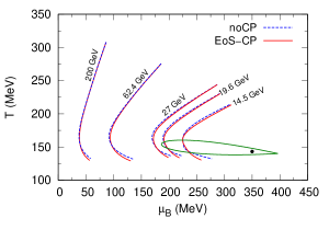
The critical region and the trajectories traced by the center of the fireball in the ($\mu-T$) plane at different $\sqrt{s_{NN}}$ are shown in Fig. 1. The black dot indicates the location of the CP at $(\mu_{c},T_{c})=(350\text{MeV},143.2\text{MeV})$ parotto2020 . The trajectories have been calculated by solving the hydrodynamic equations with (denoted by EoS-CP) and without (noCP) the effects of CP. The CORNELIUS code is then used to find the freeze-out hyper surface $\Sigma_{\varepsilon}$, defined by $\varepsilon=0.3\text{GeV}/\text{fm}^{3}$. The spin polarization has been evaluated on this hyper surface. The trajectories for $\sqrt{s_{NN}}=$14.5 GeV and 19.6 GeV pass through the critical domain (shown by the closed contour in Fig. 1) and those for higher $\sqrt{s_{NN}}$ remain outside the critical domain. We evaluate the thermal vorticity and subsequently the polarization of $\Lambda$ for system evolving along trajectories passing through both inside and outside the critical domain. The effect of the CP on the polarization is expected to be larger for $\sqrt{s_{NN}}=14.5$ GeV as the trajectory for this case is closer to the CP compared to other values of $\sqrt{s_{NN}}$ considered here.

The thermal vorticity at any space-time point of the fluid is given by Becattini1 ; Becattini2 :

$$\varpi_{\mu\nu}=\frac{1}{2}\left[\partial_{\nu}\beta_{\mu}-\partial_{\mu}\beta_{\nu}\right]$$ (11)

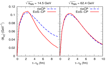
where $\beta_{\mu}=u_{\mu}/T$. The time evolution of the $x\eta$ component of the thermal vorticity, averaged over the spatial coordinates and weighted by the energy density, with and without the effects of CP are shown in Fig. 2. Initially the system has zero vorticity. The vorticity generated by the viscous effects increase at first to attain some maximum value and then decreases subsequently. The evolution of the vorticity is affected by several factors. The hydrodynamic expansion does not create or destroy vortices but reduces it through redistribution. The shear viscous coefficient is responsible for its diffusion and the stretching and baroclinic torque enhance the vorticity. Near the CP, absorption of sound wave affects the expansion directly and the diverging nature of the transport coefficients reduces the vorticity as seen in Fig. 2. The observed suppression of the vorticity due to CP at $\sqrt{s_{NN}}=14.5$ GeV is expected to influence some of the experimental results. As the evolution trajectory for $\sqrt{s_{NN}}=62.4\text{GeV}$ (and higher energies) remain outside the critical domain the results with and without the CP essentially overlap.

Figure 2: Time evolution of the mean of the $x\eta$-component of thermal vorticity for $\sqrt{s_{NN}}=14.5\text{GeV}$ and $62.4\text{GeV}$.

The local thermal vorticity and the $\Lambda$-polarization is calculated by using the following expression for mean spin vector of a spin-1/2 particle with four-momentum $p_{\nu}$ Smu as,

$$S^{\mu}(x,p)=-\frac{1}{8m}(1-n_{F})\epsilon^{\mu\nu\rho\sigma}p_{\nu}\varpi_{\rho\sigma}(x)+O(\varpi)^{2}$$

where $m$ is the mass of the particle, $\epsilon^{\mu\nu\rho\sigma}$ is the Levi-Civita tensor and $n_{F}$ is the Fermi-Dirac distribution. Since the mass of the $\Lambda$ is much larger than the temperature range being considered in this study, we assume that $1-n_{F}\approx 1$ and $n_{F}\approx n_{B}$, where $n_{B}$ is the Boltzmann distribution. Consequently the expression for the mean spin vector becomes

$$S^{\mu}(x,p)=\frac{1}{8m}\epsilon^{\mu\nu\rho\sigma}p_{\nu}\partial_{\rho}\beta_{\sigma}$$

In the rest frame of the particle, the spin vector is $S^{*\mu}=(0,{\bf{S}^{*}})$, which is obtained by using the Lorentz transformation as:

$${\bf{S}^{*}}={\bf{S}}-\frac{{\bf{p}}.{\bf{S}}}{E(E+m)}{\bf{p}}$$

The mean spin averaged over the surface $\Sigma$ is then given by Becattini1 ,

$$S^{\mu}(p)=\frac{\int d\Sigma_{\lambda}p^{\lambda}\ e^{-\beta(p.u-\mu)}S^{\mu}(x,p)}{\int d\Sigma_{\lambda}p^{\lambda}\ e^{-\beta(p.u-\mu)}}$$ (12)

The net spin is obtained by integrating over azimuthal angle ($0\leq\phi<2\pi$), rapidity ($|y|<1$) and transverse momentum ($0<p_{T}<3\text{ GeV}$) following the procedure of Ref. wu2019 . Finally the spin polarization of $\Lambda$ is given by,

$${\bf{P}}=2{\bf{S}^{*}}$$

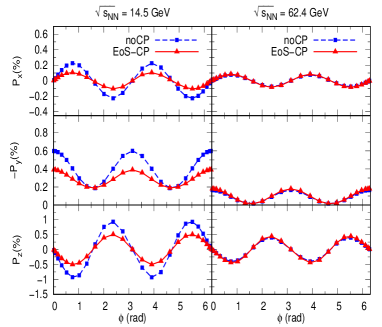
In view of an ongoing puzzle on the issue of the variation of the longitudinal polarization with azimuthal angle ($\phi$) ( signpuzzle1 ; signpuzzle2 ; STARlambda ), we display the variation of the different components of the polarization, $P_{x}$, $P_{y}$ and $P_{z}$ with $\phi$ in Fig. 3 for $\sqrt{s_{NN}}=14.5$ GeV and 62.4 GeV with and without the effects of CP. A systematic suppression of the polarization is observed ($xz$ is the reaction plane and $y$-axis is the axis of rotation here) at $\sqrt{s_{NN}}=14.5$ GeV which originates from several competing factors like enhancement of various transport coefficients, slower expansion, changes in baroclinic torque and vortex stretching near the CP. The polarization with and without the effect of CP overlap at $\sqrt{s_{NN}}=62.4$ GeV which is obvious as the trajectory for this case remains outside the critical region (Fig. 1).

Figure 3: $x$, $y$ and $z$ components of $\Lambda$-polarization are plotted respectively in the upper, middle and the lower panels as a function of azimuthal angle in momentum space for $\sqrt{s_{NN}}=14.5\text{GeV}\,\,\text{and}\,\,62.4\text{GeV}$.

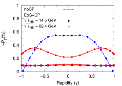
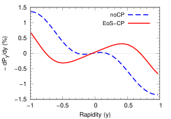
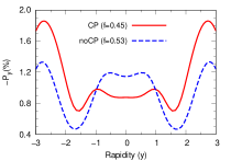
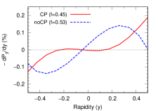
The variation of the $y$-component of the spin-polarization with rapidity ($y$) has been displayed in Fig. 4. A drastic change is induced by the CP in the rapidity distribution of spin-polarization at $\sqrt{s_{NN}}=14.5$ GeV. At $\sqrt{s_{NN}}=62.4$ GeV, the $P_{y}$ with and without CP is identical as expected. It is intriguing to note that the CP not only reduces the polarization around mid-rapidity but also introduces strong qualitative changes in the slopes of the curves as shown in Fig. 5.

Figure 4: $y$-component of $\Lambda$-polarization plotted as a function of momentum rapidity for $\sqrt{s_{NN}}=14.5\,\,\text{GeV}\,\,\text{and}\,\,62.4\text{GeV}$.

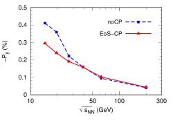
Finally, on integration over $p_{T}$, $\phi$ and $y$ the global polarization is obtained as a function of $\sqrt{s_{NN}}$. The suppression of polarization is conspicuous for the trajectories passing through the critical domain at lower $\sqrt{s_{NN}}$ (Fig. 6). The slope of the curve without CP is much steeper than the one with CP at lower $\sqrt{s_{NN}}$. We have taken the initial orbital angular momentum (OAM) of the fireball as zero resulting in smaller polarization compared to experimental value LambdaStar . Inclusion of OAM through the non-zero initial value of the velocity profile Becattini1 will enhance the magnitude of $-P_{y}$, however, the difference in the polarization observed here with and without CP will still persist. Results with the inclusion of OAM have been discussed in the supplemental material supplement . The sensitivity of this result on other parameters has also been presented in the supplemental material supplement .

Figure 5: Negative slope of the $y$-component of the polarization of $\Lambda$-hyperon plotted as a function of rapidity.

Figure 6: Global polarization of $\Lambda$-hyperon plotted as a function of $\sqrt{s_{NN}}$.

Conclusions - It is well-known that the local vorticity of the fluid couples with the quantum mechanical spin of the particles and polarize them. We have evaluated the spin polarization of $\Lambda$-hyperon with and without the effects of CP and found a strong change in the spin polarization around mid-rapidity as the system approaches the CP. The thermal vorticity and consequently the polarization of the $\Lambda$ hyperon for different colliding energies have been estimated and found to be suppressed as the CP is approached. There are various physical processes which collectively contribute to the suppression. Although we have solved the relativistic equation to estimate the vorticity, we consider below the evolution equation for kinematic vorticity ($\vec{\omega}=\nabla\times\vec{v}$) for a compressible fluid with constant $\zeta$ and $\eta$ in the non-relativistic limit because in this form contributions from various terms appear clearly,

$$\frac{\partial\vec{\omega}}{\partial t} =\left(\vec{\omega}\cdot\vec{\nabla}\right)\vec{v}-\left(\vec{v}\cdot\vec{\nabla}\right)\vec{\omega}-\theta\vec{\omega}+\frac{1}{\rho^{2}}\vec{\nabla}\rho\times\vec{\nabla}p$$

$$-\frac{1}{\rho^{2}}\left(\zeta+\frac{1}{3}\eta\right)\vec{\nabla}\rho\times\vec{\nabla}\theta-\frac{\eta}{\rho^{2}}\vec{\nabla}\rho\times\nabla^{2}\vec{v}+\frac{\eta}{\rho}\nabla^{2}\vec{\omega}.$$

Here $\rho$ denotes the density of fluid and $\theta=\nabla\cdot\vec{v}$. As $\theta$ is a measure of the expansion of the system, a larger expansion results in smaller vorticity as suggested by the negative sign of the term $\theta\vec{\omega}$. The terms depending on transport coefficients only, are written in the second line of the above equation. The term proportional to $\nabla^{2}\vec{\omega}$ is responsible for diffusion of vorticity in space, the diffusion coefficient being $\frac{\eta}{\rho}$. The term of particular interest is proportional to $\vec{\nabla}\rho\times\vec{\nabla}\theta$ which suggests that the vorticity dissipates if there is a gradient in expansion rate for fluid cells i.e. the fluid cells having less density and expanding faster will oppose the vorticity of the denser fluid cells expanding slowly. The strength of this effect is proportional to $\left(\zeta+\frac{1}{3}\eta\right)$. It is clear that the suppression of vorticity and hence polarization, is a combined effect of the absorption of sound wave and the enhancement of various transport coefficients in presence of CP. The drastic qualitative and quantitative changes induced by CP in the rapidity distribution of $P_{y}$ can be used to detect the CP experimentally as the polarization of $\Lambda$ has already been measured by STAR collaboration LambdaStar . It is important to mention at this point that the effects of CP on the $p_{T}$ spectra of the hadrons and on the $p_{T}$ and $y$ dependence of directed and elliptic flow are found to be small singh2022 .

Some comments on the application of hydrodynamics near the CP are in order here. Near the CP, the fluctuating modes do not relax faster than the timescale of changes in slow/conserved variables due to which the local thermal equilibrium is not maintained making hydrodynamics inapplicable. The validity of the hydrodynamics can, however, be extended by adding a scalar variable representing the slow non-hydrodynamic modes connected to the relaxation rate of the critical fluctuation (see  yin and stephanov2018 for details). It has been explicitly shown that the modes associated with the scalar variable lags behind the hydrodynamic modes resulting in back reactions on the hydrodynamic variables rajagopal . Further, it has been demonstrated in Ref. rajagopal that the back reaction has negligible effects on the hydrodynamic variables. In view of this, the results presented in this work will be useful in detecting the CP. Moreover, we may also recall that if a system is not too close to CP then hydrodynamics can still be applied in a domain around the CP Stanley .

We thank Sandeep Chatterjee and Tribhuban Parida for helpful discussions regarding the UrQMD transport code.

I Supplementary Material

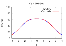
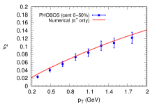
In this supplemental material, we present a few test results from our hydrodynamic code with the inclusion of the effects of critical point (CP) through the equation of state (EoS) and scaling behaviour of transport coefficients, and contrast the results without CP (denoted as noCP in the text and figures). We shall also discuss the effect of non-zero orbital angular momentum (OAM) on our results. We have already shown a comparison of our numerical results with the analytical Gubser solution in (2+1) dimensions in Ref. singh2022 . There is no analytical result available in (3+1)-dimensions. Therefore, to test the code, we compare our result on the rapidity distribution of positively charged pion with the output of publicly available MUSIC code musiccode without the resonance decays in Fig. 7. For the next check, we reproduce the PHOBOS data on $p_{T}$ dependence of elliptic flow in 0-50% centrality of Au+Au collisions at $\sqrt{s_{NN}}=200$ GeV phobos2005 in Fig. 8.

Figure 7: The comparison of the rapidity distribution of $\pi^{+}$ from our code and the publicly available MUSIC code.

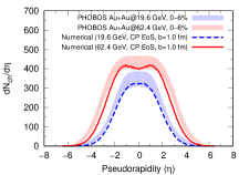
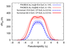
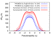
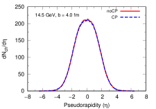
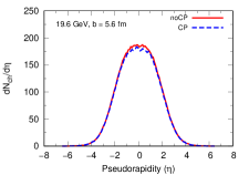
We next reproduce the charged particle pseudorapidity distribution for two colliding energies ($\sqrt{s_{NN}}$) and different centralities in Fig. 9. To generate the plots in Fig. 9, we use the switching energy density $\varepsilon_{\text{sw}}=0.3$ GeV/fm³. The constant energy density hypersurface ($\varepsilon_{\text{sw}}$) is obtained using the CORNELIUS code cornelius which is then given as input to the UrQMD transport code urqmd (which does not include spin effects) and generate 1000 events. It should be mentioned here that the width of the experimental distribution is slightly underestimated because we have used a single impact parameter and not an event-by-event simulation that would consist of a mixture of several impact parameters. The results of Fig. 9 include the effects due to CP. However, on comparing with the results without CP, the effect is negligible as demonstrated in Fig. 10 (see also Ref. singh2022 ).

Figure 8: Our numerical result on $p_{T}$ dependence of elliptic flow, $v_{2}$, compared to the experimental data from Ref. phobos2005 .

Now we implement a non-zero OAM in the initial condition. The initial condition model that we use from Ref. shen2020 has been generalized to include a non-zero OAM in Ref. shen2021 . This is done by introducing a parameter, $f$, that takes value in the interval [0,1] and it controls the fraction of longitudinal momentum that can be attributed to the flow velocity. $f=0$ corresponds to the Bjorken flow scenario. The assumption for the initial energy-momentum current in Ref. shen2021 can be achieved through the following choice of rest frame quantities:

$$p =\varepsilon\ ,\ u^{x}=u^{y}=0,$$

$$u^{\tau} =\cosh\left(\frac{y_{L}}{2}\right)\ ,\ u^{\eta}=\frac{1}{\tau_{0}}\sinh\left(\frac{y_{L}}{2}\right),$$

where $p$, $\varepsilon$, and $u^{\mu}$, respectively, denote the pressure, the energy density, and the fluid four flow-velocity. Also, $y_{L}=fy_{\text{CM}}$ denotes the local longitudinal rapidity variable and $y_{\text{CM}}$ is the local center-of-mass rapidity variable (defined in the main article). The components of the initial energy-momentum tensor then take the following form:

$$T^{\tau\tau} =(\varepsilon+p)(u^{\tau})^{2}-p=\varepsilon\cosh(y_{L}),$$

$$T^{\tau\eta} =(\varepsilon+p)u^{\tau}u^{\eta}=\frac{\varepsilon}{\tau_{0}}\sinh(y_{L}),$$

$$T^{\eta\eta} =(\varepsilon+p)u^{\eta}u^{\eta}=\frac{\varepsilon}{\tau_{0}^{2}}\cosh(y_{L}),$$

which is consistent with the assumption of Ref. shen2021 .

Figure 9: The numerical result for $dN_{\text{ch}}/d\eta$ is compared with experimental data by PHOBOS in different centralities phobos2003 ; phobos2006 .

Figure 10: $dN_{\text{ch}}/d\eta$ shown as a function of pseudorapidity with (CP) and without (noCP) the critical point in EoS for colliding energies (left) 14.5 GeV at impact parameter $b=4$ fm, and (right) 19.6 GeV at impact parameter $b=5.6$ fm.

The trace of the energy-momentum tensor is given by

$$T^{\mu}_{\mu}=T^{\tau\tau}-\tau^{2}T^{\eta\eta}=0.$$

Hence, our choice for the rest frame quantities does not violate the condition for the trace of the energy-momentum tensor. The viscous stresses are initialized to their corresponding Navier-Stokes limit, the expressions of which are:

$$\pi^{\tau\tau} =-2\eta\tau u^{\tau}(u^{\eta})^{2}-\frac{2\eta}{3\tau}u^{\tau}\left[1-(u^{\tau})^{2}\right],\ \pi^{\tau x}=-\eta\partial_{x}u^{\tau},$$

$$\pi^{\tau y} =-\eta\partial_{y}u^{\tau},\ \pi^{\tau\eta}=-\eta\tau(u^{\eta})^{3}-\frac{\eta u^{\eta}}{\tau}-\frac{\eta}{3\tau}(u^{\tau})^{2}u^{\eta},$$

$$\pi^{xx} =\frac{2\eta}{3\tau}u^{\tau},\ \pi^{xy}=0,\ \pi^{x\eta}=-\eta\partial_{x}u^{\eta},\ \pi^{yy}=\frac{2\eta}{3\tau}u^{\tau},$$

$$\pi^{y\eta} =-\eta\partial_{y}u^{\eta},\ \pi^{\eta\eta}=-\frac{4\eta}{3\tau}u^{\tau}\left[\frac{1}{\tau^{2}}+(u^{\eta})^{2}\right]$$

It was stated in Ref. shen2021 that the parameter $f$ has negligible effects on most of the global observables such as the pseudorapidity distributions, particle yields, and elliptic flow. We have checked this and conclude the same. The rest of the analysis that follows is carried out on a constant energy density hypersurface, $\varepsilon=0.3$ GeV/fm³, we shall denote this surface as $\Sigma_{\varepsilon}$ below.

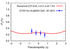
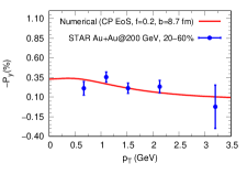
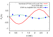
By setting $f=0.2$, impact parameter, $b=8.7$ fm, and using the same set of values for other parameters of the IC model for Au+Au collision at $\sqrt{s_{NN}}=200$ GeV, described in the main article, we compute the negative $y$-component of global polarization, $-P_{y}$, of $\Lambda$-hyperon for 20-60% centrality. Our result is $-P_{y}$=0.254%. The corresponding experimental value from STAR is 0.277$\pm$ 0.040 (stat) and using the updated PDG value of $\alpha_{\Lambda}$ is 0.243$\pm$ 0.035% (stat) star2018 . We also show the pseudorapditiy and transverse momentum dependence in the same centrality in Figs.11 and 12. Again, we use EoS with CP to generate these results. Because the difference between CP and noCP equation of states is negligible at such large colliding energy. The azimuthal angle dependence of the longitudinal component of the spin-polarization, $P_{z}$, is shown in Fig. 13. The sign of our numerical results is opposite to that of experimental data. This problem is known as the longitudinal sign puzzle in the literature (see becattini2020 for a review).

Figure 11: The numerical result for $y$-component of $\Lambda$-polarization as function of pseudorapidity is compared with the experimental data by STAR from Au+Au collisions at $\sqrt{s_{NN}}=200$ GeV in 20%-60% centrality star2018 . Vertical lines are the statistical uncertainties only.

Figure 12: The numerical result for $y$-component of $\Lambda$-polarization as function of transverse momentum ($p_{T}$) is compared with the experimental data by STAR from Au+Au collisions at $\sqrt{s_{NN}}=200$ GeV for 20-60% centrality star2018 . Vertical lines are the statistical uncertainties only.

Having validated our code we now carry out our simulation near the critical point at colliding energy $\sqrt{s_{NN}}=14.5$ GeV. The negative $y$-component of the global polarization is suppressed in the presence of CP as compared to the case when the CP is absent for a given value of $f$. This illustrates that the values of global polarization with and without CP are different at fixed $f$ which is clearly observed in the main article (Fig. 5) for zero initial OAM (corresponding to $f=0$). We carry out an exercise to verify whether the same global polarization of $\Lambda$ hyperon can be obtained with and without CP by tuning the parameter $f$ in the presence of OAM. The values $f=0.45$ with CP and $f=0.53$ without CP corresponds to the same value of $-P_{y}$=0.92% of $\Lambda$-hyperon for $b=5.6$ fm which nearly reproduces the experimental value measured by the STAR collaboraion for 20%-60% centrality. This indicates that the data on global polarization can not be used to exclusively determine the CP effects, because other parameters can be tuned to the data.

Figure 13: Azimuthal angle dependence of $z$-component of spin polarization of $\Lambda$-hyperon. STAR measurements are from Ref.star2019 .

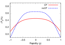
However, once the value of $f$ is tuned to the global polarization data then the use of the same value of $f$ (which fixes the OAM) predicts significant difference in the rapidity distribution of $P_{y}$ with and without CP, clearly indicating that the rapidity distribution of $-P_{y}$ is sensitive to CP. We plot the rapidity distribution of $-P_{y}$ in the top panel of Fig. 14. We observe a suppression of about $25\%$ in $-P_{y}$ at mid-rapidity. The change in other observables like $p_{T}$ spectra, elliptic flow, $dN_{\text{ch}}/dy$ is at most 8% on the surface $\Sigma_{\varepsilon}$ singh2022 . We also compute the derivative of $P_{y}$ with respect to rapidity and plot as a function of rapidity in the bottom panel of Fig. 14. We observe a slight negative slope for $-dP_{y}/dy$ at mid-rapidity opposite to the case when there is no critical point. We cannot confirm the negative sign of the slope by further approaching the critical point due to the limitations of the EoS model which is valid for $\mu_{B}<450$ MeV. Beyond 450 MeV, the speed of sound starts to give unphysical results. So close to CP, many fluid cells whose trajectories cross $\mu_{B}=450$ MeV become problematic. However, it should be mentioned that the suppression that we observe is when the center of the fireball created in $\sqrt{s_{NN}}=14.5$ GeV energy is still 100 MeV away from the critical point along the $\mu_{B}$ axis. We expect the effect to get enhanced on further approach toward the critical point.

Figure 14: The top panel shows rapidity dependence of $y$ component of $\Lambda$-hyperon polarization at $\sqrt{s_{NN}}=14.5$ GeV and $b=5.6$ fm with (CP) and without (noCP) critical point EoS, and the bottom panel shows the derivative as a function of rapidity.

The sensitivity of the spin polarization to the EoS can be understood from the following expression for the spin polarization in the rest frame of $\Lambda$-hyperon at any point on $\Sigma_{\varepsilon}$ becattini2020 :

$$\vec{S}^{*}(x,p)\propto\frac{\gamma}{T^{2}}\vec{v}\times\nabla T+\frac{1}{T}\left(\vec{\omega}-(\vec{\omega}\cdot\vec{v})\vec{v}\right)+\frac{1}{T}\gamma\vec{A}\times\vec{v},$$

where $\vec{\omega}$ is the vorticity ($=\nabla\times\vec{v}$), $\gamma$ is the Lorentz factor and $A$ denotes the acceleration of the fluid element. In nutshell, spin polarization depend on the gradients of temperature and curl of flow-velocity $(=\omega$). These gradients in turn depend on the expansion dynamics of the system and the expansion is strongly influenced by the speed of sound which is obtained from EoS. Since the sound wave gets suppressed at the critical point, the system undergoes a slow expansion that results into smaller gradients of temperature and flow-velocity, as they will not change much. This should then result into a suppression of spin-polarization as confirmed by our simulations. The effects of CP on other observables have been presented in Ref. singh2022 by solving the same hydrodynamic equations with and without the critical point.

Figure 15: Suppression in $y$-component of spin polarization for $f=0$, $\zeta^{\prime}_{0}=\zeta_{0}/10$ and $\xi^{\prime}_{0}=0.8$ fm.

To further demonstrate the robustness of our prediction, we show in Fig. 15 the suppression in polarization when the bulk viscosity away from critical region, denoted by $\zeta_{0}$ in Eq.(9) of main article, is decreased by a factor of 10 i.e. $\zeta^{\prime}_{0}=\frac{\zeta_{0}}{10}$ and the length scale, $\xi_{0}$ in Eq.(9) of main article, that marks the boundary of the critical region is taken as $\xi^{\prime}_{0}=0.8$ fm. We still see a suppression of about 30% at mid-rapidity.

References

- (1) A. Bazavov, F. Karsch, S. Mukherjee and P. Petreczky (USQCD Collaboration), arXiv:1904.09951 [hep-lat].
- (2) Z. Fodor and S. Katz, JHEP 04, 050 (2004).
- (3) H. T. Ding, F. Karsch and S. Mukherjee, Int. J. Mod. Phys. E 24, 1530007 (2015).
- (4) M. A. Stephanov, K. Rajagopal and E. V. Shuryak, Phys. Rev. Lett. 81, 4816 (1998).
- (5) X. Luo and N. Xu, Nucl. Sci. Tech. 28, 112 (2017).
- (6) J. Brewer, S. Mukherjee, K. Rajagopal and Yi Yin, Phys. Rev. C 98, 061901 (2018).
- (7) M. A. Stephanov, Phys. Rev. Lett., 102, 032301 (2009).
- (8) M. A. Stephanov, Phys. Rev. Lett., 107, 052301 (2011).
- (9) Y. Yin, arXiv:1811.06519 [nucl-th].
- (10) L. Adamczyk et al. (for STAR collaboration), Nature 548, 63 (2017).
- (11) F. Becattini and M. A. Lisa, Ann. Rev. Nucl. Part. Sci. 70 (2020) 395.
- (12) S. J. Barnett, Phys. Rev. 6, 239 (19150.
- (13) A. Einstein and W. J. de-Haas, Ver. Dtsch. Ges. 17, 152 (1915).
- (14) Z. T. Liang and X. N. Wang, Phys. Rev. Lett. 94, 102301 (2005); Z. T. Liang and X. N. Wang, Phys. Rev. Lett. 96, 039901 (2005).
- (15) R. Takahashi et al., Nat. Phys. 12, 52 (2016).
- (16) S. K. Singh and J. Alam, Supplemental material.
- (17) Md Hasanujjaman, M. Rahaman, A. Bhattacharyya and J. Alam, Phys. Rev. C 102, 034910 (2020).
- (18) D. E. Kharzeev, J. Liao, S. A. Voloshin and G. Wang, Prog. Part. Nucl. Phys. 88, 1 (2016).
- (19) Iu. Karpenko et al., Comput. Phys. Commun. 185 (2014) 3016–3027.
- (20) C. Shen and S. Alzhrani, Phys. Rev. C 102, 014909 (2020).
- (21) P. Parotto et al., Phys. Rev. C 101, 034901 (2020).
- (22) P. Huovinen and H. Petersen, Eur. Phys. J. A 48, 171 (2012).
- (23) S. S. Gubser, Phys. Rev. D 82, 085027 (2010).
- (24) P. F. Kolb, J. Sollfrank and U. Heinz, Phys. Rev. C 62, 054909 (2000).
- (25) B. Schenke, S. Jeon, C. Gale, Phys. Rev. C 82, 014903 (2010).
- (26) J. Cudell et al. (COMPETE), Phys. Rev. Lett. 89, 201801 (2002).
- (27) B. Abelev et al. (ALICE Collaboration) Phys. Rev. C 88, 044909 (2013).
- (28) A. Monnai, S. Mukherjee and Y. Yin, Phys. Rev. C 95, 034902 (2017).
- (29) G. S. Denicol, C. Gale, S. Jeon, A. Monnai, B. Schenke, and C. Shen, Phys. Rev. C 98, 034916 (2018).
- (30) G. S. Denicol, S. Jeon and C. Gale, Phys. Rev. C 90, 024912 (2014).
- (31) J. E. Bernhard, J. S. Moreland and S. A. Bass, Nat. Phys. 15, 1113-1117 (2019)
- (32) M. Martinez, T. Schäfer and V. Skokov, Phys. Rev. D 100, 074017 (2019).
- (33) F. Becattini, et al., Eur. Phys. J. C 75, 406 (2015).
- (34) F. Becattini, Iu. Karpenko, M. A. Lisa, I. Upsal and S. A. Voloshin, Phys. Rev. C 95, 054902 (2013); F. Becattini, L. P. Csernai and D. J. Wang, Phys. Rev. C 88, 034905 (2013).
- (35) F. Becattini, V. Chandra, L. D. Zanna and E. Grossi, Ann. Phys. 338, 32 (2013); R.-h. Feng, L.-g. Pang, Q. Wang and X. N. Wang, Phys. Rev. C 94, 024904 (2016).
- (36) H. Z. Wu, L. G. Pang, X. G. Huang and Q. Wang, Phys. Rev. Research. 1, 033058 (2019).
- (37) F. Becattini and Iu. Karpenko, Phys. Rev. Lett. 120, 012302 (2018).
- (38) Iu. Karpenko, Lecture Notes in Physics, vol. 987, Springer (2021) 247-280 [arXiv:2101.04963].
- (39) J. Adam et al. (STAR Collaboration), Phys. Rev. Lett. 123, 132301 (2019).
- (40) S. K. Singh and J. Alam, arXiv:2205.14469 [nucl-th]
- (41) M. Stephanov and Y. Yin, Nucl. Phys. A 967, 876 (2017).
- (42) M. Stephanov and Y. Yin, Phys. Rev. D 98, 036006 (2018).
- (43) K. Rajagopal, G. W. Ridgway, R. Weller and Y Yin, Phys. Rev. D 102, 094025 (2020).
- (44) H. E. Stanley, Introduction to phase transitions and critical phenomena, Oxford University Press, 1971.
- (1) S. K. Singh and J. Alam, arXiv:2205.14469.
- (2) http://www.physics.mcgill.ca/music/
- (3) B. B. Back et al., Phys. Rev. C 72 (2005) 051901.
- (4) P. Huovinen and H. Petersen, Eur. Phys. J. A 48, 171 (2012).
- (5) H. Petersen, J. Steinheimer, G. Burau, M. Bleicher and H. Stöcker, Phys. Rev. C 78 (2008) 044901.
- (6) C. Shen and S. Alzhrani, Phys. Rev. C 102, 014909 (2020).
- (7) S. Ryu, V. Jupic, and C. Shen, Phys. Rev. C 104, 054908 (2021).
- (8) J. Adam et al. (STAR Collaboration), Phys. Rev. C 98, 014910 (2018).
- (9) F. Becattini and M. A. Lisa, Ann. Rev. Nucl. Part. Sci. 70 (2020) 395.
- (10) B.B.Back et al. (PHOBOS Collaboration), Phys. Rev. Lett.91, 052303 (2003).
- (11) B.B.Back et al. (PHOBOS Collaboration), Phys. Rev. C 74, 021901(R) (2006).
- (12) J. Adam et al. (STAR Collaboration), Phys. Rev. Lett. 123, 132301 (2019).