Phase growth with heat diffusion in a stochastic lattice model

Abstract

When a stable phase is adjacent to a metastable phase with a planar interface, the stable phase grows. We propose a stochastic lattice model describing the phase growth accompanying heat diffusion. The model is based on an energy-conserving Potts model with a kinetic energy term defined on a two-dimensional lattice, where each site is sparse-randomly connected in one direction and local in the other direction. For this model, we calculate the stable and metastable phases exactly using statistical mechanics. Performing numerical simulations, we measure the displacement of the interface $R(t)$. We observe the scaling relation $R(t)=L_{x}\bar{\mathcal{R}}(Dt/L_{x}^{2})$, where $D$ is the thermal diffusion constant and $L_{x}$ is the system size between the two heat baths. The scaling function $\bar{\mathcal{R}}(z)$ shows $\bar{\mathcal{R}}(z)\simeq z^{0.5}$ for $z\ll z_{c}$ and $\bar{\mathcal{R}}(z)\simeq z^{\alpha}$ for $z\gg z_{c}$, where the cross-over value $z_{c}$ and exponent $\alpha$ depend on the temperatures of the baths, and $0.5\leq\alpha\leq 1$. We then confirm that a deterministic phase-field model exhibits the same scaling relation. Moreover, numerical simulations of the phase-field model show that the cross-over value $\bar{\mathcal{R}}(z_{c})$ approaches zero when the stable phase becomes neutral.

1 Introduction

When a stable phase contacts a metastable phase, the stable phase grows and the metastable phase eventually vanishes. This phenomenon is ubiquitously observed in nature Callen . The basic understanding of phase growth is that the propagation velocity of the interface between the two phases is proportional to the difference in free energy densities, where the proportional constant is the mobility Pomeau . This mechanism is applied to isothermal systems where the energy locally dissipates in a heat bath. However, qualitatively different behavior is observed in systems where the energy is locally conserved. In such a system, latent heat generated at the interface in a growth process induces a change in local temperature of the interface, and the energy transfers into the bulk region through heat diffusion. This effect modifies the law of interface propagation.

There are several types of deterministic models for interface motion with heat diffusion. The most classical is the heat diffusion model with moving boundary condition at the interface, which was formulated by Stefan Stefan1 ; Stefan2 . In this description, called the sharp-interface model, the interface is regarded as a singular region of the continuous temperature field. Although this is mathematically defined, it is not easy to calculate the interface motion numerically. A computationally efficient model that takes heat diffusion into account is the phase-field model fix ; Cagphase ; Langphase ; CL ; penrose ; kobayashi . This model is given as a set of coupled partial differential equations of the order parameter field and the temperature field. Both models show that the displacement of the planar interface is proportional to the square root of the time interval when the extent of the metastability $\Delta$ is less than unity Zener ; Dewynne ; Lowen ; HS . Here, $\Delta$ is defined as

$$\Delta\equiv\frac{c_{p}}{T_{c}(\delta s)}|T_{c}-T_{\rm ms}|,$$ (1)

where $T_{c}$ is the equilibrium transition temperature, $T_{\rm ms}$ is the temperature of the heat bath in contact with the metastable phase, $\delta s$ is the entropy jump per unit volume, and $c_{p}$ is the specific heat capacity per unit volume under constant pressure.

Now, the question we address in this paper is whether thermal fluctuations influence the phase growth with heat diffusion. According to non-equilibrium statistical mechanics, the starting point of a mesoscopic description such as the phase-field model is the entropy functional consisting of the spatial integration of the local entropy density and the gradient term penrose ; HHM ; AMW . The entropy density is a function of the internal energy density and the number density. Then, following the Onsager principle, one can determine the evolution equation of these densities so that the irreversible currents are given as linear combinations of thermodynamic forces. The obtained equation is equivalent to the phase-field model penrose . This form of the phase-field model was also introduced in the context of dynamical behavior near the critical point HHM ; HH . Because such models derived from the Onsager principle are defined in a mesoscopic regime, thermal noises are inevitable in this description, where the noise intensity is determined by the fluctuation-dissipation relation of the second kind. Even worse, the interface may be out of the mesoscopic description, precisely speaking, because the interface width is on the order of $10^{-7}$ cm TR . We thus need to consider a more microscopic model to study fluctuation effects. Although many statistical mechanics models have been studied in the context of phase growth BCF ; GB ; Muller ; WGA ; SaitoM ; Gilmer ; DLA ; MH ; NRKTR , heat diffusion has not been taken into account. For this reason, we propose a statistical mechanics model describing the phase growth with heat diffusion.

The model we propose is the $q$-state Potts model Wu with an additional variable representing the kinetic energy at each site, whose stochastic time evolution satisfies the detailed balance condition at equilibrium KS ; Creutz ; Casartelli . A similar model without the kinetic energy term was investigated to study ordering processes after quenching Sahni ; KNG ; SM . In equilibrium statistical mechanics, we can determine the phase diagram at equilibrium. The model exhibits the order-disorder transition as the temperature is changed. Including kinetic energy enables the model to describe the conversion from potential energy to kinetic energy, which corresponds to the generation of latent heat. By introducing a transition rule with energy conservation, heat diffusion is described by kinetic energy exchanging processes. We note that the conventional Potts model without the kinetic term corresponds to the system where the generated latent heat is immediately dissipated into the heat bath. We study the model defined on a two-dimensional lattice, where each site is sparse-randomly connected in one direction and local in the other direction. From this setting, we can precisely identify the metastable phase in addition to the equilibrium properties.

We numerically simulate the model to measure the displacement of the interface $R(t)$. Let $T_{s}$ be the temperature of the heat bath in contact with the stable phase. We find the scaling relation $R(t)=L_{x}\bar{\mathcal{R}}(Dt/L_{x}^{2})$, where $D$ is the thermal diffusion constant and $L_{x}$ is the system size between the two heat baths. The scaling function $\bar{\mathcal{R}}(z)$ shows $\bar{\mathcal{R}}(z)\simeq z^{0.5}$ for $z\ll z_{c}$ and $\bar{\mathcal{R}}(z)\simeq z^{\alpha}$ for $z\gg z_{c}$, where the cross-over value $z_{c}$ and the exponent $\alpha$ depend on $T_{s}$, and $0.5\leq\alpha\leq 1$. Because the scaling relation in the late stage has not been reported in the phase-field model, the result could imply that the stochastic phase growth involves a different universality class from that described by the phase-field model. However, we have found that such a finite-size and long-time behavior is also observed in the phase-field model even without noise. This indicates that the phase-field model is more universal than that already known. Furthermore, systematic numerical simulations of the phase-field model reveal the new feature that the cross-over value $\bar{\mathcal{R}}(z_{c})$ approaches zero when the stable phase becomes neutral.

This paper is organized as follows. In Sec. 2, we introduce the model. In Sec. 3, we analyze the model via equilibrium statistical mechanics. We identify the metastable phase in addition to equilibrium properties. In Sec. 4, we report the results of numerical simulations and compare them with the numerical results of the phase-field model. We make some concluding remarks in Sec. 5. The technical details of the theoretical calculation are summarized in Appendix A. The values of $\Delta$ and $D$ are estimated in Appendix B and Appendix C, respectively. Throughout the paper, the Boltzmann constant is set to unity, and $\beta$ is always connected to the temperature $T$ via $\beta=1/T$.

2 Model

2.1 Hamiltonian

Let $\Lambda=\{i=(i_{x},i_{y})|1\leq i_{x}\leq L_{x},\quad 1\leq i_{y}\leq L_{y},i_{x},i_{y}\in\mathbb{Z}\}$ be a two-dimensional lattice. For any site $i\in\Lambda$, a collection of sites connected to site $i$ is denoted as $B_{i}$. We assume that set $B_{i}$ is decomposed as

$$B_{i}=B_{i}^{-}\cup B_{i}^{0}\cup B_{i}^{+},$$ (2)

where $j_{x}=i_{x}-1$ for $j\in B_{i}^{-}$, $j_{x}=i_{x}+1$ for $j\in B_{i}^{+}$, and $j_{x}=i_{x}$ for $j\in B_{i}^{0}$. Note that $B_{1}^{-}=\emptyset$ and $B_{L_{x}}^{+}=\emptyset$. For example, $B_{i}^{-}=\{(i_{x}-1,i_{y})\}$, $B_{i}^{+}=\{(i_{x}+1,i_{y})\}$, and $B_{i}^{0}=\{(i_{x},i_{y}\pm 1)\}$ for the square lattice in Fig. 1(a). In this paper, we use a sparse-randomly connected lattice defined by $B_{i}^{-}=\{(i_{x}-1,i_{y}),(i_{x}-1,b^{-}(i_{x}-1,i_{y})\}$, $B_{i}^{+}=\{(i_{x}+1,i_{y}),(i_{x}+1,b^{+}(i_{x},i_{y}))\}$, and $B_{i}^{0}=\emptyset$, where $b^{+}(i_{x},\ )$ is a one-to-one random map from $\{1,\cdots,L_{y}\}$ to $\{1,\cdots,L_{y}\}$ that satisfies $b^{+}(i_{x},i_{y})\not=i_{y}$, and $b^{-}(i_{x},\ )$ is defined by the inverse of the map. This is a special case of the random graphs introduced in ORT . See Fig. 1(b) for the illustration.

On each site $i\in\Lambda$, the $q$-state variable $\sigma_{i}\in\{1,2,\cdots,q\}$ and the positive valued kinetic energy $p_{i}\in\mathbb{R}^{+}$ are defined. The collections of variables, $[\sigma_{i}]_{i\in\Lambda}$ and $[p_{i}]_{i\in\Lambda}$, are simply denoted by $\sigma$ and $p$. The Hamiltonian we study is

$$H(\sigma,p)=-\sum_{i\in\Lambda}\frac{2}{|B_{i}|}\sum_{j\in B_{i}}\delta(\sigma_{i},\sigma_{j})+\sum_{i\in\Lambda}p_{i},$$ (3)

where $\delta(\cdot,\cdot)$ represents the Kronecker delta.

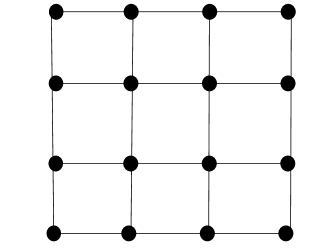
(a) Square lattice.

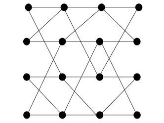
(b) Sparse-randomly connected lattice.

Figure 1: Schematics of lattices.

2.2 Model with energy conservation

Before presenting our model, we first describe a model for a thermally isolated system. We describe the stochastic time evolution in which the stationary distribution is given by the microcanonical ensemble associated with the Hamiltonian $H(\sigma,p)$. The stochastic process satisfies the detailed balance condition with respect to the uniform distribution on the energy surface $H(\sigma,p)=E$, where $E$ is the total energy, which is invariant under time evolution.

We perform the following five procedures at one step:

1. A site $i\in\Lambda$ is chosen randomly with equal probability.

2. The potential energy difference $dE$ is calculated for a transition $\sigma_{i}\to\sigma_{i}^{\prime}$ chosen randomly with equal probability.

3. The transition $\sigma_{i}\to\sigma_{i}^{\prime}$ is accepted if $p_{i}-dE\geq 0$, and then the kinetic energy is changed to $p_{i}^{\prime}=p_{i}-dE$.

4. A site $k$ and another site $j\in B_{k}$ are chosen randomly.

5. The transition $(p_{k},p_{j})\to(p_{k}-dp,p_{j}+dp)$ is accepted if $p_{k}-dp\geq 0$, where $dp$ is a numerical parameter.

Let $(p_{i}^{0})_{i\in\Lambda}$ be a collection of the initial value of kinetic energy for each site. From the evolution rule, $p_{i}$ is written as $p_{i}=p_{i}^{0}+n_{i}+m_{i}dp$, where $n_{i},m_{i}\in\mathbb{Z}$. The set of all possible values of $p_{i}$ is denoted by $\mathbb{P}_{i}$. The phase space of the model $\Sigma$ as a function of $E$ is then expressed by the discrete set

$$\Sigma(E)=\{(\sigma,p)|H(\sigma,p)=E,\ \sigma_{i}\in\{1,\cdots,q\},\ p_{i}\in\mathbb{P}_{i},\ i\in\Lambda\}.$$ (4)

The transition probability determined by the procedures is expressed as $W(\sigma^{\prime},p^{\prime}|\sigma,p)$. Let $t\in\mathbb{Z}$ be the discrete time and $P_{t}(\sigma,p)$ be the probability of taking the state $(\sigma,p)$ at $t$-step. Then, we have

$$P_{t+1}(\sigma,p)=\sum_{\sigma^{\prime},p^{\prime}}W(\sigma,p|\sigma^{\prime},p^{\prime})P_{t}(\sigma^{\prime},p^{\prime}).$$ (5)

Because $W(\sigma^{\prime},p^{\prime}|\sigma,p)=W(\sigma,p|\sigma^{\prime},p^{\prime})$ holds, the stationary distribution is given by the microcanonical form

$$P_{\rm mc}(\sigma,p)=\frac{1}{|\Sigma(E)|}\delta(H(\sigma,p),E),$$ (6)

where $|\Sigma(E)|$ denotes the number of elements of set $\Sigma(E)$.

2.3 Model with two heat baths

In the model, we attach two heat baths, one on the left side $i_{x}=1$ and one on the right side $i_{x}=L_{x}$ of the system introduced in the previous subsection. The temperatures of the left and right heat baths are denoted by $T_{L}$ and $T_{R}$, respectively. The stochastic time evolution of the model is given by imposing an additional rule at the boundaries. We perform the following procedures when a site $i$ with $i_{x}=1$ or $i_{x}=L_{x}$ is chosen in procedure 1 of the time evolution described in the previous subsection:

1. The potential energy difference $dE$ is calculated for a transition $\sigma_{i}\to\sigma_{i}^{\prime}$ chosen randomly.

2. The transition $\sigma_{i}\to\sigma_{i}^{\prime}$ is accepted with the probability $w(\sigma_{i}\to\sigma_{i}^{\prime})$, where

   $$w(\sigma_{i}\to\sigma_{i}^{\prime})=\frac{1}{2}\left(1-\tanh\left(\frac{dE}{2T}\right)\right)$$ (7)

   with $T=T_{L}$ for $i_{x}=1$ and $T=T_{R}$ for $i_{x}=L_{x}$.

3. The value of $p_{i}$ is replaced with a new one sampled from the distribution

   $$P(p_{i})=\frac{1}{T}e^{-\frac{p_{i}}{T}}$$ (8)

   with $T=T_{L}$ for $i_{x}=1$ and $T=T_{R}$ for $i_{x}=L_{x}$. We here note that $p_{i}$ takes positive value.

Note that (7) satisfies the detailed balance condition

$$\frac{w(\sigma\to\sigma^{\prime})}{w(\sigma^{\prime}\to\sigma)}=e^{-\frac{dE}{T}}.$$ (9)

The stochastic rule in the previous subsection is used except at the boundaries $i_{x}=1$ and $i_{x}=L_{x}$. The transition probability determined by the procedures is expressed as $\tilde{W}(\sigma^{\prime},p^{\prime}|\sigma,p)$. Let $t\in\mathbb{Z}$ be the discrete time and $\tilde{P}_{t}(\sigma,p)$ be the probability of taking state $(\sigma,p)$ at each $t$-step. Then, we have

$$\tilde{P}_{t+1}(\sigma^{\prime},p^{\prime})=\sum_{\sigma,p}\tilde{W}(\sigma^{\prime},p^{\prime}|\sigma,p)\tilde{P}_{t}(\sigma,p).$$ (10)

When $T_{L}=T_{R}=T$, the detailed balance condition

$$\frac{\tilde{W}(\sigma^{\prime},p^{\prime}|\sigma,p)}{\tilde{W}(\sigma,p|\sigma^{\prime},p^{\prime})}=e^{-\frac{dE}{T}}$$ (11)

holds. Thus, the stationary distribution is given by the canonical form

$$P_{\rm can}(\sigma,p)=\frac{1}{Z_{\rm tot}(\beta)}e^{-\beta H(\sigma,p)},$$ (12)

where $Z_{\rm tot}(\beta)=\sum_{\sigma,p}e^{-\beta H(\sigma,p)}$.

3 Equilibrium statistical mechanics

In this section, for reference in studying dynamical processes, we confirm some results of equilibrium statistical mechanics using the canonical ensemble

$$P_{\rm can}(\sigma)=\frac{1}{Z(\beta)}e^{-\frac{\beta}{2}\sum_{i\in\Lambda}\sum_{j\in B_{i}}\delta(\sigma_{i},\sigma_{j})}$$ (13)

for the configuration space of $\sigma$, where $P_{\rm can}(\sigma)=\sum_{p}P_{\rm can}(\sigma,p)$. We study

$$m=\lim_{|\Lambda|\to\infty}\sum_{\sigma}P_{\rm can}(\sigma)\frac{\sum_{i}\delta(\sigma_{i},1)}{|\Lambda|}$$ (14)

with an infinitely small external potential $-\sum_{i}h_{\rm ex}\delta(\sigma_{i},1)$ in the Hamiltonian, and the free energy density defined as

$$f=-\lim_{|\Lambda|\to\infty}\frac{T}{|\Lambda|}\log Z.$$ (15)

It should be noted that the free energy density $f$ and the partition function $Z$ are defined in the configuration space of $\sigma$.

In the calculation of $m$ and $f$, we conjecture that the contribution from loops in the lattice can be ignored in the large-size limit ORT ; Mezard ; Dembo . On the basis of this conjecture, the thermodynamic phase can be determined using the model on a Cayley tree with three branches corresponding to coordination number 4. Concretely, it has been known that $m$ and $f$ are calculated from the probability of the state $\sigma\in\{1,\cdots,q\}$ at a site connected with a cavity site, which is denoted as $u(\sigma)$. As shown in Appendix A, we first have the self-consistent equation for $u(\sigma)$,

$$u(\sigma)=\frac{\left[\gamma u(\sigma)+1\right]^{3}}{\sum_{\sigma}\left[\gamma u(\sigma)+1\right]^{3}},$$ (16)

with $\gamma=e^{\beta}-1$. Using the solutions of (16), we express the order parameter $m(\beta)$ and the free energy density $f(\beta)$ as

$$m(\beta) =\frac{[\gamma u(1)+1]^{4}}{\sum_{\sigma}[\gamma u(\sigma)+1]^{4}},$$ (17)

$$f(\beta) =-\beta^{-1}\log\frac{\sum_{\sigma}[\gamma u(\sigma)+1]^{4}}{\left[\gamma\sum_{\sigma}u^{2}(\sigma)+1\right]^{2}}.$$ (18)

Here we notice that (16) has the trivial solution $u_{0}(\sigma)\equiv 1/q$ for any $\beta$. There exists a temperature $\beta_{\rm sp}$ beyond which (16) has another solution denoted as $u_{*}(\sigma)$, where

$$u_{*}(\sigma)=\begin{cases}c_{*}(\beta)&(\sigma=1)\\ \frac{1-c_{*}(\beta)}{q-1}&(2\leq\sigma\leq q)\end{cases}$$ (19)

with $c_{*}\not=1/q$. The temperature $\beta_{\rm sp}$ is called the spinodal point. Using these two solutions $u_{0}$ and $u_{*}$, we have $(m_{0}(\beta),m_{*}(\beta))$ and $(f_{0}(\beta),f_{*}(\beta))$. We display $(m_{0}(\beta),m_{*}(\beta))$ in Fig. 2, and $(f_{0}(\beta),f_{*}(\beta))$ in Fig. 2 for the case $q=10$. The equilibrium transition temperature $\beta_{c}$ is identified as $f_{0}(\beta_{c})=f_{*}(\beta_{c})$.

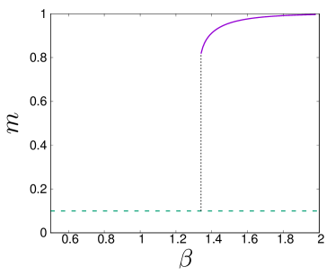
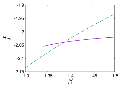
Figure 2: (a) $m$ as a function of $\beta$ for the case $q=10$. The solid (purple) and dashed (green) line represent $m_{*}(\beta)$ and $m_{0}(\beta)$, respectively. The vertical line indicates $\beta=\beta_{\rm sp}$. (b) $f$ as a function of $\beta$ for the case $q=10$. The solid (purple) and dashed (green) line represent $f_{*}(\beta)$ and $f_{0}(\beta)$, respectively.

To study the free energy landscape, we define

$$\tilde{f}(\beta,c)=-\beta^{-1}\log\frac{\sum_{\sigma}[\gamma\tilde{u}(\sigma)+1]^{4}}{\left[\gamma\sum_{\sigma}\tilde{u}^{2}(\sigma)+1\right]^{2}},$$ (20)

where

$$\tilde{u}(\sigma)=\begin{cases}c&(\sigma=1)\\ \frac{1-c}{q-1}&(2\leq\sigma\leq q).\end{cases}$$ (21)

Setting $c_{0}=1/q$, we have $f_{0}(\beta)=\tilde{f}(\beta,c_{0})$ and $f_{*}(\beta)=\tilde{f}(\beta,c_{*})$. Furthermore, by straightforward calculation, we confirm

$$\frac{\partial}{\partial c}\left(e^{-\beta\tilde{f}(\beta,c)}\right)=0$$ (22)

at $c=c_{0}$ and $c=c_{*}$. See Appendix A.4 for the derivation. Therefore, displaying $\tilde{f}(\beta,c)$ in Fig. 3, we see that the solution $u_{*}$ appears at the spinodal point $\beta=\beta_{\rm sp}$, and the equilibrium transition occurs at $\beta=\beta_{c}$. We also find that $\partial^{2}\tilde{f}/\partial c^{2}=0$ at $c=c_{0}$ and $\beta=\beta_{\rm un}$, which means that the trivial solution $u_{0}$ loses stability. Letting $F(u)$ be the right-hand side of (16), the solutions of the self-consistent equation are given by the fixed points $u_{n+1}=F(u_{n})$. The temperature $\beta_{\rm un}$ is also characterized by the onset of the instability of the trivial solution for this iteration equation. For the case $q=10$, we find that $\beta_{\rm sp}\simeq 1.34$, $\beta_{c}\simeq 1.39$, and $\beta_{\rm un}\simeq 1.78$.

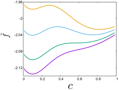
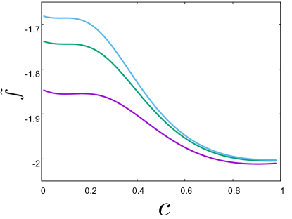
Figure 3: Free energy landscapes for (a) $\beta<\beta_{\rm sp},\ \beta=\beta_{\rm sp},\ \beta=\beta_{c},\$and $\beta_{c}<\beta<\beta_{\rm un}$ from below, and (b) $\beta_{c}<\beta<\beta_{\rm un},\ \beta=\beta_{\rm un},$ and $\ \beta>\beta_{\rm un}$ from below.

4 Numerical simulation

Throughout this section, we simulate the model with $q=10$ and choose the numerical parameter $dp=0.01T_{c}$. Before presenting our results, in Fig. 4, we show the statistical average of $\sum_{i}\delta(\sigma_{i},1)/|\Lambda|$ for the model given in Sec. 2, where $T_{L}=T_{R}=\beta^{-1}$ and $L_{x}=L_{y}=100$. The numerical result agrees with the theoretical calculation in Sec. 3.

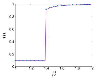
Figure 4: Circle (green) symbols represent the simulation result for the model given in Sec. 2, with $T_{L}=T_{R}=\beta^{-1}$. The solid (purple) curve is the theoretical result obtained in Sec. 3.

Then, we prepare a metastable ordered phase of the temperature $T_{L}$ in $1\leq i_{x}\leq L_{x}/2$ and a stable disordered phase of the temperature $T_{R}$ in $L_{x}/2+1\leq i_{x}\leq L_{x}$. Here, we fix $T_{L}=1.01T_{c}$ so that the ordered phase is metastable, and $T_{R}$ is assumed to be greater than $T_{c}$ so that the disordered phase is stable. We prepare configurations at $t=0$ via the following steps. First, we remove the coupling between $i_{x}=L_{x}/2$ and $i_{x}=L_{x}/2+1$ by setting $B_{i}^{+}=\emptyset$ for $i_{x}=L_{x}/2$. Second, we prepare a configuration where $\sigma_{i}=1$ and $p_{i}=T_{L}$ for any $i$ satisfying $i_{x}\leq L_{x}/2$, while each $\sigma_{i}$ is randomly chosen with equal probability and $p_{i}=T_{R}$ for any $i$ satisfying $i_{x}>L_{x}/2+1$. Third, we make the system evolve up to 50 MCS. The reached configuration is set to be an initial state at $t=0$ in the following analysis. Note that $s$ MCS corresponds to the $t=sL_{x}L_{y}$ step in the procedure described in Sec. 2.

The stable disordered phase grows from the initial configuration. To describe the phase growth, we observe an order parameter profile defined as

$$\phi(x,t)\equiv\frac{q{m(x,t)-1}}{q-1}$$ (23)

with

$$m(x,t)\equiv\frac{1}{L_{y}}\sum_{y=1}^{L_{y}}\delta(\sigma_{x,y},1)$$ (24)

for $1\leq x\leq L_{x}$. We define the value $\phi(x,t)$ for any real $x$ via linear interpolation. Similarly, we define the temperature field as

$$T(x,t)\equiv\frac{1}{L_{y}}\sum_{y=1}^{L_{y}}p_{x,y}.$$ (25)

Examples of $\phi(x,t)$ and $T(x,t)$ are displayed in Fig. 5 and  5.

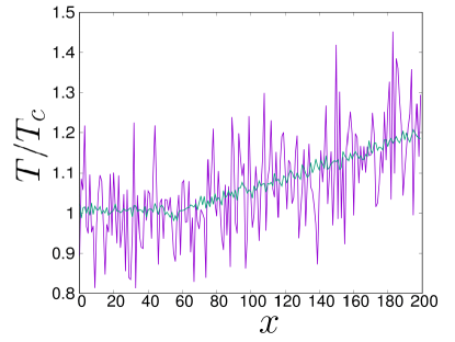
Figure 5: (a) $\phi(x,t)$ as a function of $x$ at $t=5\times 10^{6}$ MCS for the system with $L_{x}=200,L_{y}=100,T_{R}=1.2T_{c}$, and $T_{L}=1.01T_{c}$. The purple and green graphs represent one snap shot and the average over 100 samples, respectively. (b) $T(x,t)/T_{c}$ as a function of $x$ for the same condition as (a). The colors of lines correspond to the graphs in (a).

We identify the interface position $X(t)$ from $\phi(x,t)$ such that $\phi(X(t),t)=0.5$. $X(t)$ is uniquely determined because $\phi$ crosses 0.5 only once as far as we observe. $R(t)$ denotes the displacement of the interface $|X(t)-X(0)|$. In Fig. 6, we show an example of configuration $\sigma$ with the interface position.

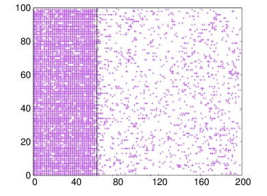
Figure 6: Configuration of $\sigma$ at $t=5\times 10^{6}$ MSC for the system with $L_{x}=200,L_{y}=100$. The dots represent sites where $\sigma_{i}=1$. The solid line represents the interface position.

In Fig. 7, we show the statistical average of $R(t)$ for the case $T_{R}=3T_{c}>T_{\rm sp}$. The five graphs correspond to results for different systems sizes $(L_{x},L_{y})=(100,100)$, $(200,100)$, $(300,100)$, $(100,200)$, and $(200,200)$. Because the interface eventually reaches the left boundary and does not move anymore, all the curves become flat in the long-time limit. The guideline represents $R(t)=At^{0.5}$ with $A=0.18$. We also confirmed that the $L_{y}$ dependence is hardly visible for this system size. From these results, we reasonably conjecture that the behavior in the large-$L_{x}$ limit is described by the phase-field model because the extent of the metastability $\Delta$ is evaluated as $0.05$, as shown in Appendix B.

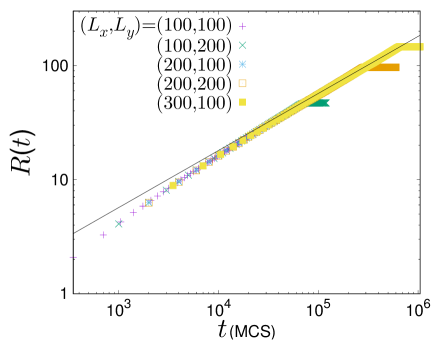
Figure 7: $R(t)$ versus $t$ for $T_{R}=3T_{c}$. The average of 100 samples was taken for the system with different system sizes. The solid line represents $R(t)=At^{0.5}$ with $A=0.18$.

An unexpected behavior of $R(t)$ is observed for the case $T_{R}=1.2T_{c}>T_{\rm sp}$. As shown in Fig. 8, four graphs for different system sizes, $(L_{x},L_{y})=(100,100),(200,100),(300,100)$, and $(400,100)$ do not overlap, while the $L_{y}$ dependence is hardly visible. We then consider a finite size scaling to plot $R/L_{x}$ as a function of $Dt/L_{x}^{2}$, where the thermal diffusion constant $D$ is estimated as $1.9\times 10^{-2}$ from the measurement of the relaxation time of the temperature field, as shown in Appendix C. The result is displayed in Fig. 8. We find the scaling relation

$$\frac{R(t)}{L_{x}}=\bar{\mathcal{R}}\left(\frac{Dt}{L^{2}_{x}}\right)$$ (26)

works well, where $\bar{\mathcal{R}}$ is a scaling function. The scaling function indicates the cross-over from $\bar{\mathcal{R}}(z)\simeq z^{0.5}$ to $\bar{\mathcal{R}}(z)\simeq z^{\alpha}$ with $0.5\leq\alpha\leq 1$. It should be noted that the scaling relation in the late stage is not observed in the phase-field model.

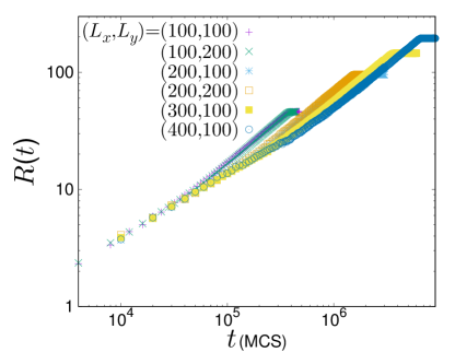
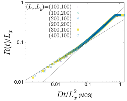
Figure 8: (a). $R(t)$ versus $t$ for $T_{R}=1.2T_{c}$. The average of 100 samples was taken for the system with different system sizes. (b) $R(t)/L_{x}$ as a function of $z=Dt/L_{x}^{2}$. The two guidelines are $Az^{0.5}$ and $A^{\prime}z^{0.75}$, where $A=0.32$ and $A^{\prime}=0.60$, respectively.

The exponent $\alpha$ depends on the value of $T_{R}$. Decreasing $T_{R}$ further, we find that the late stage becomes dominant and $\alpha$ increases. For the case $T_{R}=T_{L}=1.01T_{c}<T_{\rm sp}$, $\alpha$ turns out to be close to unity, as shown in Fig. 9.

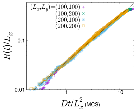
Figure 9: $R/L_{x}$ as a function of $Dt/L_{x}^{2}$ for the case $T_{R}=1.01T_{c}$. The guideline represents $Az^{0.95}$ with $A=3.6\times 10^{-2}$.

To our best knowledge, the cross-over behavior has never been reported in previous studies. This observation raises a question about if this behavior is a unique feature of the stochastic model. In order to answer this question, we carefully study finite-size effects for the deterministic phase-field model. Specifically, we perform numerical simulations of the model used in Karma-noise . Concretely, we study the following equations of the order parameter field $\phi(x,t)$ and the dimensionless temperature field $\theta(x,t)$:

$$\frac{\partial\phi}{\partial t} =\partial_{x}^{2}\phi+\phi-\phi^{3}-\theta(1-\phi^{2})^{2},$$ (27)

$$\frac{\partial\theta}{\partial t} =D\partial_{x}^{2}\theta+\frac{1}{2}\frac{\partial p(\phi)}{\partial t},$$ (28)

where $\theta(x,t)$ is related to $T(x,t)$ as

$$\theta(x,t)=\frac{c_{p}}{T_{c}(\delta s)}{\left(T(x,t)-T_{c}\right)}.$$ (29)

The functional form of $p(\phi)$ is given by

$$p(\phi)=\frac{15}{8}\left(\phi-\frac{2\phi^{3}}{3}+\frac{\phi^{5}}{5}\right).$$ (30)

We fix $T_{L}=1.01T_{c}$ and $D=1$. The results are shown in Figs. 10, 10 and 10. We observe the same behavior as that observed in the statistical mechanics model. We thus conclude that the cross-over behavior is not specific to stochastic systems.

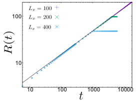
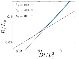
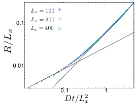
Figure 10: Interface displacement for the phase-field model. (a) $R(t)$ as a function of $t$ for $T_{R}=4.0T_{c}$. The guideline represents $At^{0.5}$ with $A=1.53$. (b) $R/L_{x}$ as a function of $Dt/L_{x}^{2}$ for $T_{R}=1.05T_{c}$. The guidelines represent $Az^{0.5}$ and $A^{\prime}z^{0.9}$ with $A=7.6\times 10^{-2}$ and $A^{\prime}=0.16$. (c) $R/L_{x}$ as a function of $Dt/L_{x}^{2}$ for $T_{R}=1.01T_{c}$. The guidelines represent $Az^{0.5}$ and $A^{\prime}z$ with $A=2.6\times 10^{-2}$ and $A^{\prime}=5.6\times 10^{-2}$.

Furthermore, for the phase-field model, we study $T_{R}$-dependence more systematically. Let $t_{c}$ be the cross-over time. In Fig. 11, we plot $R(t_{c})/L_{x}$ as a function of $(T_{R}-T_{c})/T_{c}$. $R(t)$ is defined in the same way as done for the stochastic model. We then observe

$$\frac{R(t_{c})}{L_{x}}\simeq A\left(\frac{T_{R}-T_{c}}{T_{c}}\right)^{0.75}$$ (31)

with $A=0.30$. Since the interface position moves up to $L_{x}/2$, the interface reaches the boundary before the cross-over occurs for temperatures $T_{R}$ satisfying ${R(t_{c})}\geq L_{x}/{2}$. In this case, only $R(t)\sim t^{0.5}$ is observed. On the other hand, as the temperature $T_{R}$ is close to $T_{c}$ with large $L_{x}$ fixed, $R(t_{c})/L_{x}$ tends to zero. This means that only $R(t)\sim t^{\alpha}$ with $\alpha\simeq 1$ is observed. Note that if we take the limit $L_{x}\to\infty$ first, $R(t)\sim t^{0.5}$ is observed. However, when we observe the interface motion in finite-size systems, the behavior depends on the order of the three limits $L_{x}\to\infty$, $t\to\infty$, and $T_{R}\to T_{c}$.

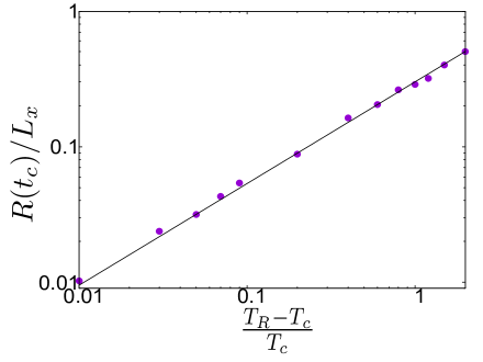
Figure 11: $T_{R}$-dependence of $R(t_{c})/L_{x}$. The guideline is given by (31).

5 Concluding remarks

We have proposed a $q$-state Potts model with an additional variable representing the kinetic energy at each site. By designing a two-dimensional lattice, where each site is sparse-randomly connected in one direction and local in the other direction, we have explicitly calculated the thermodynamic properties via equilibrium statistical mechanics. Simulating this model, we have numerically observed that the interface between the stable and metastable phases moves following the scaling relation (26) with the scaling function $\bar{\mathcal{R}}(z)$. The scaling function shows a cross-over from $\bar{\mathcal{R}}(z)\simeq z^{0.5}$ to $\bar{\mathcal{R}}(z)\simeq z^{\alpha}$, where the cross-over value of $z$ and the exponent $\alpha$ depends on the temperature of the heat bath attached to the stable phase. We have only analyzed the case $q=10$. Changing the value of $q$ influences the quantitative behavior through the $\Delta$-dependence. We conjecture that the $\Delta$ dependence in the large system size limit should be consistent with the theoretical result for the phase-field model HS , because our stochastic model belongs to the same universality class as the phase-field model. In ending this paper, we make two remarks.

The first is on the status of our model. We note that our model is rarely realizable in experiments, like a more familiar mean-field type model, where a site $(i_{x},i_{y})$ is connected to all sites in the $i_{x}+1$ layer. Despite apparent unphysical nature of the random lattice, the phase growth in our model is qualitatively same as that for the model on the square lattice, as shown in Figs. 12, 12, and 12. This is a special property of our model, because the mean-field type model shows a different behavior HOS2 . Thus, toward the microscopic derivation of a coupled equation for the order parameter field and the temperature field, numerical results for our model should be theoretically explained by extending the analysis shown in Sec. 3 and Appendix A.

The second remark is on the Mullins-Sekerka instability MS . The instability of propagating interfaces was studied in the phase-field model for the case $\Delta\geq 1$ Kupf ; Braun . We do not clearly understand the instability condition for the case $\Delta<1$. Nevertheless, in any cases, it is clear that the instability is not observed in our model on the sparse-randomly connected lattice, because there is no spatial correlation in the vertical direction. While this aspect may be a disadvantage of the model, we note that the instability is not our main concern. For the model on the square lattice, there remains a possibility that Mullins-Sekerka instability could appear for larger system sizes than we studied. Clarifying the instability condition is left for future study.

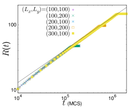
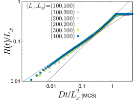
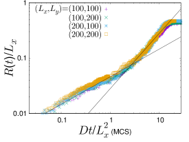
Figure 12: Interface displacement of the $q$-state Potts model on the square lattice. The value of $D$ is measured as $0.02$ in the same way as shown in Appendix C. The value of $T_{c}$ for $q=10$ was calculated exactly Wu . (a) $R(t)$ as a function of $t$ for $T_{R}=3.0T_{c}$. The guideline represents $At^{0.5}$ with $A=0.13$. (b) $R/L_{x}$ as a function of $Dt/L_{x}^{2}$ for $T_{R}=1.2T_{c}$. The guidelines represent $Az^{0.5}$ and $A^{\prime}z^{0.75}$ with $A=0.28$ and $A^{\prime}=0.38$. (c)$R/L_{x}$ as a function of $Dt/L_{x}^{2}$ for $T_{R}=1.01T_{c}$. The guidelines represent $Az^{0.5}$ and $A^{\prime}z$ with $A=4.6\times 10^{-2}$ and $A^{\prime}=2.8\times 10^{-2}$.

Data Availibility  The datasets generated during and/or analysed during the current study are available from the corresponding author on reasonable request.

Conflict of Interest    The authors have no financial or proprietary interests in any material discussed in this article.

Appendix A Derivation of the formulas in Sec. 3

In this section, we derive formulas (16), (17), (18), and (22) in Sec. 3.

A.1 Derivation of (16)

We study a Cayley tree with a root site connected with four sites in the first generation. Each site in the $n$-th generation $(n\geq 1)$ is connected with three sites in the $n+1$-th generation. See Fig. 13 for the illustration of the Cayley tree.

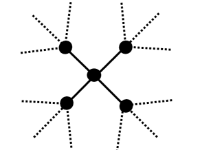
Figure 13: Illustration of the Cayley tree.

Let $Z$ be the partition function of the Potts model on the lattice. We consider the partition function of a system in which a root site is replaced by the cavity and the state of a site in the first generation is fixed as $\sigma^{\prime}\in\{1,\cdots,q\}$, which is denoted by $\tilde{Z}_{1}(\sigma^{\prime})$. $Z$ is then the partition function of the model expressed as

$$Z=\sum_{\sigma}\left(\sum_{\sigma^{\prime}}e^{\beta\delta(\sigma,\sigma^{\prime})}\tilde{Z}_{1}(\sigma^{\prime})\right)^{4}.$$ (A.1)

A graphical representation is displayed in Fig. 14.

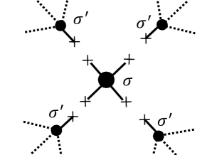
Figure 14: Graphical representation of (A.1).

By setting

$$\gamma \equiv e^{\beta}-1,$$ (A.2)

$$G_{1} \equiv\sum_{\sigma}\tilde{Z_{1}}(\sigma),$$ (A.3)

we rewrite (A.1) as

$$Z=\sum_{\sigma}\left(\gamma\tilde{Z}_{1}(\sigma)+G_{1}\right)^{4}.$$ (A.4)

Defining $\tilde{Z}_{n}(\sigma)$ and $G_{n}$ similarly, we have the iterative equation

$$\tilde{Z}_{n}(\sigma)=\left(\gamma\tilde{Z}_{n+1}(\sigma)+G_{n}\right)^{3},$$ (A.5)

whose graphical representation is shown in Fig. 15.

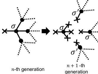
Figure 15: Graphical representation of (A.5).

We define $u_{n}(\sigma)$ as

$$u_{n}(\sigma)\equiv\frac{\tilde{Z_{n}}(\sigma)}{G_{n}},$$ (A.6)

which corresponds to the probability of the state $\sigma$ of the cavity-connected site in the $n$-th generation. By substituting (A.6) into (A.5), we obtain

$$G_{n}u_{n}(\sigma) =G_{n+1}^{3}\left[\gamma u_{n+1}(\sigma)+1\right]^{3}.$$ (A.7)

We also have

$$G_{n}=G_{n+1}^{3}\sum_{\sigma}\left[\gamma u_{n+1}(\sigma)+1\right]^{3}$$ (A.8)

using $\sum_{\sigma}u_{n}(\sigma)=1$. From (A.7) and (A.8), we derive the iterative equation for $u_{n}(\sigma)$,

$$u_{n}(\sigma)=\frac{\left[\gamma u_{n+1}(\sigma)+1\right]^{3}}{\sum_{\sigma}\left[\gamma u_{n+1}(\sigma)+1\right]^{3}}.$$ (A.9)

Assuming homogeneity in the equilibrium state, $u_{n}(\sigma)$ is independent of $n$ in the large-size limit. This provides (16).

A.2 Derivation of (17)

The order parameter $m$ for the model is calculated by the expectation value of $\delta(\sigma,1)$ at the root site. That is,

$$m=\frac{1}{Z}\sum_{\sigma}\delta(\sigma,1)\left[\gamma\tilde{Z}_{1}(\sigma)+G_{1}\right]^{4}.$$ (A.10)

Using the expression given in (A.4), we have

$$m=\frac{[\gamma u_{1}(1)+1]^{4}}{\sum_{\sigma}[\gamma u_{1}(\sigma)+1]^{4}}.$$ (A.11)

By replacing $u_{1}$ with the solution of the self-consistent equation (16), we obtain (17).

A.3 Derivation of (18)

To derive the free energy density, we use a tactical method manipulating graphs. We first remove one edge connected to the root site. The partition function of this system with $\sigma$ at the root site and $\sigma^{\prime}$ at the other site connected by the removed edge is $\tilde{Z}_{0}(\sigma)\tilde{Z}_{1}(\sigma^{\prime})$. See Fig. 16. We thus express the partition function $Z$ as

$$Z =\sum_{\sigma,\sigma^{\prime}}e^{\beta\delta(\sigma,\sigma^{\prime})}\tilde{Z_{0}}(\sigma)\tilde{Z_{1}}(\sigma^{\prime})$$ (A.12)

$$=G_{0}G_{1}\left[\gamma\sum_{\sigma}u_{0}(\sigma)u_{1}(\sigma)+1\right],$$ (A.13)

where $G_{0}\equiv\sum_{\sigma}\tilde{Z}_{0}(\sigma)$ and $u_{0}(\sigma)\equiv\tilde{Z}_{0}(\sigma)/G_{0}$. Note that $u_{0}(\sigma)$ also satisfies (A.9).

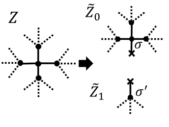
Figure 16: By removing one edge, we get two rooted graphs. $\times$ represents the cavity.

Next, we prepare four independent systems. The partition function of the total system is $Z^{4}$. We remove one edge connected to the root site for each graph. Then, we combine four graphs with the root site by adding one site. See Fig. 17. The partition function of this system, $\check{Z_{0}}$, is expressed as

$$\check{Z_{0}}=G_{0}^{4}\sum_{\sigma}\left[\gamma u_{0}(\sigma)+1\right]^{4}.$$ (A.14)

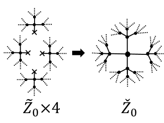
Figure 17: By adding one site, we combine four graphs with the root site.

Similarly, another Cayley tree is obtained by combining the other graphs with another added site, and the partition function is written as

$$\check{Z_{1}}=G_{1}^{4}\sum_{\sigma}\left[\gamma u_{1}(\sigma)+1\right]^{4}.$$ (A.15)

The free energies of the original system and the new system are $-T\log Z^{4}$ and $-T\log\check{Z_{0}}\check{Z_{1}}$, respectively. The difference in free energy is equal to $2f$, where $f$ is the free energy density, because the two systems have the same free energy density in the large-size limit and the new system is the original system with two sites added. That is,

$$-T\log\check{Z_{0}}\check{Z_{1}}+T\log Z^{4}=2f.$$ (A.16)

This is rewritten as

$$e^{-\beta f}=\left(\frac{\check{Z}_{0}\check{Z}_{1}}{Z^{4}}\right)^{1/2}$$ (A.17)

$$=\left(\frac{\sum_{\sigma^{\prime}}[\gamma u_{0}(\sigma^{\prime})+1]^{4}\sum_{\sigma^{\prime\prime}}[\gamma u_{1}(\sigma^{\prime\prime})+1]^{4}}{\left[\gamma\sum_{\sigma}u_{0}(\sigma)u_{1}(\sigma)+1\right]^{4}}\right)^{1/2}.$$ (A.18)

By replacing $u_{0}$ and $u_{1}$ with the solution of the self-consistent equation (16), we obtain (18).

A.4 Derivation of (22)

For later convenience, we set

$$\tilde{c}\equiv\frac{1-c}{q-1}.$$ (A.19)

From the definition of $\tilde{f}$ given in (20), the left-hand side of (22) is calculated as

$$\frac{\partial}{\partial c}e^{-\beta\tilde{f}(\beta,c)}$$

$$=4\gamma\frac{(\gamma c+1)^{3}-(\gamma\tilde{c}+1)^{3}}{(\gamma c^{2}+\gamma(q-1)\tilde{c}^{2}+1)^{2}}$$

$$-4\gamma(c-\tilde{c})\frac{(\gamma c+1)^{4}+(q-1)(\gamma\tilde{c}+1)^{4}}{(\gamma c^{2}+\gamma(q-1)\tilde{c}^{2}+1)^{3}}.$$ (A.20)

The self-consistent equation (16) is expressed as

$$(\gamma\tilde{c}+1)^{3}=\frac{\tilde{c}}{c}(\gamma c+1)^{3}.$$ (A.21)

Thus, the right-hand side of (A.20) for the special values of $c$ satisfying (A.21) is calculated as

$$4\gamma\frac{(\gamma c+1)^{3}(c-\tilde{c})}{c(\gamma c^{2}+\gamma(q-1)\tilde{c}+1)^{2}}$$

$$\times\left(1-\frac{\gamma c^{2}+\gamma(q-1)\tilde{c}^{2}+c+(q-1)\tilde{c}}{\gamma c^{2}+\gamma(q-1)\tilde{c}^{2}+1}\right),$$ (A.22)

which turns out to be zero from (A.19).

Appendix B Estimation of $\Delta$

In this section, we estimate the value of $\Delta$ defined by (1) for the model we study.

We first calculate the energy density $h$ defined as

$$h\equiv\lim_{|\Lambda|\to\infty}\frac{1}{|\Lambda|}\sum_{\sigma,p}P_{\rm can}(\sigma,p)H(\sigma,p),$$ (B.23)

where $P_{\rm can}(\sigma,p)$ is given in (12). Using the free energy density $f$ calculated in Sec. 3, we express the energy density $h$ as

$$h=T+g,$$ (B.24)

where $g$ is the potential energy density given by

$$g(\beta)\equiv\frac{\partial}{\partial\beta}\left(\beta f(\beta)\right).$$ (B.25)

As with the free energy density, $g_{0}(\beta)$ and $g_{*}(\beta)$ denote the potential energy densities corresponding to the trivial solution $u_{0}$ and the nontrivial solution $u_{*}$ of (16), respectively. In Fig. 18, $g_{0}(\beta)$ and $g_{*}(\beta)$ are displayed. Then, the latent heat per unit volume $T_{c}\delta s$ at the equilibrium transition temperature is determined by the entropy jump defined as

$$\delta s\equiv\beta_{c}(g_{0}(\beta_{c})-g_{*}(\beta_{c})).$$ (B.26)

For the model with $q=10$, we obtain $T_{c}\delta s\simeq 1.07$. Next, we consider the heat capacity per unit volume $C$ expressed as

$$C(\beta)\equiv\frac{\partial h}{\partial T}=1+\frac{\partial g}{\partial T}.$$ (B.27)

Using similar notations, we obtain $C_{0}(\beta)$ and $C_{*}(\beta)$ from $g_{0}(\beta)$ and $g_{*}(\beta)$. These are shown at the bottom of Fig. 18. For the cases $q=10$ and $T_{L}=1.01T_{c}$, we obtain $C_{*}(T_{L})\simeq 6.95$. Therefore, for the model we numerically study, we have

$$\Delta\simeq 0.05,$$ (B.28)

which is less than unity. Note that in the stochastic model studied in this paper, $C$ corresponds to $c_{p}$ in the phase-field model.

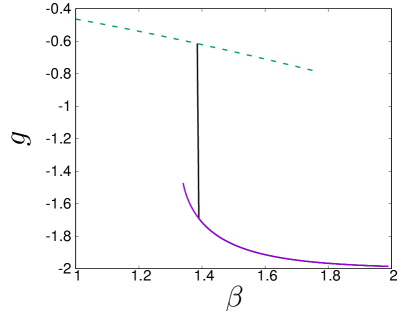
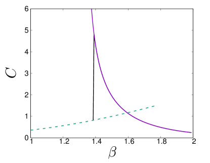
Figure 18: (a) Potential energy density $g$ as a function of $\beta$. The solid (purple) line represents $g=g_{*}$ in the range $\beta>\beta_{\rm sp}$. The dashed (green) line represents $g=g_{0}$ in the range $\beta<\beta_{\rm un}$. The black line indicates $\beta=\beta_{c}$. (b) Heat capacity per unit volume $C$ as a function of $\beta$. The styles (colors) of lines correspond to the graphs in (a).

Appendix C Estimation of $D$

In this section, we estimate the value of the thermal diffusion constant $D$ by measuring the relaxation property of the temperature profile $T(x,t)$, where

$$T(x,t)\equiv\frac{1}{L_{y}}\sum_{y=1}^{L_{y}}p_{x,y}(t).$$ (C.29)

For simplicity, we study the case $T_{R}=T_{L}=1.2T_{c}$ with the initial condition

$$T(x,0)\equiv 1.2T_{c}+\sin\left(\frac{\pi(x-1)}{L_{x}-1}\right).$$ (C.30)

To realize the initial condition $T(x,0)$, $\sigma_{i}$ is randomly chosen with equal probability and $p_{i}=T(i_{x},0)$ for any $i$. We then define the spatial average of the local temperature as

$$\bar{T}(t)\equiv\left\langle\frac{1}{L_{x}}\sum_{x=1}^{L_{x}}T(x,t)\right\rangle,$$ (C.31)

where $\langle\cdot\rangle$ denotes the average over ten independent samples. Assuming the diffusion equation for $T(x,t)$, we have

$$\frac{\bar{T}(t)}{T_{c}}=1.2+Be^{-D\pi^{2}t/L_{x}^{2}},$$ (C.32)

where $D$ is the thermal diffusion constant and $B$ is a parameter associated with the initial condition. As shown in Fig. 19, we find that the fitting of (C.31) with (C.32) works well for various system sizes with $B=1$. From this fitting, we estimate $D=1.9\times 10^{-2}$.

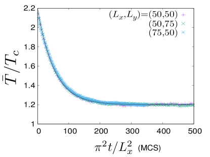
Figure 19: $\bar{T}/T_{c}$ as a function of $\pi^{2}t/L_{x}^{2}$. The solid line represents the fitting curve (C.32).

References

- (1) Callen, H. B.: Thermodynamics and an Introduction to Thermostatistics. 2nd ed. (Wiley, New York, 1985)
- (2) Pomeau, Y.: Front motion, metastability and subcritical bifurcations in hydrodynamics. Physica D 23, 3 (1986)
- (3) Stefan, J.: über die theorie der eisbildung, insbesondere über die eisbildung im polarmeere, Sitzungsberichte der Österreichischen Akademie der Wissenschaften Mathematisch- Naturwissenschaftliche Klasse. Abteilung 2, Mathematik, Astronomie, Physik, Meteorologie und Technik 965 (1889)
- (4) Stefan, J.: über die theorie der eisbildung, insbesondere über die eisbildung im polarmeere. Ann. Phys. (Leipzig) 269 (1891)
- (5) Fix, G. J.: Phase field methods for free boundary problems. In Free Boundary Problems: Theory and Applications edited by Fasano, A., Primicerio, M. (Piman, Boston, 1983), Vol. 2.
- (6) Caginalp, G.: Surface tension and supercooling in solidification theory. In Springer Lecture Notes in Physics, Applications of Field Theory to Statistical Mechanics (Springer, Berlin, 1984)
- (7) Langer, J. S.: Models of pattern formation in first-order phase transitions. In Directions in Condensed Matter Physics, edited by Grinstein, G., Mazenko, G. (World Scientific, Philadelphia, 1986)
- (8) Collins, J. B., Levine, H.: Diffuse interface model of diffusion-limited crystal growth. Phys. Rev. B 2020 (1986)
- (9) Penrose, O., Fife, P. C.: Thermodynamically consistent models of phase-field type for the kinetics of phase transition. Physica D 44 (1990)
- (10) Kobayashi, R.: Modeling and numerical simulations of dendritic crystal growth. Physica D 410 (1993)
- (11) Zener, C.: Theory of growth of spherical precipitates from solid solution. J. Appl. Phys. 20, 950 (1949)
- (12) Dewynne, J. N., Howison, S. D., Ockendon, J. R., Xie, W.: Asymptotic behavior of solutions to the Stefan problem with a kinetic condition at the free boundary. J. Austral. Math. Soc. Ser. B 81 (1989)
- (13) Löwen, H., Bechhoefer, J., Tuckerman, L. S.: Crystal growth at long times: critical behavior at the crossover from diffusion to kinetics-limited regimes. Phys. Rev. A 2399 (1992)
- (14) Hiraizumi, M., Sasa, S.-i.: Perturbative solution of a propagating interface in the phase field model. J. Stat. Mech. 103203 (2021)
- (15) Halperin, B. I., Hohenberg, P. C., Ma, S. K.: Renormalization group methods for critical dynamics. I. Recursion relations and effects of energy conservation. Phys. Rev. B 139 (1974)
- (16) Anderson, D. M., McFadden, G. B., Wheeler, A. A.: Diffuse-Interface Methods in Fluid Mechanics. Annu. Rev. Fluid Mech. 139 (1998)
- (17) Hohenberg, P. C., Halperin, B. I.: Theory of dynamic critical phenomena. Rev. Mod. Phys. 435 (1977)
- (18) Townsend, R. M., Rice, S. A.: Molecular dynamics studies of the liquid-vapor interface of water. J. Chem. Phys. 2207 (1991)
- (19) Burton, W. K., Cabrera, N., Frank, F. C.: The growth of crystals and the equilibrium structure of their surfaces. Phil. Trans. Roy. Soc. London, Ser. A 299 (1951)
- (20) Gilmer, G. H., Bennema, P.: Simulation of Crystal Growth with Surface Diffusion. J. Appl. Phys. 1347 (1972)
- (21) Müller-Krumbhaar, H.: Master-equation approach to stochastic models of crystal growth. Phys. Rev. B 1308 (1974)
- (22) Weeks, J. D., Gilmer, G. H., Jackson, K. A.: Analytical theory of crystal growth. J. Chem. Phys. 712 (1976)
- (23) Saito, Y., Müller-Krumbhaar, H.: Diffusion and relaxation kinetics in stochastic models for crystal growth. J. Chem. Phys. 1078 (1979)
- (24) Gilmer, G. H.: Computer models of crystal growth. Science 355 (1980)
- (25) Witten, T. A., Sander, L. M.: Diffusion-Limited Aggregation, a Kinetic Critical Phenomenon. Phys. Rev. B 27, 5686 (1983)
- (26) Moss, R., Harrowell, P.: Dynamic Monte Carlo simulations of freezing and melting at the 100 and 111 surfaces of the simple cubic phase in the face-centered-cubic lattice gas. J. Chem. Phys. 7630 (1994)
- (27) Novotny, M. A., et al., Simulations of metastable decay in two- and three-dimensional models with microscopic dynamics. J. Non-Cryst. Solids 356 (2000)
- (28) Wu, F. Y.: The Potts model. Rev. Mod. Phys. 235 (1982)
- (29) Kadanoff, L., Swift, J.: Transport coefficients near the liquid-gas critical point. Phys. Rev. 310 (1968)
- (30) Creutz, M.: Microcanonical monte carlo simulation. Phys. Rev. Lett. 1411 (1983)
- (31) Casartelli, M., Macellari, N., Vezzani, A.: Heat conduction in a two-dimensional Ising model. Eur. Phys. J. B 149 (2007)
- (32) Sahni, P. S., Grest, G. S., Anderson, M. P., Srolovitz, D. J.: Kinetics of the State Potts Model in Two Dimensions. Phys. Rev. Lett. 263 (1983)
- (33) Kaski, K., Nieminen, J., Gunton, J. D.: Domain growth and scaling in the Q-state Potts model. Phys. Rev. B 2998 (1985)
- (34) Clément, Sire., Satya, N., Majumdar.: Coarsening in the q-state Potts model and the Ising model with globally conserved magnetization. Phys. Rev. E 244 (1995)
- (35) Ohta, H., Rosinberg, M. L., Tarjus, G.: Morphology transition at depinning in a solvable model of interface growth in a random medium. Europhys. Lett. 16003 (2013)
- (36) Mézard, M., Montanari, A.: Information, Physics, and Computation (Oxford, England, 2009)
- (37) Dembo, A., Montanari, A.: Gibbs measures and phase transitions on sparse random graphs. Braz. J. Probab. Stat. 137 (2010)
- (38) Karma, A., Rappel, W. J.: Phase-field model of dendritic sidebranching with thermal noise. Phys. Rev. E 3614 (1999)
- (39) M. Hiraizumi, H. Ohta, and S.-i. Sasa, unpublished.
- (40) Mullins, W. W., Sekerka, R. F.: Stability of a Planar Interface During Solidification of a Dilute Binary Alloy. J. Appl. Phys. 323 (1963)
- (41) Kupfermann, R., Shochet, O., Ben-Jacob, E., Schuss, Z.: Phase-field model: boundary layer, velocity of propagation, and the stability spectrum. Phys. Rev. B 46, 16045 (1992)
- (42) Braun, R. J., McFadden, G. B., Coriell, S. R.: Morphological instability in phase-field models of solidification. Phys. Rev. E 4336 (1994)