An Error analysis of Discontinuous Finite Element Methods for the Optimal Control problems governed by Stokes equation
Abstract.
In this paper, an abstract framework for the error analysis of discontinuous finite element method is developed for the distributed and Neumann boundary control problems governed by the stationary Stokes equation with control constraints. A priori error estimates of optimal order are derived for velocity and pressure in the energy norm and the -norm, respectively. Moreover, a reliable and efficient a posteriori error estimator is derived. The results are applicable to a variety of problems just under the minimal regularity possessed by the well-posedness of the problem. In particular, we consider the abstract results with suitable stable pairs of velocity and pressure spaces like as the lowest-order Crouzeix-Raviart finite element and piecewise constant spaces, piecewise linear and constant finite element spaces. The theoretical results are illustrated by the numerical experiments.
Key words and phrases:
PDE-constrained optimization; Control-constraints; Finite element method; Discontinuous Galerkin method; Error bounds; Stokes equation1991 Mathematics Subject Classification:
65N30; 65N15; 65N12; 65K101. Introduction
We consider the following distributed control and Neumann boundary control problems governed by Stokes equations
where for distributed control problem and for Neumann boundary control problem, subject to,
For distributed control problem
For Neumann boundary control problem
This paper investigates the discretization of the above systems based on a finite element approximation of the state and the control variable and also develop an abstract framework for the error analysis of the above problem under minimal regularity. The discussion of discretizations of optimal control problems governed by partial differential equations started with papers of Falk [17], Gevici [18]. Subsequently, there are many significant contributions to this field. It is difficult to list all the results in this introduction; we refer to some of the articles and references therein for the development of numerical methods and their error analysis. Refer to the monograph [34] for the theory of optimal control problems and the development of numerical methods. The primal-dual active set algorithm has been developed in [24], and also it has been discussed in the context of the optimal control problems. Apart from this, we refer to [29] for a super-convergence result using a post-processed control for constrained control problems. A variational discretization method has been introduced in [25] to derive optimal error estimates by exploiting the relationship between the control and the adjoint state. For the numerical approximation of Neumann boundary control problem with graded mesh refinement refer to [1] and for the numerical treatment of the Dirichlet boundary control problems refer to [10, 13, 22, 28, 32] and references therein. On the other hand, while the adaptive finite element methods based on a posteriori error estimators have grown in popularity, the study of a posteriori error analysis for optimal control problems has also gained much interest in the recent years. In particular, the control in control constrained problem can exhibit kinks and hence lacks smoothness. In this context, adaptive finite element methods would be useful to enhance accuracy. An a posteriori error analysis of a conforming finite element method for control constrained problems has been derived in [23]. Recently, a general framework for a priori and a posteriori energy norm error analysis for Neumann and distributed control problems by discontinuous Galerkin discretization can be found in [11] for scalar problems. The results therein are obtained by the help of appropriate auxiliary problems. Local error analysis of discontinuous Galerkin methods for the distributed control problem for the advection-diffusion equation has been studied in [27].
Rösch and Vexler have applied the post-processing technique to a linear-quadratic optimal control problem governed by the Stokes equations [33]. They have proved second order convergence under the assumption that the velocity field admits full regularity, which means it is contained in Nicaise and Sirch [31] have extended the results of Rösch and Vexler [33] and Apel et al. [2, 3] to the conforming and nonconforming finite element methods for the optimal control of the Stokes equations under weaker regularity assumptions. This means, they did not assume that the velocity field is contained in but only in some weighted space . The analysis in [31] is focused on the super-convergence result with regularity of the solution in some weighted Sobolev spaces. Our aim in this article is to derive the best approximation result in the energy norms under the weak regularity of the solution obtained through the weak formulation. It is natural to expect that the conforming methods exhibit this best approximation properties but it is not immediate for the nonconforming and discontinuous finite element methods. The nonconforming methods and discontinuous Galerkin methods are particularly attractive for the Stokes problem as they provide discrete inf-sup condition easily as compared to the conforming methods.
In this article, we consider a general optimality system of both the distributed and Neumann boundary control problem governed by Stokes equation. We develop an abstract framework for both a priori and a posteriori error analysis of the general optimality system under some abstract assumptions. We introduce two auxiliary problems: one dealing with an elliptic projection in a priori analysis and the other is based on a reconstruction in a posteriori error analysis. Subsequently, Theorem 2.3 and Theorem 2.7 are proved, which play an essential role in the analysis. In particular, we consider the abstract results with the lowest-order Crouzeix-Raviart finite element and piecewise constant spaces stable pair for velocity and pressure approximations respectively, and also discontinuous Galerkin formulation with piecewise linear and constant finite element spaces. The outcome of the result is the best approximation result for the numerical method. Furthermore, we derive the optimal order of convergence for control, state, and adjoint state variables. This framework for the error analysis of finite element methods for control problems have been presented under limited regularity assumptions. It is worth noting that the standard error analysis of DG methods require additional regularity which does not exist in several cases, for example in mixed boundary value problems or simply supported plates, example, see the discussions in [20]. Therefore, the error analysis of DG methods has to be treated carefully. Here, the best approximation error estimates are derived under the minimum regularity on the state and the adjoint state variables for DG methods. Moreover, a posteriori error estimators are derived for model problems, which are useful in adaptive mesh refinement algorithms. It is important to note that the best approximation results are key estimates in establishing the optimality of adaptive finite element methods. To the authors’ best knowledge this is the first attempt of discussing the error analysis of DG methods under minimal regularity for the optimal control of the Stokes equations with pointwise control constraints.
This paper is organized as follows. Section 2 set up the abstract framework for the error analysis of discontinuous finite element methods and derives therein some abstract error estimates that form the basis for a priori. Subsection 2.2 deals with a posteriori error analysis. Section 3 introduces two model examples that are under discussion. In section 4, we develop the discrete setting and discuss the applications to the model problems introduced in section 3. Section 5 presents some numerical examples to illustrate the theoretical results.
2. Abstract Setting
In this section, we develop an abstract framework for the error analysis of discontinuous and nonconforming finite element methods for approximating the solutions of optimal control problems with either boundary control or distributed control. We will assume all the vector spaces are real.
Let and are Hilbert spaces with the norm and , respectively. We denote the admissible pair of spaces for state variables (velocity and pressure, respectively) and adjoint states. Let , where and are dual of and , respectively. Let be a Hilbert space such that and the inclusions are continuous. The inner product and the norm on are denoted by and , respectively. Let be a Hilbert space that will be used for seeking the control variable. The norm and inner product on will be respectively denoted by and . Let be a continuous linear operator. Let be a nonempty closed convex subset.
Assume that solves the following optimality system
| (2.1a) | ||||
| (2.1b) | ||||
| (2.1c) | ||||
| (2.1d) | ||||
| (2.1e) | ||||
where , are given and , are continuous bilinear forms in the sense that there exist such that
for all and The set and is -elliptic, that is, there exists a constant such that and satisfies the inf-sup condition which is given by
Remark 2.1.
Now we introduce corresponding discrete setting. Let be a finite dimensional subspace and be a norm on such that for all Also let be a finite dimensional subspace of and the norm on is , are continuous bilinear forms in the sense that there exist such that
for all and The set
| (2.2) |
and is -elliptic, that is, there exists independent of mesh-size such that and satisfies the inf-sup condition
which is independent of mesh-size. Similarly, assume that is a finite dimensional subspace and is nonempty closed convex subset of We denote Assume that solves the following optimality system:
| (2.3a) | ||||
| (2.3b) | ||||
| (2.3c) | ||||
| (2.3d) | ||||
| (2.3e) | ||||
where is a discrete counterpart of such that for all
Throughout this section, we assume that the following hold true:
Assumption I: For all ,
| (2.4) |
where is independent of mesh-size.
Assumption II: For all and ,
| (2.5) |
Assumption III: The -projection defined as: For given , let be the solution of
| (2.6) |
Assume that whenever
2.1. A priori Error Analysis
To derive some abstract a priori error analysis, we introduce some projections as follows: Let , , and solve
| (2.7a) | ||||
| (2.7b) | ||||
| (2.7c) | ||||
| (2.7d) | ||||
Here, we assumed that the bilinear forms and are continuous, is -elliptic, and is inf-sup stable. Also, the right-hand side of (2.7a) is a bounded linear functional on . Hence the system (2.7a)-(2.7b) has a unique solution [19, pp. 112]. Similarly, the system (2.7c)-(2.7d) is well-posed.
To derive a priori error estimate of control, we need the following lemma.
Lemma 2.2.
For all , it holds
| (2.8) |
Proof.
Following theorem gives an a priori error estimate for the control variable.
Proof.
From (2.7a)-(2.3a) and (2.7b)-(2.3b) for all we have
| (2.12) | ||||
| (2.13) |
Similarly, from (2.7c)-(2.3c) and (2.7d)-(2.3d) for all , we have
| (2.14) | ||||
| (2.15) |
The substitution of in (2.12) and in (2.14), and use of the fact that in (2.12) and in (2.14), and finally subtraction of the resulting equations lead to
Further, we have
| (2.16) |
An addition of (2.16) and (2.8) from Lemma 2.2 with yields
| (2.17) |
An addition and subtraction of some terms in the first term on the right-hand side of (2.1) shows
| (2.18) |
Here, the selection of and the -orthogonal projection property imply
The substitution of (2.1) in (2.1) and a use of the Young inequality imply
| (2.19) |
In order to estimate , the choice of in (2.14) shows
Since , the -ellipticity of yields
From Assumption I, we have Hence
| (2.20) |
Also, from Assumption II, we have
| (2.21) |
A substitution of (2.21) in (2.19), then a use of the Young inequality with kick-back the term (to LHS) and the orthogonality property of -projection from Assumption III in the estimates of result in
| (2.22) |
Finally, the triangle inequality in the term and (2.1) lead to (2.11). This concludes the proof. ∎
Theorem 2.4.
It holds,
and
| (2.23) |
Proof.
The following theorem gives an error estimate for the pressure.
Theorem 2.5.
It holds
| (2.24) |
Proof.
Similarly we can derive the following error estimates of adjoint pressure.
2.2. A posteriori Error Analysis
This subsection is devoted to a posteriori error analysis. Define reconstructions , and , by
| (2.25a) | ||||
| (2.25b) | ||||
| (2.25c) | ||||
| (2.25d) | ||||
The well-posedness of the above system (2.25a)-(2.25b) follows from the facts that
the right-hand side of (2.25a) is a bounded linear functional on , the bilinear forms and are continuous, is -elliptic and is inf-sup stable, and hence the system (2.25a)-(2.25b) has a unique solution [19, pp. 81]. Similarly, the system (2.25c)-(2.25d) is well-posed.
Lemma 2.6.
For all , it holds
| (2.27) |
Proof.
Theorem 2.7.
It holds
| (2.32) |
Proof.
With the substitutions in (2.26a) and in (2.26c), we have
| (2.33) | ||||
| (2.34) |
Since and from (2.26d) and (2.26b), the subtraction of (2.34) from (2.33) yields
and
| (2.35) |
From Lemma 2.6 and (2.35), we have
| (2.36) |
Taking the first term on the right-hand side of (2.2) with and using Assumption III show
| (2.37) |
The substitution of (2.2) in (2.2), a use of Assumption II and the Young inequality result in
| (2.38) |
Rearrangement of the terms in (2.2) leads to the estimates (2.32). ∎
Theorem 2.8.
It holds
| (2.39) |
and
| (2.40) |
Proof.
To prove (2.39), it is sufficient to estimate as the error term can be bounded by the sum of and . Putting in (2.26a), gives
The Z-ellipticity of and Assumption II imply
| (2.41) |
Since and we have Hence
The estimates for from Theorem 2.7 and Assumption I lead to
| (2.42) |
Now
Putting in (2.26c) and using assumption (2.5), we conclude that
which implies that
| (2.43) |
Finally, substitution of the bounds of from (2.42) in (2.43) leads to (2.40).∎
Theorem 2.9.
It holds,
Proof.
Theorem 2.10.
There holds,
Proof.
The proof follows by the similar steps as in Theorem 2.9. ∎
3. Model problems
This section deals with two model problems: A distributed control problem and a Neumann boundary control problem. We will see the application of the abstract framework from Section 2 to these model problems. We start with some notation used throughout this article. Let be a bounded polyhedral domain with boundary . The spaces and are standard Sobolev spaces. The vector valued version of and are denoted by and , respectively, and the -norm on is denoted by . The subspace of with zero mean functions is defined by and is the subspace of with zero trace functions.
3.1. Distributed control problem
Set
The map is the inclusion map. Given in define the quadratic functional by
| (3.1) |
For given with define the admissible set of controls by
| (3.2) |
Consider the optimal control problem of finding such that,
| (3.3) |
subject to the condition that and are such that satisfies: for all
| (3.4) |
where , and the matrix product when and
The optimal solution satisfy the following: for all
| (3.5) |
Note that the model problem (3.4) has a unique solution for given [19, pp. 81]. We can set this correspondence as and and using the stability estimates of and one can show that and are continuous affine operators. Then the minimization problem (3.3) becomes
| (3.6) |
where
| (3.7) |
Using the theory of elliptic optimal control problems, the following proposition on the existence and uniqueness of the solution can be proved and the optimality condition can be derived [34, pp. 50].
Proposition 3.1.
The strong formulation of the optimality conditions satisfied by is given by the following system of equations:
| (3.10a) | ||||||||
| (3.10b) | ||||||||
| (3.10c) | ||||||||
where
3.2. Neumann boundary control problem
Set
The map is the trace map.
Define the quadratic functional by
| (3.11) |
For given with and define the admissible set of controls by
| (3.12) |
Consider the optimal control problem of finding such that,
| (3.13) |
subject to the condition that and are such that satisfies: for all
| (3.14) |
where both the bilinear forms and are same as that of the distributed case.
The optimal solution satisfies
| (3.15) |
Note that the model problem (3.14) has a unique solution for given [19]. We can set this correspondence as and and using the stability estimates of and one can show that and are continuous affine operators. Then the minimization problem (3.13) becomes
| (3.16) |
where
| (3.17) |
The following proposition on the existence and uniqueness of the solution and the optimality condition can be derived using the theory of elliptic optimal control problems [34, pp. 50].
Proposition 3.2.
The strong formulation of the optimality conditions satisfied by is given by the following system of equations:
| (3.20a) | ||||
| (3.20b) | ||||
| (3.20c) | ||||
where
4. Discrete Problems
In this section, we will discuss finite element formulations for the model problems studied in the last section. First, we will consider Crouzeix-Raviart finite element space for velocity and piecewise constant polynomial space for pressure. Secondly, we will discuss the discontinuous Galerkin (DG) method with piecewise linear space and piecewise constant space for velocity and pressure approximation, respectively. We start this section with the notation which has used throughout the article.
4.1. Notation
Let be a regular triangulation of into triangles such that . Denote the set of all interior edges of by , the set of boundary edges by , and define . Let :=diam() and . The length of any edge will be denoted by . Let us define a broken Sobolev space
Denote the norm and the semi-norm on for any domain by and In the problem setting, we require jump and mean definitions of discontinuous functions, vector functions and tensors. For any , there are two triangles and such that . Let be the unit normal of pointing from to and let (cf. Fig.4.1). For any , we define the jump and mean of on an edge by
where
For we define the jump and mean of on by
We also require the full jump of vector valued functions. For , we define the full jump by
where for two vectors in Cartesian coordinates and , we define the matrix . Similarly, for tensors , the jump and mean on are defined by
For notational convenience, we also define the jump and mean on the boundary faces by modifying them appropriately. We use the definition of jump by understanding that (similarly, and ) and the definition of mean by understanding that (similarly, and ).
Define to be the space of polynomials of degree at most defined on the triangle . The discontinuous finite element space is
The lowest-order Crouzeix-Raviart (CR) spaces are defined as
and
Define the oscillation of given functions by
We will also need the following inverse estimates [7]:
Lemma 4.1.
There exist a constant such that for all one has
and
| (4.1) |
4.2. Nonconforming FEM (/)
This subsection is devoted to the a priori and a posteriori error analysis for the pair Crouzeix-Raviart finite element space for velocity and piecewise constant polynomial space for pressure.
4.2.1. Discrete distributed control problem:
Consider the model problem from Subsection 3.1. Set
The set , where is defined in (3.2). The discrete spaces are defined by
The admissible control set is It is clear that and for The operators and are inclusion maps. The bilinear forms for the diffusion term and pressure term are given by for all ,
| (4.2) |
Energy norm on is defined by
and satisfies the inf-sup condition can be found in [15]. Assumptions (2.4) and (2.5) are the Poincaré-Friedrichs type inequality in [7, pp. 301].
Theorem 4.2.
(Best approximation for velocity and control) It holds
Proof.
Theorem 4.3.
(Best approximation for pressure) It holds
| (4.5) |
Proof.
Now we use elliptic regularity to derive concrete error estimates. Note that by well-posedness of the problem, and . The elliptic regularity on polygonal domains implies that and for some , which depends on the interior angles of the domain We know that, Hence, the control and and . Using the Nédélec interpolation [4, Eq. 3.4], [30] we have the following estimates
| (4.6) |
and
| (4.7) |
Also we have the following estimates,
| (4.8) |
Theorem 4.4.
Let be the elliptic regularity index. Then, it holds
Theorem 4.5.
Let be the elliptic regularity index. Then there holds
The following theorems deduce the reliable and efficient a posteriori error estimator.
Theorem 4.6.
(A posteriori error estimator) It holds,
| (4.9) |
where the estimators are defined as
and
Proof.
Theorem 4.7.
(Efficiency) Let be the set of two triangles sharing the edge Then, It hold
Proof.
The local efficiency can be deduced by the standard bubble function techniques [35]. ∎
4.2.2. Discrete boundary control problem:
The model problem in this section is the Neumann boundary control problem introduced in Subsection 3.2. Set
The continuous admissible control set is , where is defined in (3.12). The discrete spaces are
Define discrete control space as
and the admissible discrete control set is
It is clear that and for The operator is the trace map and is defined by the piecewise (edge-wise) trace, i.e., where and be the triangle having the edge on boundary. The bilinear forms are given by
| (4.13) |
for all , and The energy norm on is defined by
The inequality (2.4) follows from the results Poincaré-Friedrichs type inequalities in [6]. The estimate in (2.5) follows from the well-known trace inequality and [6].
Theorem 4.8.
Let be the elliptic regularity index. Then, it holds
Proof.
From Theorem 2.4 we have
and
As a consequence of the error analysis in [4, Theorem 3.1] for Neumann boundary problem we have,
| (4.14) |
| (4.15) |
From the Theorem 2.3 we have
Using the above estimates, we find
| (4.16) |
The elliptic regularity on polygonal domains implies that and for some , which depends on the interior angles of the domain We know that, Hence the control for and and where is the number of boundary edges. Also we have the following estimates,
| (4.17) |
Using (4.6)-(4.8) and (4.17) in (4.2.2), we have proved the theorem. ∎
Theorem 4.9.
Let be the elliptic regularity index. Then there holds
Proof.
Theorem 4.10.
(A posteriori error estimator) It holds,
| (4.18) |
where the estimators are defined as
and
Proof.
Theorem 4.11.
(Efficiency) Let be the set of two triangles sharing the edge Then, it hold
Further, for any boundary edge , it hold
Proof.
The above theorem on local efficiency can be deduced by the standard bubble functions technique [35]. ∎
4.3. Discontinuous Galerkin Method
In this subsection, we will discuss about discrete problem for DG pair of velocity and pressure, respectively.
4.3.1. Discrete distributed control problem:
Set
The set , where is defined in (3.2). The discrete spaces are defined by
The admissible control set It is clear that and for The operators and are inclusion maps.
The interior penalty DG bilinear form for the diffusion term is given by
| (4.22) |
for all , and be a real number. The DG bilinear form for the pressure term is given by
| (4.23) |
for all and After an integration by parts on the right-hand side of (4.23), we have
| (4.24) |
for all and We choose large enough such that is -elliptic with respect to the norm on which is given by
and the fact that satisfies the inf-sup condition can be found in [15]. Assumptions (2.4) and (2.5) are the Poincaré type inequalities derived in [6].
Theorem 4.12.
Let be the elliptic regularity index. Then it holds
| (4.25) |
Proof.
Theorem 4.13.
Let be the elliptic regularity index. Then there holds
Proof.
Theorem 4.14.
(A posteriori error estimator) There holds,
where the estimators are defined by,
and
Proof.
The standard bubble function techniques can deduce the following theorem on local efficiency:
Theorem 4.15.
(Efficiency) Let be the set of two triangles sharing the edge Then there holds
4.3.2. Discrete boundary control problem:
The model problem in this section is the model problem 2 introduced in the section 3. Set
The set , where is defined in section 3. The discrete spaces
Define discrete control space and the admissible control set
It is clear that and for The operator is the trace map and is defined by the piecewise (edge-wise) trace, i.e., where and be the triangle having the edge on boundary. The DG bilinear form for the diffusion term is given by
| (4.32) |
for all , and be a real number. The DG bilinear form for the pressure term is given by
| (4.33) |
for all and After integration by parts on the right-hand side of (4.33) we have
| (4.34) |
for all and We choose large enough such that is -elliptic with respect to the norm on which is given by and satisfies the inf-sup condition. The inequality (2.4) follows from the results Poincaré-Friedrichs type inequalities in [6]. The estimate in (2.5) follows from the well-known trace inequality and [6].
Theorem 4.16.
Let be the elliptic regularity index. Then there holds
| (4.35) |
Proof.
From Theorem 2.4 we have
and
From [4, Theorem 3.1], we have
| (4.36) |
and
| (4.37) |
From Theorem 2.3, we have
The above estimates yield
| (4.38) |
Now we can apply elliptic regularity to derive concrete error estimates. Note that by well-posedness of the problem, and . The elliptic regularity of polygonal domains implies that and for some , which depends on the interior angles of the domain We know that, Hence the control for and and where is the number of boundary edges. Also we have the following estimates,
| (4.39) |
Finally, substitution of the estimates from (4.6), (4.7) and (4.39) in (4.3.2) leads to (4.16), and this concludes the proof. ∎
Theorem 4.17.
Let be the elliptic regularity index. Then there holds
Proof.
Theorem 4.18.
(A posteriori error estimator) There holds,
| (4.40) |
where the estimators are defined by,
and
Proof.
Theorem 4.19.
(Efficiency) Let be the set of two triangles sharing the edge Then there hold
Further for any boundary edge , there hold
Remark 4.20.
The analysis can be extended to the three dimensions also for the simplicity we strict ourselves to two dimensions.
5. Numerical Experiments
This section presents some numerical experiments to illustrate the theoretical results derived in the article. The abstract framework of a priori and a posteriori error analysis is applicable for the set of discrete spaces for the approximation of velocity, pressure, and control in conforming, nonconforming FEM and discontinuous Galerkin methods as discussed in Section 4. Here in the following the numerical experiments, we have considered spaces for the approximations.
Example 5.1.
In this numerical simulation, the / pair is used for the approximations of state and adjoint state velocity and pressure variables, and piecewise constant space for the control variable. For the computation of the discrete solution, the primal-dual algorithm [34, pp. 100] is used. The discrete approximations for the state velocity variables using nonconforming finite elements are shown in Figure 5.1 and the discrete approximations for the control variable using piecewise constant elements are shown in Figure 5.2.
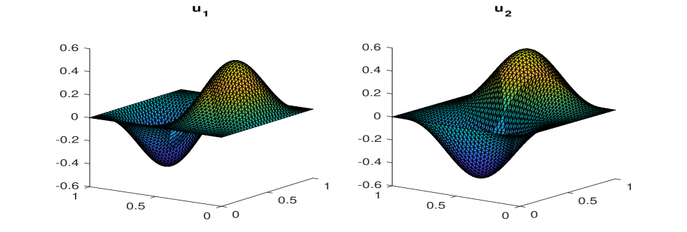
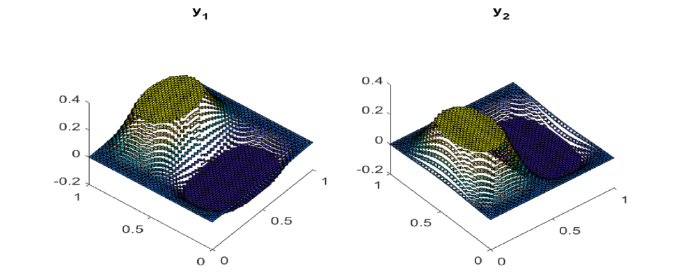
Table 5.1 displays the errors and convergence rates of FE approximations. The linear convergence is observed for error in approximation of state and adjoint state velocity in energy norm, and also for state pressure, adjoint pressure and control variables in -norm. Moreover, we have also observed the quadratic convergence in -norm for state and adjoint state velocity variables.
| CR | CR | CR | CR | CR | ||||||
|---|---|---|---|---|---|---|---|---|---|---|
| 0.2500 | 0.8877 | 0 | 0.9362 | 0 | 0.8888 | 0 | 0.9360 | 0 | 0.0985 | 0 |
| 0.1250 | 0.5350 | 0.73 | 0.3511 | 1.41 | 0.5351 | 0.73 | 0.3510 | 1.41 | 0.0556 | 0.82 |
| 0.0625 | 0.2680 | 0.99 | 0.1682 | 1.06 | 0.2680 | 0.99 | 0.1682 | 1.06 | 0.0296 | 0.91 |
| 0.0312 | 0.1346 | 0.99 | 0.0819 | 1.03 | 0.1346 | 0.99 | 0.0819 | 1.03 | 0.0152 | 0.96 |
| 0.0156 | 0.0674 | 0.99 | 0.0406 | 1.01 | 0.0674 | 0.99 | 0.0406 | 1.01 | 0.0076 | 0.98 |
| 0.0078 | 0.0337 | 0.99 | 0.0202 | 1.00 | 0.0337 | 0.99 | 0.0202 | 1.00 | 0.0038 | 0.99 |
Example 5.2.
This problem is defined on the L-shaped domain, and the solution has a singularity at the origin. It is known that for this problem the uniform refinements will not provide an optimal convergence rate. We have similar observation from Figure 5.5, for uniform refinements convergence rate with respect to the number of degrees of freedom (Ndof) is 0.25 (that is, respect to the mesh-size ). Hence, we have to use the adaptive algorithm to get the optimal convergence. The adaptive algorithm contains a loop: Solve Estimate Mark Refine.
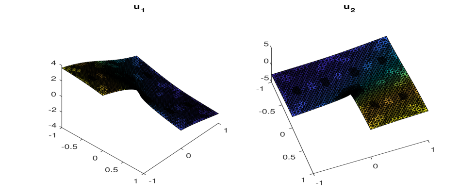
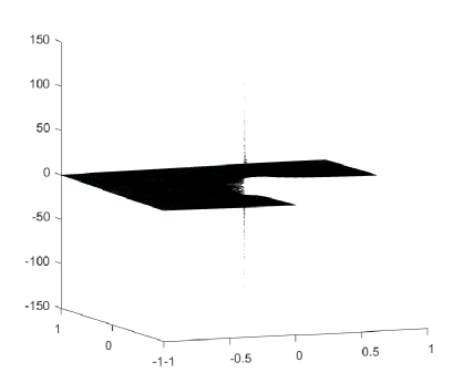
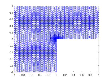
First, we compute the discrete solutions using the primal-dual algorithm. Then, in the second step using the discrete solution we compute the error estimator (as defined in Theorem (4.6)) over each element. We use the Dörlfer marking technique [14] with bulk parameter for the mark step and the newest vertex bisection algorithm for mesh-refinements. Figure 5.3 displays the discrete approximation to velocity and the left-hand side image from Figure 5.4 show the discrete approximation to the pressure . The right-hand image of Figure 5.4 shows adaptive mesh generated from several iterations of adaptive refinements. In figure 5.4, due to a singularity at the origin of the state velocity and pressure variables, more mesh-refinements are observed at the origin, while other refinements are results of the adjoint variable estimator.
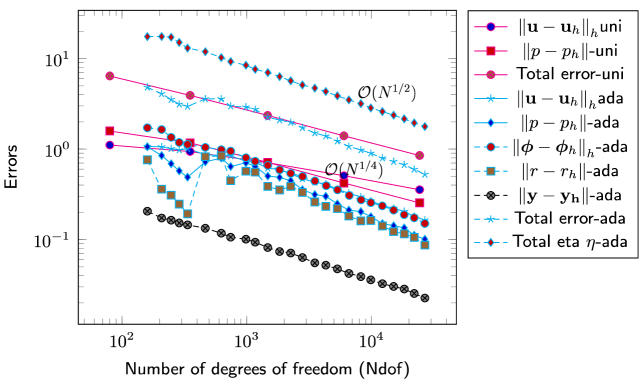
Figure 5.5 depicts convergence rates for errors and estimators with uniform and adaptive refinements. The optimal convergence is achieved using the adaptive algorithm for the error in energy norm in the state and adjoint state velocity approximation, in -norm of control, pressure and adjoint pressure variables. Hence, the optimal convergence for the a posteriori estimator and the total error which is the combination of all errors term as in the left-hand side of (4.6). Here, the optimal convergence means order 0.5 with respect to Ndof.
Conclusions
In this paper, we have developed an abstract framework for discontinuous finite element methods error analysis of both the distributed control and Neumann boundary control problems governed by the stationary Stokes equation, with control constraints. This framework will also work for linear elliptic and mixed optimal control problems with control constraints. The abstract analysis provides the best approximation results, which will be useful in the convergence analysis of adaptive methods and delivers a reliable and efficient a posteriori error estimators. Numerical experiments illustrate the theoretical findings. The results in the article will not directly cover the analysis of nonlinear mixed elliptic optimal control problems; however, they will be useful to analyze the nonlinear problems.
Acknowledgment
The first author gratefully acknowledges financial support from the National Board for Higher Mathematics (NBHM), Government of India.
References
- [1] T. Apel, P. Johannes and A. Rösch. Finite element error estimates for Neumann boundary control problems on graded meshes. Comput. Optim. Appl. 52:3–28, 2012.
- [2] T. Apel, D. Sirch and G. Winkler, Error estimates for control constrained optimal control problems: discretization with anisotropic finite element meshes. Preprint SPP1253-02-06, DFG Priority Program 1253, Erlangen. 2008.
- [3] T. Apel and G. Winkler Optimal control under reduced regularity. Appl. Numer. Math., 59: 2050–2064, 2009.
- [4] S. Badia, R. Codina, T. Gudi and J. Gumaan. Error Analysis of Discontinuous Galerkin Methods for Stokes Problem Under Minimal Regularity. IMA J. Numer. Anal., 34:800–819, 2014.
- [5] P. Bochev and M. Gunzburger. Least-squares finite-element methods for optimization and control problems for the Stokes equations. Comput. Math. Appl., 48:1035–1057, 2004.
- [6] S.C. Brenner. Poincaré-Friedrichs inequalities for piecewise functions, SIAM J. Numer. Anal. 41:306–324, 2003.
- [7] S.C. Brenner and L.R. Scott. The mathematical theory of finite element methods Third edition. Springer-Verlag, New York, 2008.
- [8] C. Carstensen, M. Eigel, R.H.W. Hoppe and C. Löbhard. A review of unified a posteriori finite element error control, Numer. Math. Theory Methods Appl., 5:509–558, 2012.
- [9] C. Carstensen, T. Gudi and M. Jensen. A unifying theorey of a posteriori error control for discontinuous Galerkin FEM. Numer. Math., 112:363–379, 2009.
- [10] E. Casas and J. P. Raymond. Error estimates for the numerical approximation of dirichlet boundary control for semilinear elliptic equations. SIAM J. Control Optim., 45:1586–1611, 2006.
- [11] S. Chowdhury , T. Gudi and A.K. Nandakumaran. A framework for the error analysis of discontinuous finite element methods for elliptic optimal control problems and applications to IP methods., Numer. Funct. Anal. Optim., 36:1388–1419, 2015.
- [12] P. G. Ciarlet. The Finite Element Method for Elliptic Problems. North-Holland, Amsterdam, 1978.
- [13] K. Deckelnick, A. Günther, and M. Hinze. Finite element approximation of Dirichlet boundary control for elliptic PDEs on two and three dimensional curved domains. SIAM J. Numer. Anal., 48:2798–2819, 2009.
- [14] W. Dörfler. A convergent adaptive algorithm for Poisson’s equation, SIAM J. Numer. Anal., 33:1106–1124, 1996.
- [15] D. A. Di Pietro and A. Ern. The mathematical aspects of discontinuous Galerkin methods. Springer-Verlag, Berlin, 2012.
- [16] A. Ern and J-L. Guermond. Theory and practice of finite elements. Springer-Verlag, New York, 2004.
- [17] R. S. Falk. Approximation of a class of optimal control problems with order of convergence estimates. J. Math. Anal. Appl., 44:28–47, 1973.
- [18] T. Geveci. On the approximation of the solution of an optimal control problem governed by an elliptic equation. RAIRO Anal. Numér., 4:313–328, 1979.
- [19] V. Girault and P.-A. Raviart. Finite Element Approximation of the Navier-Stokes Equations. Lecture Notes in Mathematics, vol. 749, Springer, Berlin, 1979.
- [20] T. Gudi. A new error analysis for discontinuous finite element methods for linear elliptic problems. Math. Comp., 79:2169–2189, 2010.
- [21] T. Gudi, N. Nataraj and K. Porwal. An interior penalty method for distributed optimal control problems governed by the biharmonic operator. Comput. Math. Appl., 68:2205–2221, 2014.
- [22] M.D. Gunzburger, L.S. Hou and T. Swobodny. Analysis and finite element approximation of optimal control problems for the stationary Navier-Stokes equations with Dirichlet controls. Math. Model. Numer. Anal., 25:711–748, 1991.
- [23] M. Hintermüller, R.H.W. Hoppe, Y. Iliash and M. Kiewag. An a posteriori error analysis of adaptive finite element methods for distributed elliptic control problems with control constraints. ESAIM Control Optim. Calc. Var., 14:540–560, 2008.
- [24] M. Hintermüller, K. Ito and K. Kunish. The primal-dual active set strategy as a semismooth Newton method. SIAM J. Optim., 13:865-888, 2003.
- [25] M. Hinze. A variational discretization concept in control constrained optimization: The linear-quadratic case. Comput. Optim. Appl., 30:45-61, 2005.
- [26] P. Houston, D. Schautau and T.P. Wihler. Energy norm a posteriori error estimation for mixed discontinuous Galerkin approximations of the Stokes problem. J. Sci. Comput., 22/23:347-370, 2005.
- [27] D. Leykekhman and M. Heinkenschloss. Local error analysis of discontinuous Galerkin methods for advection-dominated elliptic linear-quadratic optimal control problems. SIAM J. Numer. Anal., 4:2012-2038, 2012.
- [28] S. May, R. Rannacher and B. Vexler. Error analysis for a finite element approximation of elliptic dirichlet boundary control problems. SIAM J. Control Optim., 51:2585-2611, 2013.
- [29] C. Meyer and A. Rósch. Superconvergence properties of optimal control problems. SIAM J. Control and Optimization, 43:970–985, 2004.
- [30] J.-C. Nédélec. A new family of mixed finite elements in R3. Numer. Math., 50, 57–81, 1986.
- [31] S. Nicaise and D. Sirch. Optimal control of the Stokes equations: conforming and non-conforming finite element methods under reduced regularity. Comput Optim Appl 49:567–600, 2011.
- [32] G. Of, T. X. Phan and O. Steinbach. An energy space finite element approach for elliptic Dirichlet boundary control problems. Numer. Math., 129:723–748, 2015.
- [33] A. Rösch and Boris Vexler. Optimal Control of the Stokes equations : a priori error analysis for the finite element Discretization with Postprocessing. SIAM J. Numer. Anal., 5:1903–1920, 2006.
- [34] F. Tröltzsch. Optimal control of partial differential equations: Theory, methods and applications. American Mathematical Society, Providence, RI, 2010.
- [35] R. Verfürth. A Review of A Posteriori Error Estimation and Adaptive Mesh-Refinement Techniques. Wiley-Teubner, Chichester, 1995.