Nonlinear topological phase diagram in dimerized sine-Gordon model

Abstract

We investigate the topological physics and the nonlinearity-induced trap phenomenon in a coupled system of pendulums. It is described by the dimerized sine-Gordon model, which is a combination of the sine-Gordon model and the Su-Schrieffer-Heeger model. The initial swing angle of the left-end pendulum may be regarded as the nonlinearity parameter. The topological number is well defined as far as the pendulum is approximated by a harmonic oscillator. The emergence of the topological edge state is clearly observable in the topological phase by solving the quench dynamics starting from the left-end pendulum. A phase diagram is constructed in the space of the swing angle $\xi\pi$ with $|\xi|\leq 1$ and the dimerization parameter $\lambda$ with $|\lambda|\leq 1$. It is found that the topological phase boundary is rather insensitive to the swing angle for $|\xi|\lesssim 1/2$. On the other hand, the nonlinearity effect becomes dominant for $|\xi|\gtrsim 1/2$, and eventually the system turns into the nonlinearity-induced trap phase. Furthermore, when the system is almost dimerized ($\lambda\simeq 1$), coupled standing waves appear and are trapped to a few pendulums at the left-end, forming the dimer phase. Its dynamical origin is the cooperation of the dimerization and the nonlinear term.

Introduction. Topological physics is extensively studied in condensed-matter physicsHasan ; Qi . A topological phase is signaled by the emergence of topological edge states if a sample has a boundary. Now, the target of topological physics is expanded to artificial topological systems such as acousticProdan ; TopoAco ; Berto ; Xiao ; He ; Abba ; Xue ; Ni ; Wei ; Xue2 , mechanicalLubensky ; Chen ; Nash ; Paul ; Sus ; Sss ; Huber ; Mee ; Kariyado ; Hannay ; Po ; Rock ; Takahashi ; Mat ; Taka ; Ghatak ; Wakao , photonicKhaniPhoto ; Hafe2 ; Hafezi ; WuHu ; TopoPhoto ; Ozawa ; Hassan ; Li and electric circuitTECNature ; ComPhys ; Hel ; Lu ; YLi ; EzawaTEC ; Zhao ; EzawaLCR ; EzawaSkin ; Garcia ; Hofmann systems. The merit of artificial topological systems is that system parameters can be finely controlled. In addition, it is possible to make a small sample with clean edges.

Topological physics has been mainly studied in linear systems. Recently, the frontier of the study of topological phases has reached nonlinear systems. Nonlinear effects are naturally introduced in artificial topological systems. In this context, topological physics in nonlinear systems is studied in mechanicalSnee ; PWLo ; MechaRot , photonicLey ; Zhou ; MacZ ; Smi ; Tulo ; Kruk ; NLPhoto ; Kirch , electric circuitHadad ; TopoToda and resonatorZange systems. It is an interesting problem how the topological phases are modified in the presence of the nonlinear term. Furthermore, it is fascinating if there is a transition induced by the nonlinear term.

In this paper, we study topological physics in nonlinear systems analytically and numerically by taking the discrete sine-Gordon model with dimerization. This model is realized by a coupled pendulum system with alternating torsion as illustrated in Fig.1. We give an oscillation only to the left-end pendulum initially, and investigate a quench dynamics how the oscillation propagates to other pendulums. The initial swing angle $\xi\pi$ at the left-end pendulum may be taken as the nonlinearity parameter, where $|\xi|\leq 1$. We explore a phase diagram of the model. Since this model is reduced to the Su-Schrieffer-Heeger (SSH) model in the absence of the nonlinear term, it is natural to expect that the topological phase diagram is valid in the weak nonlinear regime. Indeed, it is possible to define the topological number for $|\xi|\ll 1$ by the first-order perturbation theory with respect to $\xi$. Physically this correspond to the case where the pendulum motion is well approximated by a harmonic oscillator. Beyond the weak nonlinear regime we determine phases by studying a quench dynamics numerically. It is found that the phase boundary is quite insensitive to the nonlinearity parameter for $|\xi|\lesssim 1/2$. The nonlinearity effect becomes dominant for $|\xi|\gtrsim 1/2$, and eventually the system turns into the nonlinearity-induced trap phase.

We have found four phases. First, we have the topological phase, where the oscillation at the left-end pendulum stays as a standing wave. Second, we have the trivial phase, where it propagates into the bulk. Third, the system turns into the trap phase in the strong nonlinear regime, where the oscillation occurs as a perfectly localized standing wave at the left-end pendulum. This is because the interaction between adjacent pendulum is negligible with respect to the nonlinear localization effect. Forth, we find the dimer phase, where coupled standing waves are trapped to a few pendulums at the left-end. Its dynamical origin is the cooperation of the dimerization and the nonlinear term.

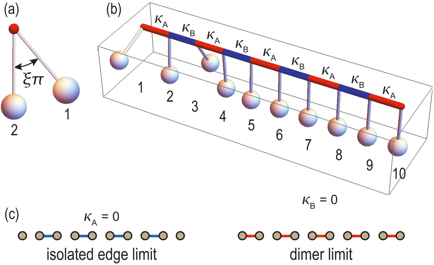
Figure 1: Illustration of coupled pendulums. Adjacent pendulums are connected by a wire which has a restoring force depending on the angle difference. The torsion is alternating as $\kappa_{A}$ and $\kappa_{B}$. The system is described by the dimerized sine-Gordon equation. (a) Horizontal view of the initial condition (11). (b) Bird’s eye’s view of a chain of pendulums in the topological phase, where $g/\kappa=1,$ $\lambda=-0.5$ and $\xi=0.5$. The pendulum at $n=2$ is stationary. (c) Illustration of the isolated edge limit and the dimer limit.

Discrete sine-Gordon model. A typical nonlinear system is the sine-Gordon model described by

$$m\frac{d^{2}\phi}{dt^{2}}=\kappa\frac{\partial^{2}\phi}{\partial x^{2}}-g\sin\phi.$$ (1)

By discretizing it on a one-dimensional chain, we obtain a discrete sine-Gordon modelHirotaDSG ; Orfan , where the equation of motion is given by

$$m\frac{d^{2}\phi_{n}}{dt^{2}}=\kappa\left[\phi_{n+1}+\phi_{n-1}-2\phi_{n}\right]-g\sin\phi_{n}.$$ (2)

It is rewritten in the form of

$$m\frac{d^{2}\phi_{n}}{dt^{2}}+g\sin\phi_{n}-\sum_{nm}M_{nm}\phi_{m}=0,$$ (3)

with the hopping matrix with the coupling $\kappa$,

$$M_{nm}=\kappa\left(\delta_{n,m+1}+\delta_{n,m-1}-2\delta_{n,m}\right).$$ (4)

Eq.(3) is derived from the Lagrangian

$$L=\sum_{n}\left[m\left(\frac{d\phi_{n}}{dt}\right)^{2}+g\cos\phi_{n}\right]+\sum_{nm}M_{nm}\phi_{n}\phi_{m}.$$ (5)

The corresponding Hamiltonian is

$$H=\sum_{n}\left[m\left(\frac{d\phi_{n}}{dt}\right)^{2}-g\cos\phi_{n}\right]-\sum_{nm}M_{nm}\phi_{n}\phi_{m},$$ (6)

which is a conserved energy.

Dimerized sine-Gordon model. We investigate the system where the matrix $M_{nm}$ generates a nontrivial topological structure. Such a matrix is simply given by the SSH model. The equation of motion is given by Eq.(3) together with the hopping matrix

$$M_{nm} = -\left(\kappa_{A}+\kappa_{B}\right)\delta_{n,m}+\kappa_{A}\left(\delta_{2n,2m-1}+\delta_{2m,2n-1}\right)$$ (7)

$$+\kappa_{B}\left(\delta_{2n,2m+1}+\delta_{2m,2n+1}\right).$$

The Lagrangian of the system is given by Eq.(5) with (7), to which we refer as the dimerized sine-Gordon model.

The explicit equations are given by

$$m\frac{d^{2}\phi_{2n-1}}{dt^{2}} = \kappa_{A}\left(\phi_{2n}-\phi_{2n-1}\right)+\kappa_{B}\left(\phi_{2n-2}-\phi_{2n-1}\right)$$ (8)

$$-g\sin\phi_{2n-1},$$

$$m\frac{d^{2}\phi_{2n}}{dt^{2}} = \kappa_{B}\left(\phi_{2n+1}-\phi_{2n}\right)+\kappa_{A}\left(\phi_{2n-1}-\phi_{2n}\right)$$ (9)

$$-g\sin\phi_{2n}.$$

It is convenient to introduce the coupling strength $\kappa$ and the dimerization parameter $\lambda$ by

$$\kappa_{A}=\kappa\left(1+\lambda\right),\quad\kappa_{B}=\kappa\left(1-\lambda\right),$$ (10)

with $|\lambda|\leq 1$.

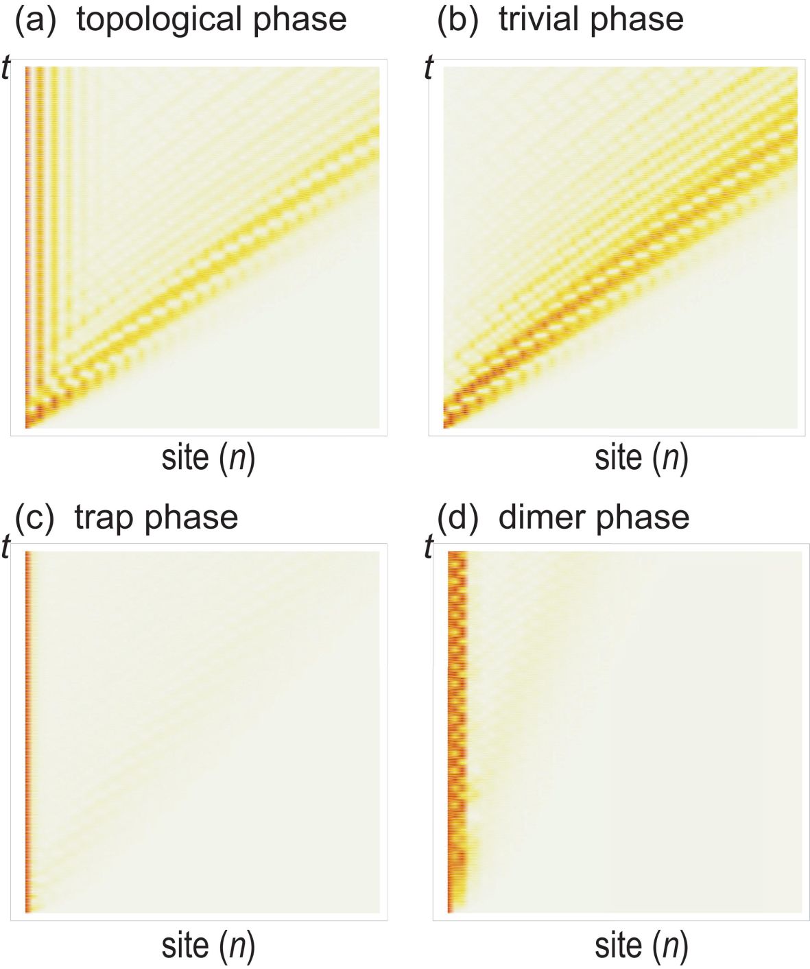
Figure 2: Time evolution of $\phi_{n}$ for (a) the topological phase with $\lambda=-0.25$ and $\xi=0.1$; (b) the trivial phase with $\lambda=0.25$and $\xi=0.1$; (c) the trap phase with $\lambda=0.5$ and $\xi=0.75$; (d) the dimer phase with $\lambda=0.75$ and $\xi=0.5$. We have set $g/\kappa=10$.

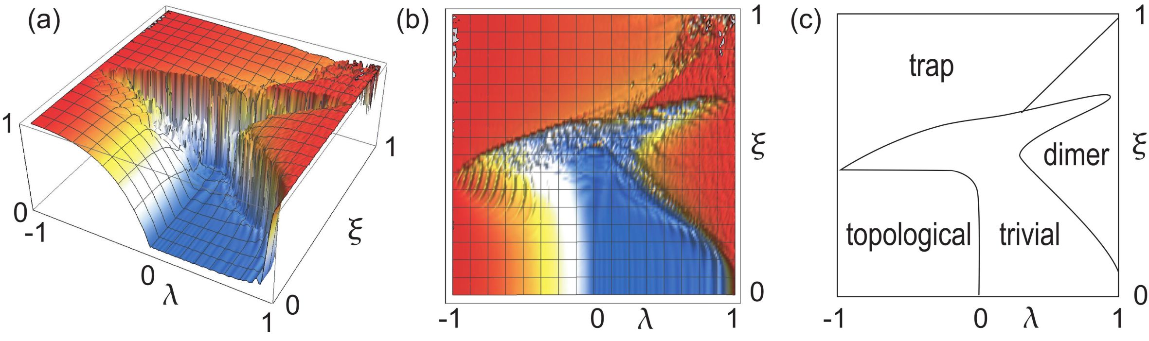
Figure 3: Normalized swing angle $\phi_{1}/\xi\pi$ of the left-end pendulum after enough time as a function of the dimerization $\lambda$ and the initial condition $\xi$. (a) Bird’s eye’s view and (b) top view. We have set $g/\kappa=10$. (c) Schematic illustration of phases.

Mechanical system realization. We discuss how to realize the dimerized sine-Gordon model experimentally. It is realized by a mechanical system shown in Fig.1, where coupled pendulums are connected by wires. Each pendulum rotates perpendicular to the wire direction. The alternating hopping coefficients $\kappa_{A}$ and $\kappa_{B}$ are introduced by the torsion of the wire connecting two pendulums. $M_{nm}$ is a matrix representing the couplings between the $n$-th and $m$-th pendulums. A wire has a restoring force against the force induced by the angle difference between the two adjacent pendulums. $m$ is an inertia moment of the pendulum and $g$ is the gravitational acceleration constant.

Quench dynamics. We analyze a quench dynamics, where we solve the dimerized sine-Gordon equation under the initial condition,

$$\phi_{n}\left(t\right)=\xi\pi\delta_{n,1}\quad\text{and}\quad\dot{\phi}_{n}\left(t\right)=0\quad\text{at}\quad t=0,$$ (11)

where $|\xi|\leq 1$. Namely, in the case of a chain of pendulums, we set the initial angle of the left-end pendulum to be $\xi\pi$ and all the others to be zero as in Fig.1(a). Then, allowing it to move with the zero initial velocity under the gravitational force, we study how the motion propagates along the chain as in Fig.1(b). We discuss later that $\xi$ controls the nonlinearity, and hence we call it the nonlinearity parameter.

We treat the coupling strength $\kappa$, the dimerization parameter $\lambda$ and the nonlinearity parameter $\xi$ as the system parameters. We have studied the quench dynamics for a variety of these parameters. We have found there are four types of solutions numerically, whose typical structures are given in Fig.2.

In Fig.2(a), there are standing waves mainly at the left-end pendulum and weakly at a few adjacent pendulums, and furthermore there are propagating waves into the bulk with a constant velocity. In Fig.2(b), there are only propagating waves into the bulk with a constant velocity. In Fig.2(c), the standing wave is trapped strictly at the left-end pendulum. In Fig.2(d), the standing waves are trapped to a few pendulums at the left-end.

In general, it is impossible to solve the dimerized sine-Gordon equation analytically. Nevertheless, it is possible to obtain analytical results to explain these behaviors.

Topological and trivial phases. First, we make a change of variable, $\phi_{n}=\xi\phi_{n}^{\prime}$, and rewrite Eq.(3) as

$$m\frac{d^{2}\phi_{n}^{\prime}}{dt^{2}}=\sum_{m}M_{nm}\phi_{m}^{\prime}-\frac{g}{\xi}\sin\xi\phi_{n}^{\prime},$$ (12)

with the initial condition

$$\phi_{1}^{\prime}(0)=\pi.$$ (13)

By taking the limit $\xi\rightarrow 0$, Eq.(12) is reduced to a linear equation,

$$m\frac{d^{2}\phi_{n}}{dt^{2}}=\sum_{m}\overline{M}_{nm}\phi_{m},$$ (14)

where we have redefined the hopping matrix as

$$\overline{M}_{nm}\equiv M_{nm}-g\delta_{n,m}.$$ (15)

Actually, it is a very good approximation to set $\sin\xi\phi_{n}^{\prime}\simeq\xi\phi_{n}^{\prime}$ in the vicinity of $\xi=0$. We call such a parameter region the weak nonlinear regime, where the nonlinear equation (3) is well approximated by Eq.(14). Physically, this corresponds to the case where the pendulum is approximated by a harmonic oscillator. Thus, the parameter $\xi$ controls the nonlinearity.

Eq.(14) is the SSH model with a modified matrix $\overline{M}_{nm}$. The SSH model is well known to have a topological and trivial phases. The topological number is the Berry phase defined by

$$\Gamma=\frac{1}{2\pi}\int_{9}^{2\pi}A\left(k\right)dk,$$ (16)

where $A\left(k\right)=-i\left\langle\psi(k)\right|\partial_{k}\left|\psi(k)\right\rangle$ is the Berry connection with $\psi(k)$ the eigenfunction of $\overline{M}\left(k\right)$. Note that the diagonal term in Eq.(15) with (7) does not contribute to the topological charge because the wave function $\psi(k)$ does not depend on the diagonal term. Hence, the present model (14) has the same phases as the SSH model. The system is topological for $\lambda<0$ and trivial for $\lambda>0$ in the weak nonlinear regime.

The topological phase is characterized by the emergence of zero-mode edge states for a finite chain. In the linearized equation (14), the zero-mode edge state is solved as

$$\phi_{2n+1}=\left(-\frac{\kappa_{A}}{\kappa_{B}}\right)^{n}\phi_{1},\quad\quad\phi_{2n}=0.$$ (17)

It has the major component in the left-end pendulum but has components also in a few adjacent pendulums. Now, the initial motion is given only to the left-end pendulum, which is only a part of the zero-mode edge state. This mismatch lets some parts to propagate into the bulk with the velocity $\sim\sqrt{\kappa/m}$, while those within the zero-mode edge state stay as they are, exhibiting standing waves. Thus, this analytic solution well describes the structure made of standing waves and propagating waves, as shown in Fig.2(a), where $\lambda=-0.25$ and $\xi=0.1$.

On the other hand, there is no zero-mode edge state in the trivial phase. Hence, the left-end pendulum motion propagates entirely into the bulk, which well explains the structure made of propagating waves with the velocity $\sim\sqrt{\kappa/m}$ in Fig.2(b), where $\lambda=0.25$ and $\xi=0.1$.

Trap phase. We next study the limit where the nonlinear term is dominant over the hopping term in Eq.(3), where we may approximate it as

$$m\frac{d^{2}\phi_{n}}{dt^{2}}=-g\sin\phi_{n}.$$ (18)

We call such a parameter region the strong nonlinear regime, where the nonlinear equation (3) is well approximated by Eq.(18).

The prominent feature of the strong nonlinear regime is that all equations are perfectly decoupled. Each one is a simple pendulum equation, whose exact solution is given by

$$\phi_{n}=2\sin^{-1}[\alpha_{n}\text{sn}(\omega t,\alpha_{n})],$$ (19)

where sn is the Jacobi elliptic function, $\omega\equiv\sqrt{g/m}$ and $\alpha_{n}$ is determined as $\alpha_{n}=\sin[\phi_{n}\left(0\right)/2]$ in terms of the initial condition $\phi_{n}(0)$. Under the initial condition (11), the left-end pendulum makes a motion described by Eq.(19) with $n=1$ while all other pendulums remain stationary. The pendulum motion is perfectly trapped to the left end of the chain, as explains the structure made of a single standing wave in Fig.2(c), where $\lambda=0.5$ and $\xi=0.75$.

Dimer phase. We finally consider the limit $\lambda=1$, where the system is perfectly dimerized. In this case, the equations of motion are given by

$$m\frac{d^{2}\phi_{1}}{dt^{2}} = \kappa_{A}\left(\phi_{2}-\phi_{1}\right)-g\sin\phi_{1},$$ (20)

$$m\frac{d^{2}\phi_{2}}{dt^{2}} = \kappa_{A}\left(\phi_{1}-\phi_{2}\right)-g\sin\phi_{2}.$$ (21)

By setting $\phi_{2}=-\phi_{1}$, they are combined into one equation

$$m\frac{d^{2}\phi_{1}}{dt^{2}}=-2\kappa_{A}\phi_{1}-g\sin\phi_{1}.$$ (22)

This is solved for $\phi_{1}$ as the inverse function of the integral

$$\int\frac{d\phi_{1}}{\frac{2}{m}\sqrt{E+g\cos\phi_{1}-\kappa_{A}\phi_{1}^{2}}}=t-t_{0},$$ (23)

where

$$E=\frac{m}{2}\dot{\phi}_{1}^{2}-g\cos\phi_{1}+\kappa_{A}\phi_{1}^{2}$$ (24)

is the conserved energy.

However, the initial condition is given by $\phi_{1}=\xi\pi$ and $\phi_{2}=0$, which does not satisfies the condition $\phi_{2}=-\phi_{1}$. It leads to a complicated behavior at the initial stage. Furthermore, the above analysis is correct only in the limit $\lambda=1$. In general, a coupling is present between the dimer and the adjacent pendulum. Numerical calculation shows coupled standing waves trapped to a few pendulums at the left-end in Fig.2(d), where $\lambda=0.75$ and $\xi=0.5$. This is a kind of a pull-in effect in nonlinear systems.

Phase diagram. We have performed a numerical calculation of the quench dynamics for the left-end pendulum in a wide range of system parameters. We show the value of $\phi_{1}$ of the left-end pendulum after enough time as a function of the dimerization $\lambda$ and the initial phase $\xi$ in Fig.3. It presents a phase diagram of the system. We have set $g/\kappa=10$ so that the system belongs to the strong nonlinear regime around $\xi=1$.

We find four distinct phases: 1) the topological phase, 2) the trivial phase, 3) the trap phase and 4) the dimer phase. The distinction between the topological and trivial phases is clear analytically in the weak nonlinear regime ($\xi\simeq 0$). We have found numerically that this topological phase boundary does not change in spite of the increase of the nonlinear term up to $\xi\lesssim 0.5$. On the other hand, there is a nonlinearity-induced trap phase in the strong nonlinear regime ($\xi\simeq 1$). We have found numerically that the trap phase appear even for $\xi\gtrsim 0.6$. There is another phase in the vicinity of $\lambda=1$, which is the dimer phase. We have found numerically that the dimer phase is realized for $\lambda\gtrsim 0.3$ at $\xi\approx 0.5$.

Discussion. We have explored the phase diagram of the dimerized sine-Gordon model by investigating the quench dynamics. The phase diagram is very similar to that of the nonlinear Schrödinger systemsNLPhoto although the models are very different. Indeed, the former is the second-order differential equation with real variables, while the latter is the first-order differential equation with complex variables.

The similarity reveals a universal feature of nonlinear topological systems. The similarity between these models is that there are two competing terms. One is the hopping term governing topological physics in the weak nonlinear regime, and the other is the nonlinear term governing nontopological physics in the strong nonlinear regime. In the weak nonlinear regime, the system is well described by the hopping term and the topological phase boundary remains as it is. On the other hand, in the strong nonlinear limit, the system turns into a nonlinearity-induced trap phase irrespective of the dimerization parameter $\lambda$, because the hopping term does not play a significant role. In addition, there is a dimer phase, where the quench dynamics is trapped to a few pendulums at the left-end.

Our results show that the quench dynamics starting from the edge is a good signal to determine a phase diagram. It is an interesting problem to study various nonlinear systems in the context of topology.

The author is very much grateful to N. Nagaosa for helpful discussions on the subject. This work is supported by the Grants-in-Aid for Scientific Research from MEXT KAKENHI (Grants No. JP17K05490 and No. JP18H03676). This work is also supported by CREST, JST (JPMJCR16F1 and JPMJCR20T2).

References

- (1) M. Z. Hasan and C. L. Kane, Rev. Mod. Phys. 82, 3045 (2010).
- (2) X.-L. Qi and S.-C. Zhang, Rev. Mod. Phys. 83, 1057 (2011).
- (3) E. Prodan and C. Prodan, Phys. Rev. Lett. 103, 248101 (2009).
- (4) Z. Yang, F. Gao, X. Shi, X. Lin, Z. Gao, Y. Chong and B. Zhang, Phys. Rev. Lett. 114, 114301 (2015).
- (5) P. Wang, L. Lu and K. Bertoldi, Phys. Rev. Lett. 115, 104302 (2015).
- (6) M. Xiao, G. Ma, Z. Yang, P. Sheng, Z. Q. Zhang and C. T. Chan, Nat. Phys. 11, 240 (2015).
- (7) C. He, X. Ni, H. Ge, X.-C. Sun,Y.-B. Chen1 M.-H. Lu, X.-P. Liu, L. Feng and Y.-F. Chen, Nature Physics 12, 1124 (2016).
- (8) H. Abbaszadeh, A. Souslov, J. Paulose, H. Schomerus and V. Vitelli, Phys. Rev. Lett. 119, 195502 (2017).
- (9) H. Xue, Y. Yang, F. Gao, Y. Chong and B.Zhang, Nature Materials 18, 108 (2019).
- (10) X. Ni, M. Weiner, A. Alu and A. B. Khanikaev, Nature Materials 18, 113 (2019).
- (11) M. Weiner, X. Ni, M. Li, A. Alu, A. B. Khanikaev, Science Advances 6, eaay4166 (2020).
- (12) H. Xue, Y. Yang, G. Liu, F. Gao, Y. Chong and B. Zhang, Phys. Rev. Lett. 122, 244301 (2019).
- (13) C. L. Kane and T. C. Lubensky, Nature Phys. 10, 39 (2014).
- (14) B. Gin-ge Chen, N. Upadhyaya and V. Vitelli, PNAS 111, 13004 (2014).
- (15) L. M. Nash, D. Kleckner, A. Read, V. Vitelli, A. M. Turner and W. T. M. Irvine, PNAS 112, 14495 (2015).
- (16) J. Paulose, A. S. Meeussen and V. Vitelli, PNAS 112, 7639 (2015).
- (17) R. Susstrunk, S. D. Huber, Science 349, 47 (2015).
- (18) R. Susstrunk and S. D. Huber, Proc. Natl. Acad. Sci. USA 113, E4767 (2016).
- (19) S. D. Huber, Nature Physics 12, 621 (2016).
- (20) A. S. Meeussen, J. Paulose and V. Vitelli, Phys. Rev. X 6, 041029 (2016).
- (21) T. Kariyado and Y. Hatsugai, Sci. Rep. 5, 18107 (2016).
- (22) T. Kariyado and Y. Hatsugai, J. Phys. Soc. Jpn. 85, 043001 (2016).
- (23) H. C. Po, Y. Bahri and A. Vishwanath, Phys. Rev. B 93, 205158 (2016).
- (24) D. Zeb Rocklin, Bryan Gin–ge Chen, Martin Falk, Vincenzo Vitelli, and T. C. Lubensky, Phys. Rev. Lett. 116, 135503 (2016).
- (25) Y. Takahashi, T. Kariyado and Y. Hatsugai, New J. Phys. 19, 035003 (2017).
- (26) K. H. Matlack, M. Serra-Garcia, A. Palermo, S. D. Huber and C. Daraio, Nature Mat. 17, 323 (2018).
- (27) Y. Takahashi, T. Kariyado and Y. Hatsugai, Phys. Rev. B 99, 024102 (2019).
- (28) A. Ghatak, M. Brandenbourger, J. van Wezel and C. Coulais, Proc. Natl. Ac. Sc. U.S.A. 117, 29561 (2020).
- (29) H. Wakao, T. Yoshida, H. Araki, T. Mizoguchi and Y. Hatsugai, Phys. Rev. B 101, 094107 (2020).
- (30) A. B. Khanikaev, S. H. Mousavi, W.-K. Tse, M. Kargarian, A. H. MacDonald, G. Shvets, Nature Materials 12, 233 (2013).
- (31) M. Hafezi, E. Demler, M. Lukin, J. Taylor, Nature Physics 7, 907 (2011).
- (32) M. Hafezi, S. Mittal, J. Fan, A. Migdall, J. Taylor, Nature Photonics 7, 1001 (2013).
- (33) L.H. Wu and X. Hu, Phys. Rev. Lett. 114, 223901 (2015).
- (34) L. Lu. J. D. Joannopoulos and M. Soljacic, Nature Photonics 8, 821 (2014).
- (35) T. Ozawa, H. M. Price, A. Amo, N. Goldman, M. Hafezi, L. Lu, M. C. Rechtsman, D. Schuster, J. Simon, O. Zilberberg and L. Carusotto, Rev. Mod. Phys. 91, 015006 (2019).
- (36) A. E. Hassan, F. K. Kunst, A. Moritz, G. Andler, E. J. Bergholtz, M. Bourennane, Nature Photonics 13, 697 (2019).
- (37) M. Li, D. Zhirihin, D. Filonov, X. Ni, A. Slobozhanyuk, A. Alu and A. B. Khanikaev, Nature Photonics 14, 89 (2020).
- (38) S. Imhof, C. Berger, F. Bayer, J. Brehm, L. Molenkamp, T. Kiessling, F. Schindler, C. H. Lee, M. Greiter, T. Neupert, R. Thomale, Nat. Phys. 14, 925 (2018).
- (39) C. H. Lee , S. Imhof, C. Berger, F. Bayer, J. Brehm, L. W. Molenkamp, T. Kiessling and R. Thomale, Communications Physics, 1, 39 (2018).
- (40) T. Helbig, T. Hofmann, C. H. Lee, R. Thomale, S. Imhof, L. W. Molenkamp and T. Kiessling, Phys. Rev. B 99, 161114 (2019).
- (41) Y. Lu, N. Jia, L. Su, C. Owens, G. Juzeliunas, D. I. Schuster and J. Simon, Phys. Rev. B 99, 020302 (2019).
- (42) Y. Li, Y. Sun, W. Zhu, Z. Guo, J. Jiang, T. Kariyado, H. Chen and X. Hu, Nat. Com. 9, 4598 (2018).
- (43) M. Ezawa, Phys. Rev. B 98, 201402(R) (2018).
- (44) E. Zhao, Ann. Phys. 399, 289 (2018).
- (45) M. Ezawa, Phys. Rev. B 99, 201411(R) (2019).
- (46) M. Ezawa, Phys. Rev. B 99, 121411(R) (2019).
- (47) M. Serra-Garcia, R. Susstrunk and S. D. Huber, Phys. Rev. B 99, 020304 (2019).
- (48) T. Hofmann, T. Helbig, C. H. Lee, M. Greiter, R. Thomale, Phys. Rev. Lett. 122, 247702 (2019).
- (49) D. D. J. M. Snee, Y.-P. Ma, Extreme Mechanics Letters 100487 (2019).
- (50) P.-W. Lo, K. Roychowdhury, B. G.-g. Chen, C. D. Santangelo, C.-M. Jian, M. J. Lawler, Phys. Rev. Lett. 127, 076802 (2021).
- (51) M. Ezawa, arXiv:2108.09634.
- (52) Lukas J. Maczewsky, Matthias Heinrich, Mark Kremer, Sergey K. Ivanov, Max Ehrhardt, Franklin Martinez, Yaroslav V. Kartashov, Vladimir V. Konotop, Lluis Torner, Dieter Bauer, Alexander Szameit, Science 370, 701 (2010).
- (53) D. Leykam and Y. D. Chong, Phys. Rev. Lett. 117, 143901 (2016).
- (54) X. Zhou, Y. Wang, D. Leykam and Y. D. Chong, New J. Phys. 19, 095002 (2017).
- (55) S. Kruk, A. Poddubny, D. Smirnova, L. Wang, A. Slobozhanyuk, A. Shorokhov, I. Kravchenko, B. Luther-Davies and Y. Kivshar, Nature Nanotechnology 14, 126 (2019).
- (56) D. Smirnova, D. Leykam, Y. Chong and Y. Kivshar, Applied Physics Reviews 7, 021306 (2020).
- (57) T. Tuloup, R. W. Bomantara, C. H. Lee and J. Gong, Phys. Rev. B 102, 115411 (2020).
- (58) M. Ezawa, arXiv:2110.06578.
- (59) M. S. Kirsch, Y. Zhang, M. Kremer, L. J. Maczewsky, S. K. Ivanov, Y. V. Kartashov, L. Torner, D. Bauer, A. Szameit and M. Heinrich, Nature Physics 17, 995 (2021).
- (60) Y. Hadad, J. C. Soric, A. B. Khanikaev, and A. Alù, Nature Electronics 1, 178 (2018).
- (61) M. Ezawa, cond-mat/arXiv:2105.10851.
- (62) F. Zangeneh-Nejad and R. Fleury, Phys. Rev. Lett. 123, 053902 (2019).
- (63) R. Hirota, J. Phys. Soc. Jpn, 43, 2079 (1977).
- (64) S. J. Orfanidis, Phys. Rev. B 18, 3822 (1978).