15th International Symposium on Radiative Corrections:
Applications of Quantum Field Theory to Phenomenology,
FSU, Tallahasse, FL, USA, 17-21 May 2021 10.21468/SciPostPhysProc.?

Abstract

The loop-tree duality (LTD) has become a novelty alternative to bootstrap the numerical evaluation of multi-loop scattering amplitudes. It has indeed been found that Feynman integrands, after the application of LTD, display a representation containing only physical information, the so-called causal representation. In this talk, we discuss the all-loop causal representation of multi-loop Feynman integrands, recently found in terms of features that describe a loop topology, vertices and edges. Likewise, in order to elucidate the numerical stability in LTD integrands, we present applications that involve numerical evaluations of two-loop planar and non-planar triangles with presence of several kinematic invariants.

 

1 Introduction & Motivation

In this contribution, we report on the all-loop causal representation of multi-loop scattering amplitudes, recently proposed in Ref. [1] and automated in the Mathematica package Lotty [2]. In this representation, that manifestly displays the causality of scattering amplitudes [3], the structure of Feynman integrands is cast only by physical singularities, which, within our approach, are usually referred to as causal propagators [4, 5, 6, 7]. Alternative approaches that aim to the generation of integrands displaying only physical singularities have also been discussed in this conference [8, 9, 10].

Interestingly, the causal representation, obtained as by-product of the novel formulation of the loop-tree duality (LTD) formalism [5], has allowed to have a complete understanding on the structure of multi-loop integrands, regardless of the loop order. In particular, since LTD relies on the direct application of the Cauchy residue theorem on the energy component of the loop momenta [11, 12, 13, 14, 15, 16, 17, 4, 5, 18, 19, 20, 21, 22, 23, 24, 25, 8, 26, 27], causal integrands are expressed in terms of on-shell energies, whose functional structure turns out to be equivalent to the integrands obtained from the Old-Fashioned-Perturbation theory (OFPT) [28, 29]. However, by performing a term-by-term comparison between both approaches, it turns out that the causal representation turns out to be more compact than OFPT, which is due to redundant terms that cancel pairwise in the latter, as observed in Ref. [8] of one-loop scalar integrands.

In view of the structure of causal integrands obtained from LTD in Ref. [6], we notice several similarities when computing integrands whose loop topologies have the same number of vertices but differ on the number of edges. This observation promoted to a study in which causal integrands can be directly generated by means of the latter features and completely overcome the application of LTD. In order to carry out this study, we systematically consider all causal (or threshold) singularities of a given loop topology and organise them according to their compatibility. Likewise, as it was point in Ref. [1], the classification of loop topologies by vertices and edges, as well as the generation of causal integrands, corresponds to a consequence of the well-known Steinmann relations [30, 31, 32, 33, 34, 35, 36, 37] and allowed us to provide a conjecture for the representation of all-loop Feynman integrands. Steinmann relations have been considered in recent works [38, 39, 40, 41, 42] that aim at bootstrapping analytic structure of multi-loop scattering amplitudes.

Furthermore, inspired by the recent developments of LTD to numerically evaluate multi-loop Feynman integrals and keep understanding mathematical properties to causal integrands, we provided the publicly Mathematica package Lotty [2] that illustrates and automates the generation of dual and causal integrands, allowing, in this way, to provide the scientific community with alternative strategies to overcome the obstacles in the calculation of multi-loop scattering amplitudes [43, 44, 45].

This contribution is organised as follows. In Sec. 2 we briefly remark the main features of the causal representation of multi-loop scattering amplitudes. Then, in Sec. 3, we recall numerical stability and numerical integration of causal integrands. Then, in Sec. 4, we draw a summary of the talk and discuss future directions.

2 All-loop causal representation of Feynman integrands

In order to explicitly illustrate the causal representation of multi-loop Feynman integrands, let us consider, for the sake of simplicity, the most general loop topology built from five vertices and all possible connections among edges (or internal lines). A pictorial representation of this six-loop topology is depicted in Fig. 1, in which grey lines do not cross among themselves. Hence, taking into account this topology, one can consider a five-point six-loop Feynman integral with ten internal lines,

$$\mathcal{A}_{5}^{\left(6\right)}\left(1,2,\ldots,10\right) =\int_{\ell_{1},\ldots,\ell_{6}}\mathcal{N}\left(\left\{\ell_{i}\right\}_{6},\left\{p_{j}\right\}_{5}\right)\times G_{F}\left(1,\ldots,10\right)\,,$$ (1)

where $\int_{\ell_{s}}\equiv-\imath\mu^{4-d}\int d^{d}\ell_{s}/\left(2\pi\right)^{d}$ and Feynman propagators $G_{F}$ are compactly represented as follows,

$$G_{F}\left(1,\ldots,r\right) =\prod_{i=1}^{r}\left(G_{F}\left(q_{i}\right)\right)^{\alpha_{i}}\,,$$ (2)

where $\alpha_{i}$ are powers of the propagators and, motivated by LTD, one explicitly pulls out the dependence on the energy components of the loop momenta in each internal line,

$$G_{F}\left(q_{i}\right) =\frac{1}{q_{i}^{2}-m_{i}^{2}+\imath 0}=\frac{1}{\left(q_{i,0}+q_{i,0}^{\left(+\right)}\right)\left(q_{i,0}-q_{i,0}^{\left(+\right)}\right)}\,.$$ (3)

The latter corresponds to the usual Feynman propagator of a one single particle, with $m_{i}$ its mass, $+\imath 0$ the infinitesimal imaginary Feynman prescription and,

$$q_{i,0}^{\left(+\right)} =\sqrt{\boldsymbol{q}_{i}^{2}+m_{i}^{2}-\imath 0}\,,$$ (4)

the on-shell energy of the loop momentum $q_{i}$ written in terms of the spatial components $\boldsymbol{q}_{i}$.

Figure 1: Multi-loop topology with five vertices and ten internal lines.

Then, to describe the loop topology of Fig. 1, we work with the propagators,

$$q_{i}= \begin{cases}\ell_{i},\,&i=1,\ldots,6\\ \ell_{1}-\ell_{4}-\ell_{5}-p_{1},&i=7\\ \ell_{2}-\ell_{1}-\ell_{6}-p_{2},&i=8\\ \ell_{3}-\ell_{2}+\ell_{5}-p_{3},&i=9\\ \ell_{4}-\ell_{3}+\ell_{6}-p_{4}&i=10\end{cases}\quad\,,$$ (5)

in which, after applying LTD, one recognises the set of causal propagators,

$$\lambda_{1}^{\pm}=q_{\left(1,4,5,7\right),0}^{\left(+\right)}\pm p_{1,0}\,, \lambda_{12}^{\pm}=q_{\left(2,4,5,6,7,8\right),0}^{\left(+\right)}\pm p_{12,0}\,, \lambda_{24}^{\pm}=q_{\left(1,2,3,4,8,10\right),0}^{\left(+\right)}\pm p_{24,0}\,,$$

$$\lambda_{2}^{\pm}=q_{\left(1,2,6,8\right),0}^{\left(+\right)}\pm p_{2,0}\,, \lambda_{13}^{\pm}=q_{\left(1,2,3,4,7,9\right),0}^{\left(+\right)}\pm p_{13,0}\,, \lambda_{35}^{\pm}=q_{\left(2,3,5,7,8,10\right),0}^{\left(+\right)}\pm p_{35,0}\,,$$

$$\lambda_{3}^{\pm}=q_{\left(2,3,5,9\right),0}^{\left(+\right)}\pm p_{3,0}\,, \lambda_{23}^{\pm}=q_{\left(1,3,5,6,8,9\right),0}^{\left(+\right)}\pm p_{23,0}\,, \lambda_{34}^{\pm}=q_{\left(2,4,5,6,9,10\right),0}^{\left(+\right)}\pm p_{34,0}\,,$$

$$\lambda_{4}^{\pm}=q_{\left(3,4,6,10\right),0}^{\left(+\right)}\pm p_{4,0}\,, \lambda_{45}^{\pm}=q_{\left(3,4,6,7,8,9\right),0}^{\left(+\right)}\pm p_{45,0}\,, \lambda_{25}^{\pm}=q_{\left(1,2,6,7,9,10\right),0}^{\left(+\right)}\pm p_{25,0}\,,$$

$$\lambda_{5}^{\pm}=q_{\left(7,8,9,10\right),0}^{\left(+\right)}\pm p_{5,0}\,, \lambda_{14}^{\pm}=q_{\left(1,3,5,6,7,10\right),0}^{\left(+\right)}\pm p_{14,0}\,, \lambda_{15}^{\pm}=q_{\left(1,4,5,8,9,10\right),0}^{\left(+\right)}\pm p_{15,0}\,.$$ (6)

The causal representation of a topology built from five vertices is expected to admit the decomposition in terms of the following summands,

$$\frac{1}{\lambda_{i}^{h_{i}}\lambda_{j}^{h_{j}}\lambda_{k}^{h_{k}}\lambda_{l}^{h_{l}}}\,,$$ (7)

where $i,j,k,l\in\{1,2,3,4,5,12,13,14,15,23,24,25,34,35\}$ and $h_{\{i,j,k,l\}}\in\{+,-\}$. Nevertheless, not all products of $\lambda_{i}$’s in (6) will appear in the representation, since there will be products of two $\lambda_{i}^{\pm}$’s, that cannot appear because of the incompatible alignment of internal and external momenta. To illustrate this subtlety, let us consider a possible entanglement between $\lambda_{12}^{\pm}$, $\lambda_{14}^{\pm}$ and $\lambda_{12}^{\pm}$, $\lambda_{34}^{\pm}$. In Fig. 2 (left), we note that the causal thresholds $\lambda_{12}^{\pm}$, $\lambda_{14}^{\pm}$ cannot be considered together when providing a candidate for the causal representation, whereas, $\lambda_{12}^{\pm}$, $\lambda_{34}^{\pm}$, in Fig. 2 (right), appear with combinations of other $\lambda_{i}^{\pm}$’s. The very same analysis can be applied to tuples of length three and four.

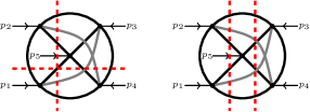
Figure 2: Loop topologies with (left:) two overlapped and (right:) two entangled thresholds.

Interestingly, the above-mentioned features of overlapped and entangled causal thresholds may be related to Steinmann relations, since they state that double discontinuities in overlapping cuts vanish,

$$\text{Disc}_{s_{I}}\left(\text{Disc}_{s_{J}}\mathcal{A}_{N}^{\left(L\right)}\right)=0\,,\quad\text{where }\begin{cases}I\not\subset J\\ J\not\subset I\end{cases}\,,$$ (8)

where $\text{Disc}_{s_{I}}\mathcal{A}_{N}^{\left(L\right)}$ represents the discontinuity of the scattering amplitude (or Feynman integral) of Eq. (1) at the kinematic invariant $s_{I}=\left(\sum_{i\in I}p_{i}\right)^{2}$ generated by the external momenta that belong to the set $I$. A naive interpretation of the Steinmann relations within our framework may be given by promoting the kinematic invariants $s_{I}$ to the sum of energies of external momenta present in the causal propagators.

Hence, by constructing an Ansatz that accounts for the Steinmann relations and reconstructing the analytic expressions for the causal integrand by means of finite fields arithmetic [46, 47, 48, 49], we find for the six-loop five-point scalar integral,

$$\mathcal{A}_{5}^{\left(6\right)}=\int_{\ell_{1},\ldots,\ell_{6}}\frac{1}{x_{10}}\sum_{\begin{subarray}{c}i=1\\ j=i+1\end{subarray}}^{5}\ \sum_{\begin{subarray}{c}k=1\\ l=k+1\\ k,l\neq i,j\end{subarray}}^{5}L_{ij}^{+}\,L_{kl}^{-}\,, L_{ij}^{\pm}=\frac{1}{\lambda_{ij}^{\pm}}\left(\frac{1}{\lambda_{i}^{\pm}}+\frac{1}{\lambda_{j}^{\pm}}\right)\,,$$ (9)

with $x_{n}=\prod_{i=1}^{n}2\,q_{i,0}^{\left(+\right)}$.

Notice that, in view of this very compact structure of the causal representation of a six-loop integrand with five vertices, we proposed in Ref. [1] an algorithm to generate causal representation of topologies constructed from $k+2$ cusps. In fact, due to symmetry in the structure of topologies when all possible connections, edges, between vertices are considered, we conjectured a close formula when all possible edges are taken into account,

$$\mathcal{F}_{L+k}= \sum_{\begin{subarray}{c}i_{1}\ll i_{N_{i}}\\ j_{1}\ll j_{N_{j}}\end{subarray}}^{k+2}\Omega_{\vec{i}}^{\vec{j}}\ L_{i_{1}i_{2}\ldots i_{N_{i}}}^{+}L_{j_{1}j_{2}\ldots j_{N_{j}}}^{-}\,,$$ (10)

with,

$$\Omega_{\vec{i}}^{\vec{j}} =\begin{cases}1&\text{If }\vec{i}\cap\vec{j}=\emptyset\\ 0&\text{otherwise}\end{cases}\,,$$ (11)

where $\vec{i}=\{i_{1},i_{2},\ldots,i_{N_{i}}\}$, $\vec{j}=\{j_{1},j_{2},\ldots,j_{N_{j}}\}$, $i_{1}\ll i_{N_{i}}$ is the lexicographic ordering $i_{1}<i_{2}<\cdots<i_{N_{i}}$, $N_{i}=\left[k/2\right]+1$ and $N_{j}=k-\left[k/2\right]$. The functions $L_{ijk\ldots}^{\pm}$ contain the causal information of the integrand,

$$L_{i_{1}i_{2}\ldots i_{N}}^{\pm}=\frac{1}{\lambda_{i_{1}i_{2}\ldots i_{N}}^{\pm}}\sum_{\begin{subarray}{c}j_{1}\ll j_{N-1}\\ \vec{j}\subset\vec{i}\end{subarray}}L_{j_{1}j_{2}\ldots j_{N-1}}^{\pm}\,, L_{i_{1}}^{\pm}=\frac{1}{\lambda_{i_{1}}^{\pm}}\,.$$ (12)

The close formula (10), together with the definitions of $L^{\pm}$, have been implemented in the built-in routines of the Mathematica package Lotty (see Sec. 3).

On top of decomposition (10), we would like to remark that an extensive study of various representations of scattering amplitudes, including the ones presented in this talk (LTD and causal), are currently under consideration [50], where we elucidate a clear pattern to go from one representation to another along the lines of Ref. [51].

3 Numerical evaluation of Feynman integrals

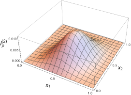
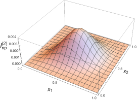
Figure 3: Numerical stability of causal integrands of two-loop planar (left) and non-planar (right) scalar triangles as a function of $x_{1}$ and $x_{2}$ with fixed values for the angles $\theta_{ij}$.

In Refs. [2], we provided the Mathematica package Lotty that automates dual and causal representation of LTD along the lines of Refs. [5] and [1], respectively. This package is publicly available and can be downloaded from the Bitbucket repository:

$$\textrm{\href https://bitbucket.org/wjtorresb/lotty/src/master/}\,.$$

The main motivation to provide this automation was to give the scientific community with an illustrative and pedestrian overview of LTD by means of a Mathematica package. In effect, to recreate the advantage of employing the causal representation of multi-loop scattering amplitudes, we provide the evaluation of planar ($I_{\text{p}}^{(2)}$) and non-planar ($I_{\text{np}}^{(2)}$) three-point integrals at two loops.

Furthermore, because of the causal representation of multi-loop scalar integrands, conjectured in Ref. [1] and briefly summarised in Sec. 2, one can simply make use of the built-in Lotty routine AllCausal and get the most compact representation of the latter in terms of physical singularities,

• AllCausal[5]

•   (L[-][{3,4}] + L[-][{3,5}] + L[-][{4,5}]) L[+][{1,2}]+ (L[-][{2,4}] + L[-][{2,5}] + L[-][{4,5}]) L[+][{1,3}]+ (L[-][{2,3}] + L[-][{2,5}] + L[-][{3,5}]) L[+][{1,4}]+ (L[-][{2,3}] + L[-][{2,4}] + L[-][{3,4}]) L[+][{1,5}]+ (L[-][{1,4}] + L[-][{1,5}] + L[-][{4,5}]) L[+][{2,3}]+ (L[-][{1,3}] + L[-][{1,5}] + L[-][{3,5}]) L[+][{2,4}]+ (L[-][{1,3}] + L[-][{1,4}] + L[-][{3,4}]) L[+][{2,5}]+ (L[-][{1,2}] + L[-][{1,5}] + L[-][{2,5}]) L[+][{3,4}]+ (L[-][{1,2}] + L[-][{1,4}] + L[-][{2,4}]) L[+][{3,5}]+ (L[-][{1,2}] + L[-][{1,3}] + L[-][{2,3}]) L[+][{4,5}]

where, as mentioned in Sec. 2, each $L[\pm][\ldots]$ is expressed in terms of physical singularities only. Besides, to explicitly represent causal representations for planar and non-planar triangles in terms of on-shell energies, one can yet make use of the additional Lotty routines: RefineCausal and Lamb2qij.

Let us remark that within our automation in Mathematica we are not intending to provide a full numerical integration of multi-loop Feynman integrals. Moreover, we can profit from the latter and naively integrate our causal integrands through the built-in function of Lotty for the change of variables, e.g. a two-loop integrand in $d=4$ dimensions:

• dim = 4;  (* set the dimension *)LoopMom = {l1, l2};(* list of loop momenta *)

• LoopToSC[LoopMom, dim]meassure[LoopMom, dim]intvars[LoopMom, dim, "MaxValueR"->max]

• {l1 -> {r1 Cos[$\displaystyle\theta$11], r1 Cos[$\displaystyle\theta$12] Sin[$\displaystyle\theta$11], r1 Sin[$\displaystyle\theta$11] Sin[$\displaystyle\theta$12] }, l2 -> {r2 Cos[$\displaystyle\theta$21], r2 Cos[$\displaystyle\theta$22] Sin[$\displaystyle\theta$21], r2 Sin[$\displaystyle\theta$21] Sin[$\displaystyle\theta$22] } }

• $\displaystyle\text{r1}^{\text{2}}$ $\displaystyle\text{r2}^{\text{2}}$ Sin[$\displaystyle\theta$11] Sin[$\displaystyle\theta$21]

• {{r1,0,max}, {r2,0,max}, {$\displaystyle\theta$11,0,$\displaystyle\pi$}, {$\displaystyle\theta$12,0, 2$\displaystyle\pi$}, {$\displaystyle\theta$21,0,$\displaystyle\pi$}, {$\displaystyle\theta$22,0,2$\displaystyle\pi$}}

where, by default in the integration limits of each radius, "MaxValueR"->$10^{5}$. However, to avoid considering the integration domain $[0,\infty)$, one can map $[0,\infty)$ to the segment $(0,1]$, with the change of variables, $r_{i}=(1-x_{i})/x_{i}$ . Additionally, expressions for on-shell energies ($q_{i,0}^{(+)}$) can be also generated by Lotty, taking into account the momentum components of the external kinematics. For instance, in the three-point loop topology, one may choose, without loss of generality, the center-of-mass frame (COMF),

$$p_{1}^{\mu}=E_{\text{cm}}/2\{1,1,0,0\} p_{2}^{\mu}=E_{\text{cm}}/2\{1,-1,0,0\}\,,$$ (13)

where $E_{\text{cm}}$ is the energy of COMF. In the two-loop planar triangle, this amounts to,

• {$\displaystyle\text{q[1]}_{\text{0}}^{\text{(+)}}$ ->  $\displaystyle\sqrt{\text{$\displaystyle\text{r1}^{\text{2}}$\ +\ $\displaystyle\text{m[1]}^{\text{2}}$}}$, $\displaystyle\text{q[2]}_{\text{0}}^{\text{(+)}}$ -> $\displaystyle\frac{\text{1}}{\text{2}}$$\displaystyle\sqrt{\text{$\displaystyle\text{Ecm}^{\text{2}}$\ +\ 4\ Ecm\ r1\ Cos[$\displaystyle\theta$11]\ +\ 4\ ($\displaystyle\text{r1}^{\text{2}}$\ +\ $\displaystyle\text{m[2]}^{\text{2}}$)}}$, $\displaystyle\text{q[3]}_{\text{0}}^{\text{(+)}}$ ->  $\displaystyle\sqrt{\text{$\displaystyle\text{r1}^{\text{2}}$\ +\ $\displaystyle\text{m[3]}^{\text{2}}$}}$, $\displaystyle\text{q[4]}_{\text{0}}^{\text{(+)}}$ ->  $\displaystyle\sqrt{\text{$\displaystyle\text{r2}^{\text{2}}$\ +\ $\displaystyle\text{m[4]}^{\text{2}}$}}$, $\displaystyle\text{q[5]}_{\text{0}}^{\text{(+)}}$ ->  $\displaystyle\sqrt{\text{$\displaystyle\text{r2}^{\text{2}}$\ +\ $\displaystyle\text{m[5]}^{\text{2}}$}}$, $\displaystyle\text{q[6]}_{\text{0}}^{\text{(+)}}$ ->  $\displaystyle\sqrt{\text{$\displaystyle\text{r1}^{\text{2}}$+$\displaystyle\text{r2}^{\text{2}}$+$\displaystyle\text{m[6]}^{\text{2}}$+2r1r2\ (Cos[$\displaystyle\theta$11]Cos[$\displaystyle\theta$21]\ +\ Cos[$\displaystyle\theta$12-$\displaystyle\theta$22]Sin[$\displaystyle\theta$11]Sin[$\displaystyle\theta$21])}}$ }

The numerical stability of causal integrands for planar and non-planar two-loop triangles in terms of the compactified variable $x_{i}$ and angles $\theta_{ij}$ is displayed in Fig. 3.

	Planar triangle		Non-planar triangle
$\frac{s}{m^{2}}$	LTD ($10^{-6}$)	SecDec 3.0 ($10^{-6}$)	LTD ($10^{-6}$)	SecDec 3.0 ($10^{-6}$)
$-\frac{1}{4}$	9.48(5)	9.4647(9)	4.461(3)	4.4606(4)
$-1$	8.10(5)	8.0885(8)	4.101(3)	4.1012(4)
$-\frac{9}{4}$	6.49(3)	6.4760(6)	3.627(5)	3.6276(3)
$-4$	5.02(2)	5.0188(5)	3.15(5)	3.1334(3)
$+\frac{1}{4}$	10.68(6)	10.651(1)	4.743(3)	4.7436(4)
$1$	13.11(8)	13.070(1)	5.259(3)	5.2590(5)
$+\frac{9}{4}$	20.81(1)	20.748(2)	6.533(3)	6.5331(6)
$+\frac{25}{16}$	15.74(9)	15.700(1)	5.748(3)	5.7474(6)

Table 1: Numerical integration with NIntegrate of planar and non-planar two-loop triangles in the causal representation. The values of integrations are compared with SecDec 3.0.

Hence, one can naively make use of the built-in Mathematica routine NIntegrate to integrate our expressions. A few representative results are collected in Table 1, where we emphasise that no optimisation or educated use of the latter routine is carried out. Likewise, to compare our numerical integrations, we make use of publicly automated codes that evaluates the latter by means of the sector decomposition algorithm [52, 53, 54, 55], SecDec 3.0 [56] and Fiesta 4.2 [57].

In view of the interesting compact structure obtained for multi-loop causal integrands, it is worth dedicating further studies to numerical integrations. The natural extension is having a stable integrator that systematically allows to improve precision in evaluations. To this end, one can rely on publicly available implementations for multi-dimensional numerical integrations, e.g. Cuba library [58, 59], and interface it with Lotty to, thus, keep control of the numerical evaluation from the symbolic side [60].

4 Discussion

The loop-tree duality (LTD) formulation has become a novel alternative approach to numerically evaluate multi-loop scattering amplitudes, which in the current era is one of the main obstacles to go further in theoretical predictions. However, dual integrands, or expressions obtained from the direct application of LTD on multi-loop Feynman integrands, are not the ultimate representation, since it yet contains so-called spurious contributions but they can yet be employed to understand LTD decompositions in scattering amplitudes, regardless of the loop order [5].

In this talk, we introduced the concept of causal representation of multi-loop scattering amplitudes, which in a nutshell corresponds to having an integrand displaying only physical singularities. Remarkably, the Old-Fashioned-Perturbation theory (OFPT) aims at displaying a very same pattern for Feynman integrands. However, these OFPT integrands turn out to be explicitly classified according to number of vertices and not accounting for number of edges (or internal lines). In the causal representation, generated from LTD, the situation is slightly different, the structure of causal integrands accounts for both vertices and edges. In effect, as elucidated in Ref. [1], it is possible to generate a representation for all-loop scalar integrands, by accounting for the features of the loop topology, given by vertices and edges.

Furthermore, we remarked that the all-loop causal representation for multi-loop Feynman integrands has been conjectured by keeping into account the Steinmann relations. Moreover, to give support to this conjecture, we provided a Mathematica implementation of the latter by means of the automated package Lotty [2], in which a direct comparison between LTD and causal integrands can straightforwardly be performed.

Different representations of scattering amplitudes are currently appearing, the main question to address is: what is then the best representation? Perhaps, there is no a unique answer and, on the contrary, one could think of asking further and being more specific. For instance, what would we like to extract from a given representation? In this case, one could put on the table all available representations and extract the most convenient one for the desirable study [50].

In the spirit of profiting from the compact structure of the causal representation of multi-loop Feynman integrands, we observed a smooth behaviour in their numerical evaluation. Therefore, to integrate the latter, this is a very important insight since one can only focus on the treatment of physical singularities. We illustrated that by simply using the built-in Mathematica routines with no optimisation a preliminary numerical integration can yet be carried out. However, it is worth investigating further the interplay between analytic expressions provided by Lotty and the various implementations that aim at having full control on multi-dimensional numerical integration [60].

References

- [1] W. J. Torres Bobadilla, Loop-tree duality from vertices and edges, JHEP 04, 183 (2021), 10.1007/JHEP04(2021)183, 2102.05048.
- [2] W. J. Torres Bobadilla, Lotty – The loop-tree duality automation, Eur. Phys. J. C 81(6), 514 (2021), 10.1140/epjc/s10052-021-09235-0, 2103.09237.
- [3] J. Aguilera-Verdugo, R. Hernández-Pinto, S. Ramírez-Uribe, G. Rodrigo, G. Sborlini and W. J. Torres Bobadilla, Manifestly causal scattering amplitudes, Letter of Intention submitted to SnowMass (2021).
- [4] J. J. Aguilera-Verdugo, F. Driencourt-Mangin, J. Plenter, S. Ramírez-Uribe, G. Rodrigo, G. F. Sborlini, W. J. Torres Bobadilla and S. Tracz, Causality, unitarity thresholds, anomalous thresholds and infrared singularities from the loop-tree duality at higher orders, JHEP 12, 163 (2019), 10.1007/JHEP12(2019)163, 1904.08389.
- [5] J. J. Aguilera-Verdugo, F. Driencourt-Mangin, R. J. Hernandez Pinto, J. Plenter, S. Ramirez-Uribe, A. E. Renteria Olivo, G. Rodrigo, G. F. Sborlini, W. J. Torres Bobadilla and S. Tracz, Open loop amplitudes and causality to all orders and powers from the loop-tree duality, Phys. Rev. Lett. 124, 211602 (2020), 10.1103/PhysRevLett.124.211602, 2001.03564.
- [6] J. J. Aguilera-Verdugo, R. J. Hernandez-Pinto, G. Rodrigo, G. F. R. Sborlini and W. J. Torres Bobadilla, Causal representation of multi-loop Feynman integrands within the loop-tree duality, JHEP 01, 069 (2021), 10.1007/JHEP01(2021)069, 2006.11217.
- [7] S. Ramírez-Uribe, R. J. Hernández-Pinto, G. Rodrigo, G. F. R. Sborlini and W. J. Torres Bobadilla, Universal opening of four-loop scattering amplitudes to trees, JHEP 04, 129 (2021), 10.1007/JHEP04(2021)129, 2006.13818.
- [8] Z. Capatti, V. Hirschi, D. Kermanschah, A. Pelloni and B. Ruijl, Manifestly Causal Loop-Tree Duality (2020), 2009.05509.
- [9] G. F. R. Sborlini, Geometrical approach to causality in multiloop amplitudes, Phys. Rev. D 104(3), 036014 (2021), 10.1103/PhysRevD.104.036014, 2102.05062.
- [10] S. Ramírez-Uribe, A. E. Rentería-Olivo, G. Rodrigo, G. F. R. Sborlini and L. Vale Silva, Quantum algorithm for Feynman loop integrals (2021), 2105.08703.
- [11] S. Catani, T. Gleisberg, F. Krauss, G. Rodrigo and J.-C. Winter, From loops to trees by-passing Feynman’s theorem, JHEP 09, 065 (2008), 10.1088/1126-6708/2008/09/065, 0804.3170.
- [12] I. Bierenbaum, S. Catani, P. Draggiotis and G. Rodrigo, A Tree-Loop Duality Relation at Two Loops and Beyond, JHEP 10, 073 (2010), 10.1007/JHEP10(2010)073, 1007.0194.
- [13] I. Bierenbaum, S. Buchta, P. Draggiotis, I. Malamos and G. Rodrigo, Tree-Loop Duality Relation beyond simple poles, JHEP 03, 025 (2013), 10.1007/JHEP03(2013)025, 1211.5048.
- [14] S. Buchta, G. Chachamis, P. Draggiotis, I. Malamos and G. Rodrigo, On the singular behaviour of scattering amplitudes in quantum field theory, JHEP 11, 014 (2014), 10.1007/JHEP11(2014)014, 1405.7850.
- [15] S. Buchta, G. Chachamis, P. Draggiotis and G. Rodrigo, Numerical implementation of the loop–tree duality method, Eur. Phys. J. C77(5), 274 (2017), 10.1140/epjc/s10052-017-4833-6, 1510.00187.
- [16] J. L. Jurado, G. Rodrigo and W. J. Torres Bobadilla, From Jacobi off-shell currents to integral relations, JHEP 12, 122 (2017), 10.1007/JHEP12(2017)122, 1710.11010.
- [17] F. Driencourt-Mangin, G. Rodrigo and G. F. Sborlini, Universal dual amplitudes and asymptotic expansions for and in four dimensions, Eur. Phys. J. C 78(3), 231 (2018), 10.1140/epjc/s10052-018-5692-5, 1702.07581.
- [18] J. Plenter and G. Rodrigo, Asymptotic expansions through the loop-tree duality, Eur. Phys. J. C 81(4), 320 (2021), 10.1140/epjc/s10052-021-09094-9, 2005.02119.
- [19] F. Driencourt-Mangin, G. Rodrigo, G. F. R. Sborlini and W. J. Torres Bobadilla, Universal four-dimensional representation of at two loops through the Loop-Tree Duality, JHEP 02, 143 (2019), 10.1007/JHEP02(2019)143, 1901.09853.
- [20] F. Driencourt-Mangin, G. Rodrigo, G. F. Sborlini and W. J. Torres Bobadilla, On the interplay between the loop-tree duality and helicity amplitudes (2019), 1911.11125.
- [21] E. Tomboulis, Causality and Unitarity via the Tree-Loop Duality Relation, JHEP 05, 148 (2017), 10.1007/JHEP05(2017)148, 1701.07052.
- [22] R. Runkel, Z. Szőr, J. P. Vesga and S. Weinzierl, Integrands of loop amplitudes within loop-tree duality, Phys. Rev. D 101(11), 116014 (2020), 10.1103/PhysRevD.101.116014, 1906.02218.
- [23] R. Runkel, Z. Szőr, J. P. Vesga and S. Weinzierl, Causality and loop-tree duality at higher loops, Phys. Rev. Lett. 122(11), 111603 (2019), 10.1103/PhysRevLett.122.111603, 10.1103/PhysRevLett.123.059902, [Erratum: Phys. Rev. Lett.123,no.5,059902(2019)], 1902.02135.
- [24] Z. Capatti, V. Hirschi, D. Kermanschah, A. Pelloni and B. Ruijl, Numerical Loop-Tree Duality: contour deformation and subtraction, JHEP 04, 096 (2020), 10.1007/JHEP04(2020)096, 1912.09291.
- [25] Z. Capatti, V. Hirschi, D. Kermanschah and B. Ruijl, Loop-Tree Duality for Multiloop Numerical Integration, Phys. Rev. Lett. 123(15), 151602 (2019), 10.1103/PhysRevLett.123.151602, 1906.06138.
- [26] R. M. Prisco and F. Tramontano, Dual subtractions, JHEP 06, 089 (2021), 10.1007/JHEP06(2021)089, 2012.05012.
- [27] J. de Jesús Aguilera-Verdugo et al., A Stroll through the Loop-Tree Duality, Symmetry 13(6), 1029 (2021), 10.3390/sym13061029, 2104.14621.
- [28] S. Weinberg, The Quantum theory of fields. Vol. 1: Foundations, Cambridge University Press, ISBN 978-0-521-67053-1, 978-0-511-25204-4 (2005).
- [29] M. D. Schwartz, Quantum Field Theory and the Standard Model, Cambridge University Press, ISBN 978-1-107-03473-0, 978-1-107-03473-0 (2014).
- [30] O. Steinmann, Über den Zusammenhang zwischen den Wightmanfunktionen und den retardierten Kommutatoren, Helv. Physica Acta 33, 257 (1960).
- [31] O. Steinmann, Wightman-Funktionen und retardierten Kommutatoren. II, Helv. Physica Acta 33, 347 (1960).
- [32] H. Araki and N. Burgoyne, Properties of the momentum space analytic function, Il Nuovo Cimento 18, 342 (1961).
- [33] D. Ruelle, Connection between wightman functions and green functions in -space, Il Nuovo Cimento 19, 356 (1961).
- [34] H. Stapp, Inclusive cross-sections are discontinuities, Phys. Rev. D 3, 3177 (1971), 10.1103/PhysRevD.3.3177.
- [35] M. Lassalle, Analyticity Properties Implied by the Many-Particle Structure of the Point Function in General Quantum Field Theory. 1. Convolution of Point Functions Associated with a Graph, Commun. Math. Phys. 36, 185 (1974), 10.1007/BF01645979.
- [36] K. E. Cahill and H. Stapp, Generalized optical theorems and steinmann relations, Phys. Rev. D 8, 2714 (1973), 10.1103/PhysRevD.8.2714.
- [37] K. E. Cahill and H. P. Stapp, Optical theorems and Steinmann relations, Annals Phys. 90, 438 (1975), 10.1016/0003-4916(75)90006-8.
- [38] S. Caron-Huot, L. J. Dixon, A. McLeod and M. von Hippel, Bootstrapping a Five-Loop Amplitude Using Steinmann Relations, Phys. Rev. Lett. 117(24), 241601 (2016), 10.1103/PhysRevLett.117.241601, 1609.00669.
- [39] S. Caron-Huot, L. J. Dixon, F. Dulat, M. Von Hippel, A. J. McLeod and G. Papathanasiou, The Cosmic Galois Group and Extended Steinmann Relations for Planar SYM Amplitudes, JHEP 09, 061 (2019), 10.1007/JHEP09(2019)061, 1906.07116.
- [40] P. Benincasa, A. J. McLeod and C. Vergu, Steinmann Relations and the Wavefunction of the Universe, Phys. Rev. D 102, 125004 (2020), 10.1103/PhysRevD.102.125004, 2009.03047.
- [41] S. Caron-Huot, L. J. Dixon, J. M. Drummond, F. Dulat, J. Foster, O. Gürdoğan, M. von Hippel, A. J. McLeod and G. Papathanasiou, The Steinmann Cluster Bootstrap for = 4 Super Yang-Mills Amplitudes, PoS CORFU2019, 003 (2020), 10.22323/1.376.0003, 2005.06735.
- [42] J. L. Bourjaily, H. Hannesdottir, A. J. McLeod, M. D. Schwartz and C. Vergu, Sequential Discontinuities of Feynman Integrals and the Monodromy Group, JHEP 01, 205 (2021), 10.1007/JHEP01(2021)205, 2007.13747.
- [43] C. Gnendiger et al., To , or not to : recent developments and comparisons of regularization schemes, Eur. Phys. J. C77(7), 471 (2017), 10.1140/epjc/s10052-017-5023-2, 1705.01827.
- [44] G. Heinrich, Collider Physics at the Precision Frontier, Phys. Rept. 922, 1 (2021), 10.1016/j.physrep.2021.03.006, 2009.00516.
- [45] W. J. Torres Bobadilla et al., May the four be with you: Novel IR-subtraction methods to tackle NNLO calculations, Eur. Phys. J. C 81(3), 250 (2021), 10.1140/epjc/s10052-021-08996-y, 2012.02567.
- [46] A. von Manteuffel and R. M. Schabinger, A novel approach to integration by parts reduction, Phys. Lett. B 744, 101 (2015), 10.1016/j.physletb.2015.03.029, 1406.4513.
- [47] T. Peraro, Scattering amplitudes over finite fields and multivariate functional reconstruction, JHEP 12, 030 (2016), 10.1007/JHEP12(2016)030, 1608.01902.
- [48] J. Klappert and F. Lange, Reconstructing rational functions with FireFly, Comput. Phys. Commun. 247, 106951 (2020), 10.1016/j.cpc.2019.106951, 1904.00009.
- [49] T. Peraro, FiniteFlow: multivariate functional reconstruction using finite fields and dataflow graphs, JHEP 07, 031 (2019), 10.1007/JHEP07(2019)031, 1905.08019.
- [50] P. Benincasa and W. J. Torres Bobadilla, In preparation, MPP-2021-186 (2021).
- [51] N. Arkani-Hamed, P. Benincasa and A. Postnikov, Cosmological Polytopes and the Wavefunction of the Universe (2017), 1709.02813.
- [52] K. Hepp, Proof of the Bogolyubov-Parasiuk theorem on renormalization, Commun. Math. Phys. 2, 301 (1966), 10.1007/BF01773358.
- [53] M. Roth and A. Denner, High-energy approximation of one loop Feynman integrals, Nucl. Phys. B 479, 495 (1996), 10.1016/0550-3213(96)00435-X, hep-ph/9605420.
- [54] T. Binoth and G. Heinrich, An automatized algorithm to compute infrared divergent multiloop integrals, Nucl. Phys. B 585, 741 (2000), 10.1016/S0550-3213(00)00429-6, hep-ph/0004013.
- [55] G. Heinrich, Sector Decomposition, Int. J. Mod. Phys. A 23, 1457 (2008), 10.1142/S0217751X08040263, 0803.4177.
- [56] S. Borowka, G. Heinrich, S. P. Jones, M. Kerner, J. Schlenk and T. Zirke, SecDec-3.0: numerical evaluation of multi-scale integrals beyond one loop, Comput. Phys. Commun. 196, 470 (2015), 10.1016/j.cpc.2015.05.022, 1502.06595.
- [57] A. V. Smirnov, FIESTA4: Optimized Feynman integral calculations with GPU support, Comput. Phys. Commun. 204, 189 (2016), 10.1016/j.cpc.2016.03.013, 1511.03614.
- [58] T. Hahn, CUBA: A Library for multidimensional numerical integration, Comput. Phys. Commun. 168, 78 (2005), 10.1016/j.cpc.2005.01.010, hep-ph/0404043.
- [59] T. Hahn, Concurrent Cuba, Comput. Phys. Commun. 207, 341 (2016), 10.1016/j.cpc.2016.05.012.
- [60] G. Rodrigo, J. Ronca and W. J. Torres Bobadilla, In preparation, MPP-2021-XX (2021).