Quantum algorithm for Feynman loop integrals

Abstract

We present a novel benchmark application of a quantum algorithm to Feynman loop integrals. The two on-shell states of a Feynman propagator are identified with the two states of a qubit and a quantum algorithm is used to unfold the causal singular configurations of multiloop Feynman diagrams. To identify such configurations, we exploit Grover’s algorithm for querying multiple solutions over unstructured datasets, which presents a quadratic speed-up over classical algorithms when the number of solutions is much smaller than the number of possible configurations. A suitable modification is introduced to deal with topologies in which the number of causal states to be identified is nearly half of the total number of states. The output of the quantum algorithm in IBM Quantum and QUTE Testbed simulators is used to bootstrap the causal representation in the loop-tree duality of representative multiloop topologies. The algorithm may also find application and interest in graph theory to solve problems involving directed acyclic graphs.

1 Introduction and motivation

Quantum algorithms Feynman:1981tf are a very promising avenue for solving specific problems that become too complex or even intractable for classical computers because they scale either exponentially or superpolynomially. They are particularly well suited to solve those problems for which the quantum principles of superposition and entanglement can be exploited to gain a speed-up advantage over the counterpart classical algorithms. These are, for example, the well-known cases of database querying Grover:1997fa and factoring integers into primes Shor:1994jg . Other recent applications are related to the enhanced capabilities of quantum systems for minimizing Hamiltonians APOLLONI1989233 ; PhysRevE.58.5355 which lead to a wide range of applications in optimization problems. For instance, this framework has been used in quantum chemistry Liu:2020eoa , nuclear physics Lynn:2019rdt ; Holland:2019zju , and also finance, such as portfolio optimization Or_s_2019 .

The stringent demands that high-energy physics will meet in the coming Run 3 of the CERN’s Large Hadron Collider (LHC) Strategy:2019vxc , the posterior high-luminosity phase Gianotti:2002xx , and the planned future colliders Abada:2019lih ; Djouadi:2007ik ; Roloff:2018dqu ; CEPCStudyGroup:2018ghi motivate exploring new technologies. An interesting prospective avenue is quantum algorithms, which have recently started to come under the spotlight of the particle physics community. Recent applications include: the speed up of jet clustering algorithms Wei:2019rqy ; Pires:2021fka ; Pires:2020urc , jet quenching Barata:2021yri , determination of parton densities Perez-Salinas:2020nem , simulation of parton showers Bauer:2019qxa ; Bauer:2021gup ; deJong:2020tvx , heavy-ion collisions deJong:2020tvx , quantum machine learning Guan:2020bdl ; Wu:2020cye ; Trenti:2020ceh and lattice gauge theories Jordan:2011ne ; Banuls:2019bmf ; Zohar:2015hwa ; Byrnes:2005qx ; Ferguson:2020qyf ; Kan:2021nyu .

One of the core bottlenecks in high-energy physics concerns the theoretical evaluation of quantum fluctuations at higher orders in the perturbative expansion by means of multiloop Feynman diagrams and the combination of all the ingredients contributing to a physical observable to provide accurate theoretical predictions beyond the second order or next-to-leading order (NLO). Impressive advances have been achieved in recent years in this field. For a very complete review of the current available frameworks, we refer the interested reader to Ref. Heinrich:2020ybq . They involve analytical, fully numerical and semi-analytical approaches for the evaluation of multiloop Feynman integrals, including sector decomposition Binoth:2000ps ; Smirnov:2008py ; Carter:2010hi ; Borowka:2017idc , Mellin-Barnes transformation Blumlein:2000hw ; Anastasiou:2005cb ; Bierenbaum:2006mq ; Gluza:2007rt ; Freitas:2010nx ; Dubovyk:2016ocz , algebraic reduction of integrands Mastrolia:2011pr ; Badger:2012dp ; Zhang:2012ce ; Mastrolia:2012an ; Mastrolia:2012wf ; Ita:2015tya ; Mastrolia:2016dhn ; Ossola:2006us , integration-by-parts identities Chetyrkin:1981qh ; Laporta:2001dd , semi-numerical integration Francesco:2019yqt ; Bonciani:2019jyb ; Czakon:2008zk , four-dimensional methods Gnendiger:2017pys ; Heinrich:2020ybq ; TorresBobadilla:2020ekr , contour deformation assisted by neural networks Winterhalder:2021ngy ; as well as the achievement of theoretical predictions at fourth order (N³LO) for specific cross-sections Camarda:2021ict ; Duhr:2020sdp ; Currie:2018fgr ; Mistlberger:2018etf ; Dulat:2017prg . All these methodologies may soon be challenged by the theoretical precision required at high-energy colliders.

Despite recent proposals on quantum numerical evaluation of tree-level helicity amplitudes Bepari:2020xqi , it is generally accepted that the perturbative description of hard scattering processes at high energies is beyond the reach of quantum computers, since it would require a prohibitive number of qubits. In this article, we present a proof-of-concept of a quantum algorithm applied to perturbative quantum field theory and demonstrate that the unfolding of certain properties of Feynman loop integrals is fully appropriate and amenable in a quantum computing approach.

The problem we address is the bootstrapping of the causal representation of multiloop Feynman integrals in the loop-tree duality (LTD) formalism from the identification of all internal configurations that fulfill causality among the $N=2^{n}$ potential solutions, where $n$ is the number of internal Feynman propagators. As we will show, this is a satisfiability problem that can be solved with Grover’s algorithm Grover:1997fa . The archetypal situation in which this algorithm is employed consists in finding a single and unique solution among a large unstructured set of $N$ configurations. While a classical algorithm requires testing the satisfiability condition for all cases, i.e. ${\cal O}(N)$ iterations, the quantum algorithm considers all the states in a uniform superposition and tests the satisfiability condition at once. Ultimately, the complexity of the task goes from ${\cal O}(N)$ in the classical case to ${\cal O}(\sqrt{N})$ in the quantum one. This constitutes a big motivation to explore the applicability of such algorithms in the calculation of Feynman diagrams and integrals. Since its introduction in 1996, Grover’s algorithm has been generalized Brassard:1997gj ; Grover:1997ch and adapted for other applications, such as solving the collision problem Brassard:1997aw or performing partial quantum searches 2004quant.ph..7122G . In this article, we introduce a suitable modification of the original Grover’s algorithm for querying of multiple solutions Boyer:1996zf to identify all the causal states of a multiloop Feynman diagram.

From a purely mathematical perspective causal solutions correspond in graph theory to directed acyclic graphs squires2020active , which have a broad scope of applications in other sciences, including the characterization of quantum networks PhysRevA.80.022339 . In classical computation, there exist performant algorithms that identify closed directed loops in connected graphs based on searches on tree representations, such as the well known depth-first search method Even20111 . We apply a different strategy, exploiting the structure of graphs that are relevant in higher-order perturbative calculations, in order to ease the identification of causal solutions.

The LTD, initially proposed in Ref. Catani:2008xa ; Bierenbaum:2010cy ; Bierenbaum:2012th , has undergone significant development in recent years Buchta:2014dfa ; Hernandez-Pinto:2015ysa ; Buchta:2015wna ; Sborlini:2016gbr ; Sborlini:2016hat ; Tomboulis:2017rvd ; Driencourt-Mangin:2017gop ; Jurado:2017xut ; Driencourt-Mangin:2019aix ; Runkel:2019yrs ; Baumeister:2019rmh ; Aguilera-Verdugo:2019kbz ; Runkel:2019zbm ; Capatti:2019ypt ; Driencourt-Mangin:2019yhu ; Capatti:2019edf ; Verdugo:2020kzh ; Plenter:2020lop ; Aguilera-Verdugo:2020kzc ; Ramirez-Uribe:2020hes ; snowmass2020 ; Capatti:2020ytd ; Aguilera-Verdugo:2020nrp ; Prisco:2020kyb ; TorresBobadilla:2021ivx ; Sborlini:2021owe ; TorresBobadilla:2021dkq ; Aguilera-Verdugo:2021nrn . One of its most outstanding properties is the existence of a manifestly causal representation, which was conjectured for the first time in Ref. Verdugo:2020kzh and further developed in Refs. Aguilera-Verdugo:2020kzc ; Ramirez-Uribe:2020hes ; snowmass2020 ; Capatti:2020ytd ; Aguilera-Verdugo:2020nrp ; Sborlini:2021owe ; TorresBobadilla:2021ivx . A Wolfram Mathematica package, Lotty TorresBobadilla:2021dkq , has recently been released to automate calculations in this formalism. The cancellation of noncausal singularities among different contributions of the LTD representation of Feynman loop integrals was first observed at one loop in Ref. Buchta:2014dfa ; Buchta:2015wna and at higher-orders in Refs. Driencourt-Mangin:2019aix ; Aguilera-Verdugo:2019kbz ; Capatti:2019ypt . Noncausal singularities are unavoidable in the Feynman representation of loop integrals, although they do not have any physical effect. Even if they cancel explicitly in LTD among different terms, they lead to significant numerical instabilities. Remarkably, noncausal singularities are absent in the causal LTD representation resulting in more stable integrands (see e.g. Ref. Ramirez-Uribe:2020hes ). Therefore, the main motivation of this article is to exploit and combine the most recent developments in LTD with the exploration of quantum algorithms in perturbative quantum field theory.

The outline of the paper is the following. In Sec. 2, we present a brief introduction to the loop-tree duality (LTD), with special emphasis in the causal structure. In Sec. 3, we describe how to efficiently obtain causal configurations by using geometrical arguments. In particular, we motivate the importance of identifying all the configurations with a consistent causal flow of internal momenta, which are equivalent to directed acyclic graphs. Then, we describe the quantum algorithm and its implementation in Sec. 4. We present explicit examples up to four eloops in Sec. 5, where we compare with results already obtained with a classical computation Verdugo:2020kzh ; Aguilera-Verdugo:2020kzc ; Ramirez-Uribe:2020hes . In Sec. 5.5 we explain the counting of states fulfilling the causality conditions, and how this makes the problem suitable for applying a quantum querying algorithm. Finally, we present our conclusions and comment on possible future research directions in Sec. 6.

2 Causality and the loop-tree duality

Loop integrals and scattering amplitudes in the Feynman representation are defined as integrals in the Minkowski space of $L$ loop momenta

$${\cal A}_{F}^{(L)}=\int_{\ell_{1}\ldots\ell_{L}}{\cal N}(\{\ell_{s}\}_{L},\{p_{j}\}_{P})\prod_{i=1}^{n}G_{F}(q_{i})~{},$$ (1)

where the momentum $q_{i}$ of each Feynman propagator, $G_{F}(q_{i})$, is a linear combination of the primitive loop momenta, $\ell_{s}$ with $s\in\{1,\ldots,L\}$, and external momenta, $p_{j}$ with $j\in\{1,\ldots,P\}$. The numerator ${\cal N}$ is determined by the interaction vertices in the given theory and the kind of particles that propagate, i.e. scalars, fermions or vector bosons. Its specific form is not relevant for the following application. The integration measure in dimensional regularization Bollini:1972ui ; tHooft:1972tcz is given by

$$\int_{\ell_{s}}=-\imath\mu^{4-d}\int d^{d}\ell_{s}/(2\pi)^{d}\,,$$ (2)

where $d$ is the number of space-time dimensions and $\mu$ is an arbitrary energy scale. Rewriting the Feynman propagators in momentum space in the unconventional form

$$G_{F}(q_{i})=\frac{1}{(q_{i,0}-q_{i,0}^{(+)})(q_{i,0}+q_{i,0}^{(+)})}~{},$$ (3)

with $q_{i,0}^{(+)}=\sqrt{\mathbf{q}_{i}^{2}+m_{i}^{2}-\imath 0}$ (where $\mathbf{q}_{i}$ are the spatial components of $q_{i}$ and $m_{i}$ is the mass of the propagating particle), one clearly observes that the integrand in Eq. (1) becomes singular when the energy component $q_{i,0}$ takes one of the two values $\pm q_{i,0}^{(+)}$. This corresponds to setting on shell the Feynman propagator with either positive or negative energy. If we always label $q_{i}$ as flowing in the same direction, the corresponding time ordered diagram describes particles propagating forward or backward in time, respectively. If we are allowed to modify the momentum flow, the negative energy state represents an on-shell particle propagating in the opposite direction as the positive energy one. Regardless of our physical interpretation, the two on-shell states of a Feynman propagator are naturally encoded in a qubit and if all the propagators get on shell simultaneously there are $N=2^{n}$ potential singular configurations.

However, not all potential singular configurations of the integrand lead to physical singularities of the integral. The well-known Cutkosky’s rules Cutkosky:1960sp provide a simple way to calculate the discontinuities of scattering amplitudes that arise when particles in the loop are produced as real particles, requiring that the momentum flow of the particles that are set on shell are aligned in certain directions over the threshold cut. All other singularities are noncausal and should have no physical effect on the integrated expression. However, they still manifest themselves as singularities of the integrand.

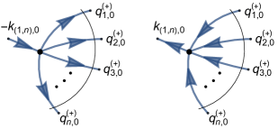
Figure 1: Graphical interpretation of the causal configurations encoded by $\lambda^{-}_{(1,n)}$ (right). If the total external momentum is outgoing, $k_{(1,n),0}>0$, a threshold singularity arises when all the internal momenta are on shell and their three-momenta flow towards the interaction vertex. The mirror configuration encoded by $\lambda^{+}_{(1,n)}$ (left) generates a threshold singularity if $k_{(1,n),0}<0$.

In order to have a deeper understanding of the structures leading to the causal singularities, we can exploit the most relevant features of the LTD formalism. The LTD representation of Eq. (1) is obtained by integrating out one of the components of the loop momenta through the Cauchy’s residue theorem, then reducing the dimensionality of the integration domain by one unit per loop. The integration of the energy component is advantageous because the remaining integration domain, defined by the loop three-momenta, is Euclidean. Nevertheless, the LTD theorem is valid in any coordinate system Catani:2008xa ; Verdugo:2020kzh . As a result, Feynman loop integrals or scattering amplitudes are recast as a sum of nested residues, each term representing a contribution in which $L$ internal particles have been set on shell in such a way that the loop configuration is open to a connected tree. Explicitly, after all the nested residues are summed up, noncausal contributions are analytically cancelled and the loop integral in Eq. (1) takes the causal dual representation

$${\cal A}_{D}^{(L)}=\int_{\vec{\ell}_{1}\ldots\vec{\ell}_{L}}\frac{1}{x_{n}}\sum_{\sigma\in\Sigma}\frac{{\cal N}_{\sigma(i_{1},\ldots,i_{n-L})}}{\lambda_{\sigma(i_{1})}^{\sigma(h_{1})}\cdots\lambda_{\sigma(i_{n-L})}^{\sigma(h_{n-L})}}+(\lambda_{p}^{+}\leftrightarrow\lambda_{p}^{-})~{},$$ (4)

with $x_{n}=\prod_{n}2q_{i,0}^{(+)}$ and $\int_{\vec{\ell}_{s}}=-\mu^{4-d}\int d^{d-1}\ell_{s}/(2\pi)^{d-1}$ the integration measure in the loop three-momentum space. The Feynman propagators from Eq. (1) are substituted in Eq. (4) by causal propagators of the form $1/\lambda_{p}^{\pm}$, where

$$\lambda_{p}^{\pm}=\sum_{i\in p}q_{i,0}^{(+)}\pm k_{p,0}~{},$$ (5)

where $p$ is a partition of the set of on-shell energies, and $k_{p,0}$ is a linear combination of the energy components of the external momenta. Causal propagators may appear raised to a power if the Feynman propagators in the original representation are raised to a power, for example due to self-energy insertions. Each $\lambda_{p}^{\pm}$ is associated to a kinematic configuration in which the momentum flows of all the propagators that belong to the partition $p$ are aligned in the same direction. A graphical interpretation is provided in Fig. 1. Any other configuration cannot be interpreted as causal and is absent from Eq. (4). Depending on the sign of $k_{p,0}$, either $\lambda_{p}^{+}$ or $\lambda_{p}^{-}$ becomes singular when all the propagators in $p$ are set on shell.

The set $\Sigma$ in Eq. (4) contains all the combinations of causal denominators that are entangled, i.e. whose momentum flows are compatible with each other and therefore represent causal thresholds that can occur simultaneously. Each element in $\Sigma$ fixes the momentum flows of all propagators in specific directions. Conversely, once the momentum flows of all propagators are fixed, the causal representation in Eq. (4) can be bootstrapped. In the next section, we will explain in more details the geometrical concepts that justify these results, establishing a connection with the formalism presented in Refs. TorresBobadilla:2021ivx ; Sborlini:2021owe .

The LTD causal representation has similarities with Cutkosky’s rules Cutkosky:1960sp and Steinmann’s relations steinmann ; Stapp:1971hh ; Cahill:1973qp ; Caron-Huot:2016owq ; Caron-Huot:2019bsq ; Benincasa:2020aoj ; Bourjaily:2020wvq ; TorresBobadilla:2021ivx in that it only exhibits the physical or causal singularities but it is essentially different in that it provides the full integral, and not solely the associated discontinuities.

3 Geometric interpretation of causal flows

Originated from the perturbative expansion of the path integral, multiloop scattering amplitudes are described by Feynman diagrams made of vertices and lines connecting them. Whilst vertices codify interactions among particles, lines are associated to virtual states propagating before/after the interactions take place. These Feynman diagrams might contain closed paths or loops, which symbolise quantum fluctuations involving the emission and subsequent absorption of a virtual particle. As described in the previous section, the number of loops corresponds to the number of free integration variables in Eq. (1).

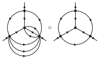
Figure 2: Causal equivalence of a multiloop Feynman diagram (left) with a reduced Feynman graph made of edges obtained by merging all propagators connecting a pair of vertices (right).

However, the dual causal representations presented in Refs. Verdugo:2020kzh ; Aguilera-Verdugo:2020kzc ; Ramirez-Uribe:2020hes can be described by relying on reduced Feynman graphs built from vertices and edges TorresBobadilla:2021ivx ; Sborlini:2021owe . Considering a number of propagators (lines) connecting a pair of interaction vertices, the only possible causal configurations are those in which the momentum flow of all the propagators are aligned in the same direction. As a result, and with the purpose of bootstrapping the causal configurations, a multiloop bunch of propagators can be replaced by a single edge representing the common momentum flow TorresBobadilla:2021ivx ; Sborlini:2021owe , see Fig. 2. This replacement is further supported by the explicit demonstrations reported in Ref. Aguilera-Verdugo:2020nrp .

Once propagators have been collapsed into edges, we can count the number of actual loops in the reduced Feynman graph: these are the so-called eloops. We would like to emphasize that the number of eloops is always smaller (or equal) to the number of loops. Whilst the latter counts the number of primitive integration variables, the former refers to a purely graphical and topological property of the reduced Feynman graph.

Following the geometrical description of Feynman diagrams, we introduce a topological classification related to the number of vertices, $V$. In concrete, we define the order of a reduced diagram as $k=V-1$, which corresponds to the number of off-shell lines involved in the dual representation. In fact, it can be shown that $k=n-L$, and thus the order of the diagram coincides with the number of causal propagators that are being multiplied in each term of the causal representation in Eq. (4).

At this point, let us comment on the reconstruction of the causal structure and some of the available computational strategies for that purpose. Causal propagators, $1/\lambda_{p}^{\pm}$, are identified efficiently starting from the connected binary partitions of vertices of the reduced Feynman graph. Once the causal propagators are known, the representation in Eq. (4) can be recovered by identifying all the possible causal compatible combinations of $k$ causal propagators: these are the so-called causal entangled thresholds. There are three conditions that determine the allowed entanglements Sborlini:2021owe :

1. The combination of $k$ causal propagators depends on the on-shell energies of all the edges.

2. The two sets of vertices associated to two causal propagators are disjoint, or one of them is totally included in the other. For instance, if a maximally connected graph (i.e. a graph where all the vertices are connected to each other) is composed by the vertices $V=\{1,2,3,4,5\}$, then $\lambda_{1}=\{2,3,4\}$ and $\lambda_{2}=\{1,3,4\}$ cannot be simultaneously entangled since their intersection is not empty. But, $\lambda_{1}$ and $\lambda_{3}=\{2,3\}$ are causal-compatible because $\{2,3\}\subset\{2,3,4\}$.

3. Causal flow: The momentum of the edges that crosses a given binary partition of vertices (i.e. each $\lambda_{i}$ being entangled) must be consistently aligned. Momentum must flow from one partition to a different one.

The strategy to successfully identify the set $\Sigma$ in Eq. (4) consists in following the conditions 1 to 3, in that specific order, as already implemented in Refs. Sborlini:2021owe ; Sborlini:2021nqu . Remarkably, the third condition can be reinterpreted as the directed graphs associated to the reduced Feynman diagram. Since momenta must exit one partition and enter into a different one, there cannot be closed cycles. This means that condition 3 is equivalent to identifying all possible directed acyclic graphs compatible with a given set of causal propagators $\{\lambda_{i_{1}}^{h_{1}},\ldots,\lambda_{i_{k}}^{h_{k}}\}$. In this way, another reformulation exists for the causal reconstruction:

1. Causal flow: Identify all the possible directed acyclic graphs obtained from the original reduced Feynman graph.

2. Dress each causal configuration with all the possible combinations of entangled causal propagators fulfilling conditions 1-2 of the previous listing.

Both approaches turn out to be equivalent, and this justifies our focus on the detection of causal configurations from the corresponding directed acyclic graphs. However, the identification of directed acyclic graphs is known to be very time-demanding in classical computations (as will be later exposed in Sec. 5.5). This motivates the search for alternatives that could provide any possible speed-up. In the following we will explain how to use quantum algorithms for such a purpose. This can be considered as a first step towards a fully quantum approach to the identification of entangled causal thresholds.

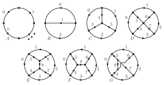
Figure 3: Representative multiloop topologies with up to four eloops. The direction of the arrows corresponds to the $|{1}\rangle$ states. The vertices may or may not have attached external momenta. Beyond one eloop, each line can be composed of $n_{i}$ edges that introduce additional vertices. From left to right and top to bottom: one eloop with $n$ vertices, two eloops (MLT), three eloops (N²MLT), four eloops with one four-particle vertex (N³MLT), and four eloops with trivalent interactions (N⁴MLT), $t$-, $s$- and $u$-channels.

In Fig. 3, we show the representative multiloop topologies that we have considered in this work. We follow the classification scheme introduced in Refs. Aguilera-Verdugo:2020kzc ; Ramirez-Uribe:2020hes , where loop diagrams are ranked according to the number of sets of propagators that depend on different linear combinations of the loop momenta, starting from the maximal loop topology (MLT) with $L+1$ sets, to N^kMLT with $L+1+k$ sets. An extended classification has been introduced in Ref. TorresBobadilla:2021ivx that considers all the vertices connected to each other.

4 Quantum algorithm for causal querying

Following the standard Grover’s querying algorithm Grover:1997fa over unstructured databases, we start from a uniform superposition of $N=2^{n}$ states

$$|{q}\rangle=\frac{1}{\sqrt{N}}\sum_{x=0}^{N-1}|{x}\rangle~{},$$ (6)

which can also be seen as the superposition of one winning state $|{w}\rangle$, encoding all the causal solutions in a uniform superposition, and the orthogonal state $|{q_{\perp}}\rangle$, that collects the noncausal states

$$|{q}\rangle=\cos\theta\,|{q_{\perp}}\rangle+\sin\theta\,|{w}\rangle~{}.$$ (7)

The mixing angle is given by $\theta=\arcsin\sqrt{r/N}$, where $r$ is the number of causal solutions, and the winning and orthogonal uniform superpositions are given by

$$|{w}\rangle=\frac{1}{\sqrt{r}}\sum_{x\in w}|{x}\rangle~{},\qquad|{q_{\perp}}\rangle=\frac{1}{\sqrt{N-r}}\sum_{x\notin w}|{x}\rangle~{}.$$ (8)

The algorithm requires two operators, the oracle operator

$$U_{w}=\boldsymbol{I}-2|{w}\rangle\langle{w}|~{},$$ (9)

that flips the state $|{x}\rangle$ if $x\in w$, $U_{w}|{x}\rangle=-|{x}\rangle$, and leaves it unchanged otherwise, $U_{w}|{x}\rangle=|{x}\rangle$ if $x\notin w$, and the Grover’s diffusion operator

$$U_{q}=2|{q}\rangle\langle{q}|-\boldsymbol{I}~{},$$ (10)

that performs a reflection around the initial state $|{q}\rangle$. The iterative application of both operators $t$ times leads to

$$(U_{q}U_{w})^{t}|{q}\rangle=\cos\theta_{t}\,|{q_{\perp}}\rangle+\sin\theta_{t}\,|{w}\rangle~{},$$ (11)

where $\theta_{t}=(2t+1)\,\theta$. The goal is then to reach a final state such that the probability of each of the components in the orthogonal state is much smaller than the probability of each of the causal solutions by choosing $\theta_{t}$ accordingly:

$$\frac{\cos^{2}\theta_{t}}{N-r}\ll\frac{\sin^{2}\theta_{t}}{r}~{}.$$ (12)

This goal is achieved when $\sin^{2}\theta_{t}\sim 1$.

Grover’s standard algorithm works well if $\theta\leq\pi/6$, namely $r\leq N/4$, but does not provide the desired amplitude amplification of the winning states for larger angles. For example, if $\theta=\pi/3$ the first iteration leads to $\theta_{1}=\pi$ which in fact suppresses the projection onto the set of solutions, while for $\theta=\pi/4$ or $r=N/2$ no matter how many iterations are enforced the probabilities of the initial states remain unchanged. One of the strategies that we apply, which is also valid for other problems where the number of solutions is larger than $N/4$, is to enlarge the total number of states without increasing the number of solutions by introducing ancillary qubits in the register that encodes the edges of the loop diagram . In general, the maximum number of ancillary qubits needed is two, as this increases the number of total states by a factor of $4$. Furthermore, for Feynman loop diagrams we will take advantage of the fact that given a causal solution (directed acyclic configuration), the mirror state in which all internal momentum flows are reversed is also a causal solution. Therefore, we will single out one of the edges and consider that only one of its states contributes to the winning set, while the mirror states are directly deduced from the selected causal solutions. As a result, the complete set of causal solutions can be determined with the help of at most one ancillary qubit.

Three registers are needed for the implementation of the quantum algorithm, together with another qubit that is used as marker by the Grover’s oracle. The first register, whose qubits are labelled $q_{i}$, encode the states of the edges. The qubit $q_{i}$ is in the state $|{1}\rangle$ if the momentum flow of the corresponding edge is oriented in the direction of the initial assignment and in $|{0}\rangle$ if it is in the opposite direction (see Fig. 3). In any case, the final physical result is independent of the initial assignment, being used only as a reference.

The second register, named $c_{ij}$, stores the Boolean clauses that probe whether or not two qubits representing two adjacent edges are in the same state (whether or not are oriented in the same direction). These binary clauses are defined as

$$c_{ij}\equiv(q_{i}=q_{j})~{},$$

$$\bar{c}_{ij}\equiv(q_{i}\neq q_{j})~{},\qquad i,j\in\{0,\ldots,n-1\}~{}.$$ (13)

The third register, $a_{k}(\{c_{ij}\},\{\bar{c}_{ij}\})$, encodes the loop clauses that probe if all the qubits (edges) in each of the eloops that are part of the diagram form a cyclic circuit.

The causal quantum algorithm is implemented as follows. The initial uniform superposition is obtained by applying Hadamard gates to each of the qubits in the $q$-register, $|{q}\rangle=H^{\otimes n}|{0}\rangle$, while the qubit which is used as Grover’s marker is initialized to

$$|{out_{0}}\rangle=\frac{|{0}\rangle-|{1}\rangle}{\sqrt{2}}\equiv|{-}\rangle\,,$$ (14)

which corresponds to a Bell state in the basis $\{|{0}\rangle,|{1}\rangle\}$. The other registers, $|{c}\rangle$ and $|{a}\rangle$, used to store the binary and eloop clauses are initialized to $|{0}\rangle$. Each binary clause $\bar{c}_{ij}$ requires two CNOT gates operating between two qubits in the $|{q}\rangle$ register and one qubit in the $|{c}\rangle$ register. An extra XNOT gate acting on the corresponding qubit in $|{c}\rangle$ is needed to implement a $c_{ij}$ binary clause.

The oracle is defined as

$$U_{w}|{q}\rangle|{c}\rangle|{a}\rangle|{out_{0}}\rangle=(-1)^{f(a,q)}\,|{q}\rangle|{c}\rangle|{a}\rangle|{out_{0}}\rangle~{}.$$ (15)

Therefore, if all the causal conditions are satisfied, $f(a,q)=1$, the corresponding states are marked; otherwise, if $f(a,q)=0$, they are left unchanged. After the marking, the $|{c}\rangle$ and $|{a}\rangle$ registers are rotated back to $|{0}\rangle$ by applying the oracle operations in inverse order. Then, the diffuser $U_{q}$ is applied to the register $|{q}\rangle$. We use the diffuser described in the IBM Qiskit website .

eloops (edges per set)	$|{q}\rangle$	$|{c}\rangle$	$|{a}\rangle$	Total
one ($n$)	$n+1$	$n-1$	$1$	$2n+2$
two ($n_{0},n_{1},n_{2}$)	$n$	$n$	$3$	$2n+4$
three ($n_{0},\ldots,n_{5}$)	$n$	$n+(2$ to $3)$	$4$ to $7$	$2n+(7$ to $11)$
four ($n_{0},\ldots,n_{7}$)	$n$	$n+(3$ to $6)$	$5$ to $13$	$2n+(9$ to $20)$
four ($n_{0},\ldots,n_{8}^{(t,s)}$)	$n$	$n+(4$ to $7)$	$5$ to $13$	$2n+(10$ to $21)$
four ($n_{0},\ldots,n_{8}^{(u)}$)	$n$	$n+(5$ to $8)$	$9$ to $13$	$2n+(15$ to $22)$

Table 1: Number of qubits in each of the three main registers. The total number of qubits includes the ancillary qubit which is initialized to $|{-}\rangle$ to implement Grover’s oracle. Measurements are made on $n=\sum n_{i}$ classical bits.

The upper and lower limit in the number of qubits needed to analyze loop topologies of up to four eloops is summarized in Tab. 1. The final number of qubits depends on the internal configuration of the loop diagram. The lower limit is achieved if $n_{i}=1$ for all the sets, the upper limit is saturated for $n_{i}\geq 2$. Specific details on the implementation of the quantum algorithm and causal clauses are provided in the next section. We use two different simulators: IBM Quantum provided by the open source Qiskit framework; and Quantum Testbed (QUTE) alonso_raul_2021_5561050 , a high performance quantum simulator developed and maintained by Fundación Centro Tecnológico de la Información y la Comunicación (CTIC) .

The output of the Grover’s algorithm described above is a quantum state that is predominantly a superposition of the whole set of causal solutions, with a small contribution from orthogonal states. After a measurement, a single configuration is determined and the superposition is lost. If one requires knowing all solutions and not just a single one, the original output of Grover’s algorithm has then to be prepared and measured a certain number of times, also called shots, large enough in order to scan over all causal solutions, and to distinguish them from the less probable noncausal states. The final result is represented by frequency histograms and is affected by the statistical fluctuations that are inherent to the measurements of a quantum system. Our approach is based on Grover’s search algorithm and, as such, has a similar quantum depth compared to the original implementation and thus a well-known noisy performance on a real present device 9151202 ; PhysRevA.102.042609 ; QuantumInfProcess20 . Given the quantum depth of the algorithm and the resulting difficulties in introducing a reliable error mitigation strategy, we will only consider error-free statistical uncertainties in quantum simulators. Nevertheless, for the sake of benchmarking, we will present a simulation on a real device for the less complex multiloop topology we have analyzed.

We estimate that the number of shots required to distinguish causal from noncausal configurations with a statistical significance of $\Delta\sigma$ standard deviations in a quantum simulator is given by

$$N_{\rm shots}\approx r\left(\Delta\sigma\right)^{2}\left(1+{\cal O}(\cos^{2}(\theta_{t}))\right)\,,$$ (16)

assuming that an efficient amplification of the causal states is achieved, i.e. $\cos(\theta_{t})\sim 0$.

For the identification of causal configurations of the multiloop topologies shown in Fig. 3, for which the number of solutions is of the order of $1/4$ of the total number of states, the quantum advantage over classical algorithms is suppressed by the number of required measurements given by Eq. (16). However, as we will explain in Sec. 5.5, the number of states fulfilling causal-compatible conditions for increasingly complex topologies is much smaller than the total combinations of thresholds. Thus, for very complex topologies which are less affordable with a classical computation, we turn back to the original quantum speed-up provided by Grover’s algorithm. In the following, we will consider $\Delta\sigma\gtrsim 3$, which provides a sufficiently safe discriminant yield with a minimal number of shots.

5 Benchmark multiloop topologies

After introducing the quantum algorithm that identifies the causal configurations of multiloop Feynman diagrams in Sec. 4 and explaining the connection between acyclic graphs and causality in Sec. 3, we present here concrete examples. We consider several topological families of up to four eloops, discussing in each case the explicit implementation of the Boolean clauses and explaining the results obtained.

5.1 One eloop

The one-eloop topology consists of $n$ vertices connected with $n$ edges along a one loop circuit (see Fig. 3A). Each vertex has an external particle attached to it, although it is also possible to have vertices without attached external momenta that are the result of collapsing, e.g., a self-energy insertion into a single edge as explained in Sec. 3.

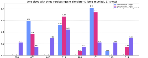
Figure 4: Probability distribution of causal and noncausal configurations obtained with (blue) and without (purple) an ancillary qubit for a one-eloop three-vertex topology. Results are presented with both the IBM quantum simulator and the real quantum device.

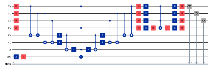
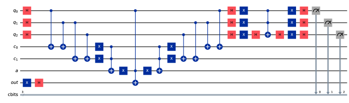
Figure 5: Quantum circuits used to bootstrap the causal configuration of a three-vertex multiloop Feynman diagram. Implementation with (up) and without (down) an ancillary qubit.

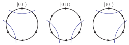
Figure 6: Causal bootstrapping of the one-eloop three-vertex topology. Configurations with all internal momentum flows reversed (not shown) are also causal.

We need to check $n-1$ binary clauses, and there is one Boolean condition that has to be fulfilled

$$a_{0}(\{c_{ij}\})\equiv\neg\left(c_{01}\wedge c_{12}\wedge\cdots\wedge c_{n-2,n-1}\right)~{}.$$ (17)

The qubit $a_{0}$ is set to one if not all the edges are oriented in the same direction. This condition is implemented by imposing a multicontrolled Toffoli gate followed by a Pauli-X gate. We know, however, that this condition is fulfilled for $N-2$ states at one eloop. Therefore, the initial Grover’s angle tends to $\left.\arcsin\left(\sqrt{(N-2)/N}\right)\right|_{n\to\infty}=\pi/2$. In order to achieve the suppression of the orthogonal states, we introduce one ancillary qubit, $q_{n}$, and select one of the states of one of the qubits representing one of the edges. The required Boolean marker is given by

$$f^{(1)}(a,q)=a_{0}\wedge q_{0}\wedge q_{n}~{},$$ (18)

which is also implemented through a multicontrolled Toffoli gate.

The ratio of probabilities of measuring a winning state versus an orthogonal state is enhanced by adding the ancillary qubit. Alternatively, we can still rely on the original Grover’s algorithm when the number of noncausal configurations is small, by swapping the definition of winning and orthogonal states. However, the ancillary qubit is absolutely necessary when the number of winning solutions is ${\cal O}(N/2)$.

The output of the algorithm for a three-vertex multiloop topology is illustrated in Fig. 4, where we extract and compare the selection of causal states with and without the ancillary qubit. The corresponding quantum circuits are represented in Fig. 5. The ancillary qubit is set in superposition with the other qubits but is not measured because this information is irrelevant. Note that in the Qiskit convention qubits are ordered in such a way that the last qubit appears on the left-most side of the register $|{q}\rangle$.

Fig. 6 shows the corresponding directed acyclic configurations and the bootstrapped causal interpretation in terms of causal thresholds. Once the direction of the edges is fixed by the quantum algorithm, the causal thresholds are determined by considering all the possible on-shell cuts with aligned edges that are compatible or entangled with each other. This information can be translated directly into the LTD causal representation in Eq. (4); the on-shell energies $q_{i,0}^{(+)}$ that contribute to a given causal denominator, $\lambda_{p}^{\pm}$, are those related through the same threshold.

The quantum depth of the circuit estimated by Qiskit is $25$ in the simulator, while it amounts to ${\cal O}(200)$ with the ancillary qubit, and ${\cal O}(150)$ without the ancillary qubit in a real device where not all the qubits are connected to each other. The circuit depth is therefore too large to provide a good result in a present real device, as illustrated in Fig. 4. We will focus hereafter on the results obtained by quantum simulators. They are in full agreement with the expectations.

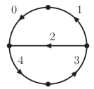
Figure 7: Two-eloop five-edge topology.

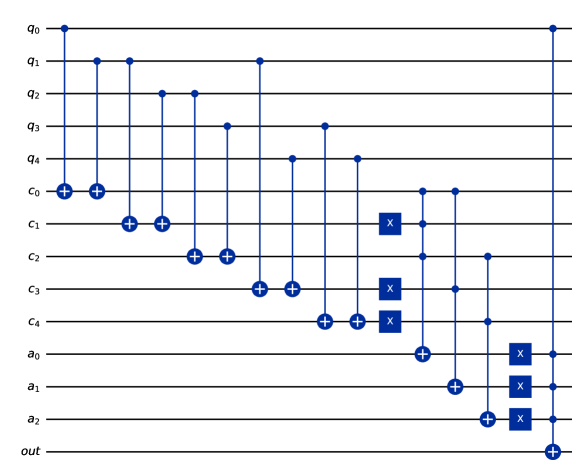
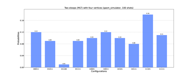
Figure 8: Oracle of the quantum circuit (up, omitting the reflection of the quantum gates) and probability distribution of causal and noncausal configurations (down) for a two-eloop topology (MLT) with $n_{0}=n_{2}=2$ and $n_{1}=1$ edges.

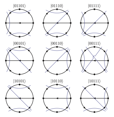
Figure 9: Causal bootstrapping of the two-eloop five-edge topology. Configurations with all internal momentum flows reversed (not shown) are also causal.

5.2 Two eloops

We now analyze multiloop topologies with two eloops (see Fig. 3B). These topologies are characterized by three sets of edges with $n_{0}$, $n_{1}$ and $n_{2}$ edges in each set and two common vertices. The first non-trivial configuration requires that at least two of the sets contain two or more edges. If $n_{0}=n_{1}=n_{2}=1$, we have a multibanana or MLT configuration with $L+1$ propagators which is equivalent to one edge, while the NMLT configuration with $L+2$ sets of propagators, or $n_{0}=2$ and $n_{1}=n_{2}=1$, is equivalent to the one-eloop three-vertex topology already analyzed in Sec. 5.1 because propagators in the sets 1 and 2 can be merged into a single edge. We consider the five-edge topology depicted in Fig. 7 as the first non at two ops. The diagram is composed by three subloops, and therefore requires to test three combinations of binary clauses

$$a_{0}=\neg\left(c_{01}\wedge c_{13}\wedge c_{34}\right)~{},$$

$$a_{1}=\neg\left(c_{01}\wedge\bar{c}_{12}\right)~{},$$

$$a_{2}=\neg\left(c_{23}\wedge c_{34}\right)~{}.$$ (19)

We know from a classical computation Aguilera-Verdugo:2020kzc that the number of causal solutions over the total number of states is $18/32\sim 1/2$. Therefore, it is sufficient to fix the state of one of the edges to reduce the number of states queried to less than $1/4$, while the ancillary $q_{n}$-qubit is not necessary. We select $q_{2}$ as the qubit whose state is fixed, and check the Boolean condition

$$f^{(2)}(a,q)=(a_{0}\wedge a_{1}\wedge a_{2})\wedge q_{2}~{}.$$ (20)

The oracle of the quantum circuit and its output in the IBM’s Qiskit simulator are shown in Fig. 8, and the causal interpretation is provided in Fig. 9. The number of states selected in Fig. 8 is $9$, corresponding to $18$ causal states when considering the mirror configurations obtained by inverting the momentum flows, and in full agreement with the classical calculation.

The generalization to an arbitrary number of edges requires to check first if all the edges in each set are aligned. We define

$$b_{s}=\underset{i_{s}\in s}{\wedge}c_{i_{s},i_{s}+1}~{},\qquad s\in\{0,1,2\}~{}.$$ (21)

The number of subloops is always three, and so the number of conditions that generalize Eq. (19)

$$a_{0}=\neg\left(b_{0}\wedge c_{0_{0}(n_{2}-1)}\wedge b_{2}\right)~{},$$

$$a_{1}=\neg\left(b_{0}\wedge\bar{c}_{(n_{0}-1)(n_{1}-1)}\wedge b_{1}\right)~{},$$

$$a_{2}=\neg\left(b_{1}\wedge c_{(n_{1}-1)0_{2}}\wedge b_{2}\right)~{},$$ (22)

where $0_{s}$ represents the first edge of the set $s$, and $(n_{s}-1)$ is the last one. The total number of qubits required to encode these configurations is summarized in Tab. 1. With 32 qubits as the upper limit in the IBM Qiskit simulator, one can consider any two-eloop topology with $\sum n_{i}\leq 14$ distributed in three sets.

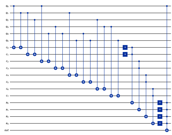
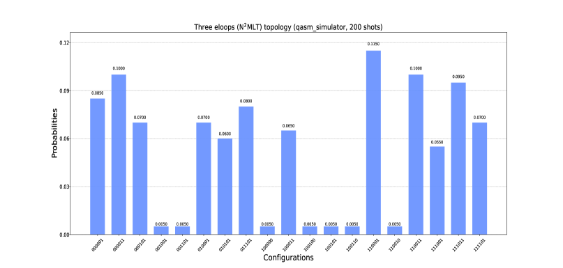
Figure 10: Oracle of the quantum circuit (up, omitting the reflection of the quantum gates) and probability distribution of causal and noncausal configurations (down) for a three-eloop topology (Mercedes topology or N²MLT with $n_{i}=1$).

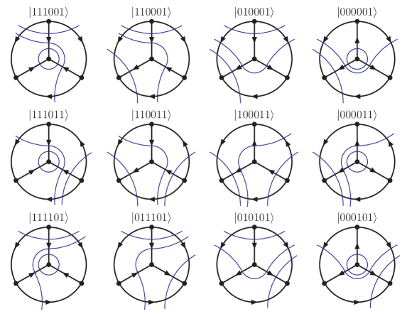
Figure 11: Causal bootstrapping of the three-eloop topology (N²MLT). Configurations with all internal momentum flows reversed (not shown) are also causal.

5.3 Three eloops

The N²MLT multiloop topology (see Fig. 3C) is characterized by four vertices connected through six sets of edges, and $n_{i}$ edges in each set, $i\in\{0,\ldots,5\}$. It appears for the first time at three loops. The algorithm for the multiloop topology with $n_{i}=1$ requires to test the following loop clauses

$$a_{0}=\neg\left(c_{01}\wedge c_{12}\right)~{},$$

$$a_{1}=\neg\left(\bar{c}_{04}\wedge\bar{c}_{34}\right)~{},$$

$$a_{2}=\neg\left(\bar{c}_{15}\wedge\bar{c}_{45}\right)~{},$$

$$a_{3}=\neg\left(\bar{c}_{23}\wedge\bar{c}_{35}\right)~{}.$$ (23)

It is worth noticing that the loop clauses can be implemented in several ways. For example the following expressions are equivalent

$$\left(\bar{c}_{04}\wedge\bar{c}_{34}\right)=\left(c_{03}\wedge\bar{c}_{34}\right)~{}.$$ (24)

However, the expression on the l.h.s. of Eq. (24) requires one NOT gate less than the one on the r.h.s., so it is preferable. It is also worth mentioning that testing loop clauses involving four edges, such as

$$\neg(\bar{c}_{35}\wedge\bar{c}_{15}\wedge c_{01})~{},$$ (25)

is not necessary because four-edge loops enclose one qubit that in any of its states would create a cyclic three-edge loop if the other four edges are oriented in the same direction. The final Boolean condition is

$$f^{(3)}(a,q)=(a_{0}\wedge\ldots\wedge a_{3})\wedge q_{0}~{}.$$ (26)

The oracle of the quantum circuit and probability distribution are shown in Fig. 10, and the causal interpretation is given in Fig. 11. The number of causal configurations is $24$ out of $64$ potential configurations.

For configurations with an arbitrary number of edges the loop clauses in Eq. (23) are substituted by

$$a_{0}=\neg\left(b_{0}\wedge c_{(n_{0}-1)0_{1}}\wedge b_{1}\wedge c_{(n_{1}-1)0_{2}}\wedge b_{2}\right)~{},$$

$$a_{1}=\neg\left(b_{0}\wedge\bar{c}_{(n_{0}-1)(n_{4}-1)}\wedge b_{4}\wedge\bar{c}_{0_{4}0_{3}}\wedge b_{3}\right)~{},$$

$$a_{2}=\neg\left(b_{1}\wedge\bar{c}_{(n_{1}-1)(n_{5}-1)}\wedge b_{5}\wedge\bar{c}_{0_{5}0_{4}}\wedge b_{4}\right)~{},$$

$$a_{3}=\neg\left(b_{2}\wedge\bar{c}_{(n_{2}-1)(n_{3}-1)}\wedge b_{3}\wedge\bar{c}_{0_{3}0_{5}}\wedge b_{5}\right)~{}.$$ (27)

This is the minimal number of loop clauses at three eloops. For three-eloop configurations with several edges in each set an extra binary clause ($c_{(n_{2}-1)0_{0}}$) and up to three loop clauses may be needed to test cycles over four edge sets. These clauses are

$$a_{4}=\neg\left(b_{0}\wedge c_{(n_{0}-1)0_{1}}\wedge b_{1}\wedge\bar{c}_{(n_{1}-1)(n_{5}-1)}\wedge b_{5}\wedge\bar{c}_{0_{3}0_{5}}\wedge b_{3}\right)~{},$$

$$a_{5}=\neg\left(b_{1}\wedge c_{(n_{1}-1)0_{2}}\wedge b_{2}\wedge\bar{c}_{(n_{2}-1)(n_{3}-1)}\wedge b_{3}\wedge\bar{c}_{0_{4}0_{3}}\wedge b_{4}\right)~{},$$

$$a_{6}=\neg\left(b_{2}\wedge c_{(n_{2}-1)0_{0}}\wedge b_{0}\wedge\bar{c}_{(n_{0}-1)(n_{4}-1)}\wedge b_{4}\wedge\bar{c}_{0_{5}0_{4}}\wedge b_{5}\right)~{}.$$ (28)

The number of qubits reaches the upper limit reflected in Tab. 1 for $n_{i}\geq 2$.

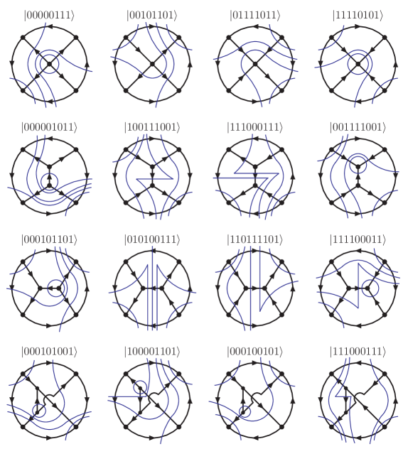
Figure 12: Representative bootstrapped diagrams at four eloops, from the quantum algorithm output in Fig. 14.

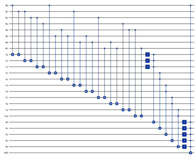
(a) N³MLT

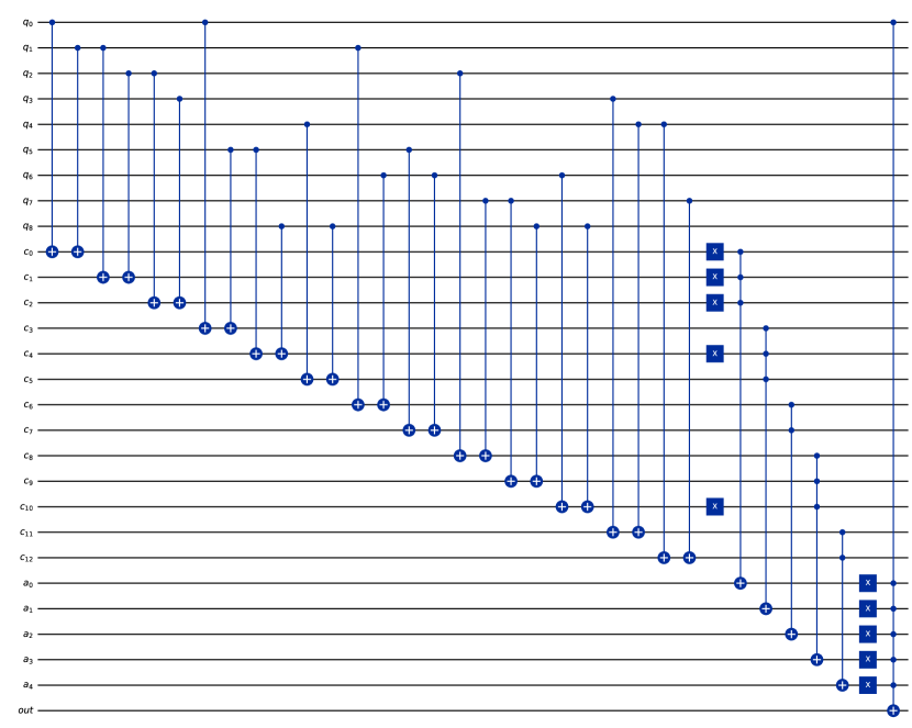
(b) $t$-channel

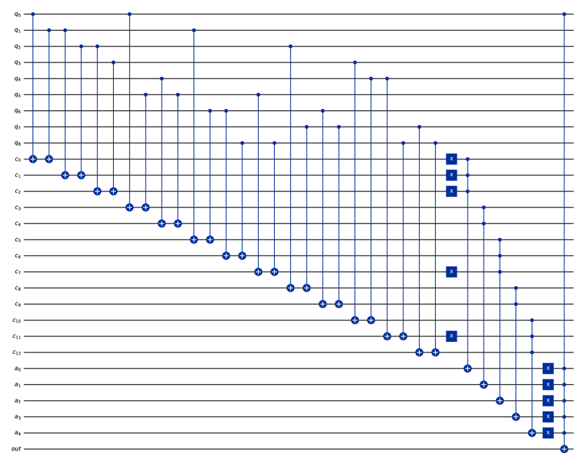
(c) $s$-channel

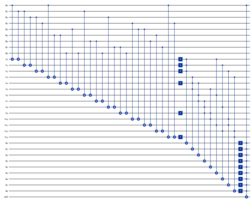
(d) $u$-channel

Figure 13: Oracles of the quantum circuits for four-eloop topologies (omitting the reflection of the quantum gates). (a) N³MLT, (b) $t$-channel, (c) $s$-channels and (d) $u$-channel of N⁴MLT.

5.4 Four eloops

Starting at four loops, we should consider four different topologies (see Fig. 3D to 3G). The N³MLT multiloop topology is characterized by 8 sets of edges connected through $5$ vertices. For $n_{i}=1$, with $i\in\{0,\ldots,7\}$, the loop clauses are

$$a_{0}^{(4)}=\neg\left(c_{01}\wedge c_{12}\wedge c_{23}\right)~{},$$

$$a_{1}^{(4)}=\neg\left(\bar{c}_{05}\wedge\bar{c}_{45}\right)~{},$$

$$a_{2}^{(4)}=\neg\left(\bar{c}_{16}\wedge\bar{c}_{56}\right)~{},$$

$$a_{3}^{(4)}=\neg\left(\bar{c}_{27}\wedge\bar{c}_{67}\right)~{},$$

$$a_{4}^{(4)}=\neg\left(\bar{c}_{34}\wedge\bar{c}_{47}\right)~{},$$ (29)

and the Boolean test function is

$$f^{(4)}(a,q)=(a_{0}^{(4)}\wedge\ldots\wedge a_{4}^{(4)})\wedge q_{0}~{}.$$ (30)

Some of the loop clauses in Eq. (29) are common to the $t$-, $s$- and $u$-channels, which are inclusively denoted as N⁴MLT as they involve each one extra set of edges with respect to N³MLT. The channel specific loop clauses that are needed are

$$a_{1}^{(t)}=\neg\left(\bar{c}_{05}\wedge c_{58}\wedge\bar{c}_{48}\right)~{},\qquad a_{3}^{(t)}=\neg\left(\bar{c}_{27}\wedge\bar{c}_{78}\wedge c_{68}\right)~{},$$ (31)

$$a_{2}^{(s)}=\neg\left(\bar{c}_{16}\wedge\bar{c}_{68}\wedge c_{58}\right)~{},\qquad a_{4}^{(s)}=\neg\left(\bar{c}_{34}\wedge c_{48}\wedge\bar{c}_{78}\right)~{},$$ (32)

and

$$a_{3}^{(u)}=\neg\left(\bar{c}_{27}\wedge c_{78}\wedge\bar{c}_{68}\right)~{},$$

$$a_{4}^{(u)}=\neg\left(\bar{c}_{34}\wedge\bar{c}_{48}\wedge c_{78}\right)~{},$$

$$a_{5}^{(u)}=\neg\left(c_{01}\wedge\bar{c}_{16}\wedge\bar{c}_{46}\right)~{},$$

$$a_{6}^{(u)}=\neg\left(c_{12}\wedge\bar{c}_{27}\wedge\bar{c}_{57}\right)~{},$$

$$a_{7}^{(u)}=\neg\left(c_{23}\wedge\bar{c}_{34}\wedge\bar{c}_{46}\right)~{},$$

$$a_{8}^{(u)}=\neg\left(c_{03}\wedge\bar{c}_{05}\wedge\bar{c}_{57}\right)~{}.$$ (33)

The number of loop clauses for the $u$-channel is much larger than for the other configurations because it is the first nonplanar diagram. Each of the $t$-, $s$- and $u$-channel is characterized by one of the following Boolean conditions

$$f^{(4,t)}(a,q)=\left(a_{0}^{(4)}\wedge a_{1}^{(t)}\wedge a_{2}^{(4)}\wedge a_{3}^{(t)}\wedge a_{4}^{(4)}\right)\wedge q_{0}~{},$$

$$f^{(4,s)}(a,q)=\left(a_{0}^{(4)}\wedge a_{1}^{(4)}\wedge a_{2}^{(s)}\wedge a_{3}^{(4)}\wedge a_{4}^{(s)}\right)\wedge q_{0}~{},$$

$$f^{(4,u)}(a,q)=\left(a_{0}^{(4)}\wedge a_{1}^{(t)}\wedge a_{2}^{(s)}\wedge a_{3}^{(u)}\wedge\ldots\wedge a_{8}^{(u)}\right)\wedge q_{0}~{}.$$ (34)

The number of qubits required for each configuration is given by the lower ranges of Tab. 1, i.e. $25$, $28$, $28$ and $33$ qubits respectively. Despite the complexity of these topologies, the quantum algorithm is well supported by the capacity of the IBM Quantum simulator (see Fig. 14), with the exception of the $u$-channel that was tested within the QUTE Testbed framework as it supports more than 32 qubits (see Fig. 15). Following the procedure described for three-eloop topologies, more complex topologies with $n_{i}\geq 1$ are also amenable to the quantum algorithm, although they may soon exceed the current capacity of the quantum simulator. Representative bootstrapped diagrams at four eloops are shown in Fig. 12. The corresponding oracles of the quantum circuits are presented in Fig. 13.

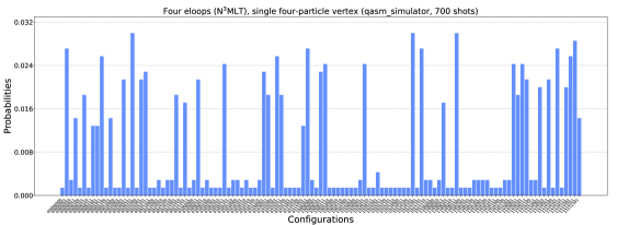
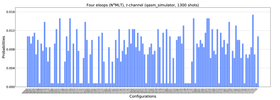
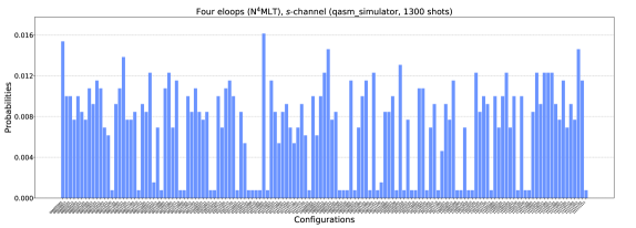
Figure 14: Probability distribution of causal and noncausal configurations for four-eloop topologies after 700, 1300 and 1300 shots with qasm_simulator, respectively in the IBM’s Qiskit framework. From top to down: N³MLT, $t$-, and $s$-channels of N⁴MLT with $n_{i}=1$. The number of selected states is $39/256$, $102/512$ and $102/512$, respectively.

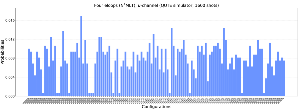
Figure 15: Probability distribution of causal and noncausal configurations for the four-eloop $u$-channel after 1600 shots in the QUTE Testbed framework. The number of selected states is $115/512$.

5.5 Counting of causal states

After discussing the causal structure of multiloop Feynman diagrams, it is clear that detecting all the configurations with causal-compatible momenta flow is crucial to identify the terms involved in the LTD representation of Eq. (4). Also, as explained in Sec. 4, the performance of quantum search algorithms depends on the number of winning states compared to all the possible configurations of the system. Thus, in this section, we present a counting of states fulfilling causality conditions for different topologies.

Given a reduced Feynman graph made of $V$ vertices connected through $n$ edges, there are $N=2^{n}$ possible orientations of the internal edges but only some of them are compatible with causality. Since causal-compatible momentum flows are in a one-to-one correspondence with the number of directed acyclic graphs, $n_{A}$, built from the original reduced Feynman graph, we are interested in estimating the ratio $r_{A}=n_{A}/2^{n}$. In order to do so, let us consider two extreme topologies:

• Maximally Connected Graph (MCG) where all the vertices are connected to each other and $n=V(V-1)/2$.

• Minimally Connected Graph (mCG) with $n=V$, i.e. the minimal number of edges. It only occurs at one eloop.

For a fixed number of vertices $V$, the number of causal-compatible orientations is minimal for MCG and maximal for mCG; the bigger the number of edges, the larger the set of constraints that a graph must fulfil to be free of cycles. In fact, it is easy to show that

$${V!}\leq n_{A}\leq 2^{(V-1)V/2}-2\,,$$ (35)

which implies that, in the limit $V\to\infty$, we have $r_{A}\to 0$ for highly-connected topologies. In other words, for diagrams with a high number of eloops, the ratio $r_{A}$ is generally small. On the other hand, for one eloop diagrams, $r_{A}\to 1$ as $V\to\infty$, which means that the ratio of noncausal flow configurations is small compared to the total number of configurations. In Tab. 2 we present explicit values for the topologies described in Fig. 3, focusing on the number of causal configurations ($n_{A}$).

Diagram	Vertices/Edges	$n_{\lambda}$	$n_{A}/2^{n}$
one eloop ($n=3$)	3/3	3	6/8
two eloops ($n_{0}=n_{2}=2,n_{1}=1$)	4/5	6	18/32
three eloops ($n_{i}=1$)	4/6	7	24/64
N3MLT ($n_{i}=1$)	5/8	13	78/256
N4MLT $t$-channel ($n_{i}=1$)	6/9	22	204/512
N4MLT $s$-channel ($n_{i}=1$)	6/9	22	204/512
N4MLT $u$-channel ($n_{i}=1$)	6/9	24	230/512

Table 2: Number of causal propagators ($n_{\lambda}$) and causal or acyclic configurations ($n_{A}$) for the topologies drawn in Figs. 3 and 9.

With these results on sight, we notice that $n_{A}$ turns out to become a small fraction of the total number of flux-orientation for increasingly complex diagrams. Thus, we expect that the quantum search algorithms perform better against classical algorithms, since the number of winning states is a tiny fraction of the total space of states. On the other hand, when the number of noncausal configurations is small compared with the total number of states, we can revert the definition of Grover’s marker and look for cyclic graphs (i.e. noncausal flow configurations). For instance, for one-eloop topologies, we find that the ratio of noncausal versus total configurations is given by $2^{1-V(V-1)/2}$ and the original version of Grover’s algorithm perfectly applies to this problem.

6 Conclusions

We have presented the first proof-of-concept application of a quantum algorithm to multiloop Feynman integrals exploiting the loop-tree duality and causality. The specific problem we have addressed is the identification of all the causal singular configurations of the loop integrand resulting from setting on shell internal Feynman propagators. This information is useful both for identifying the physical discontinuities of the Feynman loop integral and to bootstrap its causal representation in the loop-tree duality. Beyond particle physics, this is also a challenging problem of identifying directed acyclic graphs.

We have described the quantum algorithm in general terms, and have provided the particular details on its implementation to selected multiloop topologies. These cases were successfully handled by IBM Quantum and QUTE simulators. Even if for these selected topologies the quantum speed-up is attenuated by the number of shots required to identify all the causal configurations, more involved topologies and the selection of configurations satisfying further causality conditions would fully benefit from Grover’s quadratic speed-up.

Given the quantum depth of the algorithm, its execution in current real devices leads to unreliable results due to the present hardware limitations. However, the quantum simulators successfully identifies all causal states even for the most complex multiloop configurations considered.

References

- (1) R. P. Feynman, Simulating physics with computers, Int. J. Theor. Phys. 21 (1982) 467–488.
- (2) L. K. Grover, Quantum mechanics helps in searching for a needle in a haystack, Phys. Rev. Lett. 79 (1997) 325–328, [quant-ph/9706033].
- (3) P. W. Shor, Polynomial time algorithms for prime factorization and discrete logarithms on a quantum computer, SIAM J. Sci. Statist. Comput. 26 (1997) 1484, [quant-ph/9508027].
- (4) B. Apolloni, C. Carvalho and D. de Falco, Quantum stochastic optimization, Stochastic Processes and their Applications 33 (1989) 233–244.
- (5) T. Kadowaki and H. Nishimori, Quantum annealing in the transverse ising model, Phys. Rev. E 58 (Nov, 1998) 5355–5363.
- (6) J. Liu and Y. Xin, Quantum simulation of quantum field theories as quantum chemistry, JHEP 12 (2020) 011, [2004.13234].
- (7) J. E. Lynn, I. Tews, S. Gandolfi and A. Lovato, Quantum Monte Carlo Methods in Nuclear Physics: Recent Advances, Ann. Rev. Nucl. Part. Sci. 69 (2019) 279–305, [1901.04868].
- (8) E. T. Holland, K. A. Wendt, K. Kravvaris, X. Wu, W. Erich Ormand, J. L. DuBois et al., Optimal Control for the Quantum Simulation of Nuclear Dynamics, Phys. Rev. A 101 (2020) 062307, [1908.08222].
- (9) R. Orus, S. Mugel and E. Lizaso, Quantum computing for finance: Overview and prospects, Reviews in Physics 4 (Nov, 2019) 100028.
- (10) R. K. Ellis et al., Physics Briefing Book: Input for the European Strategy for Particle Physics Update 2020, 1910.11775.
- (11) F. Gianotti et al., Physics potential and experimental challenges of the LHC luminosity upgrade, Eur. Phys. J. C 39 (2005) 293–333, [hep-ph/0204087].
- (12) FCC collaboration, A. Abada et al., FCC Physics Opportunities: Future Circular Collider Conceptual Design Report Volume 1, Eur. Phys. J. C 79 (2019) 474.
- (13) ILC collaboration, G. Aarons et al., International Linear Collider Reference Design Report Volume 2: Physics at the ILC, 0709.1893.
- (14) CLIC, CLICdp collaboration, P. Roloff, R. Franceschini, U. Schnoor and A. Wulzer, The Compact Linear e+e- Collider (CLIC): Physics Potential, 1812.07986.
- (15) CEPC Study Group collaboration, M. Dong et al., CEPC Conceptual Design Report: Volume 2 - Physics & Detector, 1811.10545.
- (16) A. Y. Wei, P. Naik, A. W. Harrow and J. Thaler, Quantum Algorithms for Jet Clustering, Phys. Rev. D 101 (2020) 094015, [1908.08949].
- (17) D. Pires, P. Bargassa, J. Seixas and Y. Omar, A Digital Quantum Algorithm for Jet Clustering in High-Energy Physics, 2101.05618.
- (18) D. Pires, Y. Omar and J. Seixas, Adiabatic Quantum Algorithm for Multijet Clustering in High Energy Physics, 2012.14514.
- (19) J. a. Barata and C. A. Salgado, A quantum strategy to compute the jet quenching parameter , Eur. Phys. J. C 81 (2021) 862, [2104.04661].
- (20) A. Pérez-Salinas, J. Cruz-Martinez, A. A. Alhajri and S. Carrazza, Determining the proton content with a quantum computer, Phys. Rev. D 103 (2021) 034027, [2011.13934].
- (21) C. W. Bauer, W. A. de Jong, B. Nachman and D. Provasoli, Quantum Algorithm for High Energy Physics Simulations, Phys. Rev. Lett. 126 (2021) 062001, [1904.03196].
- (22) C. W. Bauer, M. Freytsis and B. Nachman, Simulating Collider Physics on Quantum Computers Using Effective Field Theories, Phys. Rev. Lett. 127 (2021) 212001, [2102.05044].
- (23) W. A. De Jong, M. Metcalf, J. Mulligan, M. Płoskoń, F. Ringer and X. Yao, Quantum simulation of open quantum systems in heavy-ion collisions, Phys. Rev. D 104 (2021) 051501, [2010.03571].
- (24) W. Guan, G. Perdue, A. Pesah, M. Schuld, K. Terashi, S. Vallecorsa et al., Quantum Machine Learning in High Energy Physics, 2005.08582.
- (25) S. L. Wu et al., Application of quantum machine learning using the quantum variational classifier method to high energy physics analysis at the LHC on IBM quantum computer simulator and hardware with 10 qubits, J. Phys. G 48 (2021) 125003, [2012.11560].
- (26) T. Felser, M. Trenti, L. Sestini, A. Gianelle, D. Zuliani, D. Lucchesi et al., Quantum-inspired machine learning on high-energy physics data, npj Quantum Inf. 7 (2021) 111, [2004.13747].
- (27) S. P. Jordan, K. S. M. Lee and J. Preskill, Quantum Algorithms for Quantum Field Theories, Science 336 (2012) 1130–1133, [1111.3633].
- (28) M. C. Bañuls et al., Simulating Lattice Gauge Theories within Quantum Technologies, Eur. Phys. J. D 74 (2020) 165, [1911.00003].
- (29) E. Zohar, J. I. Cirac and B. Reznik, Quantum Simulations of Lattice Gauge Theories using Ultracold Atoms in Optical Lattices, Rept. Prog. Phys. 79 (2016) 014401, [1503.02312].
- (30) T. Byrnes and Y. Yamamoto, Simulating lattice gauge theories on a quantum computer, Phys. Rev. A 73 (2006) 022328, [quant-ph/0510027].
- (31) R. R. Ferguson, L. Dellantonio, K. Jansen, A. A. Balushi, W. Dür and C. A. Muschik, Measurement-Based Variational Quantum Eigensolver, Phys. Rev. Lett. 126 (2021) 220501, [2010.13940].
- (32) A. Kan, L. Funcke, S. Kühn, L. Dellantonio, J. Zhang, J. F. Haase et al., Investigating a (3+1)D topological -term in the Hamiltonian formulation of lattice gauge theories for quantum and classical simulations, Phys. Rev. D 104 (2021) 034504, [2105.06019].
- (33) G. Heinrich, Collider Physics at the Precision Frontier, Phys. Rept. 922 (2021) 1–69, [2009.00516].
- (34) T. Binoth and G. Heinrich, An automatized algorithm to compute infrared divergent multiloop integrals, Nucl. Phys. B 585 (2000) 741–759, [hep-ph/0004013].
- (35) A. Smirnov and M. Tentyukov, Feynman Integral Evaluation by a Sector decomposiTion Approach (FIESTA), Comput. Phys. Commun. 180 (2009) 735–746, [0807.4129].
- (36) J. Carter and G. Heinrich, SecDec: A general program for sector decomposition, Comput. Phys. Commun. 182 (2011) 1566–1581, [1011.5493].
- (37) S. Borowka, G. Heinrich, S. Jahn, S. Jones, M. Kerner, J. Schlenk et al., pySecDec: a toolbox for the numerical evaluation of multi-scale integrals, Comput. Phys. Commun. 222 (2018) 313–326, [1703.09692].
- (38) J. Blumlein, Analytic continuation of Mellin transforms up to two loop order, Comput. Phys. Commun. 133 (2000) 76–104, [hep-ph/0003100].
- (39) C. Anastasiou and A. Daleo, Numerical evaluation of loop integrals, JHEP 10 (2006) 031, [hep-ph/0511176].
- (40) I. Bierenbaum, J. Blumlein and S. Klein, Evaluating Two-Loop massive Operator Matrix Elements with Mellin-Barnes Integrals, Nucl. Phys. B Proc. Suppl. 160 (2006) 85–90, [hep-ph/0607300].
- (41) J. Gluza, K. Kajda and T. Riemann, AMBRE: A Mathematica package for the construction of Mellin-Barnes representations for Feynman integrals, Comput. Phys. Commun. 177 (2007) 879–893, [0704.2423].
- (42) A. Freitas and Y.-C. Huang, On the Numerical Evaluation of Loop Integrals With Mellin-Barnes Representations, JHEP 04 (2010) 074, [1001.3243].
- (43) I. Dubovyk, J. Gluza, T. Riemann and J. Usovitsch, Numerical integration of massive two-loop Mellin-Barnes integrals in Minkowskian regions, PoS LL2016 (2016) 034, [1607.07538].
- (44) P. Mastrolia and G. Ossola, On the Integrand-Reduction Method for Two-Loop Scattering Amplitudes, JHEP 11 (2011) 014, [1107.6041].
- (45) S. Badger, H. Frellesvig and Y. Zhang, Hepta-Cuts of Two-Loop Scattering Amplitudes, JHEP 1204 (2012) 055, [1202.2019].
- (46) Y. Zhang, Integrand-Level Reduction of Loop Amplitudes by Computational Algebraic Geometry Methods, JHEP 09 (2012) 042, [1205.5707].
- (47) P. Mastrolia, E. Mirabella, G. Ossola and T. Peraro, Scattering Amplitudes from Multivariate Polynomial Division, Phys. Lett. B718 (2012) 173–177, [1205.7087].
- (48) P. Mastrolia, E. Mirabella, G. Ossola and T. Peraro, Integrand-Reduction for Two-Loop Scattering Amplitudes through Multivariate Polynomial Division, Phys. Rev. D87 (2013) 085026, [1209.4319].
- (49) H. Ita, Two-loop Integrand Decomposition into Master Integrals and Surface Terms, 1510.05626.
- (50) P. Mastrolia, T. Peraro and A. Primo, Adaptive Integrand Decomposition in parallel and orthogonal space, JHEP 08 (2016) 164, [1605.03157].
- (51) G. Ossola, C. G. Papadopoulos and R. Pittau, Reducing full one-loop amplitudes to scalar integrals at the integrand level, Nucl. Phys. B763 (2007) 147–169, [hep-ph/0609007].
- (52) K. G. Chetyrkin and F. V. Tkachov, Integration by Parts: The Algorithm to Calculate beta Functions in 4 Loops, Nucl. Phys. B192 (1981) 159–204.
- (53) S. Laporta, High precision calculation of multiloop Feynman integrals by difference equations, Int. J. Mod. Phys. A15 (2000) 5087–5159, [hep-ph/0102033].
- (54) F. Moriello, Generalised power series expansions for the elliptic planar families of Higgs + jet production at two loops, JHEP 01 (2020) 150, [1907.13234].
- (55) R. Bonciani, V. Del Duca, H. Frellesvig, J. Henn, M. Hidding, L. Maestri et al., Evaluating a family of two-loop non-planar master integrals for Higgs + jet production with full heavy-quark mass dependence, JHEP 01 (2020) 132, [1907.13156].
- (56) M. Czakon, Tops from Light Quarks: Full Mass Dependence at Two-Loops in QCD, Phys. Lett. B 664 (2008) 307–314, [0803.1400].
- (57) C. Gnendiger et al., To , or not to : recent developments and comparisons of regularization schemes, Eur. Phys. J. C 77 (2017) 471, [1705.01827].
- (58) W. J. Torres Bobadilla et al., May the four be with you: Novel IR-subtraction methods to tackle NNLO calculations, Eur. Phys. J. C 81 (2021) 250, [2012.02567].
- (59) R. Winterhalder, V. Magerya, E. Villa, S. P. Jones, M. Kerner, A. Butter et al., Targeting Multi-Loop Integrals with Neural Networks, 2112.09145.
- (60) S. Camarda, L. Cieri and G. Ferrera, Drell–Yan lepton-pair production: qT resummation at N3LL accuracy and fiducial cross sections at N3LO, Phys. Rev. D 104 (2021) L111503, [2103.04974].
- (61) C. Duhr, F. Dulat and B. Mistlberger, Charged current Drell-Yan production at N3LO, JHEP 11 (2020) 143, [2007.13313].
- (62) J. Currie, T. Gehrmann, E. W. N. Glover, A. Huss, J. Niehues and A. Vogt, N3LO corrections to jet production in deep inelastic scattering using the Projection-to-Born method, JHEP 05 (2018) 209, [1803.09973].
- (63) B. Mistlberger, Higgs boson production at hadron colliders at N3LO in QCD, JHEP 05 (2018) 028, [1802.00833].
- (64) F. Dulat, B. Mistlberger and A. Pelloni, Differential Higgs production at N3LO beyond threshold, JHEP 01 (2018) 145, [1710.03016].
- (65) K. Bepari, S. Malik, M. Spannowsky and S. Williams, Towards a Quantum Computing Algorithm for Helicity Amplitudes and Parton Showers, Phys. Rev. D 103 (2021) 076020, [2010.00046].
- (66) G. Brassard and P. Hoyer, An Exact quantum polynomial- time algorithm for Simon’s problem, in 5th Israeli Symposium on Theory of Computing and Systems (ISTCS 97), 4, 1997. quant-ph/9704027.
- (67) L. K. Grover, Quantum computers can search rapidly by using almost any transformation, Phys. Rev. Lett. 80 (1998) 4329–4332, [quant-ph/9712011].
- (68) G. Brassard, P. Hoyer and A. Tapp, Quantum algorithm for the collision problem, quant-ph/9705002.
- (69) L. K. Grover and J. Radhakrishnan, Is partial quantum search of a database any easier?, arXiv e-prints (July, 2004) quant–ph/0407122, [quant-ph/0407122].
- (70) M. Boyer, G. Brassard, P. Hoyer and A. Tapp, Tight bounds on quantum searching, Fortsch. Phys. 46 (1998) 493–506, [quant-ph/9605034].
- (71) C. Squires, S. Magliacane, K. Greenewald, K. D., K. M. and K. Shanmugam, Active structure learning of causal dags via directed clique tree, 2020.
- (72) G. Chiribella, G. M. D’Ariano and P. Perinotti, Theoretical framework for quantum networks, Phys. Rev. A 80 (Aug, 2009) 022339.
- (73) S. Even and G. Even, Graph Algorithms, second edition, vol. 9780521517188. 2011. 10.1017/CBO9781139015165.
- (74) S. Catani, T. Gleisberg, F. Krauss, G. Rodrigo and J.-C. Winter, From loops to trees by-passing Feynman’s theorem, JHEP 09 (2008) 065, [0804.3170].
- (75) I. Bierenbaum, S. Catani, P. Draggiotis and G. Rodrigo, A Tree-Loop Duality Relation at Two Loops and Beyond, JHEP 10 (2010) 073, [1007.0194].
- (76) I. Bierenbaum, S. Buchta, P. Draggiotis, I. Malamos and G. Rodrigo, Tree-Loop Duality Relation beyond simple poles, JHEP 03 (2013) 025, [1211.5048].
- (77) S. Buchta, G. Chachamis, P. Draggiotis, I. Malamos and G. Rodrigo, On the singular behaviour of scattering amplitudes in quantum field theory, JHEP 11 (2014) 014, [1405.7850].
- (78) R. J. Hernandez-Pinto, G. F. R. Sborlini and G. Rodrigo, Towards gauge theories in four dimensions, JHEP 02 (2016) 044, [1506.04617].
- (79) S. Buchta, G. Chachamis, P. Draggiotis and G. Rodrigo, Numerical implementation of the loop-tree duality method, Eur. Phys. J. C 77 (2017) 274, [1510.00187].
- (80) G. F. R. Sborlini, F. Driencourt-Mangin, R. Hernandez-Pinto and G. Rodrigo, Four-dimensional unsubtraction from the loop-tree duality, JHEP 08 (2016) 160, [1604.06699].
- (81) G. F. R. Sborlini, F. Driencourt-Mangin and G. Rodrigo, Four-dimensional unsubtraction with massive particles, JHEP 10 (2016) 162, [1608.01584].
- (82) E. T. Tomboulis, Causality and Unitarity via the Tree-Loop Duality Relation, JHEP 05 (2017) 148, [1701.07052].
- (83) F. Driencourt-Mangin, G. Rodrigo and G. F. R. Sborlini, Universal dual amplitudes and asymptotic expansions for and in four dimensions, Eur. Phys. J. C 78 (2018) 231, [1702.07581].
- (84) J. Llanes Jurado, G. Rodrigo and W. J. Torres Bobadilla, From Jacobi off-shell currents to integral relations, JHEP 12 (2017) 122, [1710.11010].
- (85) F. Driencourt-Mangin, G. Rodrigo, G. F. R. Sborlini and W. J. Torres Bobadilla, Universal four-dimensional representation of at two loops through the Loop-Tree Duality, JHEP 02 (2019) 143, [1901.09853].
- (86) R. Runkel, Z. Szőr, J. P. Vesga and S. Weinzierl, Causality and loop-tree duality at higher loops, Phys. Rev. Lett. 122 (2019) 111603, [1902.02135].
- (87) R. Baumeister, D. Mediger, J. PeVcovnik and S. Weinzierl, Vanishing of certain cuts or residues of loop integrals with higher powers of the propagators, Phys. Rev. D 99 (2019) 096023, [1903.02286].
- (88) J. J. Aguilera-Verdugo, F. Driencourt-Mangin, J. Plenter, S. Ramírez-Uribe, G. Rodrigo, G. F. R. Sborlini et al., Causality, unitarity thresholds, anomalous thresholds and infrared singularities from the loop-tree duality at higher orders, JHEP 12 (2019) 163, [1904.08389].
- (89) R. Runkel, Z. Szőr, J. P. Vesga and S. Weinzierl, Integrands of loop amplitudes within loop-tree duality, Phys. Rev. D 101 (2020) 116014, [1906.02218].
- (90) Z. Capatti, V. Hirschi, D. Kermanschah and B. Ruijl, Loop-Tree Duality for Multiloop Numerical Integration, Phys. Rev. Lett. 123 (2019) 151602, [1906.06138].
- (91) F. Driencourt-Mangin, G. Rodrigo, G. F. R. Sborlini and W. J. Torres Bobadilla, Interplay between the loop-tree duality and helicity amplitudes, Phys. Rev. D 105 (2022) 016012, [1911.11125].
- (92) Z. Capatti, V. Hirschi, D. Kermanschah, A. Pelloni and B. Ruijl, Numerical Loop-Tree Duality: contour deformation and subtraction, JHEP 04 (2020) 096, [1912.09291].
- (93) J. J. Aguilera-Verdugo, F. Driencourt-Mangin, R. J. Hernández-Pinto, J. Plenter, S. Ramirez-Uribe, A. E. Renteria Olivo et al., Open Loop Amplitudes and Causality to All Orders and Powers from the Loop-Tree Duality, Phys. Rev. Lett. 124 (2020) 211602, [2001.03564].
- (94) J. Plenter and G. Rodrigo, Asymptotic expansions through the loop-tree duality, Eur. Phys. J. C 81 (2021) 320, [2005.02119].
- (95) J. J. Aguilera-Verdugo, R. J. Hernandez-Pinto, G. Rodrigo, G. F. R. Sborlini and W. J. Torres Bobadilla, Causal representation of multi-loop Feynman integrands within the loop-tree duality, JHEP 01 (2021) 069, [2006.11217].
- (96) S. Ramírez-Uribe, R. J. Hernández-Pinto, G. Rodrigo, G. F. R. Sborlini and W. J. Torres Bobadilla, Universal opening of four-loop scattering amplitudes to trees, JHEP 04 (2021) 129, [2006.13818].
- (97) J. Aguilera-Verdugo, R. J. Hernández-Pinto, S. Ramírez-Uribe, G. Rodrigo, G. F. R. Sborlini and W. J. Torres Bobadilla, Manifestly Causal Scattering Amplitudes, in Snowmass 2021 - Letter of Intention, August 2020.
- (98) Z. Capatti, V. Hirschi, D. Kermanschah, A. Pelloni and B. Ruijl, Manifestly Causal Loop-Tree Duality, 2009.05509.
- (99) J. Aguilera-Verdugo, R. J. Hernández-Pinto, G. Rodrigo, G. F. R. Sborlini and W. J. Torres Bobadilla, Mathematical properties of nested residues and their application to multi-loop scattering amplitudes, JHEP 02 (2021) 112, [2010.12971].
- (100) R. M. Prisco and F. Tramontano, Dual subtractions, JHEP 06 (2021) 089, [2012.05012].
- (101) W. J. Torres Bobadilla, Loop-tree duality from vertices and edges, JHEP 04 (2021) 183, [2102.05048].
- (102) G. F. R. Sborlini, Geometrical approach to causality in multiloop amplitudes, Phys. Rev. D 104 (2021) 036014, [2102.05062].
- (103) W. J. T. Bobadilla, Lotty – The loop-tree duality automation, Eur. Phys. J. C 81 (2021) 514, [2103.09237].
- (104) J. Aguilera-Verdugo et al., A Stroll through the Loop-Tree Duality, Symmetry 13 (2021) 1029, [2104.14621].
- (105) C. G. Bollini and J. J. Giambiagi, Dimensional Renormalization: The Number of Dimensions as a Regularizing Parameter, Nuovo Cim. B 12 (1972) 20–26.
- (106) G. ’t Hooft and M. J. G. Veltman, Regularization and Renormalization of Gauge Fields, Nucl. Phys. B 44 (1972) 189–213.
- (107) R. E. Cutkosky, Singularities and discontinuities of Feynman amplitudes, J. Math. Phys. 1 (1960) 429–433.
- (108) O. Steinmann, Uber den Zusammenhang Zwischen den Wightmanfunktionen und den Retardierten Kommutatoren, Helv. Phys. Acta 33 (1960) 257.
- (109) H. P. Stapp, Inclusive cross-sections are discontinuities, Phys. Rev. D3 (1971) 3177–3184.
- (110) K. E. Cahill and H. P. Stapp, Optical theorems and Steinmann relations, Annals Phys. 90 (1975) 438.
- (111) S. Caron-Huot, L. J. Dixon, A. McLeod and M. von Hippel, Bootstrapping a Five-Loop Amplitude Using Steinmann Relations, Phys. Rev. Lett. 117 (2016) 241601, [1609.00669].
- (112) S. Caron-Huot, L. J. Dixon, F. Dulat, M. Von Hippel, A. J. McLeod and G. Papathanasiou, The Cosmic Galois Group and Extended Steinmann Relations for Planar SYM Amplitudes, JHEP 09 (2019) 061, [1906.07116].
- (113) P. Benincasa, A. J. McLeod and C. Vergu, Steinmann Relations and the Wavefunction of the Universe, Phys. Rev. D 102 (2020) 125004, [2009.03047].
- (114) J. L. Bourjaily, H. Hannesdottir, A. J. McLeod, M. D. Schwartz and C. Vergu, Sequential Discontinuities of Feynman Integrals and the Monodromy Group, JHEP 01 (2021) 205, [2007.13747].
- (115) G. F. R. Sborlini, Geometry and causality for efficient multiloop representations, in 15th International Symposium on Radiative Corrections: Applications of Quantum Field Theory to Phenomenology and LoopFest XIX: Workshop on Radiative Corrections for the LHC and Future Colliders, September 2021. 2109.07808.
- (116) M. Nielsen and I. Chuang, Quantum computation and quantum information. 2000. 10.2277/0521635039.
- (117) R. Alonso, A. Arias, P. Coca, F. Díez, A. García and L. Meijueiro, Qute: Quantum computing simulation platform, Oct., 2021. 10.5281/zenodo.5561050.
- (118) T. Satoh, Y. Ohkura and R. Van Meter, Subdivided phase oracle for nisq search algorithms, IEEE Transactions on Quantum Engineering 1 (2020) 1–15.
- (119) Y. Wang and P. S. Krstic, Prospect of using grover’s search in the noisy-intermediate-scale quantum-computer era, Phys. Rev. A 102 (Oct, 2020) 042609.
- (120) K. Zhang, P. Rao, K. Yu, H. Lim and V. Korepin, Implementation of efficient quantum search algorithms on nisq computers, Quantum Inf Process 20 (Jul, 2021) .