Classical-Quantum Noise Mitigation for NISQ Hardware

Abstract

In this work, the global white-noise model is proved from first principles. The adherence of NISQ hardware to the global white-noise model is used to perform noise mitigation using CLAssical White-noise Extrapolation (CLAWE).

I Global White-Noise Model

Universal quantum computation involves the encoding of algorithms into sequences of local gates. The noise processes in Noisy Intermediate-Scale Quantum (NISQ) hardware do not exhibit such locality, resulting in qubit crosstalk [1, 2, 3, 4, 5, 6, 7, 8, 9, 10, 11, 12, 13, 14, 15, 16, 17, 18, 19, 20, 21, 22, 23, 24, 25].

This non-locality suggests a global description of the average noise dynamics. The global white-noise model [26, 27, 28, 29] presumes that the noise dynamics associated with entangling operations [30, 31, 32, 33, 34, 35, 36, 37, 38, 39, 40, 41, 42, 43, 44, 45, 46, 47, 48, 49, 50, 51, 52, 53, 54, 55, 56, 57, 58, 59, 60, 61, 62, 63, 64, 65, 66] can be approximated by depolarizing events that span the entire Hilbert space (Figure 1). The global white-noise model is now derived from first principles using quantum channel technology.

I.1 Introduction to Superoperators

Rigorously treating noise dynamics requires a density matrix representation [67, 68, 69], because the evolution of open quantum systems generates mixed quantum states. Vector representations cannot describe such processes, as they only characterize pure quantum states: $\Ket{\psi}$.

Mixed quantum states have interacted with unknown degrees of freedom. They are composed of an ensemble of pure states $\{\Ket{\psi_{k}}\}$, with observational probabilities $\{\alpha_{k}\}$. The corresponding density matrix is the following:

$$\rho_{\text{\tiny mixed}}=\sum_{k}\alpha_{k}\Ket{\psi_{k}}\kern-1.49994pt\bra{\psi_{k}}$$ (I.1)

In the density matrix representation, $d\kern-1.34995pt\times\kern-1.34995ptd$-dimensional operators that act on wavefunctions, generalize to $d^{2}\kern-1.34995pt\times\kern-1.34995ptd^{2}$-dimensional quantum channels known as superoperators. Each superoperator can be represented by sets of Kraus operators {$M_{k}$} [70]:

$$\hat{\mathcal{E}}=\sum^{\mathcal{R}}_{k=1}M_{k}\otimes M_{k}^{\dagger}$$ (I.2)

Meaningful density matrices are positive semi-definite, with $\text{Tr}(\rho)=1$. To map such density matrices onto one another, superoperators must be completely positive and trace-preserving (CPTP): $\sum_{k}M_{k}M_{k}^{\dagger}=1$ [71].

In this work, hat-notation is reserved for the action of superoperators in matrix representation:

$$\begin{split}&\text{Matrix}\\[-5.69054pt] &\text{Representation:}\end{split}\hskip 50.00008pt\hat{\mathcal{E}}\rho$$ (I.3)

$$\begin{split}&\text{Operator-Sum \vspace{-3mm}}\\[-5.69054pt] &\text{Representation:}\end{split}\ \ \hskip 20.00003pt\mathcal{E}(\rho)=\sum_{k}\kern 1.66672ptM_{k}\kern 1.00006pt\rho\kern 1.00006ptM_{k}^{\dagger}$$ (I.4)

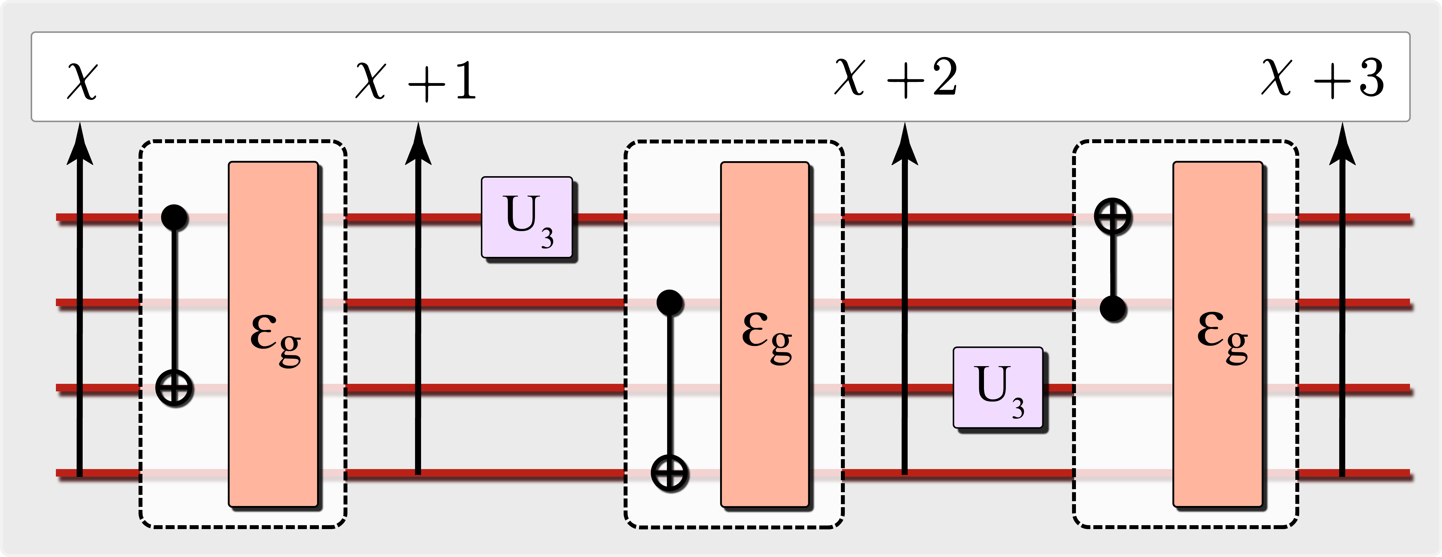
FIG. 1: Depolarizing channels follow CNOT gates.

I.2 The Depolarizing Channel

Depolarization results in the mixing of a quantum state with the infinite temperature Gibbs state, one for which all micro-states are equally likely [72]. Such processes are described by the $n$-qubit depolarizing channel:

$$\hat{\mathcal{D}}_{\epsilon,n}\kern 1.66672pt\rho=(1-\epsilon)\kern 1.00006pt\rho+\epsilon\kern 1.66672pt\mathscr{I}_{n}$$ (I.5)

where $\mathscr{I}_{n}=\mathbbm{1}/2^{n}$ is the infinite temperature state (ITS) and $\epsilon$ is the noise strength.

The repeated action of the depolarizing channel is the following:

$$\hat{\mathcal{D}}^{k}_{\epsilon,n}\kern 1.00006pt\rho =(1-\epsilon)^{k}\kern 1.00006pt\rho+f(\epsilon,k)\kern 1.00006pt\mathscr{I}_{n}$$ (I.6)

$$f (\epsilon,k)=\epsilon\sum_{n=0}^{k-1}(1-\epsilon)^{n}$$ (I.7)

The input state is suppressed exponentially, indicating a signal-to-noise problem. After its qubits are saturated by the ITS, a Quantum Processing Unit (QPU) can no longer perform meaningful computation (Figure 2).

I.3 Proving the Global White-Noise Model

A QPU is composed of qubits coupled to the environment and a measurement apparatus:

$$\mathcal{H}_{\text{\tiny{QPU}}}=\mathcal{H}_{\text{\tiny env}}\otimes\mathcal{H}_{\text{\tiny q}}\otimes\mathcal{H}_{\text{\tiny app}}$$ (I.8)

In the QPU’s expanded Hilbert space, noise dynamics map onto unitary time evolution [73].

Consider a QPU that performs digital computations with CNOT gates. It is examined throughout a quantum computation obeying the computational cycle:

(I.) state preparation: The qubits are prepared in a pure initial state.

(II.) quantum computation: The target computation is performed by applying CNOT gates to the qubits.

(III.) measurement: An observable on $\mathcal{H}_{\text{\tiny q}}$ is measured.

The computational cycle is repeated $N_{m}$ times. Within the QPU, the entire computation is described by unitary evolution for time $t_{\text{\tiny exp}}={\tiny{N_{m}}\kern 0.50003ptt_{\text{\tiny cycle}}}$:

$$\rho_{\text{\tiny{QPU}}}^{(t)}=\hat{U}_{\text{\tiny{QPU}}}^{(t)}\kern 1.00006pt\rho_{\text{\tiny{QPU}}}^{(0)}$$ (I.9)

A location metric is required to identify the occurrence of CNOT gates in a computation. In this work, the scalar depth ($\textstyle\chi$) is used: the number of entangling operations applied after state preparation.

The state of the QPU during the computation can be parametrized by the scalar depth ${\mathchoice{\raisebox{0.0pt}{$\displaystyle\chi$}}{\raisebox{0.0pt}{$\textstyle\chi$}}{\raisebox{0.0pt}{$\scriptstyle\chi$}}{\raisebox{0.0pt}{$\scriptscriptstyle\chi$}}}(t)$:

$$\rho_{\text{\tiny{QPU}}}^{(t)}\rightarrow\rho_{\text{\tiny{QPU}}}[{\mathchoice{\raisebox{0.0pt}{$\displaystyle\chi$}}{\raisebox{0.0pt}{$\textstyle\chi$}}{\raisebox{0.0pt}{$\scriptstyle\chi$}}{\raisebox{0.0pt}{$\scriptscriptstyle\chi$}}}(t)]$$ (I.10)

The qubits will be acted on by the ${\mathchoice{\raisebox{0.0pt}{$\displaystyle\chi$}}{\raisebox{0.0pt}{$\textstyle\chi$}}{\raisebox{0.0pt}{$\scriptstyle\chi$}}{\raisebox{0.0pt}{$\scriptscriptstyle\chi$}}}^{\prime\kern 0.63004pt\text{\tiny th}}$ CNOT gate at times $\{t_{\sigma}\}$ satisfying ${\mathchoice{\raisebox{0.0pt}{$\displaystyle\chi$}}{\raisebox{0.0pt}{$\textstyle\chi$}}{\raisebox{0.0pt}{$\scriptstyle\chi$}}{\raisebox{0.0pt}{$\scriptscriptstyle\chi$}}}(t_{\sigma})={\mathchoice{\raisebox{0.0pt}{$\displaystyle\chi$}}{\raisebox{0.0pt}{$\textstyle\chi$}}{\raisebox{0.0pt}{$\scriptstyle\chi$}}{\raisebox{0.0pt}{$\scriptscriptstyle\chi$}}}^{\prime}$. The state of the QPU at times $\{t_{\sigma}\}$ defines a set of encountering states:

$$\rho_{\text{\tiny{QPU}}}^{(t_{k})}[{\mathchoice{\raisebox{0.0pt}{$\displaystyle\chi$}}{\raisebox{0.0pt}{$\textstyle\chi$}}{\raisebox{0.0pt}{$\scriptstyle\chi$}}{\raisebox{0.0pt}{$\scriptscriptstyle\chi$}}}^{\prime}]=\rho_{\text{\tiny{QPU}}}[{\mathchoice{\raisebox{0.0pt}{$\displaystyle\chi$}}{\raisebox{0.0pt}{$\textstyle\chi$}}{\raisebox{0.0pt}{$\scriptstyle\chi$}}{\raisebox{0.0pt}{$\scriptscriptstyle\chi$}}}^{\prime}(t_{k})]$$ (I.11)

Encountering states at times $t_{l}$ and $t_{k}$ are related by unitary evolution on $\mathcal{H}_{\text{\tiny{QPU}}}$, represented by encountering transformations:

$$\hat{U}_{lk} =\hat{U}_{\text{\tiny{QPU}}}^{(t_{l})}\kern 1.66672pt\hat{U}_{\text{\tiny{QPU}}}^{\dagger(t_{k})}$$ (I.12)

$$\rho_{\text{\tiny{QPU}}}^{(t_{l})}[{\mathchoice{\raisebox{0.0pt}{$\displaystyle\chi$}}{\raisebox{0.0pt}{$\textstyle\chi$}}{\raisebox{0.0pt}{$\scriptstyle\chi$}}{\raisebox{0.0pt}{$\scriptscriptstyle\chi$}}}^{\prime}] =\hat{U}_{lk}\kern 1.66672pt\rho_{\text{\tiny{QPU}}}^{(t_{k})}[{\mathchoice{\raisebox{0.0pt}{$\displaystyle\chi$}}{\raisebox{0.0pt}{$\textstyle\chi$}}{\raisebox{0.0pt}{$\scriptstyle\chi$}}{\raisebox{0.0pt}{$\scriptscriptstyle\chi$}}}^{\prime}]$$ (I.13)

The action of the ${\mathchoice{\raisebox{0.0pt}{$\displaystyle\chi$}}{\raisebox{0.0pt}{$\textstyle\chi$}}{\raisebox{0.0pt}{$\scriptstyle\chi$}}{\raisebox{0.0pt}{$\scriptscriptstyle\chi$}}}^{\prime\text{\tiny th}}$ CNOT gate on the encountering states is treated with quantum channel technology. The native CNOT gate coupling qubits $\small{\{i,j}\}$ is the following:

$$\hat{\mathds{C}}^{ij}_{{\mathchoice{\raisebox{0.0pt}{$\displaystyle\chi$}}{\raisebox{0.0pt}{$\textstyle\chi$}}{\raisebox{0.0pt}{$\scriptstyle\chi$}}{\raisebox{0.0pt}{$\scriptscriptstyle\chi$}}}^{\prime}}=\hat{\mathcal{E}}_{{\mathchoice{\raisebox{0.0pt}{$\displaystyle\chi$}}{\raisebox{0.0pt}{$\textstyle\chi$}}{\raisebox{0.0pt}{$\scriptstyle\chi$}}{\raisebox{0.0pt}{$\scriptscriptstyle\chi$}}}^{\prime}}\kern 1.00006pt\hat{C}^{ij}_{x}$$ (I.14)

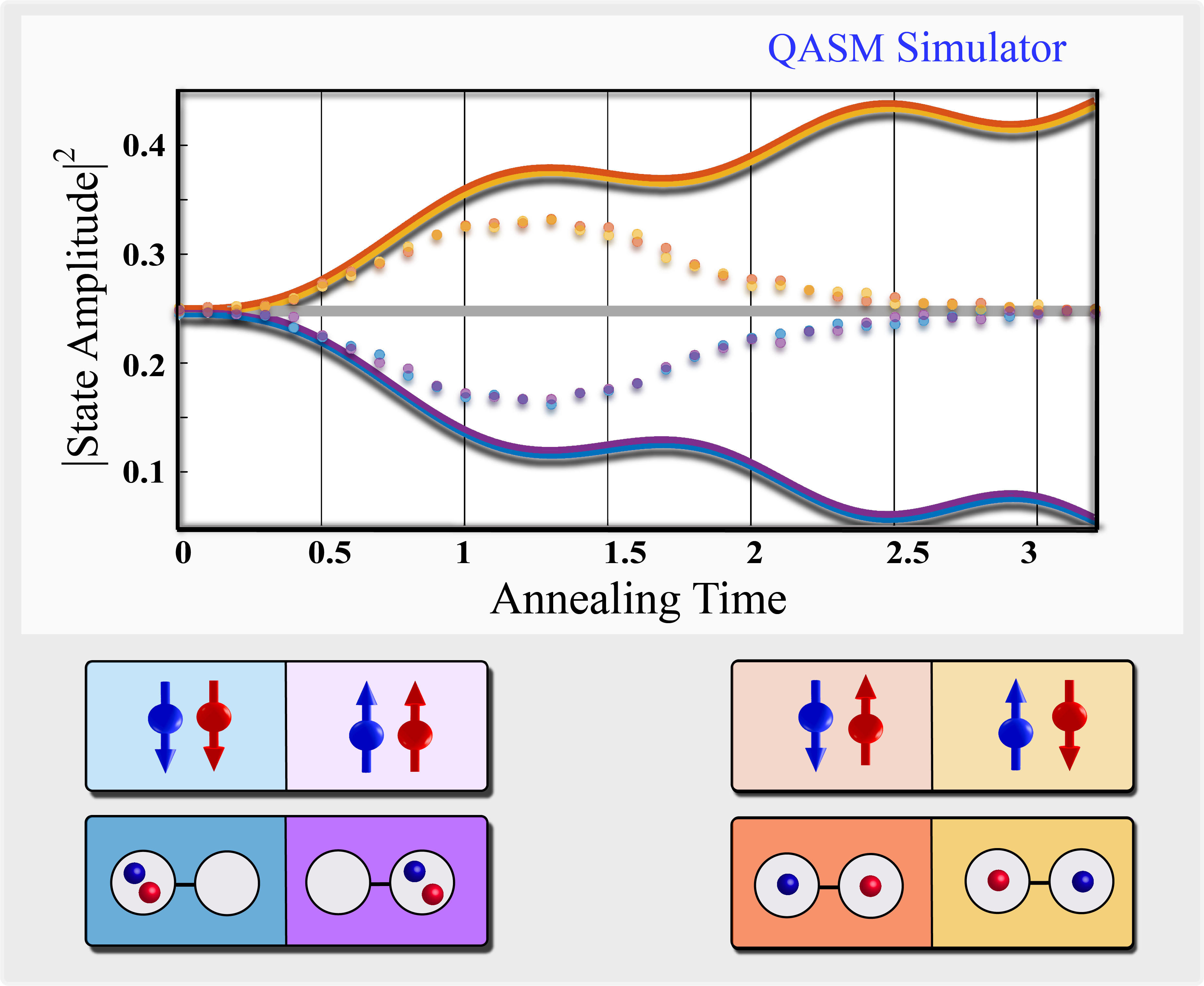
FIG. 2: The time evolution of the Fermi-Hubbard Model is computed numerically (solid). Depolarizing noise dynamics (circles) cause saturation with the ITS (grey).

$\hat{\mathcal{E}}_{{\mathchoice{\raisebox{0.0pt}{$\displaystyle\chi$}}{\raisebox{0.0pt}{$\textstyle\chi$}}{\raisebox{0.0pt}{$\scriptstyle\chi$}}{\raisebox{0.0pt}{$\scriptscriptstyle\chi$}}}^{\prime}}$ is a superoperator describing the noise dynamics of the native gate. $C^{ij}_{x}$ is the ideal CNOT gate.

To treat the noise dynamics in a unitary fashion, a Stinespring dilation [74] is performed:

$$\mathcal{H}_{\text{\tiny q}}\rightarrow\mathcal{H}_{\text{\tiny{QPU}}},\ \ \hat{\mathcal{E}}_{{\mathchoice{\raisebox{0.0pt}{$\displaystyle\chi$}}{\raisebox{0.0pt}{$\textstyle\chi$}}{\raisebox{0.0pt}{$\scriptstyle\chi$}}{\raisebox{0.0pt}{$\scriptscriptstyle\chi$}}}^{\prime}}\rightarrow\hat{V}_{{\mathchoice{\raisebox{0.0pt}{$\displaystyle\chi$}}{\raisebox{0.0pt}{$\textstyle\chi$}}{\raisebox{0.0pt}{$\scriptstyle\chi$}}{\raisebox{0.0pt}{$\scriptscriptstyle\chi$}}}^{\prime}}\kern 1.66672pt\hat{\xi}$$ (I.15)

$\hat{\xi}$ is a unital homomorphism that takes $\mathcal{H}_{\text{\tiny q}}\kern-1.34995pt\rightarrow\mathcal{H}_{\text{\tiny{QPU}}}$. $\hat{V}_{{\mathchoice{\raisebox{0.0pt}{$\displaystyle\chi$}}{\raisebox{0.0pt}{$\textstyle\chi$}}{\raisebox{0.0pt}{$\scriptstyle\chi$}}{\raisebox{0.0pt}{$\scriptscriptstyle\chi$}}}^{\prime}}$ is a unitary transformation acting on $\mathcal{H}_{\text{\tiny{QPU}}}$.

The action of $\hat{\mathds{C}}^{ij}_{{\mathchoice{\raisebox{0.0pt}{$\displaystyle\chi$}}{\raisebox{0.0pt}{$\textstyle\chi$}}{\raisebox{0.0pt}{$\scriptstyle\chi$}}{\raisebox{0.0pt}{$\scriptscriptstyle\chi$}}}^{\prime}}$ on the $k^{\text{th}}$ encountering state is as follows:

$$\rho_{\text{\tiny{QPU}}}^{(t_{k})}[{\mathchoice{\raisebox{0.0pt}{$\displaystyle\chi$}}{\raisebox{0.0pt}{$\textstyle\chi$}}{\raisebox{0.0pt}{$\scriptstyle\chi$}}{\raisebox{0.0pt}{$\scriptscriptstyle\chi$}}}^{\prime}\small{+}1]=\hat{V}_{{\mathchoice{\raisebox{0.0pt}{$\displaystyle\chi$}}{\raisebox{0.0pt}{$\textstyle\chi$}}{\raisebox{0.0pt}{$\scriptstyle\chi$}}{\raisebox{0.0pt}{$\scriptscriptstyle\chi$}}}^{\prime}}\kern 0.90005pt\kern 0.90005pt\hat{C}^{ij}_{x}\kern 1.50005pt\rho_{\text{\tiny{QPU}}}^{(t_{k})}[{\mathchoice{\raisebox{0.0pt}{$\displaystyle\chi$}}{\raisebox{0.0pt}{$\textstyle\chi$}}{\raisebox{0.0pt}{$\scriptstyle\chi$}}{\raisebox{0.0pt}{$\scriptscriptstyle\chi$}}}^{\prime}]$$ (I.16)

The expectation value of $O_{\text{\tiny q}}$ is obtained by averaging the contributions of the encountering states:

$$\begin{split}\braket{O_{\text{\tiny q}}}&=\frac{1}{N_{m}}\sum_{k=1}^{N_{m}}\text{Tr}_{\text{\tiny{QPU}}}\Big{[}\Big{\{}\hat{V}_{{\mathchoice{\raisebox{0.0pt}{$\displaystyle\chi$}}{\raisebox{0.0pt}{$\textstyle\chi$}}{\raisebox{0.0pt}{$\scriptstyle\chi$}}{\raisebox{0.0pt}{$\scriptscriptstyle\chi$}}}^{\prime}}\kern 1.00006pt\kern 1.00006pt\hat{C}^{ij}_{x}\kern 1.66672pt\rho_{\text{\tiny{QPU}}}^{(t_{k})}[{\mathchoice{\raisebox{0.0pt}{$\displaystyle\chi$}}{\raisebox{0.0pt}{$\textstyle\chi$}}{\raisebox{0.0pt}{$\scriptstyle\chi$}}{\raisebox{0.0pt}{$\scriptscriptstyle\chi$}}}^{\prime}]\Big{\}}\kern 1.66672ptO_{\text{\tiny q}}\Big{]}\\ &=\frac{1}{N_{m}}\sum_{k=1}^{N_{m}}\text{Tr}_{\text{\tiny{QPU}}}\Big{[}\Big{\{}\hat{V}_{{\mathchoice{\raisebox{0.0pt}{$\displaystyle\chi$}}{\raisebox{0.0pt}{$\textstyle\chi$}}{\raisebox{0.0pt}{$\scriptstyle\chi$}}{\raisebox{0.0pt}{$\scriptscriptstyle\chi$}}}^{\prime}}\kern 1.00006pt\kern 1.00006pt\hat{C}^{ij}_{x}\kern 1.66672pt\hat{U}_{k1}\kern 1.00006pt\rho_{\text{\tiny{QPU}}}^{(t_{1})}[{\mathchoice{\raisebox{0.0pt}{$\displaystyle\chi$}}{\raisebox{0.0pt}{$\textstyle\chi$}}{\raisebox{0.0pt}{$\scriptstyle\chi$}}{\raisebox{0.0pt}{$\scriptscriptstyle\chi$}}}^{\prime}]\Big{\}}\kern 1.66672ptO_{\text{\tiny q}}\Big{]}\end{split}$$ (I.17)

In the second line, $\rho_{\text{\tiny{QPU}}}^{(t_{k})}[{\mathchoice{\raisebox{0.0pt}{$\displaystyle\chi$}}{\raisebox{0.0pt}{$\textstyle\chi$}}{\raisebox{0.0pt}{$\scriptstyle\chi$}}{\raisebox{0.0pt}{$\scriptscriptstyle\chi$}}}^{\prime}]$ is expressed in terms of an encountering transformation on $\rho_{\text{\tiny{QPU}}}^{(t_{1})}[{\mathchoice{\raisebox{0.0pt}{$\displaystyle\chi$}}{\raisebox{0.0pt}{$\textstyle\chi$}}{\raisebox{0.0pt}{$\scriptstyle\chi$}}{\raisebox{0.0pt}{$\scriptscriptstyle\chi$}}}^{\prime}]$.

In the ideal limit, the target computation is applied identically for all cycles. This implies the following:

$$\big{[}O_{\text{\tiny q}},U^{\text{\tiny{ideal}}}_{lk}\big{]}=0$$ (I.18)

$U_{{}_{k1}}U^{\text{\tiny$\dagger$}}_{k1}$ is now inserted into Equation I.17:

$$\begin{split}\braket{O_{\text{\tiny q}}}=\frac{1}{N_{m}}\sum_{k=1}^{N_{m}}\text{Tr}_{\text{\tiny{QPU}}}\Big{[}\kern 1.00006ptU^{\dagger}_{k1}\Big{\{}\hat{V}_{{\mathchoice{\raisebox{0.0pt}{$\displaystyle\chi$}}{\raisebox{0.0pt}{$\textstyle\chi$}}{\raisebox{0.0pt}{$\scriptstyle\chi$}}{\raisebox{0.0pt}{$\scriptscriptstyle\chi$}}}^{\prime}}\kern 1.00006pt\kern 1.00006pt\hat{C}^{ij}_{x}\kern 1.66672pt\hat{U}_{k1}\kern 1.00006pt\rho_{\text{\tiny{QPU}}}^{(t_{1})}[{\mathchoice{\raisebox{0.0pt}{$\displaystyle\chi$}}{\raisebox{0.0pt}{$\textstyle\chi$}}{\raisebox{0.0pt}{$\scriptstyle\chi$}}{\raisebox{0.0pt}{$\scriptscriptstyle\chi$}}}^{\prime}]\Big{\}}\kern 1.00006ptO_{\text{\tiny q}}\kern 1.00006pt\text{$U_{k1}$}\Big{]}\\ \approx\frac{1}{N_{m}}\sum_{k=1}^{N_{m}}\text{Tr}_{\text{\tiny{QPU}}}\Big{[}\kern 1.00006ptU^{\dagger}_{k1}\Big{\{}\kern 1.00006pt\hat{V}_{{\mathchoice{\raisebox{0.0pt}{$\displaystyle\chi$}}{\raisebox{0.0pt}{$\textstyle\chi$}}{\raisebox{0.0pt}{$\scriptstyle\chi$}}{\raisebox{0.0pt}{$\scriptscriptstyle\chi$}}}^{\prime}}\kern 1.00006pt\text{$\hat{U}_{k1}$}\kern 1.66672pt\hat{C}^{ij}_{x}\kern 1.00006pt\rho_{\text{\tiny{QPU}}}^{(t_{1})}[{\mathchoice{\raisebox{0.0pt}{$\displaystyle\chi$}}{\raisebox{0.0pt}{$\textstyle\chi$}}{\raisebox{0.0pt}{$\scriptstyle\chi$}}{\raisebox{0.0pt}{$\scriptscriptstyle\chi$}}}^{\prime}]\Big{\}}\kern 1.66672pt\text{$U_{k1}$}\kern 1.66672ptO_{\text{\tiny q}}\Big{]}\end{split}$$ (I.19)

This allows Equation I.19 to be expressed as follows:

$$\begin{split}\braket{O_{\text{\tiny q}}}&\approx\frac{1}{N_{m}}\sum_{k=1}^{N_{m}}\text{Tr}_{\text{\tiny{QPU}}}\Big{[}\kern 1.00006pt\Big{\{}\hat{U}^{\dagger}_{k1}\kern 1.00006pt\hat{V}_{{\mathchoice{\raisebox{0.0pt}{$\displaystyle\chi$}}{\raisebox{0.0pt}{$\textstyle\chi$}}{\raisebox{0.0pt}{$\scriptstyle\chi$}}{\raisebox{0.0pt}{$\scriptscriptstyle\chi$}}}^{\prime}}\kern 1.00006pt\kern 1.66672pt\text{$\hat{U}_{k1}$}\ \kern 1.00006pt\hat{C}^{ij}_{x}\kern 1.66672pt\rho_{\text{\tiny{QPU}}}^{(t_{1})}[{\mathchoice{\raisebox{0.0pt}{$\displaystyle\chi$}}{\raisebox{0.0pt}{$\textstyle\chi$}}{\raisebox{0.0pt}{$\scriptstyle\chi$}}{\raisebox{0.0pt}{$\scriptscriptstyle\chi$}}}^{\prime}]\Big{\}}\kern 1.66672ptO_{\text{\tiny q}}\Big{]}\end{split}$$ (I.20)

Note the following identity [75]:

$$\begin{split}\mathcal{E}^{\text{\tiny ave}}\rho&=\int dU\kern 1.66672pt\hat{U}^{\dagger}\kern 1.00006pt\hat{\mathcal{E}}\kern 1.00006pt\hat{U}\kern 1.66672pt\rho\\ &=(1-\epsilon)\kern 1.00006pt\rho+\epsilon\kern 1.00006pt\mathscr{I}_{n}\end{split}$$ (I.21)

Applying this relation yields the following:

$$\braket{O_{\text{\tiny q}}} \sim\int dU\kern 1.66672pt\text{Tr}_{\text{\tiny{QPU}}}\Big{[}\Big{\{}\kern 1.66672pt\hat{U}^{\dagger}\kern 1.66672pt\hat{V}_{{\mathchoice{\raisebox{0.0pt}{$\displaystyle\chi$}}{\raisebox{0.0pt}{$\textstyle\chi$}}{\raisebox{0.0pt}{$\scriptstyle\chi$}}{\raisebox{0.0pt}{$\scriptscriptstyle\chi$}}}^{\prime}}\kern 1.66672pt\hat{U}\ \hat{C}^{ij}_{x}\rho_{\text{\tiny{QPU}}}^{(t_{1})}[{\mathchoice{\raisebox{0.0pt}{$\displaystyle\chi$}}{\raisebox{0.0pt}{$\textstyle\chi$}}{\raisebox{0.0pt}{$\scriptstyle\chi$}}{\raisebox{0.0pt}{$\scriptscriptstyle\chi$}}}^{\prime}]\Big{\}}\kern 1.66672ptO_{\text{\tiny q}}\Big{]}$$

$$=\kern 1.66672pt\text{Tr}_{\text{\tiny q}}\Big{[}\Big{\{}(1-\epsilon_{g})\kern 1.66672pt\hat{C}^{ij}_{x}\rho_{\text{\tiny q}}[{\mathchoice{\raisebox{0.0pt}{$\displaystyle\chi$}}{\raisebox{0.0pt}{$\textstyle\chi$}}{\raisebox{0.0pt}{$\scriptstyle\chi$}}{\raisebox{0.0pt}{$\scriptscriptstyle\chi$}}}^{\prime}]+\epsilon_{g}\kern 1.66672pt\mathscr{I}_{n}\Big{\}}\kern 1.66672ptO_{\text{\tiny q}}\Big{]}$$ (I.22)

The averaged noise dynamics of the CNOT gate approximate a global depolarizing channel with global noise strength $\epsilon_{g}$.

The noise dynamics of the CNOT gate can be modified using noise tailoring (NT) algorithms (Appendix I).

II CLAssical White-noise Extrapolation

The objective of CLAssical White-noise Extrapolation (CLAWE) [29], is the extraction of ideal observables from their noisy counterparts. This extraction requires the noise dynamics to obey the global white-noise model.

II.1 Model-Based Extrapolation

CLAWE is a model-based extrapolation algorithm. Model-based extrapolation [76, 77, 78, 79] can be represented schematically in three stages:

1. Modeling: Find a suitable model that describes a class of systems $\{\mathcal{P}_{\sigma}\}$, using parameters $\{\lambda_{\alpha}\}$. The model must relate accessible observables to target observables: $\{\braket{O^{\text{\tiny acc}}_{\mu}}\}\rightarrow\{\braket{O_{\nu}^{\text{\tiny targ}}}\}$.

2. Calibration: Determine the model parameters $\{\lambda_{\alpha}^{\text{\tiny exp}}\}$ for a system $\mathcal{P}_{\text{phys}}$, by measuring calibration observables $\{\braket{O_{\gamma}^{\text{\tiny cal}}}\}$.

3. Extrapolation: Use the model to estimate target observables of $\mathcal{P}_{\text{phys}}$.

II.1.1 Modeling

Model Inversion: It is possible to exactly invert the global white-noise model due to the unitary invariance of the depolarizing channel:

$$\hat{\mathcal{D}}_{\epsilon,n}\kern 1.00006pt\hat{U}\kern 1.66672pt\rho\kern 1.66672pt=\kern 1.66672pt\hat{U}\kern 1.66672pt\hat{\mathcal{D}}_{\epsilon,n}\kern 1.66672pt\rho$$ (II.1)

Consider a target computation of scalar depth $\textstyle\chi$: $U_{{}_{{\mathchoice{\raisebox{0.0pt}{$\displaystyle\chi$}}{\raisebox{0.0pt}{$\textstyle\chi$}}{\raisebox{0.0pt}{$\scriptstyle\chi$}}{\raisebox{0.0pt}{$\scriptscriptstyle\chi$}}}}}$. There are $\textstyle\chi$ global depolarizing channels dressing the ideal gates, which can be moved to the end of the computation, such that they act on the perfect output state:

$${\rho_{{}_{\kern-0.74997ptn}}=(1-\epsilon_{g})^{{\mathchoice{\raisebox{0.0pt}{$\displaystyle\chi$}}{\raisebox{0.0pt}{$\textstyle\chi$}}{\raisebox{0.0pt}{$\scriptstyle\chi$}}{\raisebox{0.0pt}{$\scriptscriptstyle\chi$}}}}\kern 1.66672pt\kern 1.00006pt\text{{\hbox{\hat{U}_{\kern-1.00006pt\scalebox{0.6}{}}}}}}\kern 1.00006pt\rho+f(\epsilon_{g},{\mathchoice{\raisebox{0.0pt}{$\displaystyle\chi$}}{\raisebox{0.0pt}{$\textstyle\chi$}}{\raisebox{0.0pt}{$\scriptstyle\chi$}}{\raisebox{0.0pt}{$\scriptscriptstyle\chi$}}})\kern 1.66672pt\mathscr{I}_{n}.$$ (II.2)

This relation can be used to express a noisy observable in terms of its infinite temperature value $\Omega_{ITS}=\text{\normalsize{Tr}}[\kern 0.90005pt\mathscr{I}_{n}\kern 0.90005ptO]$:

$$\begin{split}\braket{O_{{}_{\kern-0.74997ptn}}}&=(1-\epsilon_{g})^{{\mathchoice{\raisebox{0.0pt}{$\displaystyle\chi$}}{\raisebox{0.0pt}{$\textstyle\chi$}}{\raisebox{0.0pt}{$\scriptstyle\chi$}}{\raisebox{0.0pt}{$\scriptscriptstyle\chi$}}}}\ \scalebox{1.1}{$\text{Tr}$}\big{[}\kern 1.00006pt\text{$\hat{U}_{\kern-0.70004pt\scalebox{0.6}{${\mathchoice{\raisebox{0.0pt}{$\displaystyle\chi$}}{\raisebox{0.0pt}{$\textstyle\chi$}}{\raisebox{0.0pt}{$\scriptstyle\chi$}}{\raisebox{0.0pt}{$\scriptscriptstyle\chi$}}}$}}$}\kern 0.70007pt\rho\kern 1.00006pt\kern 0.70007ptO\kern 0.70007pt\big{]}+f(\epsilon_{g},{\mathchoice{\raisebox{0.0pt}{$\displaystyle\chi$}}{\raisebox{0.0pt}{$\textstyle\chi$}}{\raisebox{0.0pt}{$\scriptstyle\chi$}}{\raisebox{0.0pt}{$\scriptscriptstyle\chi$}}})\kern 1.66672pt\scalebox{1.1}{$\text{Tr}$}\big{[}\kern 1.00006pt\mathscr{I}_{n}O\kern 0.70007pt\big{]}\\ &=(1-\epsilon_{g})^{{\mathchoice{\raisebox{0.0pt}{$\displaystyle\chi$}}{\raisebox{0.0pt}{$\textstyle\chi$}}{\raisebox{0.0pt}{$\scriptstyle\chi$}}{\raisebox{0.0pt}{$\scriptscriptstyle\chi$}}}}\ \scalebox{1.1}{$\text{Tr}$}\big{[}\kern 1.00006pt\rho\kern 1.00006pt\kern 0.70007pt\text{$\hat{U}_{\kern-0.70004pt\scalebox{0.6}{${\mathchoice{\raisebox{0.0pt}{$\displaystyle\chi$}}{\raisebox{0.0pt}{$\textstyle\chi$}}{\raisebox{0.0pt}{$\scriptstyle\chi$}}{\raisebox{0.0pt}{$\scriptscriptstyle\chi$}}}$}}$}^{\kern-2.10002pt\kern 0.49005pt\dagger}\kern-1.00006ptO\kern 0.70007pt\big{]}+f(\epsilon_{g},{\mathchoice{\raisebox{0.0pt}{$\displaystyle\chi$}}{\raisebox{0.0pt}{$\textstyle\chi$}}{\raisebox{0.0pt}{$\scriptstyle\chi$}}{\raisebox{0.0pt}{$\scriptscriptstyle\chi$}}})\kern 1.66672pt\scalebox{1.1}{$\text{Tr}$}\big{[}\kern 1.00006pt\mathscr{I}_{n}O\kern 0.70007pt\big{]}\\[3.99994pt] &=(1-\epsilon_{g})^{{\mathchoice{\raisebox{0.0pt}{$\displaystyle\chi$}}{\raisebox{0.0pt}{$\textstyle\chi$}}{\raisebox{0.0pt}{$\scriptstyle\chi$}}{\raisebox{0.0pt}{$\scriptscriptstyle\chi$}}}}\Braket{\text{$\hat{U}_{\kern-0.70004pt\scalebox{0.6}{${\mathchoice{\raisebox{0.0pt}{$\displaystyle\chi$}}{\raisebox{0.0pt}{$\textstyle\chi$}}{\raisebox{0.0pt}{$\scriptstyle\chi$}}{\raisebox{0.0pt}{$\scriptscriptstyle\chi$}}}$}}$}^{\kern-2.10002pt\kern 0.49005pt\dagger}O}+f(\epsilon_{g},{\mathchoice{\raisebox{0.0pt}{$\displaystyle\chi$}}{\raisebox{0.0pt}{$\textstyle\chi$}}{\raisebox{0.0pt}{$\scriptstyle\chi$}}{\raisebox{0.0pt}{$\scriptscriptstyle\chi$}}})\kern 1.66672pt\Omega_{ITS}\\[3.99994pt] &=(1-\epsilon_{g})^{{\mathchoice{\raisebox{0.0pt}{$\displaystyle\chi$}}{\raisebox{0.0pt}{$\textstyle\chi$}}{\raisebox{0.0pt}{$\scriptstyle\chi$}}{\raisebox{0.0pt}{$\scriptscriptstyle\chi$}}}}\braket{\kern 0.70007ptO_{\kern-0.70004ptu}\kern 0.70007pt}+f(\epsilon_{g},{\mathchoice{\raisebox{0.0pt}{$\displaystyle\chi$}}{\raisebox{0.0pt}{$\textstyle\chi$}}{\raisebox{0.0pt}{$\scriptstyle\chi$}}{\raisebox{0.0pt}{$\scriptscriptstyle\chi$}}})\kern 1.66672pt\Omega_{ITS}\end{split}$$ (II.3)

Apply the geometric sum formula to $f(\epsilon_{g},{\mathchoice{\raisebox{0.0pt}{$\displaystyle\chi$}}{\raisebox{0.0pt}{$\textstyle\chi$}}{\raisebox{0.0pt}{$\scriptstyle\chi$}}{\raisebox{0.0pt}{$\scriptscriptstyle\chi$}}})$ (Equation I.7), to isolate the ideal observable $\braket{O_{u}}$:

$$\begin{split}\braket{O_{{}_{\kern-1.50002ptn}}}=(1-\epsilon_{g})^{{\mathchoice{\raisebox{0.0pt}{$\displaystyle\chi$}}{\raisebox{0.0pt}{$\textstyle\chi$}}{\raisebox{0.0pt}{$\scriptstyle\chi$}}{\raisebox{0.0pt}{$\scriptscriptstyle\chi$}}}}&\braket{\kern 0.70007ptO_{\kern-0.70004ptu}\kern 0.70007pt}+\big{[}1-(1-\epsilon_{g})^{{\mathchoice{\raisebox{0.0pt}{$\displaystyle\chi$}}{\raisebox{0.0pt}{$\textstyle\chi$}}{\raisebox{0.0pt}{$\scriptstyle\chi$}}{\raisebox{0.0pt}{$\scriptscriptstyle\chi$}}}}\kern 0.70007pt\big{]}\kern 1.66672pt\Omega_{ITS}\\[6.00006pt] \braket{O_{{}_{\kern-1.50002ptn}}}-\Omega_{ITS}&=(1-\epsilon_{g})^{{\mathchoice{\raisebox{0.0pt}{$\displaystyle\chi$}}{\raisebox{0.0pt}{$\textstyle\chi$}}{\raisebox{0.0pt}{$\scriptstyle\chi$}}{\raisebox{0.0pt}{$\scriptscriptstyle\chi$}}}}\kern 1.00006pt\big{[}\kern-1.00006pt\braket{\kern 0.70007ptO_{\kern-0.70004ptu}\kern 0.70007pt}-\Omega_{ITS}\kern 0.70007pt\big{]}\end{split}$$ (II.4)

To obtain a simple relation, the rescaled observable is defined $\Omega\equiv O-\Omega_{ITS}\kern-1.34995pt\times\kern-1.34995pt\mathscr{I}_{n}$:

$$\braket{\Omega_{n}}=\text{{\hbox{(1-\epsilon_g)^{\kern 0.70007pt{\mathchoice{\raisebox{0.0pt}{$\displaystyle\chi$}}{\raisebox{0.0pt}{$\textstyle\chi$}}{\raisebox{0.0pt}{$\scriptstyle\chi$}}{\raisebox{0.0pt}{$\scriptscriptstyle\chi$}}}}}}}\braket{\Omega_{u}}$$ (II.5)

II.1.2 Calibration

A calibrating unitary is a secondary computation that mimics the noise dynamics of the primary computation. It must have a calibrating observable: a quantity whose ideal observable $\braket{O^{c}_{u}}$ is known for a calibration state $\rho_{{}_{\kern-0.67497ptc}}$.

To obtain $\braket{O^{c}_{n}}$, the calibrating observable is measured after applying the calibrating unitary to $\rho_{{}_{\kern-0.67497ptc}}$. Taking the ratio of the noisy observable to the ideal observable after rescaling, yields the contamination $\mathcal{C}\text{\footnotesize(${\mathchoice{\raisebox{0.0pt}{$\displaystyle\chi$}}{\raisebox{0.0pt}{$\textstyle\chi$}}{\raisebox{0.0pt}{$\scriptstyle\chi$}}{\raisebox{0.0pt}{$\scriptscriptstyle\chi$}}}_{c}$)}$:

$$\mathcal{C}\text{\footnotesize({\hbox{{\mathchoice{\raisebox{0.0pt}{$\displaystyle\chi$}}{\raisebox{0.0pt}{$\textstyle\chi$}}{\raisebox{0.0pt}{$\scriptstyle\chi$}}{\raisebox{0.0pt}{$\scriptscriptstyle\chi$}}}_c}})}=\frac{\braket{\text{{\hbox{\Omega_n^{c}}}}}}{\braket{\text{{\hbox{{\Omega_u^{c}}}}}}}$$ (II.6)

The secondary global noise strength is given in terms of the contamination:

$${\epsilon^{s}_{g}=1-\text{{\hbox{\mathcal{C}\text{\footnotesize(}}^{1/{\mathchoice{\raisebox{0.0pt}{$\displaystyle\chi$}}{\raisebox{0.0pt}{$\textstyle\chi$}}{\raisebox{0.0pt}{$\scriptstyle\chi$}}{\raisebox{0.0pt}{$\scriptscriptstyle\chi$}}}_c}}}}$$ (II.7)

II.1.3 Extrapolation

The ideal map is the estimate of the ideal observable obtained from CLAWE:

$$\braket{\text{$\Omega^{\kern 0.49005pt\text{\tiny map}}_{u}$}} =(1-\epsilon^{s}_{g}\kern 1.00006pt\text{$)^{\kern-0.70004pt-{\mathchoice{\raisebox{0.0pt}{$\displaystyle\chi$}}{\raisebox{0.0pt}{$\textstyle\chi$}}{\raisebox{0.0pt}{$\scriptstyle\chi$}}{\raisebox{0.0pt}{$\scriptscriptstyle\chi$}}}}$}\braket{\Omega_{n}}$$ (II.8)

$$\braket{\text{$\Omega^{\kern 0.49005pt\text{\tiny map}}_{u}$}} =(1-\epsilon^{s}_{g}\kern 1.00006pt\text{$)^{\kern-0.70004pt-{\mathchoice{\raisebox{0.0pt}{$\displaystyle\chi$}}{\raisebox{0.0pt}{$\textstyle\chi$}}{\raisebox{0.0pt}{$\scriptstyle\chi$}}{\raisebox{0.0pt}{$\scriptscriptstyle\chi$}}}}$}\kern 1.00006pt\kern 0.70007pt\text{$(1-\epsilon_{g})^{{\mathchoice{\raisebox{0.0pt}{$\displaystyle\chi$}}{\raisebox{0.0pt}{$\textstyle\chi$}}{\raisebox{0.0pt}{$\scriptstyle\chi$}}{\raisebox{0.0pt}{$\scriptscriptstyle\chi$}}}}$}\braket{\Omega_{u}}$$ (II.9)

The viability of CLAWE is determined by the ratio of the ideal map to the ideal observable:

$$\frac{\braket{\text{{\hbox{\Omega^{\kern 0.70007pt\text{\tiny map}}_{u}}}}}}{\braket{\Omega_{u}}}=\scalebox{0.9}{{\hbox{\Bigg{(}}}}\frac{1-\epsilon_{g}}{1-\epsilon_{g}^{s}}\scalebox{0.9}{{\hbox{\Bigg{)}}}}^{\kern 0.49005pt{\mathchoice{\raisebox{0.0pt}{$\displaystyle\chi$}}{\raisebox{0.0pt}{$\textstyle\chi$}}{\raisebox{0.0pt}{$\scriptstyle\chi$}}{\raisebox{0.0pt}{$\scriptscriptstyle\chi$}}}}$$ (II.10)

The ratio scales super-polynomially as the scalar depth increases. The ideal map becomes unstable beyond the gate cutoff: ${\mathchoice{\raisebox{0.0pt}{$\displaystyle\chi$}}{\raisebox{0.0pt}{$\textstyle\chi$}}{\raisebox{0.0pt}{$\scriptstyle\chi$}}{\raisebox{0.0pt}{$\scriptscriptstyle\chi$}}}_{\text{g}}\kern 1.50005pt\text{$\scriptstyle{\sim}$}\kern 1.50005pt\mathcal{O}(1/\epsilon_{g})$. This comes as a result of the depolarizing channel’s signal-to-noise problem.

II.2 Calibration Algorithms

In the following algorithms, motion-reversal ($\hat{U}^{\dagger}\hat{U}$) of the target computation is used as the calibrating unitary [26].

II.2.1 Variant I

An implicit assumption of Equation II.5 is that $\epsilon_{g}$ is relatively constant during the course of the computation. The Variant I calibration algorithm is designed to extract this constant, by applying motion-reversal in powers of the target computation (Figure 4):

$$\big{\{}\kern 1.66672pt\hat{U}_{{\mathchoice{\raisebox{0.0pt}{$\displaystyle\chi$}}{\raisebox{0.0pt}{$\textstyle\chi$}}{\raisebox{0.0pt}{$\scriptstyle\chi$}}{\raisebox{0.0pt}{$\scriptscriptstyle\chi$}}}}^{\dagger k}\kern 1.66672pt\kern 1.00006pt\hat{U}_{{\mathchoice{\raisebox{0.0pt}{$\displaystyle\chi$}}{\raisebox{0.0pt}{$\textstyle\chi$}}{\raisebox{0.0pt}{$\scriptstyle\chi$}}{\raisebox{0.0pt}{$\scriptscriptstyle\chi$}}}}^{k}\kern 1.66672pt\kern 1.00006pt\big{|}\scalebox{0.9}{\kern 1.66672pt\kern 1.00006ptfor {\hbox{\forall}} \kern 1.66672pt{\hbox{k}}, from {\hbox{1}} to {\hbox{N_c}}}\big{\}}\kern-1.49994pt\kern-6.00006pt\kern-6.00006pt\kern-6.00006pt$$ (II.11)

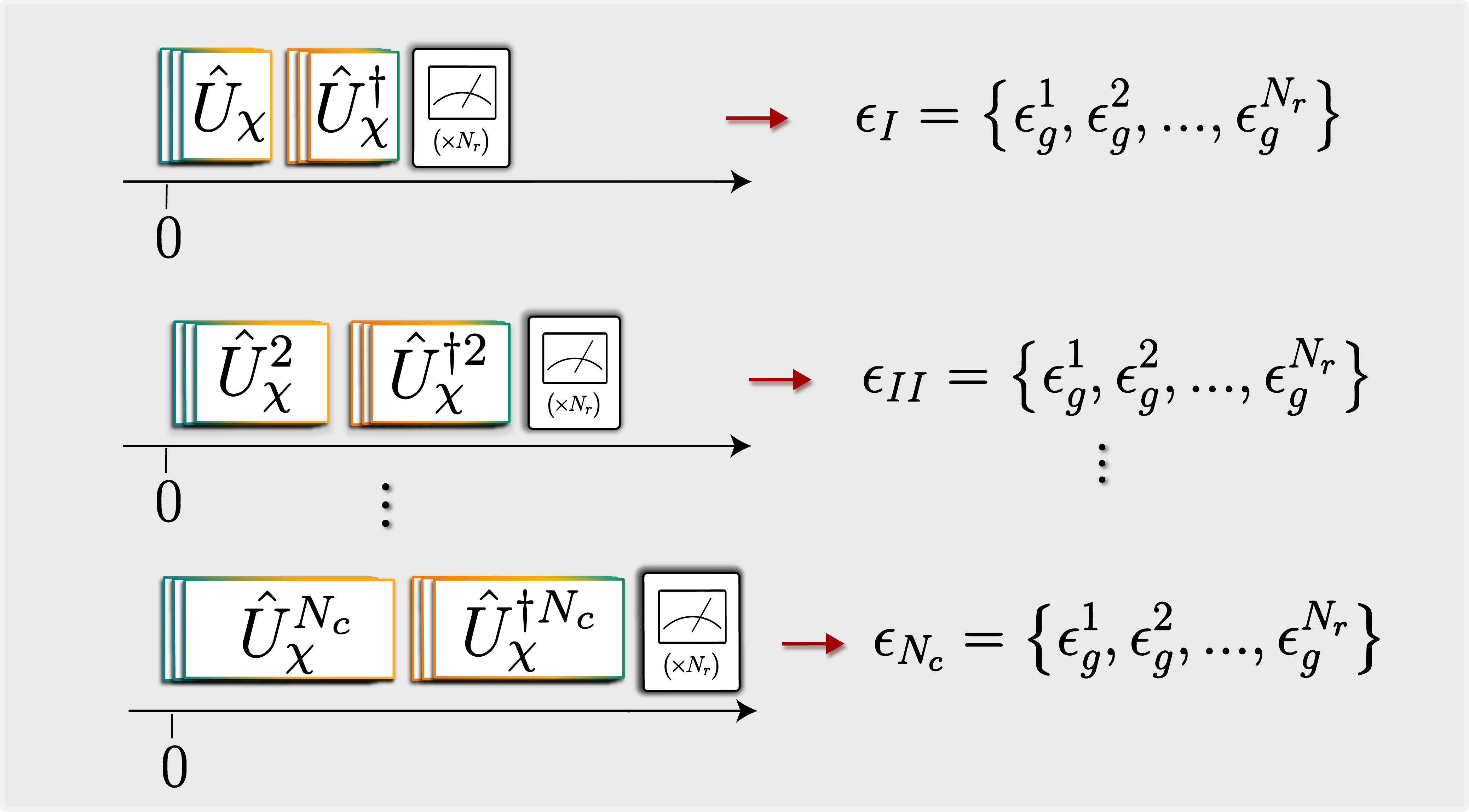
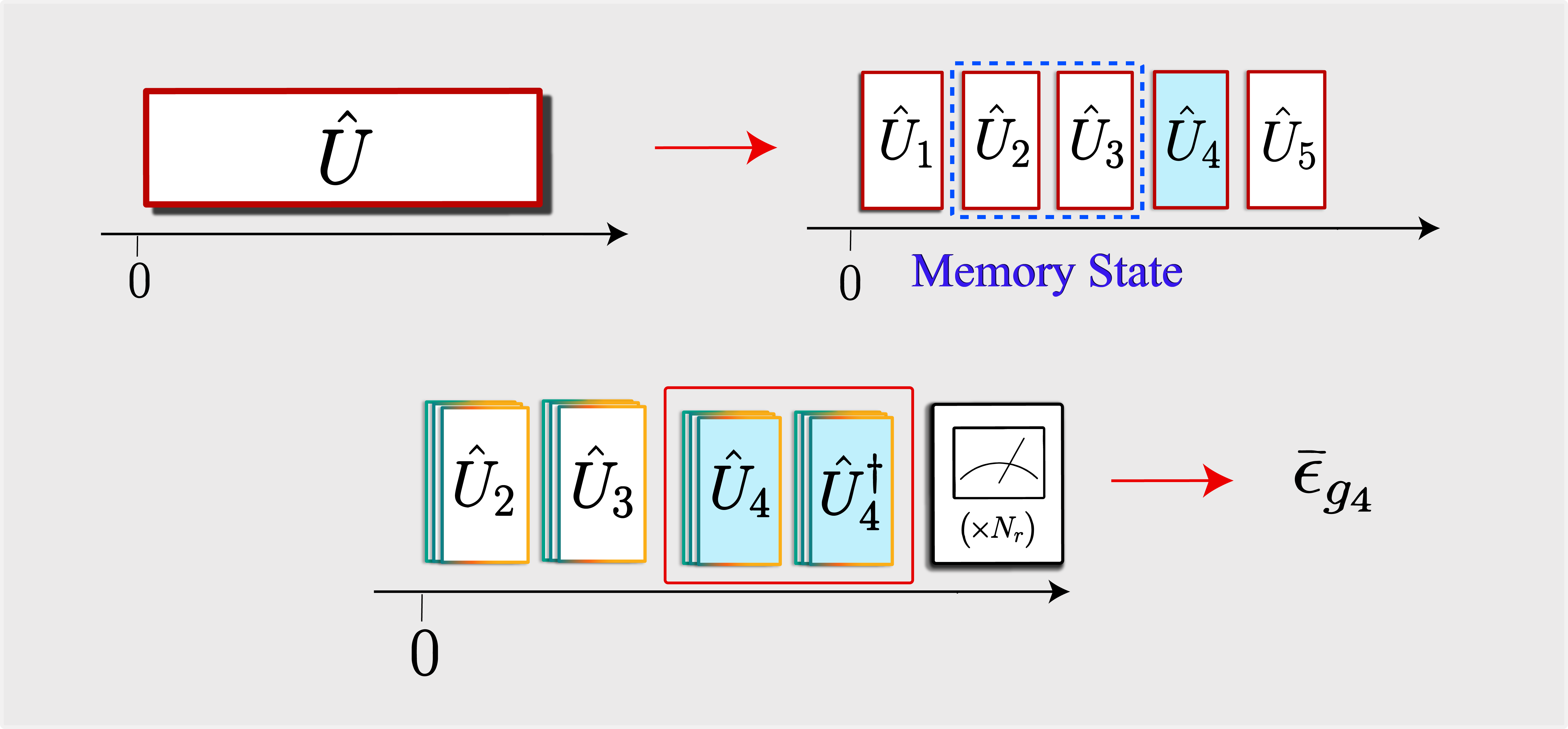
FIG. 3: Variant I: A series of noise-tailored, motion-reversal experiments is performed. Measuring the contamination generates estimates of $\epsilon_{g}$.

FIG. 4: Variant II: [Upper panel] A target computation is partitioned into unitary fragments. A memory window (dashed) is used to generate the memory state. [Lower panel] Applying motion-reversal to the memory state with $U_{4}$ generates estimates of $\epsilon_{g_{4}}$.

II.2.2 Variant II

The Variant II calibration algorithm partitions the target computation into unitary fragments of scalar depth $\{{\mathchoice{\raisebox{0.0pt}{$\displaystyle\chi$}}{\raisebox{0.0pt}{$\textstyle\chi$}}{\raisebox{0.0pt}{$\scriptstyle\chi$}}{\raisebox{0.0pt}{$\scriptscriptstyle\chi$}}}_{i}\}$ [26]:

$$U_{{\mathchoice{\raisebox{0.0pt}{$\displaystyle\chi$}}{\raisebox{0.0pt}{$\textstyle\chi$}}{\raisebox{0.0pt}{$\scriptstyle\chi$}}{\raisebox{0.0pt}{$\scriptscriptstyle\chi$}}}}\rightarrow U_{{\mathchoice{\raisebox{0.0pt}{$\displaystyle\chi$}}{\raisebox{0.0pt}{$\textstyle\chi$}}{\raisebox{0.0pt}{$\scriptstyle\chi$}}{\raisebox{0.0pt}{$\scriptscriptstyle\chi$}}}_{N_{p}}}\kern-1.49994pt\cdots\kern 1.66672pt\kern 1.00006ptU_{{\mathchoice{\raisebox{0.0pt}{$\displaystyle\chi$}}{\raisebox{0.0pt}{$\textstyle\chi$}}{\raisebox{0.0pt}{$\scriptstyle\chi$}}{\raisebox{0.0pt}{$\scriptscriptstyle\chi$}}}_{2}}\kern 1.66672ptU_{{\mathchoice{\raisebox{0.0pt}{$\displaystyle\chi$}}{\raisebox{0.0pt}{$\textstyle\chi$}}{\raisebox{0.0pt}{$\scriptstyle\chi$}}{\raisebox{0.0pt}{$\scriptscriptstyle\chi$}}}_{1}}$$ (II.12)

Throughout a computation, $\epsilon_{g}$ will modulate across the unitary fragments. This allows $\epsilon_{g}$ to be modeled as a global noise vector $\vec{\epsilon}_{g}=\{\epsilon_{g_{1}},\kern 0.90005pt...\kern 1.50005pt,\epsilon_{g_{N_{p}}}\}$.

Memory Window: Calibrating the unitary fragments in a vacuum will not capture the true noise dynamics of $U_{{\mathchoice{\raisebox{0.0pt}{$\displaystyle\chi$}}{\raisebox{0.0pt}{$\textstyle\chi$}}{\raisebox{0.0pt}{$\scriptstyle\chi$}}{\raisebox{0.0pt}{$\scriptscriptstyle\chi$}}}}$. The qubits retain memory of past interactions with the environment. The noise dynamics of a unitary fragment depend on those of its predecessors.

Due to quantum memory loss, this dependence can be mimicked by a memory window: a portion of the unitary fragment’s predecessors. Applying the memory window to the calibration state will imprint noise dynamics onto a memory state (Figure 4).

After constructing the memory state, motion-reversal is performed to generate $\epsilon^{s}_{g_{s}}$. Repeating this procedure for every unitary fragment yields $\vec{\epsilon_{g}^{s}}$.

The ideal map is the following:

$$\braket{\text{{\hbox{\Omega^{\kern 0.70007pt\text{\tiny map}}_{u}}}}}=(1-\epsilon^{s}_{g_{1}})^{-{\mathchoice{\raisebox{0.0pt}{$\displaystyle\chi$}}{\raisebox{0.0pt}{$\textstyle\chi$}}{\raisebox{0.0pt}{$\scriptstyle\chi$}}{\raisebox{0.0pt}{$\scriptscriptstyle\chi$}}}_{1}}...\kern 1.66672pt\kern 1.00006pt(1-\epsilon^{s}_{g_{N_{p}}})^{-{\mathchoice{\raisebox{0.0pt}{$\displaystyle\chi$}}{\raisebox{0.0pt}{$\textstyle\chi$}}{\raisebox{0.0pt}{$\scriptstyle\chi$}}{\raisebox{0.0pt}{$\scriptscriptstyle\chi$}}}_{N_{p}}}\kern 1.66672pt\braket{\Omega_{n}}$$ (II.13)

III Hardware Applications

CLAWE and Zero-Noise Extrapolation (ZNE) [80, 81] are applied to two computations that lie squarely within the perturbative noise regime (PNR) [82]:

$${\mathchoice{\raisebox{0.0pt}{$\displaystyle\chi$}}{\raisebox{0.0pt}{$\textstyle\chi$}}{\raisebox{0.0pt}{$\scriptstyle\chi$}}{\raisebox{0.0pt}{$\scriptscriptstyle\chi$}}}_{\text{\tiny PNR}}\kern 1.00006pt\lesssim\kern 1.66672pt\kern 1.00006pt\frac{n}{2}\kern 1.00006pt{\mathchoice{\raisebox{0.0pt}{$\displaystyle\chi$}}{\raisebox{0.0pt}{$\textstyle\chi$}}{\raisebox{0.0pt}{$\scriptstyle\chi$}}{\raisebox{0.0pt}{$\scriptscriptstyle\chi$}}}_{g}$$ (III.1)

III.1 Quantum Simulation

A sensible choice for a benchmark computation is one that is expected to exhibit a quantum speedup. Rigorizing computing advantages is a key concern of computational complexity theory, which aims to classify computational problems by their difficulty [83, 84, 85, 86].

Postulated by Alan Cobham [87] and Jack Edmonds [88], Cobham’s thesis states that feasible computations have known polynomial-time algorithms (PTAs) [89]. PTAs are run on either classical [90, 91, 92] or quantum [93, 94, 95] Turing machines. This distinction is used to organize feasible computations in complexity classes.

Classically feasible computations are placed in the class bounded-error probabilistic polynomial time (BPP) [96]. Quantumly feasible computations are placed in the class bounded-error quantum polynomial time (BQP) [97]. Computations that exhibit quantum speedups are those $\in$ BQP and $\notin$ BPP [98].

Local quantum simulation is a computation thought to be $\notin$ BPP [99, 100, 101, 102, 103, 104]. Calculating the time evolution of an $n$-qubit system involves multiplying $\text{$2^{n}$}\times\text{$2^{n}$}$ matrices. Because classical algorithms manipulate matrix elements, computing the dynamics will take exponential time:

$$\textit{time-complexity}\kern 1.00006pt\sim\kern 1.00006pt\mathcal{O}(\text{{\hbox{2^{2n}}}})$$ (III.2)

Seth Lloyd proved that local quantum simulation is $\in$ BQP by deriving the Product Formula Algorithm (PFA) [100]. It is tailored to $k$-local theories [115], which have interactions coupling $\leq k$ qubits:

$$H=\sum_{\sigma=1}^{N_{i}}\kern 1.00006ptH_{\sigma}$$ (III.3)

The PFA applies a Trotter-Suzuki expansion [116, 117, 118] to the evolution operator:

$$\scalebox{1.3}{{\hbox{e}}}^{{}^{\kern-0.74997pt-\scalebox{1.0}{{\hbox{i H t}}}}}\approx\Bigg{(}\kern 1.00006pt\prod_{\sigma=1}^{N_{i}}\kern 1.66672pt\scalebox{1.3}{{\hbox{e}}}^{{}^{\kern-0.74997pt-\scalebox{1.02}{{\hbox{i H_{\sigma} t/n_t}}}}}\kern 1.00006pt\Bigg{)}^{\kern-1.04996pt\scalebox{1.02}{{\hbox{n_t}}}}$$ (III.4)

Approximating the dynamics to accuracy $\epsilon$ will take the following time:

$$\textit{time-complexity}\kern 1.00006pt\sim\kern 1.00006ptN_{i}\kern 1.00006pt\text{{\hbox{4^k}}}\kern 1.66672pt\kern 1.00006pt\text{{\hbox{t^2}}}\big{/}\epsilon$$ (III.5)

This will scale polynomially, provided $N_{i}\sim\text{poly}(n)$ and $k\sim\text{polylog}(n)$. For such theories, the PFA generates an exponential quantum speedup over classical approaches.

III.2 Simulating the Fermi-Hubbard Model
on a Quantum Computer

The benchmark computations involve digital quantum simulation using the PFA.

III.2.1 Simulation Prescription

The benchmark computations require time-dependent quantum simulation of the Fermi-Hubbard Model:

$$H_{f}(t)=-h(t)\kern 1.66672pt\Big{\{}\sigma_{x}^{1}+\sigma_{x}^{2}\Big{\}}\kern 1.66672pt+\kern 1.66672pt\frac{u(t)}{2}\kern 1.66672pt\sigma_{z}^{1}\otimes\sigma_{z}^{2}$$ (III.6)

The Hamiltonian becomes dimensionless when rescaled with $h(t)$. The dimensionless interaction is $\tilde{u}(t)=u(t)/h(t)$:

$$\tilde{H}_{f}(t)=-\Big{\{}\sigma_{x}^{1}+\sigma_{x}^{2}\Big{\}}\kern 1.66672pt+\kern 1.66672pt\frac{\tilde{u}(t)}{2}\kern 1.66672pt\sigma_{z}^{1}\otimes\sigma_{z}^{2}$$ (III.7)

The initial state is prepared with a pair of Hadamard gates (Figure 5):

$$\Ket{\psi_{{}_{\text{init.}}}}=\Bigg{\{}\kern 1.00006pt\frac{\Ket{0}+\Ket{1}}{\sqrt{2}}\kern 1.00006pt\Bigg{\}}\otimes\Bigg{\{}\kern 1.00006pt\frac{\Ket{0}+\Ket{1}}{\sqrt{2}}\kern 1.00006pt\Bigg{\}}$$ (III.8)

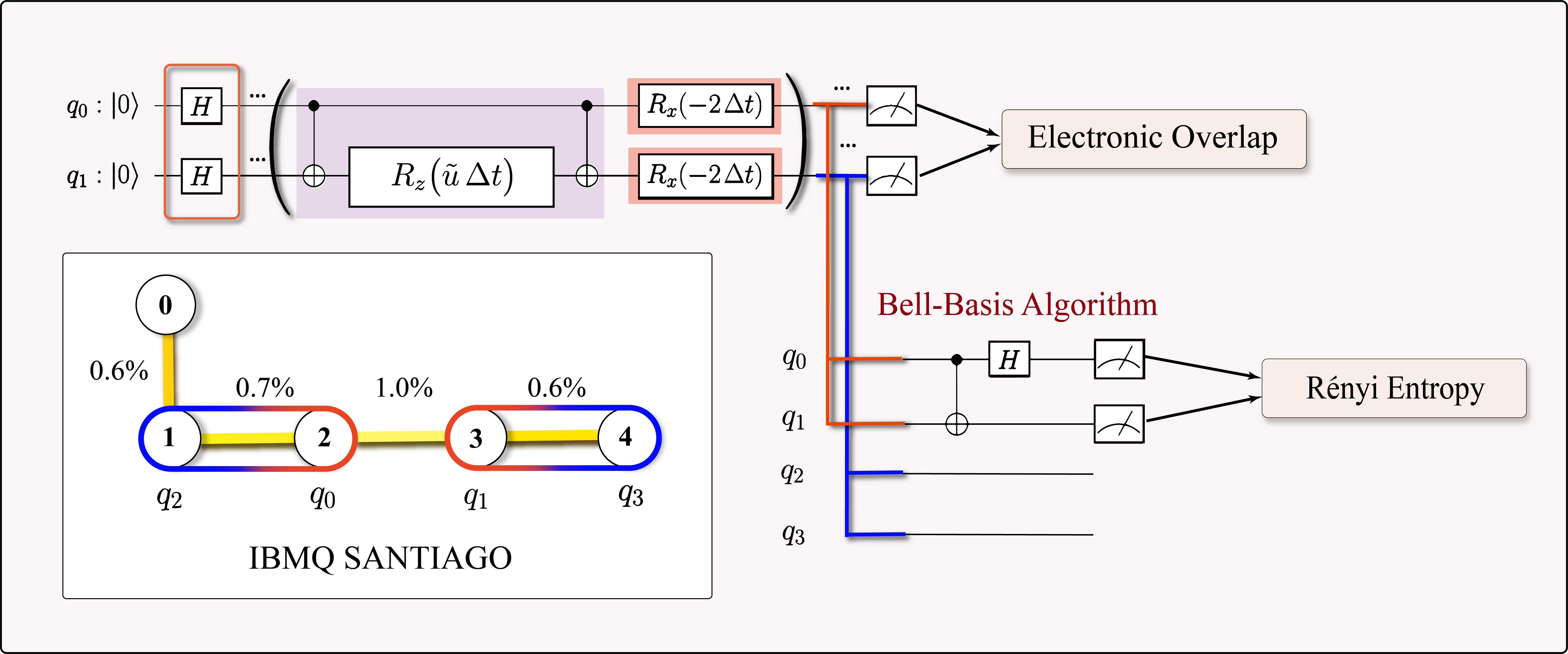
FIG. 5: [Upper Panel] The PFA is used to perform quantum simulation of the Fermi-Hubbard Model. [Lower Right Panel] The Rényi entropy is computed using the Bell-Basis Algorithm.

III.2.2 Computation Parameters

Theoretical Result: To compute the theoretical result, quantum simulation is performed numerically.

The digitization error is estimated by permuting terms in the PFA. Each PFA step contains $3$ unitaries, of which two mutually commute (Figure 5). As such, there are $4^{k}$ total permutations for the $k^{\text{th}}$ PFA step.

III.2.3 Electronic Overlap Dynamics

The presence of electrons occupying shared lattice sites is indicated by the electronic overlap:

$$E_{o}=\Ket{00}\kern-3.00003pt\bra{00}+\Ket{11}\kern-3.00003pt\bra{11}$$ (III.9)

The electronic overlap is measured during quantum simulation of the Fermi-Hubbard Model.

NISQ Computation

QPU Interfacing: The IBMQ-Vigo is accessed via QisKit, which enables preparation of quantum circuits within an intuitive framework [119]. Quantum circuits are packaged into a job object, and sent to the QPU. Each job object can contain up to $75$ individual circuits.

Data Acquisition: The benchmark computation requires $10$ quantum circuits. The circuits are evaluated with a single call to the IBMQ-Vigo. A bootstrap algorithm [120, 121, 122] is run on the measurements to generate the electronic overlap and its uncertainty.

ZNE Noise Mitigation

ZNE is used to establish a performance baseline for CLAWE.

ZNE is performed with a polynomial fit and a Richardson extrapolation.

In both approaches, errors are modulated using the quartic-cycle noise amplification (QCNA) prescription. QCNA amplifies the noise dynamics by injecting pairs of CNOT gates in four rounds of computation (Figure 8). In this work, a ($\times 7$)-QCNA is utilized: ${\mathchoice{\raisebox{0.0pt}{$\displaystyle\chi$}}{\raisebox{0.0pt}{$\textstyle\chi$}}{\raisebox{0.0pt}{$\scriptstyle\chi$}}{\raisebox{0.0pt}{$\scriptscriptstyle\chi$}}}\rightarrow 7\kern 0.90005pt{\mathchoice{\raisebox{0.0pt}{$\displaystyle\chi$}}{\raisebox{0.0pt}{$\textstyle\chi$}}{\raisebox{0.0pt}{$\scriptstyle\chi$}}{\raisebox{0.0pt}{$\scriptscriptstyle\chi$}}}$.

ZNE Viability: ZNE is designed to treat computations that remain within the PNR after error amplification is performed. Applying ($\times 7$)-QCNA to the PFA-expansion probes noise dynamics outside of the PNR (${\mathchoice{\raisebox{0.0pt}{$\displaystyle\chi$}}{\raisebox{0.0pt}{$\textstyle\chi$}}{\raisebox{0.0pt}{$\scriptstyle\chi$}}{\raisebox{0.0pt}{$\scriptscriptstyle\chi$}}}\kern-1.34995pt:20\rightarrow 140$):

$$\text{\small IBMQ-Vigo:}\ {\mathchoice{\raisebox{0.0pt}{$\displaystyle\chi$}}{\raisebox{0.0pt}{$\textstyle\chi$}}{\raisebox{0.0pt}{$\scriptstyle\chi$}}{\raisebox{0.0pt}{$\scriptscriptstyle\chi$}}}_{\text{\tiny PNR}}\approx 111$$ (III.10)

As such, ZNE should reliably correct $7/10$ time-steps.

Polynomial Fit: Performing ZNE with a third-order polynomial fit demonstrates theoretical agreement for $2/10$ points (Figure 8).

Richardson Extrapolation: Performing ZNE with a second-order Richardson extrapolation demonstrates theoretical agreement for $6/10$ points (Figure 8).

CLAWE Noise Mitigation

Variant I and Variant II are applied to the electronic overlap computation.

Variant I: Performing Variant I demonstrates theoretical agreement for $8/10$ points (Figure 15).

Variant II: Performing Variant II demonstrates theoretical agreement for $8/10$ points (Figure 16).

Variant I Calibration: The global noise strength is used to perform extrapolation (Figure 15).

Variant II Calibration: The global noise vector is used to perform extrapolation (Figure 16).

III.2.4 Rényi Entropy Dynamics

The Rényi entropy is measured during quantum simulation of the Fermi-Hubbard Model.

Rényi Entropy

The Hilbert space of the Fermi-Hubbard Model is bipartite in the electron spin:

$$\mathcal{H}=\mathcal{H}_{\uparrow}\otimes\mathcal{H}_{\downarrow}$$ (III.11)

For a state $\rho$, the reduced density matrix for each electron spin species is obtained by applying a partial trace:

$$\rho_{\uparrow}=\text{Tr}_{\downarrow}\big{[}\kern 1.00006pt\rho\kern 1.00006pt\big{]}$$ (III.12)

$$\rho_{\downarrow}=\text{Tr}_{\uparrow}\big{[}\kern 1.00006pt\rho\kern 1.00006pt\big{]}$$ (III.13)

The Rényi entropy of $\rho_{\uparrow}$ is the following:

$$S\kern 0.70007pt(\rho_{\uparrow}) =-\frac{1}{2}\kern 1.00006pt\log{\Big{\{}\kern 1.00006pt\text{Tr}\big{(}\kern 1.00006pt\rho_{\uparrow}^{2}\kern 1.00006pt\big{)}\kern 1.00006pt\Big{\}}}$$ (III.14)

NISQ Computation

The Rényi entropy can be computed using the Bell-Basis Algorithm (BBA) [123].

Bell-Basis Algorithm: Quantum simulation is applied to two copies of the initial state. The quantum stage of the BBA is applied using a CNOT gate between the spin-up qubits (Figure 5).

Data Acquisition: The Rényi entropy computation requires $10$ quantum circuits, which are evaluated with a single call to the IBMQ-Santiago. A bootstrap algorithm is run to generate the Rényi entropy and its uncertainty.

ZNE Noise Mitigation

ZNE is applied to the Rényi entropy computation.

Polynomial Fit: Performing ZNE with a third-order polynomial fit demonstrates theoretical agreement for $1/10$ points (Figure 15).

Richardson Extrapolation: Performing ZNE with a second-order Richardson extrapolation demonstrates theoretical agreement for $4/10$ points (Figure 16).

CLAWE Noise Mitigation

Variant I and Variant II are applied to the Rényi entropy computation.

Variant I: Performing Variant I demonstrates theoretical agreement for $3/10$ points (Figure 15).

Variant II: Performing Variant II demonstrates theoretical agreement for $7/10$ points (Figure 16).

IV Acknowledgements

The author is supported in part by the Maryland Center for Fundamental Physics, University of Maryland, College Park and by the U.S. Department of Energy (DOE), Office of Science, Office of Advanced Scientific Computing Research (ASCR) Quantum Computing Applications Teams program, under fieldwork proposal number ERKJ347.

 

Those who wait on the Lord shall renew their strength; they shall mount up with wings like eagles, they shall run and not be weary, they shall walk and not faint.

-Isaiah 40:31

$-AMDG-$

Appendix

I Noise Tailoring Algorithms

Coarse-grained decoupling [124, 125, 126, 127] can be used to alter noise dynamics using gate-level control. Oliver Kern, Gernot Alber, and Dima Shepelyansky first demonstrated this using Pauli Random Error Correction (PAREC) [124].

In PAREC, the computational frame is toggled during a computation by inserting randomized pairs of Pauli operations. This leaves the computation logically equivalent. Toggling the computational frame generates a dynamical decoupling-like effect without the need for rapid time-modulation [128].

The NT algorithm used in this work is Randomized Compiling (RCo) [126]. RCo applies coarse-grained decoupling across a sequence of circuits.

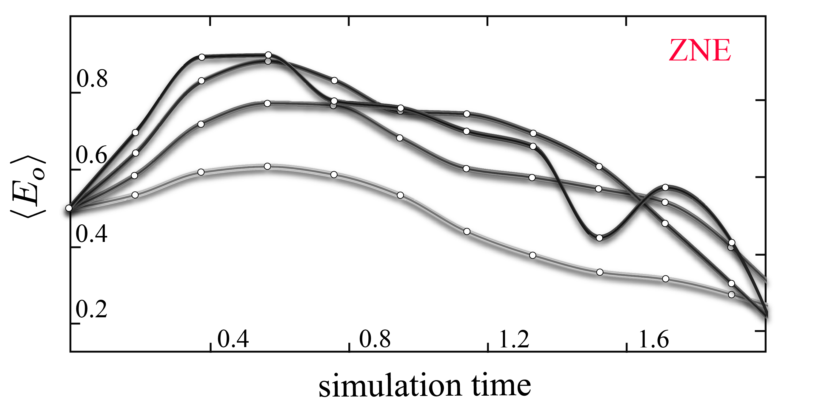
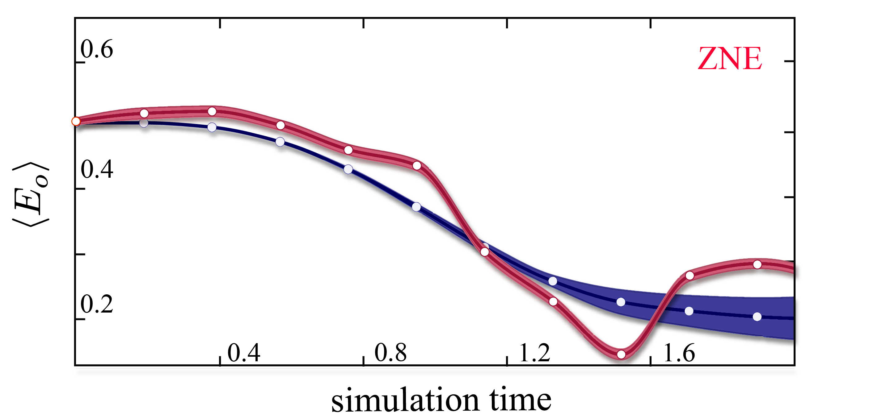
FIG. 6: Error-amplified dynamics (gray), are extrapolated to the zero-noise solution.

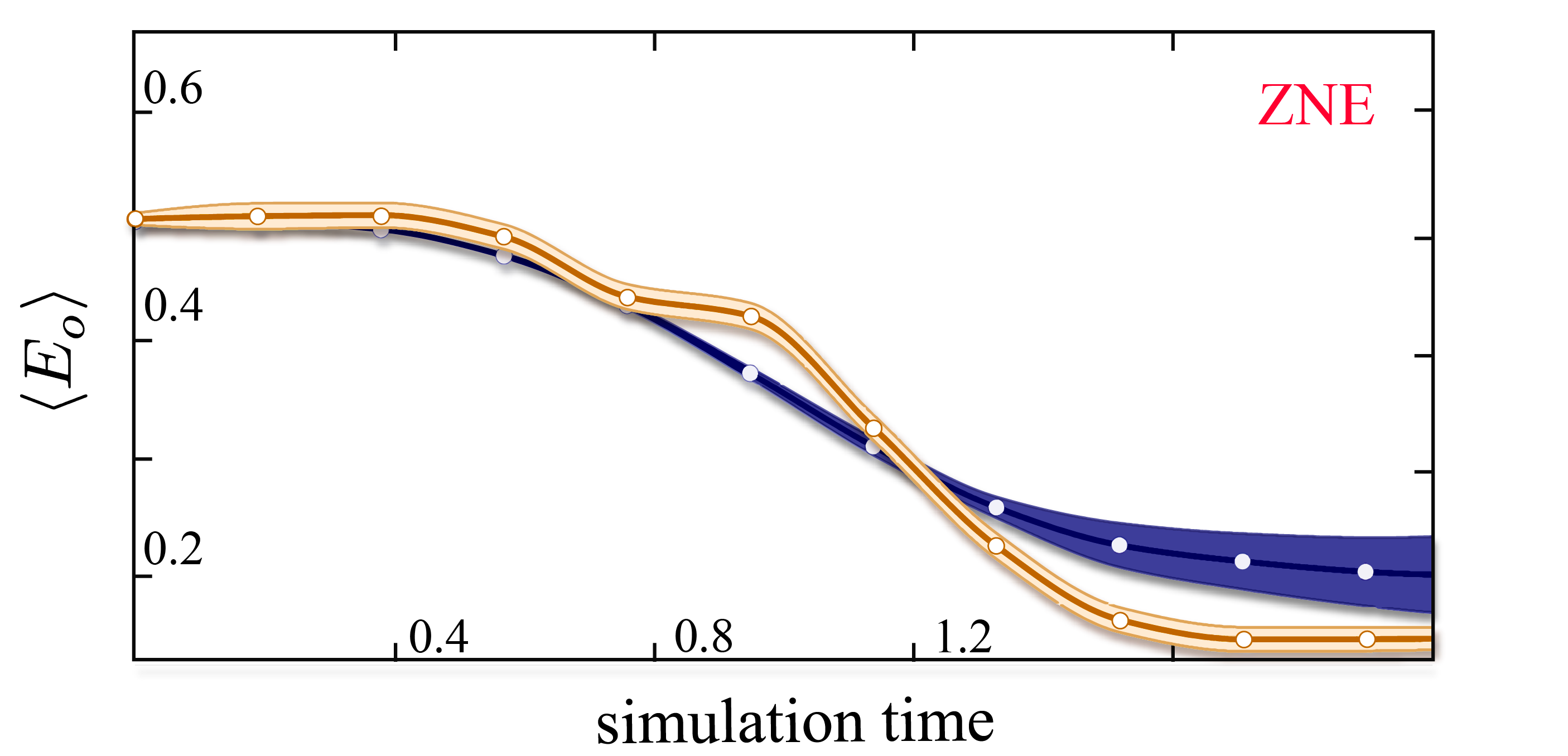
FIG. 7: The ZNE polynomial fit (red) is compared with the theoretical result (indigo) for the electronic overlap.

FIG. 8: The ZNE Richardson extrapolation (golden) is compared with the theoretical result (indigo) for the electronic overlap.

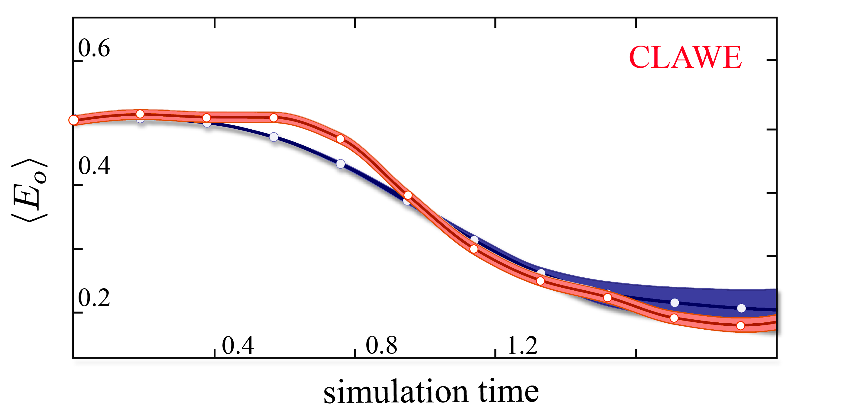
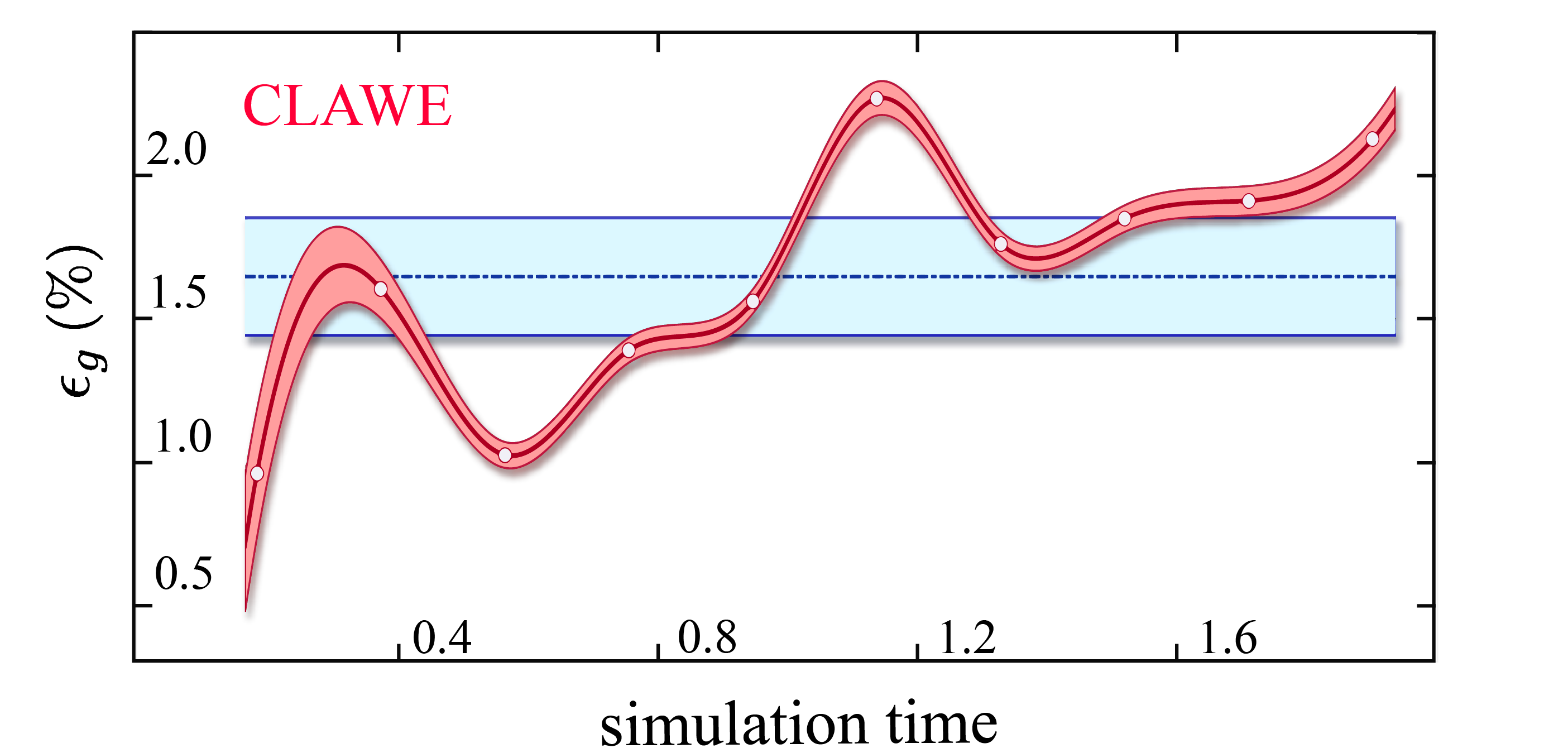
FIG. 9: Variant I (red) is compared with the theoretical result (indigo) for the electronic overlap.

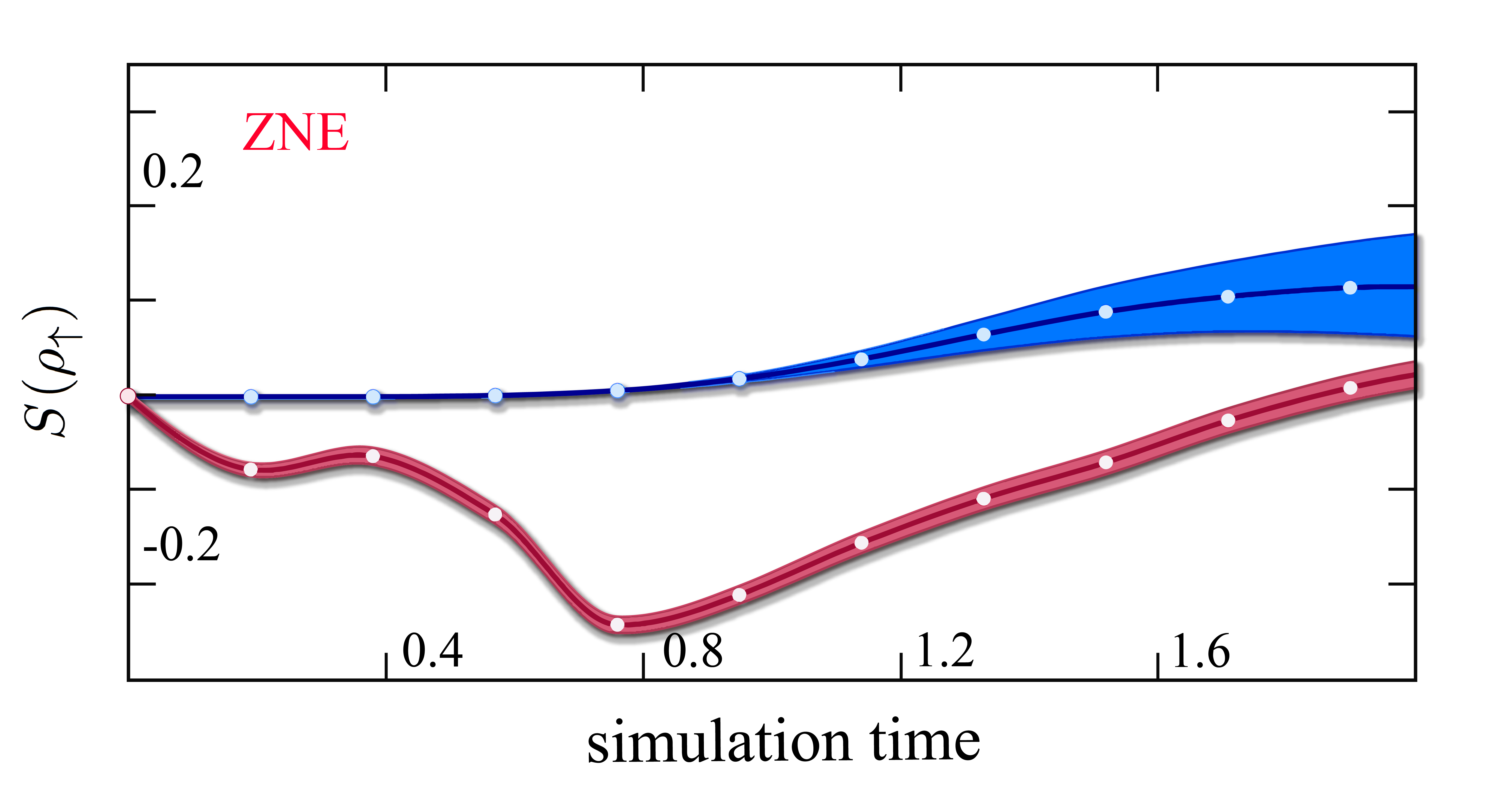
FIG. 11: The global noise strength (red) is shown alongside its mean value (blue).

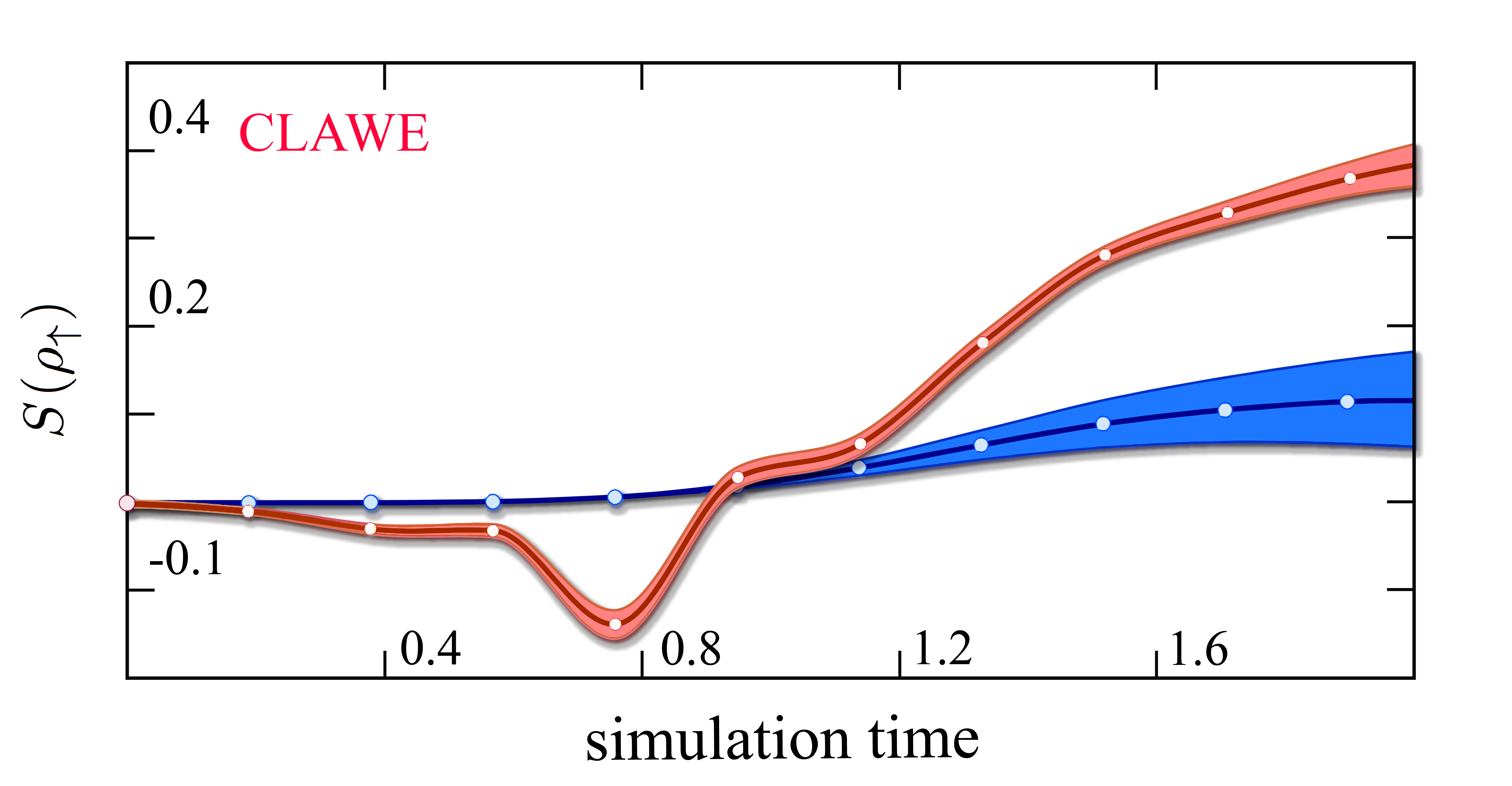
FIG. 13: The ZNE polynomial fit (red) is compared with the theoretical result (blue) for the Rényi entropy.

FIG. 15: Variant I (red) is compared with the theoretical result (blue) for the Rényi entropy.

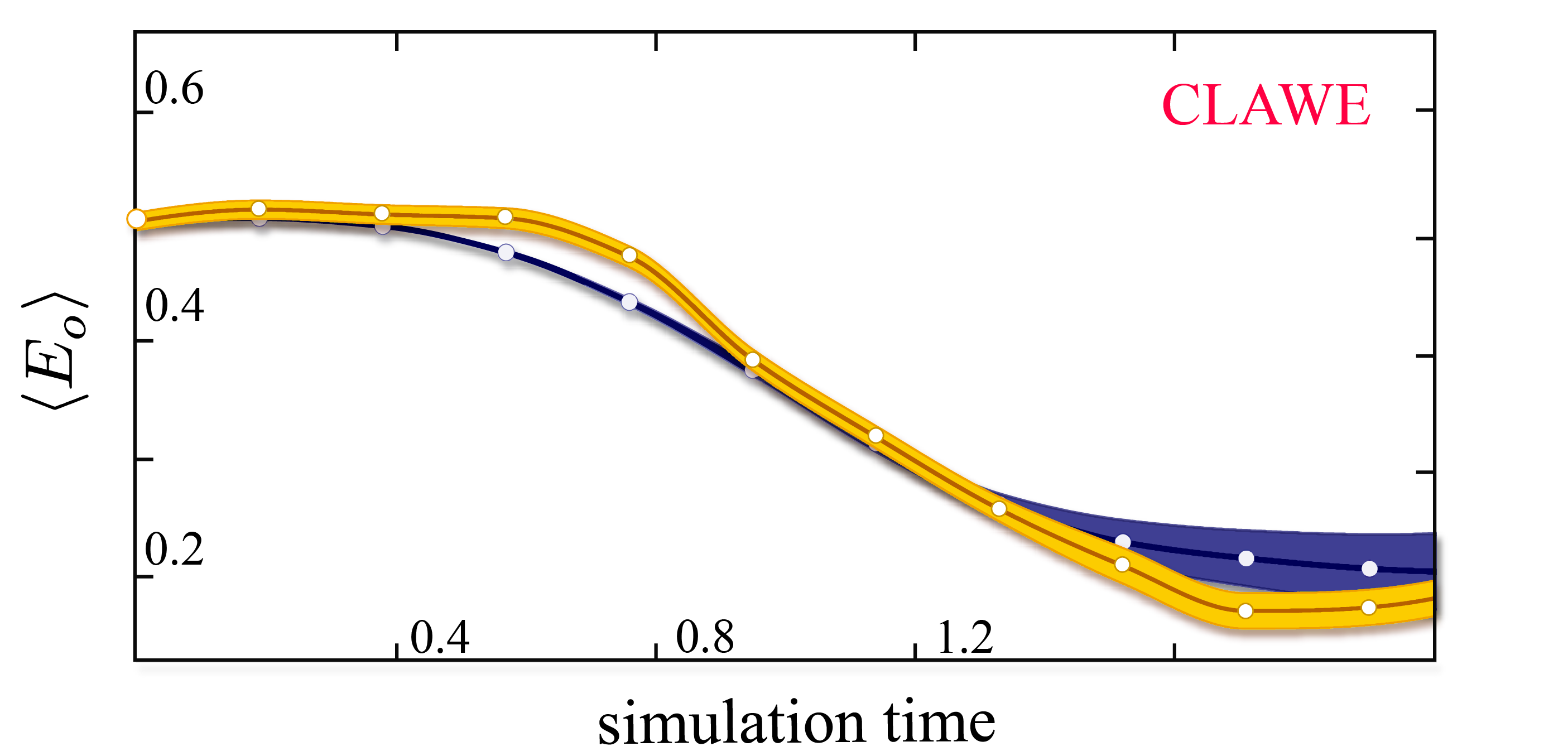
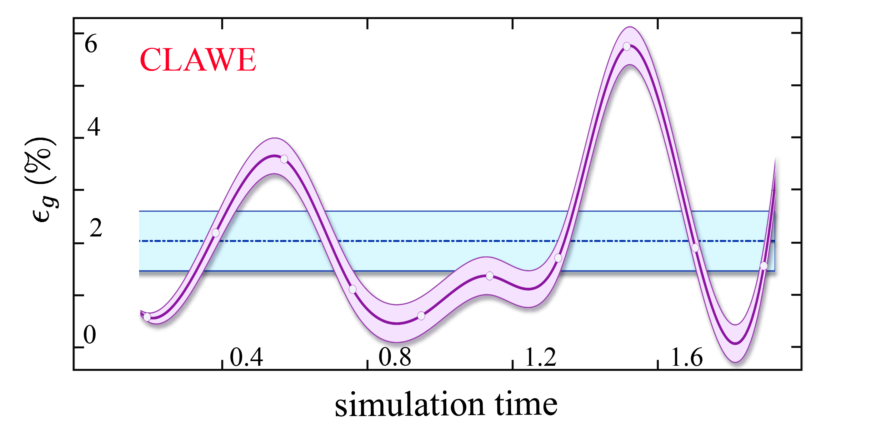
FIG. 10: Variant II (golden) is compared with the theoretical result (indigo) for the electronic overlap.

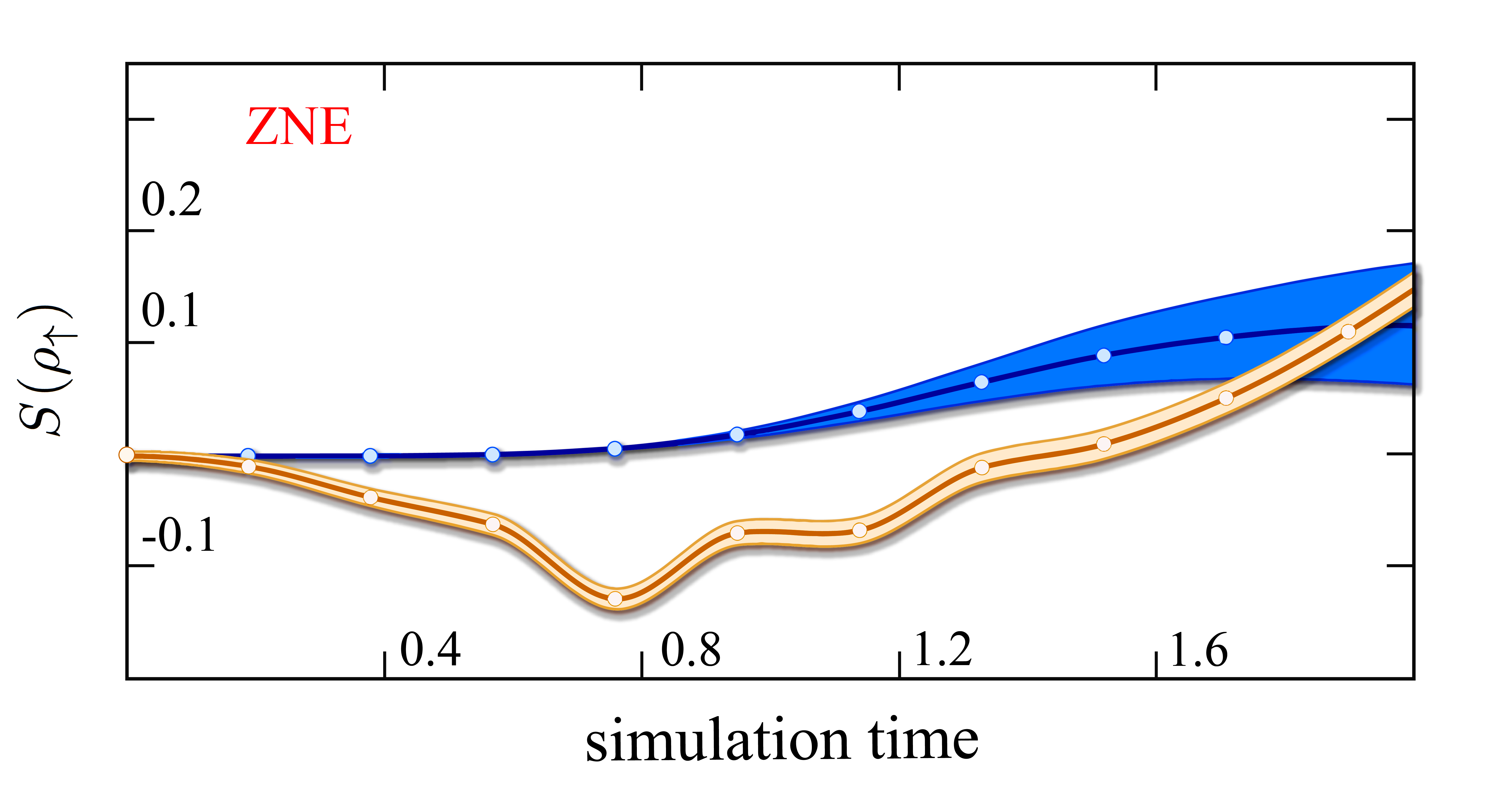
FIG. 12: The global noise vector (purple) is shown alongside its mean value (blue).

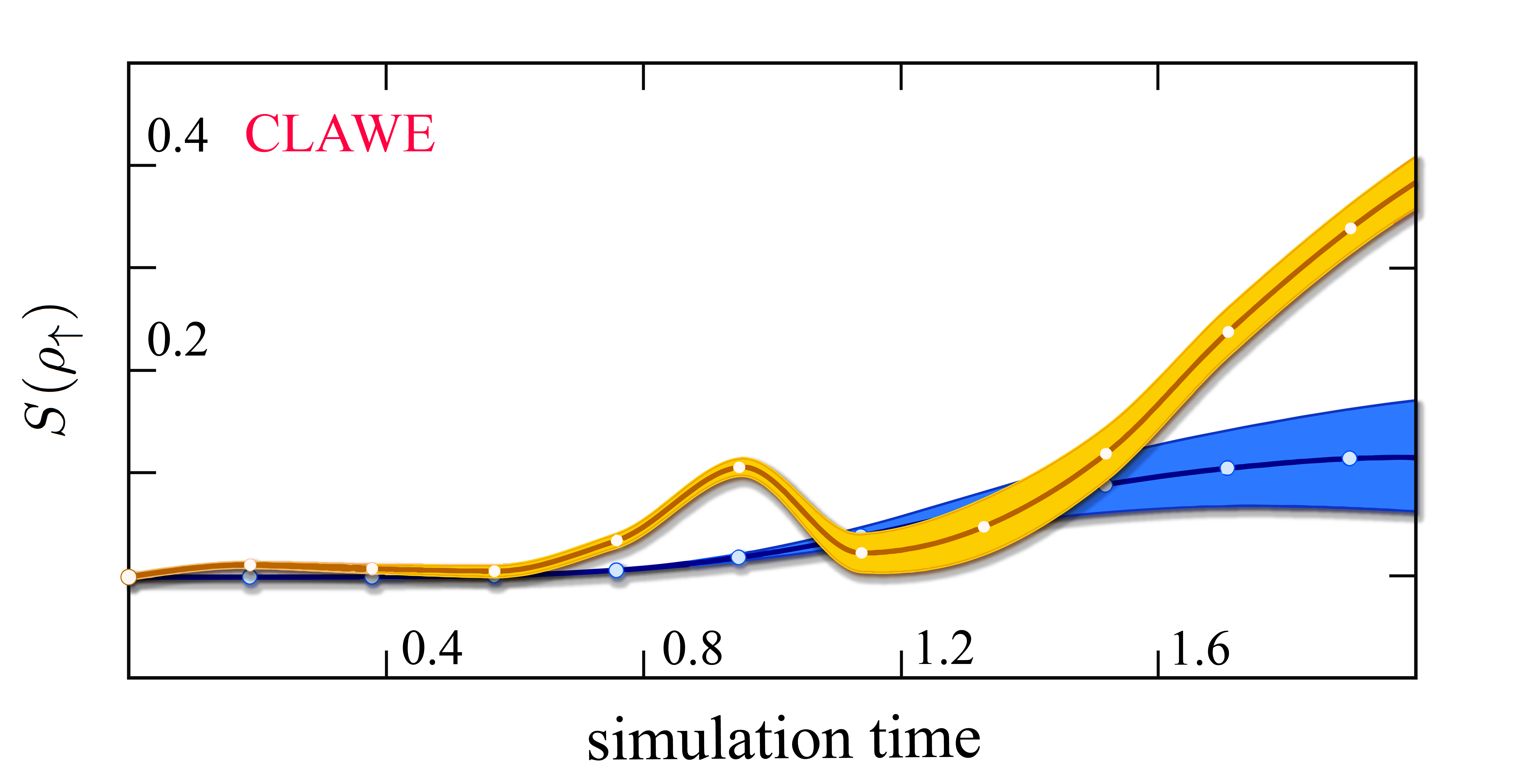
FIG. 14: The ZNE Richardson extrapolation (golden) is compared with the theoretical result (blue) for the Rényi entropy.

FIG. 16: Variant II (golden) is compared with the theoretical result (blue) for the Rényi entropy.

References

- Abrams et al. [2019] D. M. Abrams, N. Didier, S. A. Caldwell, B. R. Johnson, and C. A. Ryan, Methods for measuring magnetic flux crosstalk between tunable transmons, Phys. Rev. Applied 12, 064022 (2019).
- Hashim et al. [2020] A. Hashim, R. K. Naik, A. Morvan, J.-L. Ville, B. Mitchell, J. M. Kreikebaum, M. Davis, E. Smith, C. Iancu, K. P. O’Brien, I. Hincks, J. J. Wallman, J. Emerson, and I. Siddiqi, Randomized compiling for scalable quantum computing on a noisy superconducting quantum processor, (2020), arXiv:2010.00215 [quant-ph] .
- Ding et al. [2020] Y. Ding, P. Gokhale, S. Fuhui Lin, R. Rines, T. Propson, and F. T. Chong, Systematic Crosstalk Mitigation for Superconducting Qubits via Frequency-Aware Compilation, arXiv e-prints , arXiv:2008.09503 (2020), arXiv:2008.09503 [quant-ph] .
- Yousefjani and Bayat [2020] R. Yousefjani and A. Bayat, Parallel entangling gate operations and two-way quantum communication in spin chains, (2020), arXiv:2008.12771 [quant-ph] .
- Willsch [2020] D. Willsch, Supercomputer simulations of transmon quantum computers, arXiv e-prints , arXiv:2008.13490 (2020), arXiv:2008.13490 [quant-ph] .
- Winick et al. [2020] A. Winick, J. J. Wallman, and J. Emerson, Simulating and mitigating crosstalk, (2020), arXiv:2006.09596 [quant-ph] .
- Xu et al. [2020] Y. Xu, J. Chu, J. Yuan, J. Qiu, Y. Zhou, L. Zhang, X. Tan, Y. Yu, S. Liu, J. Li, F. Yan, and D. Yu, High-fidelity, high-scalability two-qubit gate scheme for superconducting qubits, (2020), arXiv:2006.11860 [quant-ph] .
- Collodo et al. [2020] M. C. Collodo, J. Herrmann, N. Lacroix, C. K. Andersen, A. Remm, S. Lazar, J.-C. Besse, T. Walter, A. Wallraff, and C. Eichler, Implementation of Conditional-Phase Gates based on tunable ZZ-Interactions (2020), arXiv:2005.08863 [quant-ph] .
- Krinner et al. [2020] S. Krinner, S. Lazar, A. Remm, C. Andersen, N. Lacroix, G. Norris, C. Hellings, M. Gabureac, C. Eichler, and A. Wallraff, Benchmarking coherent errors in controlled-phase gates due to spectator qubits, Phys. Rev. Applied 14, 024042 (2020).
- Throckmorton and Das Sarma [2020] R. E. Throckmorton and S. Das Sarma, Fidelity of a sequence of swap operations on a spin chain, Phys. Rev. B 102, 035439 (2020).
- McKay et al. [2020] D. C. McKay, A. W. Cross, C. J. Wood, and J. M. Gambetta, Correlated Randomized Benchmarking, (2020), arXiv:2003.02354 [quant-ph] .
- Ku et al. [2020] J. Ku, X. Xu, M. Brink, D. C. McKay, J. B. Hertzberg, M. H. Ansari, and B. L. T. Plourde, Suppression of Unwanted Interactions in a Hybrid Two-Qubit System, (2020), arXiv:2003.02775 [quant-ph] .
- Han et al. [2020] X. Y. Han, T. Q. Cai, X. G. Li, Y. K. Wu, Y. W. Ma, Y. L. Ma, J. H. Wang, H. Y. Zhang, Y. P. Song, and L. M. Duan, Error analysis in suppression of unwanted qubit interactions for a parametric gate in a tunable superconducting circuit, Phys. Rev. A 102, 022619 (2020).
- Huang et al. [2020] C. Huang, X. Ni, F. Zhang, M. Newman, D. Ding, X. Gao, T. Wang, H.-H. Zhao, F. Wu, G. Zhang, C. Deng, H.-S. Ku, J. Chen, and Y. Shi, Alibaba Cloud Quantum Development Platform: Surface Code Simulations with Crosstalk, (2020), arXiv:2002.08918 [quant-ph] .
- Kono et al. [2020] S. Kono, K. Koshino, D. Lachance-Quirion, A. F. van Loo, Y. Tabuchi, A. Noguchi, and Y. Nakamura, Breaking the trade-off between fast control and long lifetime of a superconducting qubit, Nature Communications 11, 3683 (2020).
- Murali et al. [2020] P. Murali, D. C. Mckay, M. Martonosi, and A. Javadi-Abhari, Software mitigation of crosstalk on noisy intermediate-scale quantum computers 10.1145/3373376.3378477 (2020).
- Sun et al. [2020] J. Sun, X. Yuan, T. Tsunoda, V. Vedral, S. C. Bejamin, and S. Endo, Mitigating realistic noise in practical noisy intermediate-scale quantum devices, (2020), arXiv:2001.04891 [quant-ph] .
- Güngördü and Kestner [2020] U. Güngördü and J. P. Kestner, Robust implementation of quantum gates despite always-on exchange coupling in silicon double quantum dots, Phys. Rev. B 101, 155301 (2020).
- Qi and Jing [2020] S.-f. Qi and J. Jing, Generating noon states in circuit qed using a multiphoton resonance in the presence of counter-rotating interactions, Phys. Rev. A 101, 033809 (2020).
- Debroy et al. [2020] D. M. Debroy, M. Li, S. Huang, and K. R. Brown, Logical Performance of 9 Qubit Compass Codes in Ion Traps with Crosstalk Errors, (2020), arXiv:1910.08495 [quant-ph] .
- Sarovar et al. [2020] M. Sarovar, T. Proctor, K. Rudinger, K. Young, E. Nielsen, and R. Blume-Kohout, Detecting crosstalk errors in quantum information processors, Quantum 4, 321 (2020).
- Chamberland et al. [2020] C. Chamberland, G. Zhu, T. J. Yoder, J. B. Hertzberg, and A. W. Cross, Topological and subsystem codes on low-degree graphs with flag qubits, Phys. Rev. X 10, 011022 (2020).
- Majumder et al. [2020] S. Majumder, L. Andreta de Castro, and K. R. Brown, Real-time calibration with spectator qubits, npj Quantum Information 6, 19 (2020).
- Harper et al. [2020] R. Harper, S. T. Flammia, and J. J. Wallman, Efficient learning of quantum noise, Nature Physics 10.1038/s41567-020-0992-8 (2020).
- Ash-Saki et al. [2020] A. Ash-Saki, M. Alam, and S. Ghosh, Analysis of crosstalk in nisq devices and security implications in multi-programming regime, , 25 (2020).
- Shaw [2019a] A. Shaw, A New Noise Mitigation Scheme for Computations on NISQ-era Devices (June 19, 2019a), UMD NISQ/TQC Conference.
- Shaw [2019b] A. Shaw, Extending the Range of Near-Term Quantum Simulation with Classical-Quantum Hybrid Methods (October 13, 2019b), Fall 2019 DNP-APS Meeting.
- Shaw [2019c] A. Shaw, A Noise Mitigation Scheme for NISQ Hardware (December 04, 2019c), FAR-QC Conference.
- Shaw [2020a] A. Shaw, Classical-Quantum Noise Mitigation for NISQ Devices (June 23, 2020a), Quantum Computing Applications Team Meeting.
- Paraoanu [2006] G. S. Paraoanu, Microwave-induced coupling of superconducting qubits, Phys. Rev. B 74, 140504 (2006).
- Li et al. [2008] J. Li, K. Chalapat, and G. S. Paraoanu, Entanglement of superconducting qubits via microwave fields: Classical and quantum regimes, Phys. Rev. B 78, 064503 (2008).
- Li et al. [2009] J. Li, K. Chalapat, and G. S. Paraoanu, Measurement-induced entanglement of two superconducting qubits, Journal of Physics: Conference Series 150, 022051 (2009).
- Kurpas et al. [2009] M. Kurpas, J. Dajka, and E. Zipper, Entanglement of qubits via a nonlinear resonator, Journal of Physics: Condensed Matter 21, 235602 (2009).
- Li and Paraoanu [2009] J. Li and G. S. Paraoanu, Generation and propagation of entanglement in driven coupled-qubit systems, New Journal of Physics 11, 113020 (2009).
- Rigetti and Devoret [2010] C. Rigetti and M. Devoret, Fully microwave-tunable universal gates in superconducting qubits with linear couplings and fixed transition frequencies, Phys. Rev. B 81, 134507 (2010).
- [36] J. F. Leandro, A. S. M. de Castro, P. P. Munhoz, and F. L. Semião, Active control of qubit-qubit entanglement evolution, Physics Letters A , 4199.
- Chow et al. [2011] J. M. Chow, A. D. Córcoles, J. M. Gambetta, C. Rigetti, B. R. Johnson, J. A. Smolin, J. R. Rozen, G. A. Keefe, M. B. Rothwell, M. B. Ketchen, and M. Steffen, Simple all-microwave entangling gate for fixed-frequency superconducting qubits, Phys. Rev. Lett. 107, 080502 (2011).
- Chaudhry and Gong [2012] A. Z. Chaudhry and J. Gong, Decoherence control: Universal protection of two-qubit states and two-qubit gates using continuous driving fields, Phys. Rev. A 85, 012315 (2012).
- Lü et al. [2012] X.-Y. Lü, S. Ashhab, W. Cui, R. Wu, and F. Nori, Two-qubit gate operations in superconducting circuits with strong coupling and weak anharmonicity, New Journal of Physics 14, 073041 (2012).
- de Groot et al. [2012] P. C. de Groot, S. Ashhab, A. Lupaşcu, L. DiCarlo, F. Nori, C. J. P. M. Harmans, and J. E. Mooij, Selective darkening of degenerate transitions for implementing quantum controlled-NOT gates, New Journal of Physics 14, 073038 (2012).
- Chow et al. [2012] J. M. Chow, J. M. Gambetta, A. D. Córcoles, S. T. Merkel, J. A. Smolin, C. Rigetti, S. Poletto, G. A. Keefe, M. B. Rothwell, J. R. Rozen, M. B. Ketchen, and M. Steffen, Universal quantum gate set approaching fault-tolerant thresholds with superconducting qubits, Phys. Rev. Lett. 109, 060501 (2012).
- Poletto et al. [2012] S. Poletto, J. M. Gambetta, S. T. Merkel, J. A. Smolin, J. M. Chow, A. D. Córcoles, G. A. Keefe, M. B. Rothwell, J. R. Rozen, D. W. Abraham, C. Rigetti, and M. Steffen, Entanglement of two superconducting qubits in a waveguide cavity via monochromatic two-photon excitation, Phys. Rev. Lett. 109, 240505 (2012).
- Ghosh et al. [2013] J. Ghosh, A. Galiautdinov, Z. Zhou, A. N. Korotkov, J. M. Martinis, and M. R. Geller, High-fidelity controlled- gate for resonator-based superconducting quantum computers, Phys. Rev. A 87, 022309 (2013).
- Córcoles et al. [2013] A. D. Córcoles, J. M. Gambetta, J. M. Chow, J. A. Smolin, M. Ware, J. Strand, B. L. T. Plourde, and M. Steffen, Process verification of two-qubit quantum gates by randomized benchmarking, Phys. Rev. A 87, 030301 (2013).
- Leghtas et al. [2013] Z. Leghtas, U. Vool, S. Shankar, M. Hatridge, S. M. Girvin, M. H. Devoret, and M. Mirrahimi, Stabilizing a bell state of two superconducting qubits by dissipation engineering, Phys. Rev. A 88, 023849 (2013).
- Reiter et al. [2013] F. Reiter, L. Tornberg, G. Johansson, and A. S. Sørensen, Steady-state entanglement of two superconducting qubits engineered by dissipation, Phys. Rev. A 88, 032317 (2013).
- Egger and Wilhelm [2013] D. J. Egger and F. K. Wilhelm, Optimized controlled-z gates for two superconducting qubits coupled through a resonator, Superconductor Science and Technology 27, 014001 (2013).
- Huang and Goan [2014] S.-Y. Huang and H.-S. Goan, Optimal control for fast and high-fidelity quantum gates in coupled superconducting flux qubits, Phys. Rev. A 90, 012318 (2014).
- Chakhmakhchyan et al. [2014] L. Chakhmakhchyan, C. Leroy, N. Ananikian, and S. Guérin, Generation of entanglement in systems of intercoupled qubits, Phys. Rev. A 90, 042324 (2014).
- Yang et al. [2016] C.-P. Yang, Q.-P. Su, S.-B. Zheng, and F. Nori, Entangling superconducting qubits in a multi-cavity system, New Journal of Physics 18, 013025 (2016).
- Kirchhoff et al. [2018] S. Kirchhoff, T. Keßler, P. J. Liebermann, E. Assémat, S. Machnes, F. Motzoi, and F. K. Wilhelm, Optimized cross-resonance gate for coupled transmon systems, Phys. Rev. A 97, 042348 (2018).
- Qi et al. [2018] Z. Qi, H.-Y. Xie, J. Shabani, V. E. Manucharyan, A. Levchenko, and M. G. Vavilov, Controlled-z gate for transmon qubits coupled by semiconductor junctions, Phys. Rev. B 97, 134518 (2018).
- Noh et al. [2018] T. Noh, G. Park, S.-G. Lee, W. Song, and Y. Chong, Construction of controlled-not gate based on microwave-activated phase (map) gate in two transmon system, Scientific Reports 8, 13598 (2018).
- Nesterov et al. [2018] K. N. Nesterov, I. V. Pechenezhskiy, C. Wang, V. E. Manucharyan, and M. G. Vavilov, Microwave-activated controlled- gate for fixed-frequency fluxonium qubits, Phys. Rev. A 98, 030301 (2018).
- Caldwell et al. [2018] S. A. Caldwell, N. Didier, C. A. Ryan, E. A. Sete, A. Hudson, P. Karalekas, R. Manenti, M. P. da Silva, R. Sinclair, E. Acala, N. Alidoust, J. Angeles, A. Bestwick, M. Block, B. Bloom, A. Bradley, C. Bui, L. Capelluto, R. Chilcott, J. Cordova, G. Crossman, M. Curtis, S. Deshpande, T. E. Bouayadi, D. Girshovich, S. Hong, K. Kuang, M. Lenihan, T. Manning, A. Marchenkov, J. Marshall, R. Maydra, Y. Mohan, W. O’Brien, C. Osborn, J. Otterbach, A. Papageorge, J.-P. Paquette, M. Pelstring, A. Polloreno, G. Prawiroatmodjo, V. Rawat, M. Reagor, R. Renzas, N. Rubin, D. Russell, M. Rust, D. Scarabelli, M. Scheer, M. Selvanayagam, R. Smith, A. Staley, M. Suska, N. Tezak, D. C. Thompson, T.-W. To, M. Vahidpour, N. Vodrahalli, T. Whyland, K. Yadav, W. Zeng, and C. Rigetti, Parametrically activated entangling gates using transmon qubits, Phys. Rev. Applied 10, 034050 (2018).
- Yan et al. [2018] F. Yan, P. Krantz, Y. Sung, M. Kjaergaard, D. L. Campbell, T. P. Orlando, S. Gustavsson, and W. D. Oliver, Tunable coupling scheme for implementing high-fidelity two-qubit gates, Phys. Rev. Applied 10, 054062 (2018).
- Premaratne et al. [2019] S. P. Premaratne, J.-H. Yeh, F. C. Wellstood, and B. S. Palmer, Implementation of a generalized controlled-not gate between fixed-frequency transmons, Phys. Rev. A 99, 012317 (2019).
- Rasmussen et al. [2019] S. E. Rasmussen, K. S. Christensen, and N. T. Zinner, Controllable two-qubit swapping gate using superconducting circuits, Phys. Rev. B 99, 134508 (2019).
- Tripathi et al. [2019] V. Tripathi, M. Khezri, and A. N. Korotkov, Operation and intrinsic error budget of a two-qubit cross-resonance gate, Phys. Rev. A 100, 012301 (2019).
- Patterson et al. [2019] A. Patterson, J. Rahamim, T. Tsunoda, P. Spring, S. Jebari, K. Ratter, M. Mergenthaler, G. Tancredi, B. Vlastakis, M. Esposito, and P. Leek, Calibration of a cross-resonance two-qubit gate between directly coupled transmons, Phys. Rev. Applied 12, 064013 (2019).
- Hong et al. [2020] S. S. Hong, A. T. Papageorge, P. Sivarajah, G. Crossman, N. Didier, A. M. Polloreno, E. A. Sete, S. W. Turkowski, M. P. da Silva, and B. R. Johnson, Demonstration of a parametrically activated entangling gate protected from flux noise, Phys. Rev. A 101, 012302 (2020).
- Barron et al. [2020] G. S. Barron, F. A. Calderon-Vargas, J. Long, D. P. Pappas, and S. E. Economou, Microwave-based arbitrary cphase gates for transmon qubits, Phys. Rev. B 101, 054508 (2020).
- Loft et al. [2020] N. J. S. Loft, M. Kjaergaard, L. B. Kristensen, C. K. Andersen, T. W. Larsen, S. Gustavsson, W. D. Oliver, and N. T. Zinner, Quantum interference device for controlled two-qubit operations, npj Quantum Information 6, 47 (2020).
- Rasmussen and Zinner [2020] S. E. Rasmussen and N. T. Zinner, Simple implementation of high fidelity controlled-swap gates and quantum circuit exponentiation of non-hermitian gates, Phys. Rev. Research 2, 033097 (2020).
- Zhang et al. [2020] C.-L. Zhang, W.-W. Liu, and X.-M. Lin, One-step implementation of a robust fredkin gate based on path engineering, Quantum Information Processing 19, 265 (2020).
- Ganzhorn et al. [2020] M. Ganzhorn, G. Salis, D. J. Egger, A. Fuhrer, M. Mergenthaler, C. Müller, P. Müller, S. Paredes, M. Pechal, M. Werninghaus, and S. Filipp, Benchmarking the noise sensitivity of different parametric two-qubit gates in a single superconducting quantum computing platform, Phys. Rev. Research 2, 033447 (2020).
- Fano [1995] U. Fano, Matrici di densità come vettori di polarizzazione, Rendiconti Lincei 6, 123 (1995).
- den [1965] 2 - the damping problem in wave mechanics, in Collected Papers of L.D. Landau, edited by D. T. HAAR (Pergamon, 1965) pp. 8 – 18.
- Neumann [1927] J. v. Neumann, Wahrscheinlichkeitstheoretischer aufbau der quantenmechanik, Nachrichten von der Gesellschaft der Wissenschaften zu Göttingen, Mathematisch-Physikalische Klasse 1927, 245 (1927).
- Choi [1975] M.-D. Choi, Completely positive linear maps on complex matrices, Linear Algebra and its Applications 10, 285 (1975).
- Weedbrook et al. [2012] C. Weedbrook, S. Pirandola, R. García-Patrón, N. J. Cerf, T. C. Ralph, J. H. Shapiro, and S. Lloyd, Gaussian quantum information, Rev. Mod. Phys. 84, 621 (2012).
- Novikov [1970] I. D. Novikov, Gibbs state in quantum statistical physics, Functional Analysis and Its Applications 4, 334 (1970).
- Ticozzi and Viola [2017] F. Ticozzi and L. Viola, Quantum and classical resources for unitary design of open-system evolutions, Quantum Science and Technology 2, 034001 (2017).
- Stinespring [1955] W. F. Stinespring, Positive functions on c*-algebras, Proceedings of the American Mathematical Society 6, 211 (1955).
- Nielsen [2002] M. A. Nielsen, A simple formula for the average gate fidelity of a quantum dynamical operation, Physics Letters A 303, 249 (2002).
- Sobiczewski and Litvinov [2014] A. Sobiczewski and Y. A. Litvinov, Predictive power of nuclear-mass models, Phys. Rev. C 90, 017302 (2014).
- Neufcourt et al. [2018] L. Neufcourt, Y. Cao, W. Nazarewicz, and F. Viens, Bayesian approach to model-based extrapolation of nuclear observables, Phys. Rev. C 98, 034318 (2018).
- Negoita et al. [2019] G. A. Negoita, J. P. Vary, G. R. Luecke, P. Maris, A. M. Shirokov, I. J. Shin, Y. Kim, E. G. Ng, C. Yang, M. Lockner, and G. M. Prabhu, Deep learning: Extrapolation tool for ab initio nuclear theory, Phys. Rev. C 99, 054308 (2019).
- Jiang et al. [2019] W. G. Jiang, G. Hagen, and T. Papenbrock, Extrapolation of nuclear structure observables with artificial neural networks, Phys. Rev. C 100, 054326 (2019).
- Temme et al. [2017] K. Temme, S. Bravyi, and J. M. Gambetta, Error mitigation for short-depth quantum circuits, Phys. Rev. Lett. 119, 180509 (2017).
- Li and Benjamin [2017] Y. Li and S. C. Benjamin, Efficient variational quantum simulator incorporating active error minimization, Phys. Rev. X 7, 021050 (2017).
- Shaw [2020b] A. Shaw, Benchmarking Non-Abelian Lattice Gauge Theories With NISQ Algorithms (October 31, 2020b), 2020 Fall Meeting of the APS Division of Nuclear Physics.
- Yamada [1962] H. Yamada, Real-time computation and recursive functions not real-time computable, IRE Transactions on Electronic Computers EC-11, 753 (1962).
- Smale [1997] S. Smale, Complexity theory and numerical analysis, Acta Numerica 6, 523–551 (1997).
- Aaronson [2013] S. J. Aaronson, Quantum Computing Since Democritus (Cambridge University Press, USA, 2013) Chap. 5, pp. 44–50.
- Scott et al. [2020] A. Scott, G. Kuperberg, and C. Granade, Complexity zoo, February 18 (2020).
- Cobham [1965] A. Cobham, Logic, Methodology and Philosophy of Science: Proceedings of the 1964 International Congress (North-Holland Publishing, 1965) Chap. The Intrinsic Computational Difficulty of Functions, pp. 24–30.
- Edmonds [1965] J. Edmonds, Paths, trees, and flowers, Canadian Journal of Mathematics 17, 449 (1965).
- Goldreich [2008] O. Goldreich, Computational complexity. A conceptual perspective, Vol. 39 (2008) pp. 32–33.
- Turing [1937] A. M. Turing, On computable numbers, with an application to the entscheidungsproblem, Proceedings of the London Mathematical Society s2-42, 230 (1937).
- Turing [1938] A. M. Turing, On computable numbers, with an application to the entscheidungsproblem. a correction, Proceedings of the London Mathematical Society s2-43, 544 (1938).
- Turing [1996] A. M. Turing, Intelligent Machinery, A Heretical Theory*, Philosophia Mathematica 4, 256 (1996).
- Benioff [1980] P. Benioff, The computer as a physical system: A microscopic quantum mechanical hamiltonian model of computers as represented by turing machines, Journal of Statistical Physics 22, 563 (1980).
- Benioff [1982] P. Benioff, Quantum mechanical hamiltonian models of turing machines, Journal of Statistical Physics 29, 515 (1982).
- Deutsch and Penrose [1985] D. Deutsch and R. Penrose, Quantum theory, the church-turing principle and the universal quantum computer, Proceedings of the Royal Society of London. A. Mathematical and Physical Sciences 400, 97 (1985).
- Sipser [2012] M. Sipser, Introduction to the Theory of Computation (Cengage Learning, 2012).
- Bernstein and Vazirani [1997] E. Bernstein and U. Vazirani, Quantum complexity theory, SIAM Journal on Computing 26, 1411 (1997).
- Aaronson and Ben-David [2015] S. Aaronson and S. Ben-David, Sculpting Quantum Speedups, arXiv e-prints , arXiv:1512.04016 (2015), arXiv:1512.04016 [quant-ph] .
- Feynman [1982] R. P. Feynman, Simulating physics with computers, International Journal of Theoretical Physics 21, 467 (1982).
- Lloyd [1996] S. Lloyd, Universal quantum simulators, Science 273, 1073 (1996).
- Aharonov and Ta-Shma [2003] D. Aharonov and A. Ta-Shma, Adiabatic quantum state generation and statistical zero knowledge, in Proceedings of the Thirty-Fifth Annual ACM Symposium on Theory of Computing (Association for Computing Machinery, New York, NY, USA, 2003) pp. 20–29.
- Nagaj [2010] D. Nagaj, Fast universal quantum computation with railroad-switch local Hamiltonians, Journal of Mathematical Physics 51, 062201 (2010), arXiv:0908.4219 [quant-ph] .
- Berry et al. [2015] D. W. Berry, A. M. Childs, and R. Kothari, Hamiltonian simulation with nearly optimal dependence on all parameters, arXiv e-prints , arXiv:1501.01715 (2015), arXiv:1501.01715 [quant-ph] .
- Hao Low and Chuang [2016] G. Hao Low and I. L. Chuang, Hamiltonian Simulation by Qubitization, arXiv e-prints , arXiv:1610.06546 (2016), arXiv:1610.06546 [quant-ph] .
- Affleck et al. [1987] I. Affleck, T. Kennedy, E. H. Lieb, and H. Tasaki, Rigorous results on valence-bond ground states in antiferromagnets, Phys. Rev. Lett. 59, 799 (1987).
- Perez-Garcia et al. [2006] D. Perez-Garcia, F. Verstraete, M. M. Wolf, and J. I. Cirac, Matrix Product State Representations, (2006), arXiv:quant-ph/0608197 [quant-ph] .
- Verstraete et al. [2008] F. Verstraete, V. Murg, and J. Cirac, Matrix product states, projected entangled pair states, and variational renormalization group methods for quantum spin systems, Advances in Physics 57, 143 (2008).
- Ganahl et al. [2015] M. Ganahl, M. Aichhorn, H. G. Evertz, P. Thunström, K. Held, and F. Verstraete, Efficient dmft impurity solver using real-time dynamics with matrix product states, Phys. Rev. B 92, 155132 (2015).
- Buyens et al. [2017] B. Buyens, J. Haegeman, F. Hebenstreit, F. Verstraete, and K. Van Acoleyen, Real-time simulation of the schwinger effect with matrix product states, Phys. Rev. D 96, 114501 (2017).
- Paeckel et al. [2019] S. Paeckel, T. Köhler, A. Swoboda, S. R. Manmana, U. Schollwöck, and C. Hubig, Time-evolution methods for matrix-product states, Annals of Physics 411, 167998 (2019).
- White [1992] S. R. White, Density matrix formulation for quantum renormalization groups, Phys. Rev. Lett. 69, 2863 (1992).
- Gobert et al. [2005] D. Gobert, C. Kollath, U. Schollwöck, and G. Schütz, Real-time dynamics in spin- chains with adaptive time-dependent density matrix renormalization group, Phys. Rev. E 71, 036102 (2005).
- Feiguin and White [2005] A. E. Feiguin and S. R. White, Time-step targeting methods for real-time dynamics using the density matrix renormalization group, Phys. Rev. B 72, 020404 (2005).
- Schollwöck [2011] U. Schollwöck, The density-matrix renormalization group in the age of matrix product states, Annals of Physics 326, 96 (2011), january 2011 Special Issue.
- Haah et al. [2018] J. Haah, M. B. Hastings, R. Kothari, and G. Hao Low, Quantum algorithm for simulating real time evolution of lattice Hamiltonians, arXiv e-prints , arXiv:1801.03922 (2018), arXiv:1801.03922 [quant-ph] .
- Trotter [1959] H. F. Trotter, On the product of semi-groups of operators, Proceedings of the American Mathematical Society 10, 545 (1959).
- Kato [1974] T. Kato, On the trotter-lie product formula, Proc. Japan Acad. 50, 694 (1974).
- Hatano and Suzuki [2005] N. Hatano and M. Suzuki, Quantum Annealing and Other Optimization Methods, edited by A. Das and B. K. Chakrabarti (Springer Berlin Heidelberg, Berlin, Heidelberg, 2005) pp. 37–68.
- Abraham et al. [2019] H. Abraham, AduOffei, I. Y. Akhalwaya, G. Aleksandrowicz, T. Alexander, G. Alexandrowics, E. Arbel, A. Asfaw, C. Azaustre, AzizNgoueya, P. Barkoutsos, G. Barron, L. Bello, Y. Ben-Haim, D. Bevenius, L. S. Bishop, S. Bolos, S. Bosch, S. Bravyi, D. Bucher, A. Burov, F. Cabrera, P. Calpin, L. Capelluto, J. Carballo, G. Carrascal, A. Chen, C.-F. Chen, R. Chen, J. M. Chow, C. Claus, C. Clauss, A. J. Cross, A. W. Cross, S. Cross, J. Cruz-Benito, C. Culver, A. D. Córcoles-Gonzales, S. Dague, T. E. Dandachi, M. Dartiailh, DavideFrr, A. R. Davila, A. Dekusar, D. Ding, J. Doi, E. Drechsler, Drew, E. Dumitrescu, K. Dumon, I. Duran, K. EL-Safty, E. Eastman, P. Eendebak, D. Egger, M. Everitt, P. M. Fernández, A. H. Ferrera, A. Frisch, A. Fuhrer, M. GEORGE, J. Gacon, Gadi, B. G. Gago, C. Gambella, J. M. Gambetta, A. Gammanpila, L. Garcia, S. Garion, A. Gilliam, J. Gomez-Mosquera, S. de la Puente González, J. Gorzinski, I. Gould, D. Greenberg, D. Grinko, W. Guan, J. A. Gunnels, M. Haglund, I. Haide, I. Hamamura, V. Havlicek, J. Hellmers, Ł. Herok, S. Hillmich, H. Horii, C. Howington, S. Hu, W. Hu, H. Imai, T. Imamichi, K. Ishizaki, R. Iten, T. Itoko, JamesSeaward, A. Javadi, A. Javadi-Abhari, Jessica, K. Johns, T. Kachmann, N. Kanazawa, Kang-Bae, A. Karazeev, P. Kassebaum, S. King, Knabberjoe, A. Kovyrshin, R. Krishnakumar, V. Krishnan, K. Krsulich, G. Kus, R. LaRose, R. Lambert, J. Latone, S. Lawrence, D. Liu, P. Liu, Y. Maeng, A. Malyshev, J. Marecek, M. Marques, D. Mathews, A. Matsuo, D. T. McClure, C. McGarry, D. McKay, D. McPherson, S. Meesala, M. Mevissen, A. Mezzacapo, R. Midha, Z. Minev, A. Mitchell, N. Moll, M. D. Mooring, R. Morales, N. Moran, MrF, P. Murali, J. Müggenburg, D. Nadlinger, K. Nakanishi, G. Nannicini, P. Nation, E. Navarro, Y. Naveh, S. W. Neagle, P. Neuweiler, P. Niroula, H. Norlen, L. J. O’Riordan, O. Ogunbayo, P. Ollitrault, S. Oud, D. Padilha, H. Paik, S. Perriello, A. Phan, F. Piro, M. Pistoia, A. Pozas-iKerstjens, V. Prutyanov, D. Puzzuoli, J. Pérez, Quintiii, R. Raymond, R. M.-C. Redondo, M. Reuter, J. Rice, D. M. Rodríguez, RohithKarur, M. Rossmannek, M. Ryu, T. SAPV, SamFerracin, M. Sandberg, H. Sargsyan, N. Sathaye, B. Schmitt, C. Schnabel, Z. Schoenfeld, T. L. Scholten, E. Schoute, J. Schwarm, I. F. Sertage, K. Setia, N. Shammah, Y. Shi, A. Silva, A. Simonetto, N. Singstock, Y. Siraichi, I. Sitdikov, S. Sivarajah, M. B. Sletfjerding, J. A. Smolin, M. Soeken, I. O. Sokolov, SooluThomas, D. Steenken, M. Stypulkoski, J. Suen, S. Sun, K. J. Sung, H. Takahashi, I. Tavernelli, C. Taylor, P. Taylour, S. Thomas, M. Tillet, M. Tod, E. de la Torre, K. Trabing, M. Treinish, TrishaPe, W. Turner, Y. Vaknin, C. R. Valcarce, F. Varchon, A. C. Vazquez, D. Vogt-Lee, C. Vuillot, J. Weaver, R. Wieczorek, J. A. Wildstrom, R. Wille, E. Winston, J. J. Woehr, S. Woerner, R. Woo, C. J. Wood, R. Wood, S. Wood, S. Wood, J. Wootton, D. Yeralin, R. Young, J. Yu, C. Zachow, L. Zdanski, C. Zoufal, Zoufalc, a matsuo, adekusar drl, azulehner, bcamorrison, brandhsn, chlorophyll zz, dan1pal, dime10, drholmie, elfrocampeador, faisaldebouni, fanizzamarco, gadial, gruu, jliu45, kanejess, klinvill, kurarrr, lerongil, ma5x, merav aharoni, michelle4654, ordmoj, sethmerkel, strickroman, sumitpuri, tigerjack, toural, vvilpas, welien, willhbang, yang.luh, yelojakit, and yotamvakninibm, Qiskit: An open-source framework for quantum computing (2019).
- Efron [1979] B. Efron, Bootstrap methods: Another look at the jackknife, Ann. Statist. 7, 1 (1979).
- Kunsch [1989] H. R. Kunsch, The jackknife and the bootstrap for general stationary observations, Ann. Statist. 17, 1217 (1989).
- Politis and Romano [1994] D. N. Politis and J. P. Romano, The stationary bootstrap, Journal of the American Statistical Association 89, 1303 (1994).
- Cincio et al. [2018] L. Cincio, Y. Subaşı, A. T. Sornborger, and P. J. Coles, Learning the quantum algorithm for state overlap, New Journal of Physics 20, 113022 (2018).
- Kern et al. [2005] O. Kern, G. Alber, and D. L. Shepelyansky, Quantum error correction of coherent errors by randomization, The European Physical Journal D 32, 153 (2005).
- Hastings [2017] M. B. Hastings, Turning gate synthesis errors into incoherent errors, Quantum Info. Comput. 17, 488 (2017).
- Wallman and Emerson [2016] J. J. Wallman and J. Emerson, Noise tailoring for scalable quantum computation via randomized compiling, Phys. Rev. A 94, 052325 (2016).
- Zhang et al. [2019] L. Zhang, Y. Yu, C. Zhu, and C. Pei, Noise tailoring for quantum circuits via unitary 2t-design, Scientific Reports 9, 1790 (2019).
- Viola and Lloyd [1998] L. Viola and S. Lloyd, Dynamical suppression of decoherence in two-state quantum systems, Phys. Rev. A 58, 2733 (1998).