Universal opening of four-loop scattering amplitudes to trees

Abstract

The perturbative approach to quantum field theories has made it possible to obtain incredibly accurate theoretical predictions in high-energy physics. Although various techniques have been developed to boost the efficiency of these calculations, some ingredients remain specially challenging. This is the case of multiloop scattering amplitudes that constitute a hard bottleneck to solve. In this paper, we delve into the application of a disruptive technique based on the loop-tree duality theorem, which is aimed at an efficient computation of such objects by opening the loops to nondisjoint trees. We study the multiloop topologies that first appear at four loops and assemble them in a clever and general expression, the N⁴MLT universal topology. This general expression enables to open any scattering amplitude of up to four loops, and also describes a subset of higher order configurations to all orders. These results confirm the conjecture of a factorized opening in terms of simpler known subtopologies, which also determines how the causal structure of the entire loop amplitude is characterized by the causal structure of its subtopologies. In addition, we confirm that the loop-tree duality representation of the N⁴MLT universal topology is manifestly free of noncausal thresholds, thus pointing towards a remarkably more stable numerical implementation of multiloop scattering amplitudes.

1 Introduction

The impressive progress in the understanding of the fundamental building blocks of Nature is due to the ability to extract theoretical predictions from Quantum Field Theories. The perturbative framework has proven to be extremely efficient for that purpose, nevertheless, the continuous effort to reach better predictions has revealed critical challenges. The main bottleneck to automate higher perturbative orders is the study of vacuum quantum fluctuations associated to Feynman loop diagrams. These mathematical objects exhibit a complex behaviour of physical and unphysical singularities, which prevents straightforward numerical calculations. Likewise, the high luminosity achieved by collider machines such as the CERN’s LHC Mangano:2020icy and future colliders Abada:2019lih ; Abada:2019zxq ; Abada:2019ono ; Benedikt:2018csr ; Bambade:2019fyw ; Djouadi:2007ik ; Roloff:2018dqu ; CEPCStudyGroup:2018ghi is pushing the precision frontier towards even more accurate theoretical predictions and better understanding of the behaviour of such quantum objects.

Nowadays, predictions ranging from next-to-leading to even next-to-next-to-next-to leading order have been calculated for several processes of interest at high energy colliders Anastasiou:2015vya ; Mondini:2019gid ; Mistlberger:2018etf ; Ahmed:2016otz ; Bonetti:2017ovy ; Dreyer:2016oyx ; Cieri:2018oms ; Cieri:2020ikq . Since the numerical evaluation of integrals at multi-loop level requires a careful treatment of singularities, new methods need to be proposed to achieve better theoretical predictions.

The loop-tree duality (LTD) Catani:2008xa ; Bierenbaum:2010cy ; Bierenbaum:2012th ; Tomboulis:2017rvd ; Runkel:2019yrs ; Capatti:2019ypt ; Verdugo:2020kzh features a manifest distinction between physical and unphysical singularities at integrand level Buchta:2014dfa ; Aguilera-Verdugo:2019kbz , opening an alternative framework to perform more efficient calculations. This knowledge was crucial for developing the four dimensional unsubtraction (FDU) Hernandez-Pinto:2015ysa ; Sborlini:2016gbr ; Sborlini:2016hat ; Driencourt-Mangin:2019sfl , which allows to combine real and virtual corrections into a single numerically-stable integral. As other methods proposed in the literature Soper:1999xk ; Fazio:2014xea ; Freedman:1991tk ; Battistel:1998sz ; Wu:2002xa ; Pittau:2012zd ; Gnendiger:2017pys ; Pozzorini:2020hkx ; Cherchiglia:2020iug , FDU is aimed at performing most of the calculations directly in the four physical dimensions of the space-time. Additionally, the LTD formalism posses others features that convert it into a promising technique for tackling higher-order computations. For instance, the number of integration variables in numerical implementations is independent of the number of external legs Buchta:2015wna ; Buchta:2015xda ; Driencourt-Mangin:2019yhu ; Capatti:2019edf ; Jurado:2017xut . On top of that, LTD efficiently provides asymptotic expansions Beneke:1997zp , Driencourt-Mangin:2017gop ; Plenter:2019jyj ; Plenter:2020lop , and it also constitutes a promising strategy towards local renormalization approaches Driencourt-Mangin:2019aix .

It was recently conjectured in Ref. Verdugo:2020kzh that LTD straightforwardly leads to extremely compact and manifestly causal representations of scattering amplitudes to all orders. This pattern was explicitly proven for a series of multiloop topologies, the maximal loop topology (MLT), next-to-maximal (NMLT) and next-to-next-to-maximal (N²MLT) that are characterized by $L+1$, $L+2$ and $L+3$ sets of propagators, respectively, with each set categorized by the dependence on a specific loop momentum or a linear combination of the $L$ independent loop momenta. Remarkably, their analytic dual representations are inherently free of unphysical singularities, and the causal structure can be interpreted in terms of entangled causal thresholds Aguilera-Verdugo:2020kzc .

In this work, we extend the application of LTD to a collection of multiloop topologies that first appear at four loops, and also include nonplanar diagrams. All these topologies are unified and their LTD representation describes at once the opening of any four-loop scattering amplitude to nondisjoint trees.

2 Loop-Tree Duality

A generic $L$-loop scattering amplitude with $N$ external legs, $\{p_{j}\}_{N}$, is encoded in the Feynman representation as an integral in the Minkowski space of the $L$ loop momenta, $\{\ell_{s}\}_{L}$, over the product of Feynman propagators, $G_{F}(q_{i})=(q_{i}^{2}-m_{i}^{2}+\imath 0)^{-1}$, and numerators given by the Feynman rules of the specific theory,

$$\mathcal{A}_{N}^{(L)}(1,\ldots,n)=\int_{\ell_{1},\ldots,\ell_{L}}\mathcal{A}_{F}^{(L)}(1,\ldots,n)\,,$$ (1)

with

$$\mathcal{A}_{F}^{(L)}(1,\ldots,n)=\mathcal{N}(\{\ell_{s}\}_{L},\{p_{j}\}_{N})\,G_{F}(1,\ldots,n)\,.$$ (2)

The integration measure in dimensional regularization Bollini:1972ui ; tHooft:1972tcz reads

$$\ \int_{\ell_{s}}=-\imath\mu^{4-d}\int\frac{d^{d}\ell_{s}}{(2\pi)^{d}},$$ (3)

with $d$ the number of space-time dimensions. In Eq. (2), we have introduced a shorthand notation to denote the product of Feynman propagators of one set that depends on a specific loop momentum or the union of several sets that depend on independent linear combinations of the loop momenta, i.e.

$$G_{F}(1,\ldots,n)=\prod_{i\in 1\cup\ldots\cup n}\left(G_{F}(q_{i})\right)^{a_{i}}\,,$$ (4)

with $a_{i}$ arbitrary powers. It is important to remark that from now on the powers $a_{i}$ will appear only implicitly. Also, the LTD representations that will be presented do not require to detail the internal configuration of each set.

The LTD representation is obtained by integrating out one degree of freedom per loop through the Cauchy residue theorem. This results in a modification of the infinitesimal complex prescription of the Feynman propagators Catani:2008xa , that needs to be considered carefully to preserve the causal structure of the amplitude. In the context of multiloop scattering amplitudes, the LTD representation is written in terms of nested residues Verdugo:2020kzh

$$\mathcal{A}_{D}^{(L)}(1,\ldots,r;r+1,\dots,n)=-2\pi\imath\sum_{i_{r}\in r}{\rm Res}(\mathcal{A}_{D}^{(L)}(1,\ldots,r-1;r,\ldots,n),{\rm Im}(\eta\cdot q_{i_{r}})<0)\,,$$ (5)

starting from

$$\mathcal{A}_{D}^{(L)}(1;2,\ldots,n)=-2\pi\imath\sum_{i_{1}\in 1}{\rm Res}(\mathcal{A}_{F}^{(L)}(1,\dots,n),{\rm Im}(\eta\cdot q_{i_{1}})<0)\,,$$ (6)

where $\mathcal{A}_{F}^{(L)}(1,\dots,n)$ is the integrand in the Feynman representation, Eq. (2). The Cauchy countours are always closed on the lower half plane such that the poles with negative imaginary components are selected. This is implemented through the future-like vector $\eta$ that selects which components of the loop momenta are integrated. The usual choice is $\eta^{\mu}=(1,{\bf 0})$, which is equivalent to integrate out the loop energies and has some advantages because the remaining integration domain is Euclidean. The LTD representations presented in the following are, however, independent of the coordinate system.

The internal structure of $\mathcal{A}_{F}^{(L)}$ is implicitly specified via the overall tagging of the different sets of internal momenta. In Eq. (5), all sets before the semicolon are linearly independent and each of them contains one propagator which has been set on shell, while all propagators belonging to sets after the semicolon remain off shell. The sum over all possible on-shell configurations in $\mathcal{A}_{D}^{(L)}$ is understood through the sum of residues. For example, the LTD representation of the multi-banana or MLT topology has the very compact and symmetric form Verdugo:2020kzh

$${\cal A}^{(L)}_{\rm MLT}(1,\ldots,L+1)=\int_{\ell_{1},\ldots,\ell_{L}}\sum_{i=1}^{L+1}\mathcal{A}_{D}^{(L)}(1,\ldots,i-1,\overline{i+1},\ldots,\overline{L+1};i)\,.$$ (7)

The bars in Eq. (7) indicate a reversal of momentum flow, $q_{{\overline{i}}_{s}}=-q_{i_{s}}$, which is necessary to preserve causality. More details can be found in Ref. Verdugo:2020kzh ; Aguilera-Verdugo:2020kzc ; Aguilera-Verdugo:2020nrp .

3 The N⁴MLT universal topology

In this work, we study the multiloop topologies that appear for the first time at four loops. They are characterized by multiloop diagrams with $L+4$ and $L+5$ sets of propagators. According to the classification scheme in Ref. Verdugo:2020kzh , they correspond to the next-to-next-to-next-to maximal loop topology (N³MLT) and next-to-next-to-next-to-next-to maximal loop topology (N⁴MLT). Actually, N⁴MLT embraces in a natural way all N^k-1MLT configurations, with $k\leq 4$.

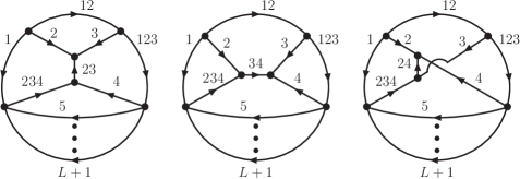
Figure 1: Diagrams of the $\rm N^{4}MLT$ family. The diagram on the l.h.s. corresponds to the $t$ channel, the diagram on the center is the $s$ channel and the diagram on the r.h.s. corresponds to the $u$ channel. An arbitrary number of external particles (not shown) are attached.

This arrangement allows to restrict the overall assessment to the N⁴MLT family that consists of three main topologies. These topologies were checked with QGRAF Nogueira:1991ex and are shown in Fig. 1. Two of them are planar and one is nonplanar. Nicely, we observe the similarity of these topologies with the insertion of a four-point subamplitude with trivalent vertices into a larger topology. Therefore, in order to achieve a unified description the three N⁴MLT topologies are interpreted as the $t$-, $s$- and $u$-kinematic channels, respectively, of a universal topology.

The three topologies contain $L+4$ common sets of propagators, and one extra set which is different for each of them. Each of the first $L$ sets depends on one characteristic loop momentum $\ell_{s}$ and the momenta of their propagators have the form $q_{i_{s}}=\ell_{s}+k_{i_{s}}$. The remaining four common sets are established as linear combinations of the loop momenta, explicitly

$$q_{i_{(L+1)}} =-\sum_{s=1}^{L}\ell_{s}+k_{i_{(L+1)}}\,,\quad q_{i_{12}}=-\ell_{1}-\ell_{2}+k_{i_{12}}\,,$$

$$q_{i_{123}} =-\sum_{s=1}^{3}\ell_{s}+k_{i_{123}}\,,\quad q_{i_{234}}=-\sum_{s=2}^{4}\ell_{s}+k_{i_{234}}\,,$$ (8)

with $k_{i_{s}},k_{i_{(L+1)}},k_{i_{12}},k_{i_{123}}$ and $k_{i_{234}}$ linear combinations of external momenta. The extra sets are the distinctive key to each of the channels in the universal topology. We identify the momenta of their propagators as different linear combinations of $\ell_{2}$, $\ell_{3}$ and $\ell_{4}$, writing them as

$$q_{i_{rs}} =-\ell_{r}-\ell_{s}+k_{i_{rs}}\,,\quad r,s\in\{2,3,4\}\,.$$ (9)

To assemble the three N⁴MLT channels into a single topology, we define the current $J$ that includes the three different type of sets,

$$J\equiv 23\cup 34\cup 24~{}.$$ (10)

Notice that due to momentum conservation, the three subsets cannot contribute to the same individual Feynman diagram but they all contribute at amplitude level. Relying on the development of this framework, the Feynman representation of the N⁴MLT universal topology can be expressed as

$$\mathcal{A}_{\rm N^{4}MLT}^{(L)}(1,\ldots,L+1,12,123,234,J)=\int_{\ell_{1},\dots,\ell_{L}}\mathcal{A}_{F}^{(L)}(1,\dots,L+1,12,123,234,J)~{}.$$ (11)

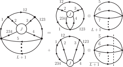
Figure 2: Diagrammatic representation for the factorized opening of the multiloop N⁴MLT universal topology. Only the on-shell cut of the last MLT-like subtopology with reversed momentum flow is shown.

The dual opening of this topology fulfills a factorization identity in terms of convoluted subtopologies, similar to those presented in Ref. Verdugo:2020kzh for NMLT and N²MLT, i.e.

$${\cal A}^{(L)}_{\rm N^{4}MLT} (1,\ldots,L+1,12,123,234,J)$$

$$={\cal A}^{(4)}_{\rm N^{4}MLT}(1,2,3,4,12,123,234,J)\otimes{\cal A}_{\rm MLT}^{(L-4)}(5,\dots,L+1)$$

$$+{\cal A}^{(3)}_{\rm N^{2}MLT}(1\cup 234,2,3,4\cup 123,12,J)\otimes{\cal A}_{\rm MLT}^{(L-3)}(\overline{5},\dots,\overline{L+1})~{}.$$ (12)

The convolution symbol indicates that each of the convoluted components is open independently, whereas the on-shell conditions from all components act together on the numerator and the propagators that remain off-shell. An essential constraint to be meet by the selected on-shell propagators concerns the non-feasibility of generating disjoint trees in the dual opening. In order to make the notation more readable, ${\cal A}^{(L)}_{{\rm N}^{k-1}{\rm MLT}}$ will refer in the following to the integrand of the corresponding topology in the LTD representation; integration over the $L$ loop momenta will be implicitly understood.

The factorization identity in Eq. (3) is the main result of this paper, and it is the universal identity that opens any multiloop N⁴MLT topology to nondisjoint trees. It also enables to infer the causal structure of the complete topology by exploring the causal behaviour of its subtopologies. Let us emphasize that this identity is valid regardless of the internal configuration, i.e. numerators, multiple-power propagators and number of external particles, because the residue operator is implicitly considered. In addition, since it properly accounts for all N^k-1MLT configurations with $k\leq 4$, it is the only master expression required to open to nondisjoint trees any scattering amplitude of up to four loops. Beyond four loops, new topologies arise which, for consistency, will include this universal topology as a particular case.

A graphical interpretation of the factorization identity is shown in Fig. 2. The term $\mathcal{A}^{(4)}_{\rm N^{4}MLT}$ on the r.h.s. of Eq. (3) considers all possible configurations with four on-shell propagators in the sets $\{1,2,3,4,12,123,234,J\}$, while ${\cal A}^{(3)}_{\rm N^{2}MLT}$ in the second term assumes three on-shell conditions under the constraints explained below. The term ${\cal A}_{\rm MLT}^{(L-4)}(5,\dots,L+1)$ is open according to the MLT opening presented in Ref. Verdugo:2020kzh ; Aguilera-Verdugo:2020nrp , and in ${\cal A}_{\rm MLT}^{(L-3)}(\overline{5},\dots,\overline{L+1})$ all the momentum flows are reversed and all the sets contain one on-shell propagator. The reversion is imposed by the fact that, in the absence of propagators in the sets $\{12,123,234,J\}$, the master opening in Eq. (3) should coincide with the MLT opening.

The factorization identity in Eq. (3) has been first tested by explicitly computing the nested residues on the l.h.s. for specific internal configurations, and then confronting the result with the unfolding (according to the known expressions of the corresponding subtopologies) of the Ansatz on the r.h.s., which is motivated by the graphical interpretation. In order to prove that Eq. (3) holds for an arbitrary number of loops, we decomposed the N⁴MLT into two parts: the upper part in the l.h.s. of Fig. 2 containing the current $J$, which encodes the novel topological complexity arising in this class of diagrams, and the lower one, which represents a known MLT-like component. The LTD representation of the topological complexity part is computed at four loops for each configuration described by the current $J$, or equivalently, by considering the MLT-like sector as a single internal line. Then, we just need to rely on the MLT formula presented in Eq. (7) to complete the calculation and obtain the all-order expression.

We have to mention certain arbitrariness in the expression (3) due to the freedom in the order of the nested application of the Cauchy residue theorem. Although there are at least $L!$ possibilities, all potential LTD representations are, however, equivalent and lead to the same causal expression in terms of dual propagators Aguilera-Verdugo:2020kzc (see Sec.4).

The four-loop subtopology in Eq. (3) is opened as well through a factorization identity which is written in terms of known subtopologies,

$$\mathcal{A}_{\rm N^{4}MLT}^{(4)}(1,2,3,4,12,123,234,J) =\mathcal{A}_{\rm{N^{2}MLT}}^{(4)}(1,2,3,4,12,123,234)\otimes\mathcal{A}^{(0)}(J)$$

$$+\sum_{{\bf s}\in J}\mathcal{A}_{D}^{(4)}(1,2,3,4,12,123,234,{\bf s})\,,$$ (13)

The diagrammatic representation of Eq. (3) is depicted in Fig. 3. The first term on the r.h.s. of Eq. (3) consists of a four-loop $\rm{N^{2}MLT}$ subtopology and describes dual trees where all the propagators with momenta in $J$ remain off shell, corresponding to the first diagram on the r.h.s. of Fig. 3. The second term on the r.h.s. of Eq. (3) collects contributions where propagators in either $23$, $34$ or $24$ are set on shell. These dual trees are therefore specific to the $t$, $s$ and $u$ channels, whose explicit expressions are presented below. We use the bold symbol ${\bf s}$ to clearly indicate that these contributions are those containing on-shell propagators in the $J$-sets.

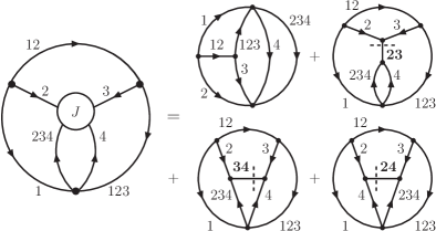
Figure 3: Diagrammatic representation of the four-loop subtopology ${\cal A}^{(4)}_{\rm N^{4}MLT}(1,2,3,4,12,123,234,J)$. The dashed lines and bold labels indicate that propagators in the $J$-sets are set on shell in either of the two momentum flows.

The three-loop subtopology on the r.h.s. of Eq. (3) is also opened in terms of known subtopologies through the factorized identity

$${\cal A}^{(3)}_{\rm N^{2}MLT}(1\cup 234,2,3,4\cup 123,12,J) =\mathcal{A}_{\rm{NMLT}}^{(3)}(1\cup 234,2,3,4\cup 123,12)\otimes\mathcal{A}^{(0)}(J)$$

$$+\sum_{{\bf s}\in J}\mathcal{A}_{D}^{(3)}(1,2,3,4,12,123,234,{\bf s})\,,$$ (14)

which has a similar structure to Eq. (3). The diagrammatic representation of Eq. (3) is depicted in Fig. 4. Similarly to Fig. 3, the first diagram on the r.h.s. of Fig. 4, which represents the first term on the r.h.s. of Eq. (3), is a three-loop NMLT subtopology and all the propagators in $J$ are off shell, while the remaining three diagrams are specific to each of the three channels. The NMLT subtopology is made up of 7 subsets of momenta grouped into 5 sets as follows $\left\{1\cup 234,2,3,4\cup 123,12\right\}$. This construction prevents, for example, that propagators in the sets $1$ and $234$ are set on shell simultaneously.

Turning back into Eqs. (3) and (3) in a more detailed way, the first terms on the r.h.s. of both equations are composed of dual contributions where all the propagators in $J$ remain off shell. These $J$-propagators act as spectators in relation to the opening of the accompanying subtopology, and can eventually be replaced by a contact interaction to deduce the opening rule of these contributions.

Specifically, the four-loop N²MLT subamplitude in Eq. (3) is represented by

$$\mathcal{A}_{\rm{N^{2}MLT}}^{(4)}(1,2,3,4,12, 123,234)=\mathcal{A}_{\rm{NMLT}}^{(3)}(1,2,3,12,123,234)\otimes\mathcal{A}_{\rm{MLT}}^{(1)}(4,234)$$

$$+\left[\mathcal{A}_{\rm{MLT}}^{(2)}(1,2,12)+\mathcal{A}^{(2)}_{\rm MLT}(1,\overline{3})\right]\otimes\mathcal{A}^{(2)}_{\rm MLT}(\overline{4},\overline{234})$$

$$+\left[\mathcal{A}_{\rm{MLT}}^{(2)}(\overline{123},\overline{3},12)+\mathcal{A}^{(2)}_{\rm MLT}(2,\overline{123})\right]\otimes\mathcal{A}^{(2)}_{\rm MLT}(4,234)\,.$$ (15)

All the MLT subamplitudes that involve a number of loops equal to the number of sets require to set on shell propagators in all the sets. The rest of NMLT and MLT subtopologies are open according to known expressions Verdugo:2020kzh . To simplify the presentation, we have omitted in Eq. (3) the explicit reference to the sets with all their propagators off shell; for instance, the element $\mathcal{A}^{(2)}_{\rm MLT}(1,\overline{3})\otimes\mathcal{A}^{(2)}_{\rm MLT}(\overline{4},\overline{234})$ must be interpreted as

$$\mathcal{A}^{(2)}_{\rm MLT} (1,\overline{3})\otimes\mathcal{A}^{(2)}_{\rm MLT}(\overline{4},\overline{234})=\mathcal{A}_{D}^{(4)}(1,\overline{3},\overline{4},\overline{234};2,12,123)\,.$$ (16)

This notation will be used in the following; the omitted sets are understood to be off shell.

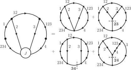
Figure 4: Diagrammatic representation of the three-loop subtopology ${\cal A}^{(3)}_{\rm N^{2}MLT}(1\cup 234,2,3,4\cup 123,12,J)$. The dashed lines and bold labels indicate that propagators in the $J$-sets are set on shell in either of the two momentum flows.

The three-loop ${\rm NMLT}$ subtopology in Eq. (3) is generated from 7 subsets clustered as $\{1\cup 234,2,3,4\cup 123,12\}$ and its LTD representation is

$$\mathcal{A}_{\rm{NMLT}}^{(3)}(1\cup 234,2,3,4\cup 123,12) =\mathcal{A}_{\rm{MLT}}^{(2)}(1\cup 234,2,12)\otimes\mathcal{A}_{\rm{MLT}}^{(1)}(3,4\cup 123)$$

$$+\mathcal{A}_{\rm{MLT}}^{(1)}(1\cup 234,2)\otimes\mathcal{A}^{(2)}_{\rm MLT}(\overline{3},\overline{4}\cup\overline{123}),$$ (17)

where the first term is a convolution of two MLT subtopologies, and in the second term all the propagators in the set $12$ are off shell.

3.1 The t channel

The second terms in Eqs. (3) and (3) distinguish the dual configurations arising for each of the three channels when propagators with momenta in $J$ are set on shell. We begin analyzing the dual terms related exclusively to the topology known as $t$ channel from Fig. 1 (left). There is one four-loop subtopology

$$\mathcal{A}_{D}^{(4)}(1,2,3,4,12, 123,234,{\bf 23})=\left[\left(\mathcal{A}_{\rm{MLT}}^{(2)}(\overline{123},\overline{3},12)+\mathcal{A}^{(2)}_{\rm MLT}(2,\overline{123})\right)\otimes\mathcal{A}^{(1)}_{D}(23)\right.$$

$$+\left.\left(\mathcal{A}_{\rm{MLT}}^{(2)}(1,2,12)+\mathcal{A}^{(2)}_{\rm MLT}(1,\overline{3})\right)\otimes\mathcal{A}^{(1)}_{D}(\overline{23})\right]\otimes\mathcal{A}^{(1)}_{\rm MLT}(4,234)~{},$$ (18)

and one three-loop subtopology

$$\mathcal{A}_{D}^{(3)}(1,2,3,4,12, 123,234,{\bf 23})=\left[\mathcal{A}_{\rm{MLT}}^{(2)}(\overline{4}\cup\overline{123},\overline{3},12)+\mathcal{A}^{(2)}_{\rm MLT}(2,\overline{4}\cup\overline{123})\right]\otimes\mathcal{A}^{(1)}_{D}(23)$$

$$+\left[\mathcal{A}_{\rm{MLT}}^{(2)}(1\cup 234,2,12)+\mathcal{A}^{(2)}_{\rm MLT}(1\cup 234,\overline{3})\right]\otimes\mathcal{A}^{(1)}_{D}(\overline{23})~{},$$ (19)

that contribute to Eqs. (3) and (3), respectively. Notice that both expressions, Eq. (18) and Eq. (19), contain on-shell propagators in the set $23$, and we have contributions with the original momentum flow, $23$, and the reversed one $\overline{23}$.

3.2 The s channel

In order to obtain the terms that characterize the $s$ channel shown in Fig. 1 (center), we set on shell a propagator in the set $34$. The four-loop subtopology is given by

$$\mathcal{A}_{D}^{(4)}(1,2,3,4,12,123,234,{\bf 34})$$

$$=\left[\mathcal{A}_{\rm{NMLT}}^{(3)}(1,2,3,12,123)+\mathcal{A}^{(3)}_{\rm MLT}(\overline{3},\overline{123},234)\right.$$

$$+\mathcal{A}_{\rm{MLT}}^{(2)}(1,2,12)\otimes\mathcal{A}^{(1)}_{D}(\overline{4})+\left.\mathcal{A}_{\rm{MLT}}^{(1)}(3\cup\overline{4},123)\otimes\mathcal{A}^{(2)}_{\rm MLT}(\overline{12},234)\right]\otimes\mathcal{A}^{(1)}_{D}(\overline{34})$$

$$+\left[\mathcal{A}_{\rm{MLT}}^{(1)}(3\cup\overline{4},123)\otimes\mathcal{A}^{(2)}_{\rm MLT}(1,\overline{234})\right.+\left.\mathcal{A}_{\rm{MLT}}^{(1)}(1,2\cup\overline{234})\otimes\mathcal{A}^{(2)}_{\rm MLT}(4,\overline{123})\right]\otimes\mathcal{A}^{(1)}_{D}(34)\,.$$ (20)

This expression is more involved than the corresponding one in the $t$ channel, because the loop momentum $\ell_{4}$ is now present in three sets, while in the $t$ channel $\ell_{4}$ is found in two sets only.

By contrast, for the three-loop subamplitude we observe a very symmetric structure which allows to avoid any momentum flow reversion. In this case, we end up with an expression that only depends on the original momentum flow of the set $34$,

$$\mathcal{A}_{D}^{(3)}(1,2,3,4,12,123,234,{\bf 34})=\mathcal{A}_{\rm{MLT}}^{(1)}(1\cup 234,2)\otimes\mathcal{A}_{\rm{MLT}}^{(1)}(3,4\cup 123)\otimes\mathcal{A}^{(1)}_{D}(34)\,.$$ (21)

Given the structure of this subtopology, it is manifest that propagators in 12 and 34 cannot become on shell simultaneously without generating a disjoint tree, as expected from Fig. 4.

3.3 The u channel

Moving on to the last terms associated to the nonplanar topology known as $u$ channel (Fig. 1 (right)), the LTD representation of the four-loop subamplitude with on-shell propagators in the set $24$ reads

$$\mathcal{A}_{D}^{(4)} (1,2,3,4,12,123,234,{\bf 24})$$

$$=\left[\mathcal{A}_{\rm{NMLT}}^{(3)}(1,2,3,12,123)\right.+\mathcal{A}_{\rm{MLT}}^{(1)}(1,2\cup\overline{4})\otimes\mathcal{A}^{(2)}_{\rm MLT}(\overline{123},234)$$

$$+\left.\mathcal{A}_{\rm{MLT}}^{(1)}(3\cup\overline{234},123)\otimes\mathcal{A}^{(2)}_{\rm MLT}(1,\overline{4})\right]\otimes\mathcal{A}^{(1)}_{D}(\overline{24})$$

$$+\left[\mathcal{A}_{\rm{MLT}}^{(2)}(1,2,12)\otimes\mathcal{A}^{(1)}_{\rm MLT}(\overline{234})+\mathcal{A}^{(3)}_{\rm MLT}(4,\overline{3},\overline{123})\right.$$

$$+\left.\mathcal{A}_{\rm{MLT}}^{(1)}(3\cup\overline{234},123)\otimes\mathcal{A}^{(2)}_{\rm MLT}(4,\overline{12})\right]\otimes\mathcal{A}^{(1)}_{D}(24)\,.$$ (22)

This subtopology is also not as compact as the expression for the $t$ channel because $\ell_{4}$ is also present in three different sets. For the three-loop subamplitude, we find,

$$\mathcal{A}_{D}^{(3)}(1,2,3,4,12,123,234,{\bf 24}) =\left[\mathcal{A}^{(2)}_{\rm MLT}(1\cup 234,\overline{4})+\mathcal{A}^{(2)}_{\rm MLT}(234,\overline{123})\right]\otimes\mathcal{A}^{(1)}_{D}(\overline{24})$$

$$+\left[\mathcal{A}_{\rm{MLT}}^{(2)}(1\cup 234\cup\overline{3},2,12)+\mathcal{A}^{(2)}_{\rm MLT}(\overline{3},\overline{4}\cup\overline{123})\right.$$

$$+\left.\mathcal{A}^{(2)}_{\rm MLT}(4\cup 123,\overline{12})+\mathcal{A}^{(2)}_{\rm MLT}(\overline{1},123)\right]\otimes\mathcal{A}^{(1)}_{D}(24)~{}.$$ (23)

All these results are consistent with the absence of disjoint trees. We would like to comment on the fact that repeated propagators from selfenergy insertions are treated as single propagators raised to specific powers and are not considered to generate disjoint trees when the repeated propagator is set on shell.

Notice that the number of trees in the LTD forest can also be computed through the combinatorial exercise of selecting, from the full list of sets, all possible subsets of $L$ elements that cannot generate disjoint trees. For the individual $t$, $s$ and $u$ channels the number of terms calculated in this way are $5(8L-17)$, $15(3L-7)$ and $9(5L-11)$, respectively, and $82L-187$ for the N⁴MLT universal topology, in agreement with the number of dual contributions generated by Eq. (3). The momentum flows of the on-shell propagators, however, can only be determined through the nested residues.

4 Causal representations

The LTD representation generates in general two kind of singularities, causal thresholds that can be interpreted in terms of causality, and noncausal thresholds that are unphysical and cancel among different dual terms Buchta:2014dfa ; Aguilera-Verdugo:2019kbz . In Ref. Verdugo:2020kzh , we conjectured that, in fact, the LTD representation can be rearranged in such a way that noncausal singularities are manifestly absent in the analytic expression. In this section, we confirm the causal conjecture for the N⁴MLT family and present explicit causal representations of selected configurations that can be described through very compact analytic expressions.

We consider, in the first place, the multi-loop N³MLT configuration with one internal propagator in each loop set and five external momenta

$${\cal A}_{{\rm N}^{3}{\rm MLT}}^{(L)}(1,\ldots,L+4)=\int_{\ell_{1},\cdots,\ell_{L}}\mathcal{N}(\{\ell_{s}\}_{L},\{p_{j}\}_{N})\,G_{F}(1,\ldots,L+1,12,123,234)~{},$$ (24)

where the internal momenta are defined in Eq. (8). Its LTD representation is obtained through the universal N⁴MLT expression in Eq. (3) by considering $J$ as an empty set, or equivalently, by substituting $J$ by a contact interaction. After computing the nested residues and adding them all together, the dual representation reads

$${\cal A}_{{\rm N}^{3}{\rm MLT}}^{(L)}(1,\ldots,L+4)=\int_{\vec{\ell}_{1},\cdots,\vec{\ell}_{L}}\frac{{\cal N}_{{\rm N}^{3}{\rm MLT}}(\{q_{s,0}^{(+)},k_{j,0}\})}{x_{L+4}\left(\prod_{i=1}^{13}\lambda_{i}^{+}\lambda_{i}^{-}\right)}~{},$$ (25)

where the integrand is a function of the on-shell energies, $q_{s,0}^{(+)}=\sqrt{\mathbf{q}_{s}^{2}+m_{s}^{2}-\imath 0}$, with $s\in\{1,\ldots,L+4\}$, and the energy components of the linear combinations of external momenta, $k_{j,0}$. This is an integral in the loop three-momenta with integration measure

$$\int_{\vec{\ell}_{s}}=-\mu^{4-d}\int\frac{d^{d-1}\ell_{s}}{(2\pi)^{d-1}}~{}.$$ (26)

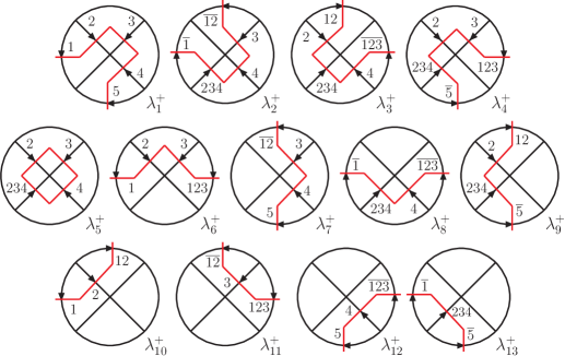
Figure 5: Causal configurations of the ${\rm N^{3}MLT}$ topology. The $\lambda_{i}^{-}$ configurations are obtained by reversing the momentum flows of the corresponding $\lambda_{i}^{+}$ configurations shown here. The set number $5$ accounts for all the propagators in the sets $5$ to $L+1$.

The integrand in Eq. (25) is written in terms of

$$x_{L+4}=\prod_{s=1}^{L+4}2q_{s,0}^{(+)}~{},$$ (27)

and the thirteen causal denominators

$$\lambda_{1}^{\pm}=q_{(1,\ldots,L+1),0}^{(+)}\pm k_{L+1,0}~{}, \lambda_{2}^{\pm}=q_{(1,12,3,4,234),0}^{(+)}\pm(k_{234}-k_{12})_{0}~{},$$

$$\lambda_{3}^{\pm}=q_{(2,4,12,123,234),0}^{(+)}\pm(k_{12}+k_{234}-k_{123})_{0}~{}, \lambda_{4}^{\pm}=q_{(2,3,123,234,5,\ldots,L+1),0}^{(+)}\pm(k_{123}+k_{234}-k_{L+1})_{0}~{},$$

$$\lambda_{5}^{\pm}=q_{(2,3,4,234),0}^{(+)}\pm k_{234,0}~{},$$

$$\lambda_{6}^{\pm}=q_{(1,2,3,123),0}^{(+)}\pm k_{123,0}~{}, \lambda_{7}^{\pm}=q_{(12,3,4,\ldots,L+1),0}^{(+)}\pm(k_{L+1}-k_{12})_{0}~{},$$

$$\lambda_{8}^{\pm}=q_{(1,4,123,234),0}^{(+)}\pm(k_{234}-k_{123})_{0}~{}, \lambda_{9}^{\pm}=q_{(2,12,234,5,\ldots,L+1),0}^{(+)}\pm(k_{12}+k_{234}-k_{L+1})_{0}~{},$$

$$\lambda_{10}^{\pm}=q_{(1,2,12),0}^{(+)}\pm k_{12,0}~{}, \lambda_{11}^{\pm}=q_{(12,3,123),0}^{(+)}\pm(k_{123}-k_{12})_{0}~{},$$

$$\lambda_{12}^{\pm}=q_{(123,4,\ldots,L+1),0}^{(+)}\pm(k_{L+1}-k_{123})_{0}~{}, \lambda_{13}^{\pm}=q_{(1,234,5,\ldots,L+1),0}^{(+)}\pm(k_{234}-k_{L+1})_{0}~{},$$ (28)

where we have defined $q_{(\alpha),0}^{(+)}=\sum_{i\in\alpha}q_{i,0}^{(+)}$. As explained in Refs. Verdugo:2020kzh ; Aguilera-Verdugo:2020kzc , these denominators are causal because they are constructed from sums of on-shell energies exclusively, and they represent potential singular configurations in which the momentum flows of the internal propagators are aligned in the same direction. The causal denominators appear in pairs because there are two opposite directions to consider for each aligned configuration. A graphical representation of these causal configurations is shown in Fig. 5. All other linear combinations of on-shell energies do not have a physical interpretation in terms of causality, and are cancelled analytically in the sum over nested residues. As a result, the straightforward application of LTD leads directly to an expression, Eq. (25), which is manifestly causal. In addition, the causal expression is independent of the initial flow assigments of the internal momenta, and of the order of the nested application of the Cauchy residue theorem.

However, the numerator of the integrand, ${\cal N}_{{\rm N}^{3}{\rm MLT}}(\{q_{s,0}^{(+)},k_{j,0}\})$, is a lengthy polynomial in the on-shell and external energies. For example, it is a polynomial of degree nine for the scalar integral. A more suitable causal expression can be obtained by reinterpreting Eq. (25) in terms of a number of entangled thresholds equal to the difference between the number of propagators and the number of loops by, e.g., analytical reconstruction from numerical evaluation over finite fields vonManteuffel:2014ixa ; Peraro:2016wsq ; Peraro:2019svx as defined in Ref. Aguilera-Verdugo:2020kzc . The N³MLT expression in Eq. (25) is analytically reconstructed by matching all combinations of four thresholds that are causally compatible to each other

$${\cal A}_{{\rm N}^{3}{\rm MLT}}^{(L)}(1,\ldots,L+4)=\int_{\vec{\ell}_{1},\cdots,\vec{\ell}_{L}}\frac{1}{x_{L+4}}\sum_{\sigma}\frac{{\cal N}_{\sigma(i_{1},\ldots,i_{4})}(\{q_{s,0}^{(+)},k_{j,0}\})}{\lambda_{\sigma(i_{1})}\lambda_{\sigma(i_{2})}\lambda_{\sigma(i_{3})}\lambda_{\sigma(i_{4})}}~{},$$ (29)

where $\lambda_{\sigma(i)}\in\{\lambda_{i}^{\pm}\}_{i=1,\ldots,13}$, and the numerators ${\cal N}_{\sigma(i_{1},\ldots,i_{4})}$ are of the same polynomial order as the original numerator in the Feynman representation, e.g., they are constants for scalar integrals. To simplify the discussion, we will present explicit results only for scalar integrals because they fully encode all the compatible causal matchings. For example, given a quadratic numerator, we can use the identity

$$\left(q_{i,0}\right)^{2}G_{F}(q_{i})=1+\left(q_{i,0}^{(+)}\right)^{2}G_{F}(q_{i})~{}.$$ (30)

The first term on the r.h.s. generates a scalar integral with one propagator less than the original integral, while the second term introduces a factor $\left(q_{i,0}^{(+)}\right)^{2}$ which is not modified by the application of the Cauchy residue theorem. Both integrals, however, are described by the same set of causal thresholds. In general, tensor reduction commutes with LTD and can be used to deal with tensor integrals.

The explicit expression that we obtain for the scalar N³MLT is very compact:

$${\cal A}_{{\rm N}^{3}{\rm MLT}}^{(L)}(1,\ldots,L+4)=\int_{\vec{\ell}_{1},\cdots,\vec{\ell}_{L}}\frac{1}{x_{L+4}}\bigg{[}{\cal F}^{(L+4)}_{(1,5,6,7,10,11,12,13)}+{\cal F}^{(L+4)}_{(2,5,7,8,11,12,13,10)}$$

$$\qquad+{\cal F}^{(L+4)}_{(3,5,8,9,12,13,10,11)}+{\cal F}^{(L+4)}_{(4,5,9,6,13,10,11,12)}+L^{+}_{(6,10,11)}L^{-}_{(8,12,13)}$$

$$\qquad+L^{-}_{(7,11,12)}L^{+}_{(9,13,10)}+L^{+}_{10}L^{-}_{11}L^{+}_{12}L^{-}_{13}+(\lambda_{i}^{+}\leftrightarrow\lambda_{i}^{-})\bigg{]}~{},$$ (31)

where

$${\cal F}^{(L+4)}_{(1,5,6,7,10,11,12,13)}=L^{+}_{1}\left(L^{+}_{5}+L^{-}_{13}\right)\left(L^{+}_{(6,10,11)}+L^{+}_{(7,11,12)}+L^{+}_{10}L^{+}_{12}\right)~{},$$

with

$$L_{i}^{\pm}=\frac{1}{\lambda_{i}^{\pm}}~{},\qquad L_{(i,j,k)}^{\pm}=L^{\pm}_{i}\left(L^{\pm}_{j}+L^{\pm}_{k}\right)~{}.$$ (33)

The function ${\cal F}^{(L+4)}$ encodes four causal configurations that are obtained by permutation of the arguments. The number of terms generated by Eq. (3) scales as $3(8L-17)$, i.e. 45 terms at four loops, while the number of terms generated by Eq. (31) equals $98$ regardless of the number of loops. The numerical performance of Eq. (31) is, in addition, a factor $2$ to $8$ faster than Eq. (3) at four loops, and even three orders of magnitude faster than Eq. (25). We have estimated the numerical performance by comparing the timings of evaluating the integrands at $1000$ random points. Similar relative timing are observed for the rest of the configurations presented in this paper.

Let us emphasize that the most significant advantage of Eq. (31) with respect to Eq. (3) stems from the core difference between them, the presence or absence of noncausal singularities. The straightforward application of the nested residue generates multiple threshold singularities, nevertheless, with a clever analytical rearrangement, the absence of noncausal singularities is achieved and leads to a causal representation which is more efficient and stable numerically in all the integration domain. To illustrate the impact of noncausal singularities, we present in Fig. 6 the integrand of the dual representation of the N³MLT vacuum diagram ($k_{j,0}=0$) as a function of the two on-shell energies $q_{12,0}^{(+)}$ and $q_{123,0}^{(+)}$ where the remaining on-shell energies are set at fixed values, $q_{i,0}^{(+)}=1$ for $i=1,\dots,5$ and $q_{234,0}^{(+)}=2$. The white lines represent the location of the noncausal thresholds which arise due to the denominators $1/(q_{12,0}^{(+)}-q_{i,0}^{(+)})$, $1/(q_{123,0}^{(+)}-q_{i,0}^{(+)})$ and $1/(q_{12,0}^{(+)}-q_{123,0}^{(+)}\pm q_{i,0}^{(+)})$. Additionally, to clarify the meaning of the noncausal thresholds in Fig. 6 in more detail, we study one of the singularities by fixing $q_{123,0}^{(+)}$ and scanning over $q_{12,0}^{(+)}$. The results of noncausal and causal evaluations of the N³MLT configurations are displayed in Fig. 7 in the left and right plots, respectively. Similar findings were reported in Ref. Aguilera-Verdugo:2020kzc , where explicit causal representations of up to N²MLT complexity were presented.

In return, the LTD representation in Eq. (3) is universal and valid regardless of the internal configuration, while the causal representation is specific to the details of the configuration under consideration, e.g., the number of propagators in each loop set. The number of terms for a given N^k-1MLT topology in Eq. (3) scales with the number of loops and linearly with the number of propagators per loop set, but the sum over residues, equivalently over internal propagators, is implicitly accounted in this expression. By contrast, the number of terms for a given N^k-1MLT topology is independent of the number of loops in the causal representation but requires to specify additional causal thresholds and additional causal entanglements when more internal propagators are considered. In this respect, external momenta attached to interaction vertices that connect different loop sets do not alter the number of internal propagators and therefore the complexity of the causal representation. We will exploit this feature in the following to simplify the discussion of the causal representation of the N⁴MLT topology. The full causal expressions with external momenta can be deduced from the causal representation of the vacuum configuration by matching the momentum flows of the entangled thresholds.

Figure 6: Integrand-level behaviour of the noncausal LTD representation of a four-loop N³MLT diagram. White lines indicate the position of noncausal thresholds.

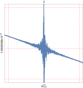
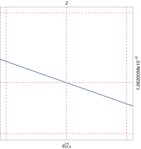
Figure 7: Numerical instabilities of the four-loop N³MLT integrand which arise due to noncausal singularities (left), which are absent in the causal representations (right).

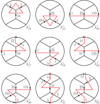
Figure 8: Extra causal configurations of the $t$-channel of the ${\rm N^{4}MLT}$ topology.

Let us then consider the $t$-channel of the N⁴MLT universal topology

$${\cal A}_{{\rm N}^{4}{\rm MLT}}^{(L)}(1,\ldots,L+4,23)=\int_{\ell_{1},\cdots,\ell_{L}}\mathcal{N}(\{\ell_{s}\}_{L},\{p_{j}\}_{N})\,G_{F}(1,\ldots,L+4,23)~{},$$ (34)

again with only one propagator per set, and six external particles. Its LTD representation is causal after all the nested residues are summed up together, i.e.

$${\cal A}_{{\rm N}^{4}{\rm MLT}}^{(L)}(1,\ldots,L+4,23)=\int_{\vec{\ell}_{1},\cdots,\vec{\ell}_{L}}\frac{{\cal N}_{{\rm N}^{4}{\rm MLT}}(\{q_{s,0}^{(+)},k_{j,0}\})}{x_{t,L+5}\left(\prod_{i=1}^{22}\lambda_{i}^{+}\lambda_{i}^{-}\right)}~{},$$ (35)

where $x_{t,L+5}=2q_{23,0}^{(+)}\,x_{L+4}$. The LTD representation in Eq. (35) depends on the causal denominators already defined for the N³MLT configuration in Eq. (28) in addition to nine extra causal denominators that depend on $q_{23,0}^{(+)}$ (the corresponding configurations are shown in Fig. 8):

$$\lambda_{14}^{\pm}=q_{(2,3,23),0}^{(+)}\pm k_{23,0}~{}, \lambda_{15}^{\pm}=q_{(4,234,23),0}^{(+)}\pm(k_{234}-k_{23})_{0}~{},$$

$$\lambda_{16}^{\pm}=q_{(1,123,23),0}^{(+)}\pm(k_{123}-k_{23})_{0}~{}, \lambda_{17}^{\pm}=q_{(1,3,12,23),0}^{(+)}\pm(k_{23}-k_{12})_{0}~{},$$

$$\lambda_{18}^{\pm}=q_{(1,4,\ldots,L+1,23),0}^{(+)}\pm(k_{L+1}-k_{23})_{0}~{},$$

$$\lambda_{19}^{\pm}=q_{(2,12,123,23),0}^{(+)}\pm(k_{12}+k_{23}-k_{123})_{0}~{},$$

$$\lambda_{20}^{\pm}=q_{(123,234,5,\ldots,L+1,23),0}^{(+)}\pm(k_{123}+k_{234}-k_{L+1}-k_{23})_{0}~{},$$

$$\lambda_{21}^{\pm}=q_{(2,4,\ldots,L+1,12,23),0}^{(+)}\pm(k_{12}+k_{23}-k_{L+1})_{0}~{},$$

$$\lambda_{22}^{\pm}=q_{(3,5,\ldots,L+1,12,234,23),0}^{(+)}\pm(k_{234}+k_{12}-k_{23}-k_{L+1})_{0}~{}.$$ (36)

The numerator in Eq. (35) is now a polynomial of degree seventeen for the scalar integral. We should consider then all the entangled configurations with five causal thresholds. For the sake of simplicity, we will restrict the analysis to the vacuum configuration, which implies $\lambda_{i}^{+}=\lambda_{i}^{-}$ and is sufficient to have a clear overview of the causal structure, as explained before. Applying the reconstruction algorithm defined in Ref. Aguilera-Verdugo:2020kzc , we obtain again a very compact result, and an overall structure similar to Eq. (31),

$${\cal A}_{{\rm N}^{4}{\rm MLT}}^{(L)}(1,\ldots,L+4,23)=-\int_{\vec{\ell}_{1},\cdots,\vec{\ell}_{L}}\frac{2}{x_{t,L+5}}\bigg{[}{\cal F}^{(L+5)}_{(1,5,6,7,10,11,12,13,14,15,18)}$$

$$\quad+{\cal F}^{(L+5)}_{(2,5,7,8,11,12,13,10,15,14,17)}+{\cal F}^{(L+5)}_{(3,5,8,9,12,13,10,11,15,14,19)}+{\cal F}^{(L+5)}_{(4,5,9,6,13,10,11,12,14,15,20)}$$

$$\quad+{\cal F}^{(L+5)}_{(21,18,19,7,14,11,12,9,13,15,10)}+{\cal F}^{(L+5)}_{(22,17,20,7,15,12,11,9,10,14,13)}$$

$$\quad+{\cal G}^{(L+5)}_{(10,14,6,13,11,12,15,8)}+{\cal G}^{(L+5)}_{(10,11,12,13,14,15,17,18)}+{\cal G}^{(L+5)}_{(12,13,10,11,15,14,20,19)}$$

$$\quad+\left(L_{(6,10,11)}+L_{(17,10,14)}+L_{(19,11,14)}\right)\left(L_{(8,12,13)}+L_{(18,13,15)}+L_{(20,12,15)}\right)L_{16}\bigg{]}~{},$$

(37)

that is written in terms of permutations of the arguments of the two functions

$${\cal F}^{(L+5)}_{(1,\ldots,11)} = L_{1}\left(L_{(2,9,10)}+L_{(8,9,11)}+L_{10}\,L_{11}\right)\left(L_{(3,5,6)}+L_{(4,6,7)}+L_{5}\,L_{7}\right)~{},$$ (38)

and

$${\cal G}^{(L+5)}_{(1,\ldots,8)}=\left(L_{1}+L_{5}\right)\,L_{(3,4,6)}\,L_{(7,2,8)}~{}.$$ (39)

Notice that, for example

$$\left.{\cal F}^{(L+5)}_{(1,5,6,7,10,11,12,13,14,15,18)}\right|_{L_{14}\rightarrow 1,(L_{15},L_{18})\rightarrow 0}={\cal F}^{(L+4)}_{(1,5,6,7,10,11,12,13)}~{},$$ (40)

thus ensuring the consistency of Eq. (37) with Eq. (31).

The $s$-channel is obtained just by a clockwise rotation of the $t$-channel and therefore by a permutation of the arguments of the causal denominators that are channel specific

$$\lambda_{i}^{\pm}(1,2,3,4,5\cdots(L+1),12,123,234,34)$$

$$\qquad=\lambda_{i}^{\pm}(\overline{5\cdots(L+1)},234,2,3,123,\overline{1},12,4,23)~{},\qquad i\in[14,22]~{}.$$ (41)

This means that in Eq. (36) it is enough to make, for example, replacements similar to

$$\lambda_{14}^{\pm}\rightarrow q_{(3,4,34),0}^{(+)}\pm k_{34,0}~{}.$$

$$\lambda_{18}^{\pm}\rightarrow q_{(1,12,234,34),0}^{(+)}\pm(k_{234}-k_{12}-k_{34})_{0}~{},$$ (42)

to obtain the corresponding causal representation.

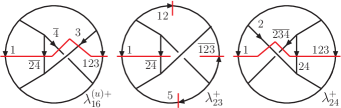
Figure 9: Extra causal configurations of the $u$-channel of the ${\rm N^{4}MLT}$ topology due to nonplanarity.

For the $u$-channel, the causal denominators are obtained from the $t$-channel through the substitution $23\rightarrow 24$ and by the exchange $3\leftrightarrow 4$ or $2\leftrightarrow 234$ ($123$ remains invariant):

$$\lambda_{i}^{\pm}(1,\ldots,L+1,12,123,234,24) = \lambda_{i}^{\pm}(3\leftrightarrow 4,23\rightarrow 24)~{},\qquad i\in[14,15,17,18,22]~{},$$

$$\lambda_{i}^{\pm}(1,\ldots,L+1,12,123,234,24) = \lambda_{i}^{\pm}(2\leftrightarrow 234,23\rightarrow 24)~{},\qquad i\in[19,20,21]~{}.$$ (43)

There are, however, three new configurations that arise because the $u$-channel is nonplanar. These new configurations are shown in Fig. 9 and are described by the following causal denominators

$$\lambda_{16}^{(u)\pm}=q_{(1,\ldots,4,123),0}^{(+)}\pm k_{123,0}~{},$$

$$\lambda_{23}^{\pm}=q_{(1,5,\ldots,L+1,12,123,24),0}^{(+)}\pm(k_{L+1}+k_{12}-k_{123}-k_{24})_{0}~{},$$

$$\lambda_{24}^{\pm}=q_{(1,2,123,234,24),0}^{(+)}\pm(k_{123}-k_{234}+k_{24})_{0}~{}.$$ (44)

The causal representation of the $u$-channel has a very similar structure to Eq. (37)

$${\cal A}_{{\rm N}^{4}{\rm MLT}}^{(L)}(1,\ldots,L+4,24)=-\int_{\vec{\ell}_{1},\cdots,\vec{\ell}_{L}}\frac{2}{x_{u,L+5}}\bigg{[}{\cal F}^{(L+5)}_{(1,5,6,7,10,11,12,13,14,15,18)}$$

$$\quad+{\cal F}^{(L+5)}_{(2,5,7,8,11,12,13,10,15,14,17)}+{\cal F}^{(L+5)}_{(3,5,8,9,12,13,10,11,14,15,19)}+{\cal F}^{(L+5)}_{(4,5,9,6,13,10,11,12,15,14,20)}$$

$$\quad+{\cal F}^{(L+5)}_{(21,18,20,7,14,12,11,9,13,15,10)}+{\cal F}^{(L+5)}_{(22,17,19,7,15,11,12,9,10,14,13)}+{\cal F}^{(L+5)}_{(16,18,17,6,14,10,11,8,13,15,12)}$$

$$\quad+{\cal F}^{(L+5)}_{(24,20,19,6,15,11,10,8,12,14,13)}+{\cal F}^{(L+5)}_{(23,19,20,17,12,14,10,18,15,11,13)}$$

$$\quad+L_{10}\,L_{12}\,L_{15}\left(L_{11}\,L_{13}+L_{11}\,L_{14}+L_{13}\,L_{14}\right)\bigg{]}~{},$$ (45)

where $x_{u,L+5}=2q_{24,0}^{(+)}\,x_{L+4}$.

5 Conclusions

We have analized the multiloop topologies that appear for the first time at four loops and have found a general representation, the N⁴MLT universal topology, which describes their opening to nondisjoint trees through the loop-tree duality. The opening to trees admits a very structured and compact factorized interpretation in terms of convolutions of known subtopologies, that finally determine the internal causal structure of the entire amplitude. The LTD representation presented in this paper is valid in arbitrary coordinate systems and space-time dimensions.

The N⁴MLT topology is called universal because it unifies in a single expression all the necessary ingredients to open any scattering amplitude of up to four loops. Beyond four loops, this topology will be embedded in more complex topologies, so that the methodology presented here can be used as a guide to achieve a full description of higher orders.

We have verified that the LTD representation of N⁴MLT is manifestly causal, namely, that the explicit LTD analytic expression is inherently free of noncausal singularities. On the one hand, this supports the applicability and generalization of four-dimensional unsubtraction to higher orders. On the other hand, it allows a more efficient numerical evaluation of multiloop scattering amplitudes than other integrand representations due to the absence of noncausal singularities. These results extend by one perturbative order the causal analysis of Ref. Aguilera-Verdugo:2020kzc , and the interpretation of LTD in terms of entangled causal thresholds. In addition, they confirm the all-order conjectures of Ref. Verdugo:2020kzh . We expect similar conclusions at higher orders, thus leading to a noticeable improvement in the available toolkit for computing highly-precise theoretical predictions.

6 Acknowledgments

This work is supported by the Spanish Government (Agencia Estatal de Investigación) and ERDF funds from European Commission (Grant No. FPA2017-84445-P), Generalitat Valenciana (Grant No. PROMETEO/2017/053), and the COST Action CA16201 PARTICLEFACE. S. R.-U. from CONACYT and Universidad Autónoma de Sinaloa; W.J.T. from Juan de la Cierva program (FJCI-2017-32128); and R. J. H.-P. from Departament de Física Teòrica, Universitat de València, CONACyT through the Project No. A1-S-33202 (Ciencia Básica) and Sistema Nacional de Investigadores.

References

- (1) M. Mangano, LHC at 10: the physics legacy, 2003.05976.
- (2) FCC collaboration, A. Abada et al., FCC Physics Opportunities: Future Circular Collider Conceptual Design Report Volume 1, Eur. Phys. J. C 79 (2019) 474.
- (3) FCC collaboration, A. Abada et al., FCC-ee: The Lepton Collider: Future Circular Collider Conceptual Design Report Volume 2, Eur. Phys. J. ST 228 (2019) 261–623.
- (4) FCC collaboration, A. Abada et al., HE-LHC: The High-Energy Large Hadron Collider: Future Circular Collider Conceptual Design Report Volume 4, Eur. Phys. J. ST 228 (2019) 1109–1382.
- (5) FCC collaboration, A. Abada et al., FCC-hh: The Hadron Collider: Future Circular Collider Conceptual Design Report Volume 3, Eur. Phys. J. ST 228 (2019) 755–1107.
- (6) P. Bambade et al., The International Linear Collider: A Global Project, 1903.01629.
- (7) ILC collaboration, G. Aarons et al., International Linear Collider Reference Design Report Volume 2: Physics at the ILC, 0709.1893.
- (8) CLIC, CLICdp collaboration, The Compact Linear e+e- Collider (CLIC): Physics Potential, 1812.07986.
- (9) CEPC Study Group collaboration, M. Dong et al., CEPC Conceptual Design Report: Volume 2 - Physics & Detector, 1811.10545.
- (10) C. Anastasiou, C. Duhr, F. Dulat, F. Herzog and B. Mistlberger, Higgs Boson Gluon-Fusion Production in QCD at Three Loops, Phys. Rev. Lett. 114 (2015) 212001, [1503.06056].
- (11) R. Mondini, M. Schiavi and C. Williams, N3LO predictions for the decay of the Higgs boson to bottom quarks, JHEP 06 (2019) 079, [1904.08960].
- (12) B. Mistlberger, Higgs boson production at hadron colliders at N3LO in QCD, JHEP 05 (2018) 028, [1802.00833].
- (13) T. Ahmed, M. Bonvini, M. Kumar, P. Mathews, N. Rana, V. Ravindran et al., Pseudo-scalar Higgs boson production at N3 LO +N3 LL ′, Eur. Phys. J. C 76 (2016) 663, [1606.00837].
- (14) M. Bonetti, K. Melnikov and L. Tancredi, Three-loop mixed QCD-electroweak corrections to Higgs boson gluon fusion, Phys. Rev. D 97 (2018) 034004, [1711.11113].
- (15) F. A. Dreyer and A. Karlberg, Vector-Boson Fusion Higgs Production at Three Loops in QCD, Phys. Rev. Lett. 117 (2016) 072001, [1606.00840].
- (16) L. Cieri, X. Chen, T. Gehrmann, E. N. Glover and A. Huss, Higgs boson production at the LHC using the subtraction formalism at N3LO QCD, JHEP 02 (2019) 096, [1807.11501].
- (17) L. Cieri, D. de Florian, M. Der and J. Mazzitelli, Mixed QCDQED corrections to exclusive Drell Yan production using the -subtraction method, 2005.01315.
- (18) S. Catani, T. Gleisberg, F. Krauss, G. Rodrigo and J.-C. Winter, From loops to trees by-passing Feynman’s theorem, JHEP 09 (2008) 065, [0804.3170].
- (19) I. Bierenbaum, S. Catani, P. Draggiotis and G. Rodrigo, A Tree-Loop Duality Relation at Two Loops and Beyond, JHEP 10 (2010) 073, [1007.0194].
- (20) I. Bierenbaum, S. Buchta, P. Draggiotis, I. Malamos and G. Rodrigo, Tree-Loop Duality Relation beyond simple poles, JHEP 03 (2013) 025, [1211.5048].
- (21) E. Tomboulis, Causality and Unitarity via the Tree-Loop Duality Relation, JHEP 05 (2017) 148, [1701.07052].
- (22) R. Runkel, Z. Szőr, J. P. Vesga and S. Weinzierl, Causality and loop-tree duality at higher loops, Phys. Rev. Lett. 122 (2019) 111603, [1902.02135].
- (23) Z. Capatti, V. Hirschi, D. Kermanschah and B. Ruijl, Loop-Tree Duality for Multiloop Numerical Integration, Phys. Rev. Lett. 123 (2019) 151602, [1906.06138].
- (24) J. J. Aguilera-Verdugo, F. Driencourt-Mangin, R. J. Hernandez Pinto, J. Plenter, S. Ramirez-Uribe, A. E. Renteria Olivo et al., Open loop amplitudes and causality to all orders and powers from the loop-tree duality, Phys. Rev. Lett. 124 (2020) 211602, [2001.03564].
- (25) S. Buchta, G. Chachamis, P. Draggiotis, I. Malamos and G. Rodrigo, On the singular behaviour of scattering amplitudes in quantum field theory, JHEP 11 (2014) 014, [1405.7850].
- (26) J. J. Aguilera-Verdugo, F. Driencourt-Mangin, J. Plenter, S. Ramírez-Uribe, G. Rodrigo, G. F. Sborlini et al., Causality, unitarity thresholds, anomalous thresholds and infrared singularities from the loop-tree duality at higher orders, JHEP 12 (2019) 163, [1904.08389].
- (27) R. J. Hernandez-Pinto, G. F. R. Sborlini and G. Rodrigo, Towards gauge theories in four dimensions, JHEP 02 (2016) 044, [1506.04617].
- (28) G. F. R. Sborlini, F. Driencourt-Mangin, R. Hernandez-Pinto and G. Rodrigo, Four-dimensional unsubtraction from the loop-tree duality, JHEP 08 (2016) 160, [1604.06699].
- (29) G. F. R. Sborlini, F. Driencourt-Mangin and G. Rodrigo, Four-dimensional unsubtraction with massive particles, JHEP 10 (2016) 162, [1608.01584].
- (30) F. Driencourt-Mangin, Four-dimensional representation of scattering amplitudes and physical observables through the application of the Loop-Tree Duality theorem. PhD thesis, U. Valencia (main), 2019. 1907.12450.
- (31) D. E. Soper, Techniques for QCD calculations by numerical integration, Phys. Rev. D 62 (2000) 014009, [hep-ph/9910292].
- (32) R. A. Fazio, P. Mastrolia, E. Mirabella and W. J. Torres Bobadilla, On the Four-Dimensional Formulation of Dimensionally Regulated Amplitudes, Eur. Phys. J. C74 (2014) 3197, [1404.4783].
- (33) D. Z. Freedman, K. Johnson and J. I. Latorre, Differential regularization and renormalization: A New method of calculation in quantum field theory, Nucl. Phys. B 371 (1992) 353–414.
- (34) O. Battistel, A. Mota and M. Nemes, Consistency conditions for 4-D regularizations, Mod. Phys. Lett. A 13 (1998) 1597–1610.
- (35) Y.-L. Wu, Symmetry principle preserving and infinity free regularization and renormalization of quantum field theories and the mass gap, Int. J. Mod. Phys. A 18 (2003) 5363–5420, [hep-th/0209021].
- (36) R. Pittau, A four-dimensional approach to quantum field theories, JHEP 1211 (2012) 151, [1208.5457].
- (37) C. Gnendiger et al., To , or not to : recent developments and comparisons of regularization schemes, Eur. Phys. J. C77 (2017) 471, [1705.01827].
- (38) S. Pozzorini, H. Zhang and M. F. Zoller, Rational Terms of UV Origin at Two Loops, JHEP 05 (2020) 077, [2001.11388].
- (39) A. Cherchiglia, D. Arias-Perdomo, A. Vieira, M. Sampaio and B. Hiller, Two-loop renormalisation of gauge theories in Implicit Regularisation: transition rules to dimensional methods, 2006.10951.
- (40) S. Buchta, G. Chachamis, P. Draggiotis and G. Rodrigo, Numerical implementation of the loop–tree duality method, Eur. Phys. J. C77 (2017) 274, [1510.00187].
- (41) S. Buchta, Theoretical foundations and applications of the Loop-Tree Duality in Quantum Field Theories. PhD thesis, Valencia U., 2015. 1509.07167.
- (42) F. Driencourt-Mangin, G. Rodrigo, G. F. Sborlini and W. J. Torres Bobadilla, On the interplay between the loop-tree duality and helicity amplitudes, 1911.11125.
- (43) Z. Capatti, V. Hirschi, D. Kermanschah, A. Pelloni and B. Ruijl, Numerical Loop-Tree Duality: contour deformation and subtraction, JHEP 04 (2020) 096, [1912.09291].
- (44) J. L. Jurado, G. Rodrigo and W. J. Torres Bobadilla, From Jacobi off-shell currents to integral relations, JHEP 12 (2017) 122, [1710.11010].
- (45) M. Beneke and V. A. Smirnov, Asymptotic expansion of Feynman integrals near threshold, Nucl. Phys. B522 (1998) 321–344, [hep-ph/9711391].
- (46) F. Driencourt-Mangin, G. Rodrigo and G. F. Sborlini, Universal dual amplitudes and asymptotic expansions for and in four dimensions, Eur. Phys. J. C 78 (2018) 231, [1702.07581].
- (47) J. Plenter, Asymptotic Expansions Through the Loop-Tree Duality, Acta Phys. Polon. B 50 (2019) 1983–1992.
- (48) J. Plenter and G. Rodrigo, Asymptotic expansions through the loop-tree duality, 2005.02119.
- (49) F. Driencourt-Mangin, G. Rodrigo, G. F. R. Sborlini and W. J. Torres Bobadilla, Universal four-dimensional representation of at two loops through the Loop-Tree Duality, JHEP 02 (2019) 143, [1901.09853].
- (50) J. J. Aguilera-Verdugo, R. J. Hernandez-Pinto, G. Rodrigo, G. F. Sborlini and W. J. Torres Bobadilla, Causal representation of multi-loop amplitudes within the loop-tree duality, 2006.11217.
- (51) C. G. Bollini and J. J. Giambiagi, Dimensional Renormalization: The Number of Dimensions as a Regularizing Parameter, Nuovo Cim. B12 (1972) 20–26.
- (52) G. ’t Hooft and M. J. G. Veltman, Regularization and Renormalization of Gauge Fields, Nucl. Phys. B44 (1972) 189–213.
- (53) J. J. Aguilera-Verdugo, R. J. Hernandez-Pinto, G. Rodrigo, G. F. Sborlini and W. J. Torres Bobadilla, Mathematical properties of nested residues and their application to multi-loop scattering amplitudes, 2010.12971.
- (54) P. Nogueira, Automatic Feynman graph generation, J.Comput.Phys. 105 (1993) 279–289.
- (55) A. von Manteuffel and R. M. Schabinger, A novel approach to integration by parts reduction, Phys. Lett. B 744 (2015) 101–104, [1406.4513].
- (56) T. Peraro, Scattering amplitudes over finite fields and multivariate functional reconstruction, JHEP 12 (2016) 030, [1608.01902].
- (57) T. Peraro, FiniteFlow: multivariate functional reconstruction using finite fields and dataflow graphs, JHEP 07 (2019) 031, [1905.08019].