cleanTS: Automated (AutoML) Tool to Clean Univariate Time Series at Microscales

Abstract

Data cleaning is one of the most important tasks in data analysis processes. One of the perennial challenges in data analytics is the detection and handling of non valid data. Failing to do so can result in inaccurate analytics and unreliable decisions. The process of properly cleaning such data takes much time. Errors are prevalent in time series data. It is usually found that real world data is unclean and requires some pre-processing. The analysis of large amounts of data is difficult. This paper is intended to provide an easy to use and reliable system which automates the cleaning process of univariate time series data. Automating the process greatly reduces the time required. Visualizing a large amount of data at once is not very effective. To tackle this issue, an R package cleanTS is proposed. The proposed system provides a way to analyze data on different scales and resolutions. Also, it provides users with tools and a benchmark system for comparing various techniques used in data cleaning.

1 Introduction

Time series data is defined as a sequence of observations taken at successive intervals of time. In an equally spaced time series, the time interval between any two observations is the same. If in a time series only a single variable is varying over time, i.e., only a single type of observation is recorded, such time series are said to be univariate. It contains the sequence of a single observation, p₁, p₂, p₃, …, p_n, recorded at successive points in time, t₁, t₂, t₃, …, t_n. It is usually considered that univariate time series is a single vector of observations, but the time/timestamps can be considered as an implicit variable in the data.

Time series are widely used in many fields [1, 2, 3] such as meteorology and hydrology [4, 5], signal processing, industrial manufacturing, biology [6], social science [7], climate observation [8], pattern recognition, weather forecasting, earthquake prediction, electricity spot price forecasting [9, 10] and so on. Taylor [11] shows the use of time series in finance, by modeling and forecasting financial time series. Roy et al. [12] use time series in the field of power systems and wind energy. Bokde et al. [13] explore the suitability of applying pattern similarity-based algorithms to forecast wind speed time series. Besides, various models for short-term wind speed forecasting and power modeling were examined in [14]. Chatterjee et al. [15] use univariate time series analysis on COVID-19 datasets for understanding its spread. In many industrial applications, sensors are used to continually record observations over time uninterruptedly [16].

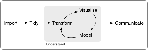
Figure 1: Process of data analysis.

Data analysis is the process of cleansing, transforming, and modeling data. The goal of data analysis is to derive meaningful and useful information from data. Fig. 1 shows the process of data analysis. The first step consists of gathering, importing and cleaning or tidying the data. Then the data is transformed and modeled to get some useful results [17]. Data analysis is used in almost every field of research. It is especially important in business intelligence and analytics. Business intelligence and analytics are data-driven approaches along with processes and tools for extracting information from data [18, 19, 20]. It helps businesses in making well-informed and efficient decisions [19, 21]. Data analytics offers a way of analyzing and extracting knowledge and useful insights from the data [19, 22]. Ayankoya et al. [23] explain the growing importance of data and data analysis, and the relation between data science, big data, and business analytics. Apart from business intelligence, data analysis is also used in various fields such as risk detection and management, healthcare [24, 25], security [26], transportation, and many other.

Data cleaning is the process of preparing data for analysis by removing or modifying incorrect, incomplete, irrelevant, duplicated, or improperly formatted data. This data is usually not necessary or helpful.Fig. 2 summarizes the process of data cleaning. Real world data is frequently dirty [27] and may contain imprecise values. The same comment is valid for the case with the financial fields [16]. There may be errors and impurities in the data, which should be filtered out before proceeding to the next steps in data analysis. These impurities can be caused by different factors, varying from faulty equipment, glitches in the systems used for recording observations or errors caused while storing data, to simply human errors. It is possible to reduce errors, but it is impossible to completely avoid them. Dirty time series data may contain impurities such as:

• Missing data

• Missing timestamps

• Outliers

• Duplicated observations

• Inconsistent data

• Problems with data types

• Problems with timestamp format, etc.

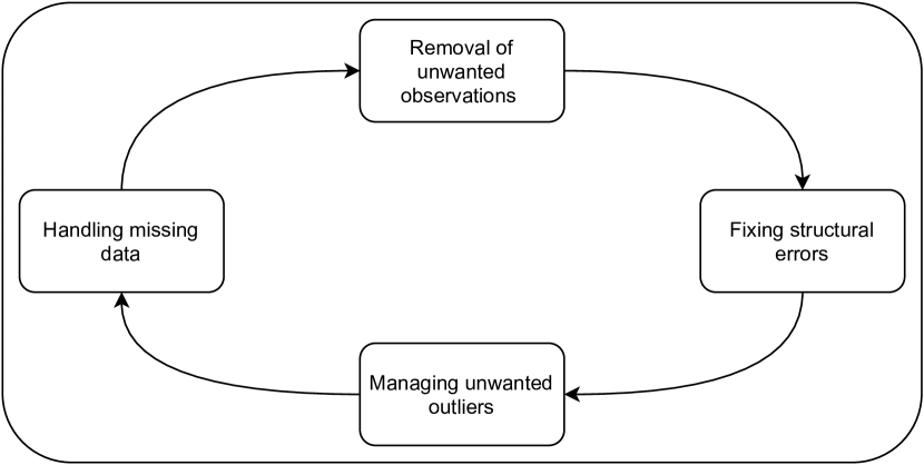
Figure 2: Data cleaning workflow.

2 Motivation

Data cleaning is the first step in the data analysis process. The results of all the other steps of the process depend on the results of data cleaning. Therefore, to get a proper analysis of the data it is crucial to clean it. The accuracy of many machine learning data analysis techniques and tools is heavily affected by the data. Many of such algorithms do not work on data containing missing values simply ignored. This may result in the loss of important data. The applications that are built upon unclean data are not reliable, such as pattern mining [28, 29] or classification [30]. Such data cannot be stored in a database, resulting in loss of data assets. Furthermore, the process of data cleaning is time-consuming and prone to human errors.

The previous sections of this study established the importance of data analysis and time series data cleaning. Therefore, data cleaning should be given great importance when performing data analysis. The data used is growing day by day. There are various tools available for the analysis of big data. Data cleaning and data visualization for such a large amount of data are particularly more challenging. Fig. 3 shows a time series containing 1,21,273 observations taken from Kaggle (https://www.kaggle.com/robikscube/hourly-energy-consumption). Since the number of observations is so high, the patterns in the plot are not visually clear. A subset of this plot is shown in Fig. 4, containing the data for a single month. Viewing the data in the weekly resolution makes it visually clear and more informative. This ensures the importance of analyzing the dataset at microscales. This is a part of the motivation in the visualization strategy for developing the proposed package, called cleanTS [31].

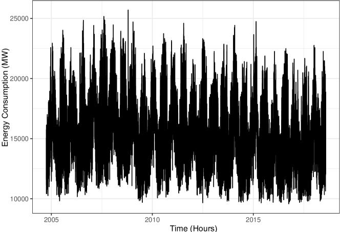
Figure 3: A sample time-series dataset.

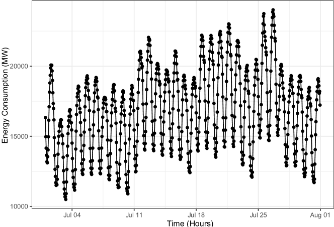
Figure 4: The first month in the dataset shown in Figure 3.

3 Literature Review

This section provides a review of state-of-the-art research contributions regarding the data cleaning process. Various tools available for the data cleaning process are discussed in this section. It also explains the concept of missing values, the importance of missing value imputation and several tools and algorithms that have been proposed in the literature and implemented for imputation of missing data.

It is a well established fact that dirty time series data can lead to unreliable and useless analytics, and in fact it has been previously commented. Therefore, data cleaning is the foremost task in the process of data analysis. The different problems that can arise in time series data cleaning are discussed in [16]. The amount of data and error rate during data collection is high. This is because sensors used to collect data are not always accurate. For example, in a steel mill, the surface temperature of the continuous casting slab cannot be accurately measured or may cause distortion due to the power of the sensor itself. Internet of Things (IoT) data is a common source of time series data. Karkouch et al. [32] explain the details of various IoT data errors generated by various complex environments. Most of the widely used time series cleaning methods utilize the principle of smooth filtering. Such methods may change the original data significantly, and result in the loss of the information contained in the original data. Data cleaning needs to avoid changing the original correct data, a process that should be based on the principle of minimum modification [33, 34, 35].

Table 1: State-of-the-art data cleaning tools.

Tool	Method	Description
Cleanits	Anomaly detection	Detects and repair the industrial time-series data. It considers the characteristics of the industrial time-series data and domain-specific knowledge for cleaning.
EDCleaner	Based on statistics	It works with data related to a social network. The detection and cleaning are performed through the characteristics of statistical data fields.
TsOutlier	Anomaly detection	Uses multiple algorithms to detect anomalies in time-series data, and supports both batch and streaming processing.
ASPA	Smoothing based	Automatically smooths streaming time series by adaptively optimizing the trade-off between noise reduction and trend retention.
PACAS	Based on statistics	Design a framework for data cleaning between service providers and customers.
PIClean	Based on statistics	Produces probabilistic errors and probabilistic fixes which help in implicitly discovering and using relationships between data columns for cleaning.
HoloClean	Based on statistics	Learn the probability model and select the data cleaning plan based on probability distribution.
ActiveClean	Based on statistics	Allows for progressive and iterative cleaning in statistical modeling problems.
MLClean	Anomaly detection	Combines data cleaning with machine learning methods.

Data cleaning is an important field for research and there have been various tools and systems proposed for it. Some of them have been listed in [16]. Ding et al. [36] propose an industrial time series cleaning system, Cleanits, which can detect and repair industrial time series. It provides a friendly interface so users can use results and logging visualization over every cleaning process. The algorithms used also take into consideration the characteristics of the industrial time series data and domain-specific knowledge. EDCleaner is proposed in [37] and works with data related to the social networks. The detection and cleaning are performed through the characteristics of statistical data fields. TsOutlier is a framework for detecting outliers presented in IoT data [38], that uses multiple algorithms to detect anomalies in time series data, and also supports batch and stream processing. The ASPA is a smoothing-based analytics operator that automatically smooths streaming time series by adaptively optimizing the trade-off between noise reduction and trend retention[39]. It violates the minimum modification principle and distorts the data, making it unsuitable for a wide use. PACAS [40] is a framework for data cleaning between service providers and customers. PIClean [41] is a statistics-based tool for cleaning. It produces probabilistic errors and probabilistic fixes which helps in implicitly discovering and using relationships between data columns for cleaning. HoloClean [42] selects the data cleaning plan based on probability distribution. ActiveClean [43] allows progressive and iterative cleaning in statistical modeling problems. MLClean [44] is an anomaly detection tool, which combines data cleaning with machine learning methods. Table 1 lists all the mentioned tools.

The problem of missing data arises frequently and is very common. A lot of research has been done in the field of imputation. Almost whenever data is recorded, problems regarding missing values occur. There are different reasons for the absence of an observation, such as not measured or lost values or values that have been finally considered not valid [45]. There are three missing data mechanisms, discussed in [45]:

• Missing completely at random (MCAR): In MCAR there is no systematic mechanism on the way the data is missing. The occurrence of missing data points is completely random. This means that in univariate time series data, the probability of the observation to be missed does not depend on the time the observation is recorded.

• Missing at random (MAR): In MAR the probability of missed observation does not depend on the value of the observation itself, but on other variables. As pointed out in [45], the majority of missing data methods require MAR or MCAR. The MAR mechanism allows the imputation algorithms to use correlations with other variables, so better results compared to MCAR can be obtained.

• Not missing at random (NMAR): In NMAR, the data points are not missing at random. The probability of a missed value depends on the value of the observation, and can also be dependent on other variables. NMAR is called non-ignorable because in order to perform the imputation, a special model for why data is missing and what the likely values are, needs to be included.

There are various algorithms and packages in the R programming language to deal with missing data. Some of these ar, imputation based on random forests [46], nearest neighbor observation [47], predictive mean matching [48], maximum likelihood estimation [49], conditional copula specifications [50], expectation-maximization [51]. [52] and [53] provide various algorithms and tools for imputation.

An anomaly or an outlier is a recorded observation in a time series data, which is significantly different from other observations. Such an observation deviates too much from other ones. They are also called abnormalities, deviants and discordants [54, 55]. Outlier detection is very useful and important in many areas like intrusion detection, credit-card fraud, medical diagnosis, earth science, law enforcement and many more. Anomaly detection is also very important in data analysis. It is possible that a data point which represents an anomaly may be an error while recording the observation, i.e, it is an invalid data point. Such invalid data points are not desirable for data analysis, since they can significantly affect the data analysis results. But it is also possible that the data point is correct. If it is in fact an error, then it is important to remove it from the data before analyzing the data.

4 Introduction to R Package cleanTS

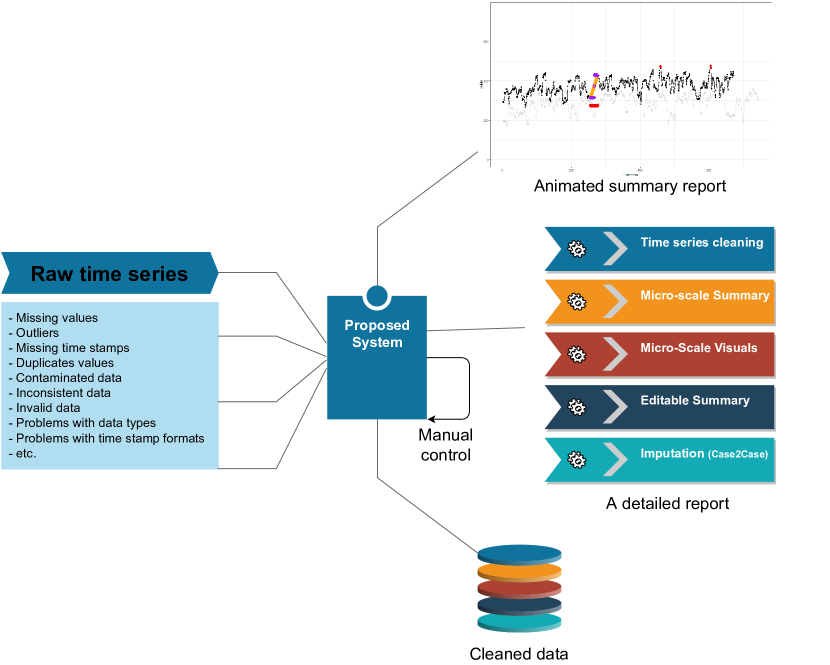
Figure 5: Worflow of the proposed system.

This package focuses on the development of a tool that makes the process of cleaning large datasets simple and time-efficient. It implements reliable and efficient procedures for automating the process of cleaning univariate time series data. The time required for cleaning the data is significantly reduced if the process is automated. The tool provides integration with already developed and deployed tools for missing value imputation. The main problem with visualizing large amounts of data is that the visualizations are not very informative. The tool provides a way of visualizing large time series data in different resolutions. It is intended to be used by researchers from various domains, who want to work on data-science-related projects. Gateways and procedures are also included in the tool, for the researchers who are interested in using the proposed tool for introducing and adding new methodologies and algorithms in the domain. Figure  5 contains a brief summary of the proposed system. The tool is designed such that it requires minimum user interaction. The ultimate goal is the creation of a handy software tool that deals with all the problems, processes, analysis, and visualization of big data time series, with or without human intervention.

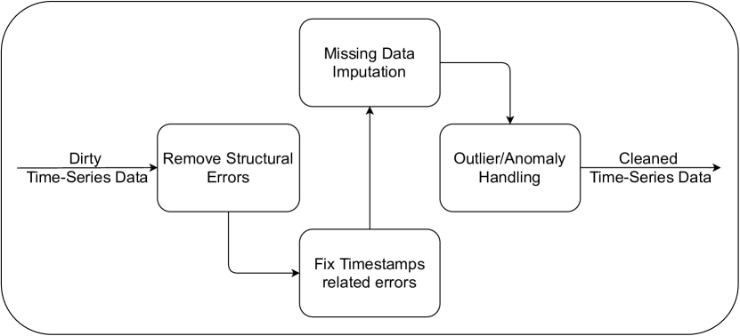
Figure 6: Flowchart for the proposed system.

Figures 5 and 6 show the workflow of the system. The system requires univariate time series data as input. Data cleaning of multivariate time series and non-time series data is out of the scope of the present version of the tool. Section 1 listed the impurities that may be present in the time series data. The system has procedures implemented to handle each of these impurities. After the impurities have been removed or corrected, it generates a detailed report on the entire process, notifying the user of all the changes to make to the original data. This report allows the users to review the changes and revert them make if required. The system also provides a tool for visualizing the data in different resolutions. These procedures generate an animated visualization or an interactive plot, which helps with the micro-scale visualization and analysis of the data.

R is a programming language specifically designed to be used for statistical computing and graphical visualization [56]. The graphics tools provided by R are one of the best for data analysis and display either on-screen or on hardcopy. There are many efficient and reliable tools for performing any task related to data science, such as data wrangling, data visualization, machine learning, etc. These packages are updated and maintained regularly. The proposed system is implemented in the R programming language. This section provides details on each function in the package. All the functions available to the users are listed in Table 2. Each of the data cleaning tasks is divided into internal functions. Several other internal helper functions are not intended to be used directly by the user and hence are not listed here.

In R there are various libraries used for data manipulation, data wrangling, and working with data in general. Two such libraries are the data.table package [57] and the tidyverse family of packages [58]. The tidyverse is a collection of packages for solving data science challenges using R code. Some of the packages in tidyverse includes dplyr[59], tibble[60], ggplot2[61] and tidyr[62]. They are user-friendly, efficient, and share the same design methodology. Also, the code written with these packages is clean and easily understandable. The data.table provides a high-performance version of base R’s data.frame. It is useful for tasks such as aggregating, filtering, merging, grouping, and other related tasks. Both of these packages are a lot faster than their base R equivalents. When considering data.table and dplyr, it can be seen that data.table gets faster than dplyr as the number of groups and/or rows to group increase [63]. Since the proposed tool needs to work with a large amount of data, the R package uses the data.table backend.

4.1 Highlights

1. Automation of data cleaning: Primarily, the package automates the cleaning and organizing the process of cleaning big (voluminous) time series data. It includes fixing structural errors, timestamp related errors, and handling missing values and anomalies in the data. The process of univariate time series cleaning is discussed in detail in Section 1.

2. Integrated with imputation tools: There are various tools, available for the automation of missing value imputation. These tools are already tested and deployed. The cleanTS package makes use of such tools for handling missing value imputation in univariate time series data. One such package used is the imputeTestbench package, which provides a benchmarking tool for comparing various methods of imputation. It is also possible to add new imputation methodology and algorithms and compare them to existing once. This integration has enabled the creation of a handy software tool that deal with the pre-processing, analysis and visualization of big data time series with minimum to no human intervention.

3. Graphical user-interface: The tool is targeted towards researchers working in several domains and willing to work on data science related projects in their respective domains with an interactive tool. It provides a user-friendly and easy to understand GUI (graphical user-interface). This enables the tool to be used by the users with no coding knowledge or experience.

4. Micro scale visualization:The package provides procedures and functions for visualizing the time series data at micro scales. It involves splitting the data according to the provided interval and then creating the visualization for each part of the data. This tool analyzes the time series at the micro-level and assists in cleaning it in an interactive manner with data science principles.

4.2 Installation

The cleanTS package can be installed from github.

    # Install from GitHub

    install.packages("devtools")

    devtools::install_github("Mayur1009/cleanTS")

    # Install from CRAN

    install.packages("cleanTS")

The system on which the package is to be installed needs to have R and RStudio installed on the machine. On a Windows machine, this setup is enough to install the package, but on Linux-based systems like Ubuntu, some extra packages are required. For the installation of the gganimate package a Rust compiler is required. This can be installed by using, sudo apt-get install cargo on Debian/Ubuntu, yum install cargo on Fedora/CentOS, brew install rustc on MacOS.

4.3 Functions and Implementation Methodology

Table 2: Functions in cleanTS package.

Functions	Description
cleanTS()	Function for cleaning the input data. It creates and returns a cleanTS object.
gen.report()	Generates a report of the process of data cleaning, from the given ‘cleanTS‘ object.
animate_interval()	Create an animated plot from the given cleanTS object and a specified interval.
gen.animation()	Renders the animation using a gganim object returned by animate_interval().
interact_plot()	Creates an interactive plot from the given cleanTS object and a specified interval.

1. cleanTS()

   cleanTS(data, date_format, imp_methods = c("na_interpolation",

   "na_locf", "na_ma", "na_kalman"), time = NULL, value = NULL,

   replace_outliers = T)

   • data: The input time series data. Can be a data.frame, tbl, or table-like object.

   • date_format: A character string, the format of the time column in the data.

   • imp_methods: A vector of strings, the methods of imputation to be used for imputing missing values. The default value specifies four methods, na_interpolation, na_locf, na_ma, na_kalman.

   • time: Name of the column containing timestamps. If NULL the first column is considered to be the time column.

   • value: Name of the column containing observations. If NULL the second column is considered to be the time column.

   • replace_outliers: Defaults to TRUE. Specify whether to remove and impute the detected outliers in the time series.

   cleanTS() is the entry function to the package. It is a wrapper function that calls all the other internal functions to performs different data cleaning tasks. The first task is to check the input time series data for structural and data type-related errors. Since the functions need univariate time series data, the input data is checked for the number of columns. By default, the first column is considered to be the time column, and the second column to be the observations. Alternatively, if the time and value arguments are given, then those columns are used. The time column is converted to a POSIX object using the lubridate package [64]. Lubridate allows the format to be specified in a very easy and simplified way. A complete list of all the possible date-time formats is provides in [65]. The value column is converted to a numeric type. If it contains invalid data, like a string of random characters, which cannot be parsed to numeric, they are replaced with NA. The column names are also changed to time and value. All the data is converted to a data.table object. This data is then passed to other functions to check for missing and duplicate timestamps. If there are any missing timestamps found, they are inserted in the data and the corresponding observations are set to NA. If duplicate timestamps are found, then the observation values are checked. If the observations are the same, then only one copy of that observation is kept. But if the observations are different, then it is not possible to find the correct one, so the observation is set to NA.

   This data is then passed to a function for finding and handling missing observations. These are represented by NA in the value column of the data. The problem of missing data arises frequently and is very common. A lot of research has been done in the field of imputation, which has been discussed in Section 3. The package provides integration with the imputeTestbench package [66, 67]. It provides the function for comparing various methods of imputation. Using these functions the methods given in the imp_methods argument are compared and selected. The imputeTestbench also offers functionality to separately find the best methods for MCAR and MAR types of missing values. After the best methods are found, imputation is performed using those methods. The user can also pass user-defined functions for comparison. The default functions are provided by the imputeTS package [68]. It provides functions for imputation by linear interpolation, imputation by structural model and Kalman smoothing, imputation by last observation carried forward, imputation by simple moving average, imputation by mean value, and many more. The user-defined function should follow the structure as the default functions. It should take a numeric vector containing missing values as input, and return a numeric vector of the same length without missing values as output.

   Once the missing values are handled the data is checked for outliers. The anomalize package [69] provides great functions for finding outliers/anomalies in time series data. The anomalize package accepts only tibble (class tbl_df) [60] or tibbletime (class tbl_time) [70] objects. The tibbletime is an extension of tibble that creates time-aware tibbles by setting a time index. The general workflow for anomaly detection includes the decomposition of the time series data into the seasonal, trend, and remainder components, then applying anomaly detection on the remainder part. This generates the lower and upper limits for the data. Any observation outside these limits is treated as an outlier or anomaly. If the replace_outliers parameter is set to TRUE in the cleanTS() function, then the outliers are replaced by NA and imputed using the procedure mentioned for imputing missing values. Then it creates a cleanTS object which contains the cleaned data, missing timestamps, duplicate timestamps, imputation methods, MCAR imputation error, MAR imputation error, outliers, and if the outliers are replaced then imputation errors for those imputations are also included. The cleanTS object is returned by the function.
   

2. gen.report()

   gen.report(obj)

   • obj: The cleanTS object, returned by the cleanTS() function.

   The cleanTS() function handles all the data cleaning tasks. It makes a lot of changes to the original data. The gen.report() function shows a report of these changes and gives details about the impurities found in the data.
   

3. animate_interval()

   animate_interval(obj, interval)

   • obj: The cleanTS object, returned by the cleanTS() function.

   • interval: A string or numeric value, specifying the viewing resolution in the plot.

   animate_interval() creates an animated plot for the given data. First, the data is split according to the interval. If it is a numeric value, the cleaned data is split into dataframes containing interval observations. It can also be a string, like 1 week, 3 months, 14 days, etc. In this case, the data is split according to the interval given. The gganimate package [71] is an extension of the ggplot2 library [61], which adds functionality to animate the plot. Here we split the data into states according to the given interval and then use transition_state() function from gganimate. The animate_interval() function returns a list containing the gganim object used to generate the animation and the number of states in the data. The animation can be generated using the gen.animation() function and saved using the anim_save() function. The plots in the animation also contain a short summary, containing the statistical information and the number of missing values, outliers, missing timestamps, and duplicate timestamps in the data shown in that frame of animation.
   

4. gen.animation()

   gen.animation(anim, nframes = 2 * anim$nstates,

   duration = anim$nstate, ...)

   • anim: A list containing a gganim object and number of states (numeric).

   • nframes: The number of frames to render in the animation.

   • duration: The duration of the generated animation.

   • ... : Other arguments passed to animate() function in the gganimate package.

   gen.animation() is a simple wrapper function for the animate() function which is used to render the animation using a gganim object. By default, in the animate() function only 50 states in the data are shown. So, to avoid this gen.animation() defines the default value for the number of frames. Also, the duration argument has a default value equal to the number of states, making the animation slower. More arguments can be passed, which are then passed to animate(), like, height, width, fps, renderer, etc.
   

5. interact_plot()

   interact_plot(obj, interval)

   • obj: The cleanTS object, returned by the cleanTS() function.

   • interval: A string or numeric value, specifying the viewing resolution in the plot.

   The problem with an animated plot is that the user does not have any control over the animation. There is not play or pause functionality so that the user can observe any desired frame. This can be achieved by adding interactivity to the plot. In the R programming language, shiny [72] provides a web application framework. It is an R package that creates interactive web apps using R. The interact_plot() function creates and runs a shiny widget locally on the machine. It takes the cleanTS object and splits the cleaned data according to the interval argument, similar to the animate_interval() function. It then creates a shiny widget which shows the plot for the current state and gives a slider used to change the state. Unlike animate_interval() it provides a global report containing information about complete data, and a state report giving information about the current state shown in the plot.
   

6. mergecsv()

   mergecsv(path, formats)

   • path: The path to the folder containing the CSV files to merge.

   • formats: The format of the timestamps used in the CSV files.

   The mergecsv() function reads the CSV files found in the given path. It is assumed that in each CSV the first column contains the timestamps. All these files are read and the first column is parsed to a proper DateTime object using the formats given in the formats argument. Then these dataframes are merged using the timestamp column as a common column. The merged data frame returned by the function contains the first column as the timestamps. The Appendix A demonstrates the working of this function with an example.
   

4.4 The cleanTS Web Application

One of the requirements for using the package is having the R programming language installed on a local machine. Also, one needs to have at least some basic coding knowledge and experience to use the package. These drawbacks can be avoided using a web-based application, that runs on a web server and is accessed through a web browser. The user does not need to have R installed on their local systems. This enables users without any programming knowledge, to use the cleanTS tool. The cleanTS web app is created using shiny, available at https://mayur1009.shinyapps.io/cleanTS/. The user needs to upload a CSV file containing the data and enter the format of the timestamps used in the data. The uploaded data and the statistical information of the data are calculated and displayed. The user then needs to select the imputation methods and press the start button. It is possible to add imputation methods by uploading an R source file containing the function. Once the data is cleaned, it is displayed along with its statistical information. The user can then download the cleaned data as a CSV file. The app also created an interactive plot for micro-scale visualization of the data. The plot can be converted to a GIF file and downloaded.

5 Results and Conclusion

Time series are used in a lot of different fields ranging from biology to social science and industries. The time series data is usually collected using sensors, which are prone to making errors and malfunctioning. These errors in data make the analytics unreliable. Bad analytics can greatly affect decision-making in businesses. Because the error rates are high, it has become very important to clean the time series data before using it. Also, it is found that data cleaning is a cumbersome task, especially in cases where the data is very large. A lot of time is consumed by the data cleaning process.

There are various tools developed for cleaning data, as discussed in the literature review of this paper. But many of these proposed tools are designed to operate on data for a specific field. Furthermore, many of them are not specifically designed for univariate time series data. A significant amount of research has been done related to missing value imputation. Missing data is a very common problem in real-world datasets, especially the ones recorded using sensors. Section 3 discusses the various mechanisms of missing data. It also focuses on various tools and algorithms for missing data imputation.

This paper proposed a tool that automates the process of data cleaning for univariate time series data. The working and the implementation of the tool is also explained in detail. Firstly, the tool fixes any structural and datatype related errors. Then the timestamps of the data are observed for any missing timestamps or duplicate timestamps. Once the timestamps are fixed, missing values and anomalies or outliers in the data are handled. The tool also provides functions for visualizing the data in different resolutions. Section Illustrative Examples of this paper takes three different datasets to demonstrate the working of the proposed tool. Since the output plots generated are animated and interactive, they cannot be shown here.

Table 3: Measuring the running time of cleanTS function.

Data	Min	Lower Qrtl.	Mean	Median	Upper Qrtl.	Max	unit
Power Consumption Dataset	19.99	20.87	21.66	21.57	22.29	24.59	sec
CO2 Emission Dataset	194.90	198.70	203.50	199.90	210.49	226.67	msec
Temperature Dataset	13.49	14.18	14.38	14.42	14.56	15.10	sec

The performance metric for the three datasets Power consumption, CO₂ emission, and temperature are listed in Table 3. The power consumption dataset is very large and contains 121,273 observations. The CO₂ emission contains 1392 observations and the temperature dataset contains 45,253 observations. To evaluate the running time shown in Table 3, the microbenchmark package [73] was used. From the examples shown in Section Illustrative Examples, it can be found that the package is user-friendly and easy to use. Also, the testing results show that the package is efficient and works well with a large amount of data. As of writing this paper, the package only works with univariate time series data, but it can be extended to work with multivariate datasets. Also, the package can be integrated to work with big data and databases by integration with Apache Spark. The package already works relatively well with a huge amount of data, but more efficiency can be achieved in future.

5.1 Future Scope

One of the limitations of the proposed package is that it only works with an univariate time series data. But it might be possible to add functionality that supports multivariate data, or even non-time series data. As of writing this article, the package uses the data.table library for working with the data. This is far more reliable and efficient at handling huge amounts of data than the base R dataframes. But it might be possible to integrate it with Apache Spark, to work with Big Data. It is also a worthwhile to investigate the possibility of adding parallel computing to make it faster.

The tool will be modified for DNA and RNA sequencing applications, which have the potential to ease various processes involved in genetics and bioinformatics projects and experiments.

A major application of this tool will be in environmental datasets processing and analysis. The usability of the proposed tool and its GUI will be demonstrated for real-time energy market applications, which will automatically capture the time series, clean and organize it, analyze it and estimate the forecast with the least possible error and generate a detailed report.

Appendix A

This Appendix explains and gives an example for the mergecsv() function, explained in section 6. We have four CSV files in the CSVFiles folder. The first column of each of these files contains the timestamps. The formats argument contains a list of timestamp formats expected to be found while parsing the timestamp columns.

# Combine the csv files in the `CSVfiles` folder

merged <- mergecsv(path = "CSVFiles/",

                    formats = c("dmyHMs", "ymdHMS"))

# Write the merged dataframe to `mergeCSV.csv` file

data.table::fwrite(merged, "mergedCSV.csv")

After the files are merged, the function returns a data.table, which can then be written to a CSV file using the write.csv() function or the data.table::fwrite() function.

Illustrative Examples

Hourly Power Consumption

The data set used below is taken from Kaggle [74]. It contains over 10 years of hourly energy consumption data from 1st October 2004 to 3rd August 2018. The data is taken from PJM’s website. PJM Interconnection LLC (PJM) is a regional transmission organization (RTO) in the United States. The hourly consumption data is recorded in megawatts(MW). There are 1,21,273 observations recorded in the dataset. The statistical information about the data is given in Table 4.

# Load the hourly data consumption data

data <- data.table::fread("data/AEP_hourly.csv")

summary(data)

##     Datetime                       AEP_MW
##  Min.   :2004-10-01 01:00:00   Min.   : 9581
##  1st Qu.:2008-03-17 15:00:00   1st Qu.:13630
##  Median :2011-09-02 04:00:00   Median :15310
##  Mean   :2011-09-02 03:17:01   Mean   :15500
##  3rd Qu.:2015-02-16 17:00:00   3rd Qu.:17200
##  Max.   :2018-08-03 00:00:00   Max.   :25695

Table 4: Statistical information of the Hourly consumption dataset.

Min.	1st Qu.	Median	Mean	3rd Qu.	Max.
9581	13630	15310	15499.51	17200	25695

# Load the cleanTS library

library(cleanTS)

# Use the `cleanTS()` function for cleaning the data.

cts <- cleanTS(data = data, date_format = "ymdHMs",

    replace_outliers = T)

# The `cleanTS()` function returns a cleanTS object.

summary(cts)

##                  Length Class      Mode
## clean_data        5     data.table list
## missing_ts       27     POSIXct    numeric
## duplicate_ts      4     POSIXct    numeric
## imp_methods       4     -none-     character
## mcar_err          4     data.frame list
## mar_err           0     data.frame list
## outliers          4     data.table list
## outlier_mcar_err  4     data.frame list
## outlier_mar_err   4     data.frame list

# Print the cleanTS object

print(cts)

## $clean_data
## # A tibble: 121,296 x 5
##    time                value missing_type method_used is_outlier
##    <dttm>              <dbl> <chr>        <chr>       <lgl>
##  1 2004-10-01 01:00:00 12379 <NA>         <NA>        FALSE
##  2 2004-10-01 02:00:00 11935 <NA>         <NA>        FALSE
##  3 2004-10-01 03:00:00 11692 <NA>         <NA>        FALSE
##  4 2004-10-01 04:00:00 11597 <NA>         <NA>        FALSE
##  5 2004-10-01 05:00:00 11681 <NA>         <NA>        FALSE
##  6 2004-10-01 06:00:00 12280 <NA>         <NA>        FALSE
##  7 2004-10-01 07:00:00 13692 <NA>         <NA>        FALSE
##  8 2004-10-01 08:00:00 14618 <NA>         <NA>        FALSE
##  9 2004-10-01 09:00:00 14903 <NA>         <NA>        FALSE
## 10 2004-10-01 10:00:00 15118 <NA>         <NA>        FALSE
## # ... with 121,286 more rows
##
## $missing_ts
##  [1] "2004-10-31 02:00:00 UTC" "2005-04-03 03:00:00 UTC"
##  [3] "2005-10-30 02:00:00 UTC" "2006-04-02 03:00:00 UTC"
##  [5] "2006-10-29 02:00:00 UTC" "2007-03-11 03:00:00 UTC"
##  [7] "2007-11-04 02:00:00 UTC" "2008-03-09 03:00:00 UTC"
##  [9] "2008-11-02 02:00:00 UTC" "2009-03-08 03:00:00 UTC"
## [11] "2009-11-01 02:00:00 UTC" "2010-03-14 03:00:00 UTC"
## [13] "2010-11-07 02:00:00 UTC" "2010-12-10 00:00:00 UTC"
## [15] "2011-03-13 03:00:00 UTC" "2011-11-06 02:00:00 UTC"
## [17] "2012-03-11 03:00:00 UTC" "2012-11-04 02:00:00 UTC"
## [19] "2012-12-06 04:00:00 UTC" "2013-03-10 03:00:00 UTC"
## [21] "2013-11-03 02:00:00 UTC" "2014-03-09 03:00:00 UTC"
## [23] "2014-03-11 14:00:00 UTC" "2015-03-08 03:00:00 UTC"
## [25] "2016-03-13 03:00:00 UTC" "2017-03-12 03:00:00 UTC"
## [27] "2018-03-11 03:00:00 UTC"
##
## $duplicate_ts
## [1] "2014-11-02 02:00:00 UTC" "2015-11-01 02:00:00 UTC"
## [3] "2016-11-06 02:00:00 UTC" "2017-11-05 02:00:00 UTC"
##
## $imp_methods
## [1] "na_interpolation, na_locf, na_ma, na_kalman"
##
## $mcar_err
## # A tibble: 1 x 4
##   na_interpolation na_locf na_ma na_kalman
##              <dbl>   <dbl> <dbl>     <dbl>
## 1             2.84    9.17  6.45      1.84
##
## $mar_err
## # A tibble: 0 x 0
##
## $outliers
## # A tibble: 38 x 4
##    time                 value orig_value method_used
##    <dttm>               <dbl>      <dbl> <chr>
##  1 2006-05-30 16:00:00 22113.      22011 na_kalman
##  2 2006-05-30 17:00:00 22102.      22119 na_kalman
##  3 2007-07-09 15:00:00 23984.      23818 na_kalman
##  4 2007-07-09 16:00:00 24229.      23940 na_kalman
##  5 2007-07-09 17:00:00 24236.      24038 na_kalman
##  6 2007-08-23 16:00:00 24974.      24828 na_kalman
##  7 2007-08-23 17:00:00 24984.      24862 na_kalman
##  8 2008-06-09 15:00:00 24077.      23938 na_kalman
##  9 2008-06-09 16:00:00 24145.      23828 na_kalman
## 10 2008-06-09 17:00:00 24005.      23900 na_kalman
## # ... with 28 more rows
##
## $outlier_mcar_err
## # A tibble: 1 x 4
##   na_interpolation na_locf na_ma na_kalman
##              <dbl>   <dbl> <dbl>     <dbl>
## 1            0.726    2.67  1.97     0.340
##
## $outlier_mar_err
## # A tibble: 1 x 4
##   na_interpolation na_locf na_ma na_kalman
##              <dbl>   <dbl> <dbl>     <dbl>
## 1             30.6    43.2  32.1      27.3

# Use the `gen.report()` function to get a detailed report.

gen.report(cts)

##
## # Summary of cleaned data:
##    Min. 1st Qu.  Median    Mean 3rd Qu.    Max.
##    9581   13629   15309   15499   17200   25164
##
## # Missing timestamps:  27
##  [1] "2004-10-31 02:00:00 UTC" "2005-04-03 03:00:00 UTC"
##  [3] "2005-10-30 02:00:00 UTC" "2006-04-02 03:00:00 UTC"
##  [5] "2006-10-29 02:00:00 UTC" "2007-03-11 03:00:00 UTC"
##  [7] "2007-11-04 02:00:00 UTC" "2008-03-09 03:00:00 UTC"
##  [9] "2008-11-02 02:00:00 UTC" "2009-03-08 03:00:00 UTC"
## [11] "2009-11-01 02:00:00 UTC" "2010-03-14 03:00:00 UTC"
## [13] "2010-11-07 02:00:00 UTC" "2010-12-10 00:00:00 UTC"
## [15] "2011-03-13 03:00:00 UTC" "2011-11-06 02:00:00 UTC"
## [17] "2012-03-11 03:00:00 UTC" "2012-11-04 02:00:00 UTC"
## [19] "2012-12-06 04:00:00 UTC" "2013-03-10 03:00:00 UTC"
## [21] "2013-11-03 02:00:00 UTC" "2014-03-09 03:00:00 UTC"
## [23] "2014-03-11 14:00:00 UTC" "2015-03-08 03:00:00 UTC"
## [25] "2016-03-13 03:00:00 UTC" "2017-03-12 03:00:00 UTC"
## [27] "2018-03-11 03:00:00 UTC"
##
## # Duplicate timestamps:  0
##
## No duplicate timestamps found.
##
## # Missing Values:  31 (0.0255573143384778%)
##
## ## MCAR:  31 (0.0255573143384778%)
##  MCAR Errors:
##   na_interpolation  na_locf    na_ma na_kalman
## 1         2.844675 9.173093 6.446093  1.836841
##
##                    time    value method_used
##  1: 2004-10-31 02:00:00 10759.00   na_kalman
##  2: 2005-04-03 03:00:00 13334.83   na_kalman
##  3: 2005-10-30 02:00:00 13158.50   na_kalman
##  4: 2006-04-02 03:00:00 11234.17   na_kalman
##  5: 2006-10-29 02:00:00 13128.33   na_kalman
##  6: 2007-03-11 03:00:00 13017.33   na_kalman
##  7: 2007-11-04 02:00:00 13347.50   na_kalman
##  8: 2008-03-09 03:00:00 17156.83   na_kalman
##  9: 2008-11-02 02:00:00 12292.50   na_kalman
## 10: 2009-03-08 03:00:00 10991.67   na_kalman
## 11: 2009-11-01 02:00:00 11551.00   na_kalman
## 12: 2010-03-14 03:00:00 12546.00   na_kalman
## 13: 2010-11-07 02:00:00 14467.67   na_kalman
## 14: 2010-12-10 00:00:00 18107.33   na_kalman
## 15: 2011-03-13 03:00:00 12787.83   na_kalman
## 16: 2011-11-06 02:00:00 13279.33   na_kalman
## 17: 2012-03-11 03:00:00 13397.50   na_kalman
## 18: 2012-11-04 02:00:00 12432.17   na_kalman
## 19: 2012-12-06 04:00:00 14801.50   na_kalman
## 20: 2013-03-10 03:00:00 12429.83   na_kalman
## 21: 2013-11-03 02:00:00 11713.33   na_kalman
## 22: 2014-03-09 03:00:00 13021.00   na_kalman
## 23: 2014-03-11 14:00:00 14635.33   na_kalman
## 24: 2014-11-02 02:00:00 12952.17   na_kalman
## 25: 2015-03-08 03:00:00 14044.50   na_kalman
## 26: 2015-11-01 02:00:00 10695.50   na_kalman
## 27: 2016-03-13 03:00:00 10218.17   na_kalman
## 28: 2016-11-06 02:00:00 11049.83   na_kalman
## 29: 2017-03-12 03:00:00 14301.83   na_kalman
## 30: 2017-11-05 02:00:00 10535.67   na_kalman
## 31: 2018-03-11 03:00:00 13722.17   na_kalman
##                    time    value method_used
##
##
## ## MAR:  0 (0%)
## No MAR found.
##
## # Outliers:  38
##                    time    value orig_value method_used
##  1: 2006-05-30 16:00:00 22112.80      22011   na_kalman
##  2: 2006-05-30 17:00:00 22101.70      22119   na_kalman
##  3: 2007-07-09 15:00:00 23984.40      23818   na_kalman
##  4: 2007-07-09 16:00:00 24228.80      23940   na_kalman
##  5: 2007-07-09 17:00:00 24235.80      24038   na_kalman
##  6: 2007-08-23 16:00:00 24974.40      24828   na_kalman
##  7: 2007-08-23 17:00:00 24984.10      24862   na_kalman
##  8: 2008-06-09 15:00:00 24077.40      23938   na_kalman
##  9: 2008-06-09 16:00:00 24145.30      23828   na_kalman
## 10: 2008-06-09 17:00:00 24004.80      23900   na_kalman
## 11: 2008-10-20 14:00:00 16174.83      25695   na_kalman
## 12: 2009-03-03 07:00:00 21756.17      22068   na_kalman
## 13: 2010-08-30 16:00:00 22847.60      22777   na_kalman
## 14: 2010-08-30 17:00:00 22898.40      22958   na_kalman
## 15: 2010-08-31 16:00:00 22789.80      22839   na_kalman
## 16: 2010-08-31 17:00:00 22989.20      23023   na_kalman
## 17: 2011-09-02 15:00:00 22741.00      22666   na_kalman
## 18: 2011-09-02 16:00:00 22967.00      22826   na_kalman
## 19: 2011-09-02 17:00:00 22899.00      22893   na_kalman
## 20: 2012-06-30 08:00:00 10021.30      10015   na_kalman
## 21: 2012-06-30 09:00:00 10588.20      10582   na_kalman
## 22: 2013-09-10 14:00:00 21876.21      22016   na_kalman
## 23: 2013-09-10 15:00:00 22391.00      22631   na_kalman
## 24: 2013-09-10 16:00:00 22630.71      22781   na_kalman
## 25: 2013-09-10 17:00:00 22611.71      22722   na_kalman
## 26: 2013-09-10 18:00:00 22350.36      22433   na_kalman
## 27: 2014-01-07 01:00:00 21879.29      21807   na_kalman
## 28: 2014-01-07 02:00:00 21893.30      21684   na_kalman
## 29: 2014-01-07 03:00:00 22048.44      21689   na_kalman
## 30: 2014-01-07 04:00:00 22300.15      21785   na_kalman
## 31: 2014-01-07 05:00:00 22603.85      21892   na_kalman
## 32: 2014-01-07 06:00:00 22914.96      22278   na_kalman
## 33: 2014-01-07 07:00:00 23188.90      23076   na_kalman
## 34: 2014-01-07 08:00:00 23381.11      23590   na_kalman
## 35: 2015-01-08 05:00:00 21587.60      21435   na_kalman
## 36: 2015-01-08 06:00:00 22393.90      22182   na_kalman
## 37: 2015-01-08 07:00:00 23173.00      23056   na_kalman
## 38: 2015-02-20 06:00:00 23397.83      23412   na_kalman
##                    time    value orig_value method_used
## ## Imputation errors while replacing outliers:
## ### MCAR errors:
##   na_interpolation  na_locf    na_ma na_kalman
## 1        0.7262274 2.670749 1.974189 0.3398252
## ### MAR errors:
##   na_interpolation  na_locf    na_ma na_kalman
## 1         30.59071 43.16642 32.12617  27.31822

# Use the `animate_interval()` function to create a animation

# object.

anim <- animate_interval(cts, interval = "1 month")

# The animation is generated using `gen.animation()` function.

gen.animation(anim)

# This animation can be saved using `anim_save()` function.

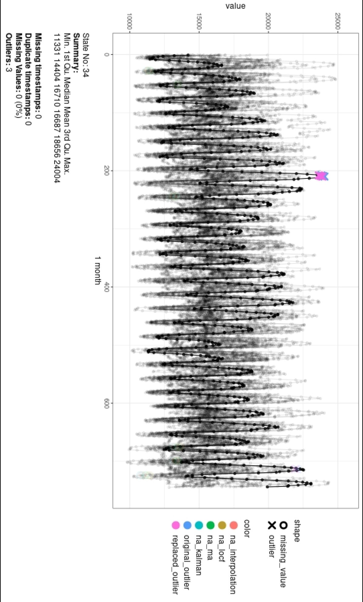
Figure 7: A state from the animated plot generated for Example 1

# Start a interactive plot using the `interact_plot()`

# function.

interact_plot(cts, interval = "1 month")

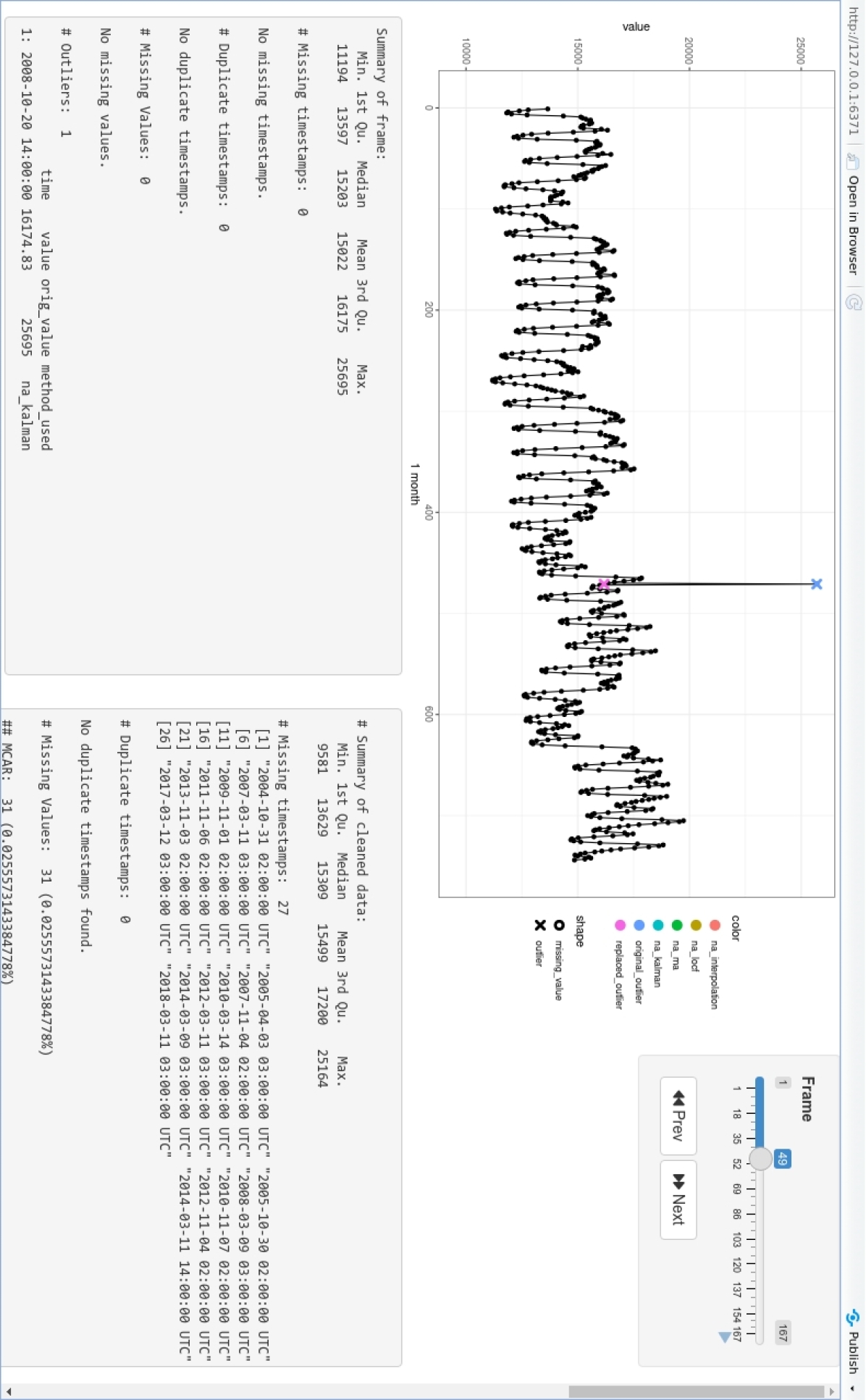
Figure 8: A state from the interactive plot generated for Example 1

Figure 7 and Figure 8 shows a single state from the animated and interactive plots respectively.

Carbon-dioxide Emission

For this example, the CO2 emission dataset is used. This dataset was used in [75, 76], for short-term CO₂ emission forecasting. Data is used from the ENSTO-E transparency platform for 2018 and 2019. The dataset contains the electricity generation per technology, electricity demand per price area, as well as power, flows between interconnected areas. The flow tracing is used to map the power flows between importing and exporting countries. The country-specific average CO₂ emission intensity per generation technology is applied to the flow tracing results to calculate the hourly CO₂ intensity of electricity consumption for each price area. The statistical information for this dataset is shown in Table 5. Figure 9 shows the plot for the dataset.

Table 5: Statistical information of the CO2 emission dataset.

Min.	1st Qu.	Median	Mean	3rd Qu.	Max.
270.23	370.46	402.545	405.9396	437.5025	542.06

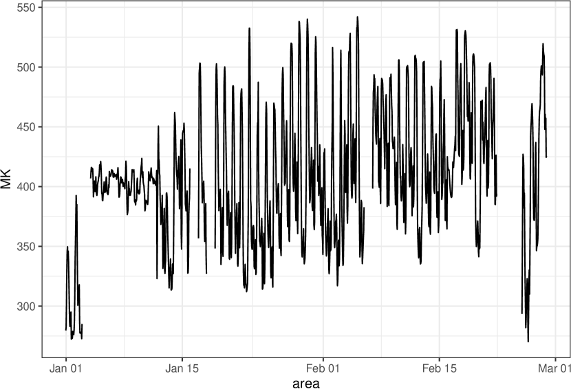
Figure 9: Plot for the CO2 emission dataset

# Load the hourly data consumption data

data <- data.table::fread("data/co2dat.csv")

summary(data)

##       area                           MK
##  Min.   :2016-12-31 23:00:00   Min.   :270.2
##  1st Qu.:2017-01-15 10:45:00   1st Qu.:370.5
##  Median :2017-01-29 22:30:00   Median :402.5
##  Mean   :2017-01-29 22:30:00   Mean   :405.9
##  3rd Qu.:2017-02-13 10:15:00   3rd Qu.:437.5
##  Max.   :2017-02-27 22:00:00   Max.   :542.1
##                                NA’s   :168

# Load the cleanTS library

library(cleanTS)

# Use the `cleanTS()` function for

# cleaning the data.

cts <- cleanTS(data = data, date_format = "ymdHMs",

    replace_outliers = T)

# The `cleanTS()` function returns a cleanTS object.

summary(cts)

##                  Length Class      Mode
## clean_data       5      data.table list
## missing_ts       0      POSIXct    numeric
## duplicate_ts     0      POSIXct    numeric
## imp_methods      4      -none-     character
## mcar_err         0      data.frame list
## mar_err          4      data.frame list
## outliers         4      data.table list
## outlier_mcar_err 0      data.frame list
## outlier_mar_err  0      data.frame list

# Print the cleanTS object

print(cts)

## $clean_data
## # A tibble: 1,392 x 5
##    time                value missing_type method_used is_outlier
##    <dttm>              <dbl> <chr>        <chr>       <lgl>
##  1 2016-12-31 23:00:00  280. <NA>         <NA>        FALSE
##  2 2017-01-01 00:00:00  282. <NA>         <NA>        FALSE
##  3 2017-01-01 01:00:00  301. <NA>         <NA>        FALSE
##  4 2017-01-01 02:00:00  328. <NA>         <NA>        FALSE
##  5 2017-01-01 03:00:00  345. <NA>         <NA>        FALSE
##  6 2017-01-01 04:00:00  350. <NA>         <NA>        FALSE
##  7 2017-01-01 05:00:00  340. <NA>         <NA>        FALSE
##  8 2017-01-01 06:00:00  346. <NA>         <NA>        FALSE
##  9 2017-01-01 07:00:00  338. <NA>         <NA>        FALSE
## 10 2017-01-01 08:00:00  322. <NA>         <NA>        FALSE
## # ... with 1,382 more rows
##
## $missing_ts
## POSIXct of length 0
##
## $duplicate_ts
## POSIXct of length 0
##
## $imp_methods
## [1] "na_interpolation, na_locf, na_ma, na_kalman"
##
## $mcar_err
## # A tibble: 0 x 0
##
## $mar_err
## # A tibble: 1 x 4
##   na_interpolation na_locf na_ma na_kalman
##              <dbl>   <dbl> <dbl>     <dbl>
## 1             20.0    21.8  22.0      86.0
##
## $outliers
## # A tibble: 0 x 4
## # ... with 4 variables: time <dttm>, value <dbl>, method_used <lgl>,
## #   orig_value <dbl>
##
## $outlier_mcar_err
## # A tibble: 0 x 0
##
## $outlier_mar_err
## # A tibble: 0 x 0

# Use the `gen.report()` function to get a detailed report.

gen.report(cts)

##
## # Summary of cleaned data:
##    Min. 1st Qu.  Median    Mean 3rd Qu.    Max.
##   270.2   362.0   396.4   399.9   430.0   542.1
##
## # Missing timestamps:  0
##
## No missing timestamps found.
##
## # Duplicate timestamps:  0
##
## No duplicate timestamps found.
##
## # Missing Values:  168 (12.0689655172414%)
##
## ## MCAR:  0 (0%)
## No MCAR found.
##
##
## ## MAR:  168 (12.0689655172414%)
##  MAR Errors:
##   na_interpolation  na_locf    na_ma na_kalman
## 1         19.96321 21.83961 21.95224  85.97244
##                     time    value      method_used
##   1: 2017-01-02 23:00:00 289.9804 na_interpolation
##   2: 2017-01-03 00:00:00 294.8508 na_interpolation
##   3: 2017-01-03 01:00:00 299.7212 na_interpolation
##   4: 2017-01-03 02:00:00 304.5916 na_interpolation
##   5: 2017-01-03 03:00:00 309.4620 na_interpolation
##  ---
## 164: 2017-02-24 18:00:00 300.3266 na_interpolation
## 165: 2017-02-24 19:00:00 298.9573 na_interpolation
## 166: 2017-02-24 20:00:00 297.5879 na_interpolation
## 167: 2017-02-24 21:00:00 296.2186 na_interpolation
## 168: 2017-02-24 22:00:00 294.8493 na_interpolation
##
## # Outliers:  0
##
## No outliers found.

Temperature Dataset

[77] provides a dataset of high temporal resolution(hourly measurement) data of weather attributes, like, humidity, air pressure, wind speed, wind direction, temperature, etc. It contains data for approximately 5 years and 36 different cities. For this example, the temperature data for Vancouver city is used. The recorded observations in the data are in Kelvin. Figure 10 and Table 6 show the plot and the summary of the data being used.

Table 6: Statistical information of the Temperature dataset in Example 3.

Min.	1st Qu.	Median	Mean	3rd Qu.	Max.
245.15	279.16	283.45	283.8627	288.6008	307

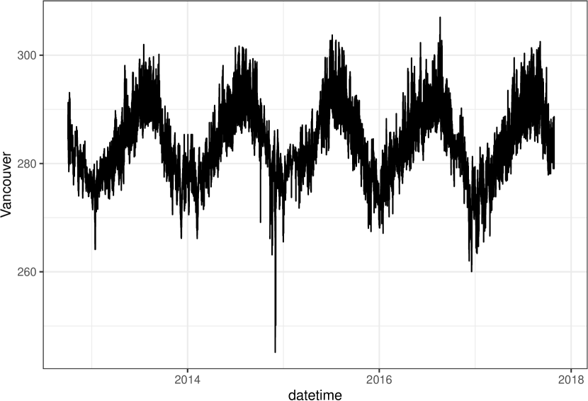
Figure 10: Plot for the Temperature dataset in Example 3.

# Load the hourly data consumption data

data <- data.table::fread("data/temperature.csv")

summary(data[, c("datetime", "Vancouver")])

##     datetime                     Vancouver
##  Min.   :2012-10-01 12:00:00   Min.   :245.2
##  1st Qu.:2014-01-15 21:00:00   1st Qu.:279.2
##  Median :2015-05-02 06:00:00   Median :283.4
##  Mean   :2015-05-02 06:00:00   Mean   :283.9
##  3rd Qu.:2016-08-15 15:00:00   3rd Qu.:288.6
##  Max.   :2017-11-30 00:00:00   Max.   :307.0
##                                NA’s   :795

# Load the cleanTS library

library(cleanTS)

# Use the `cleanTS()` function for cleaning the data.

cts <- cleanTS(data = data, date_format = "ymdHMs",

    time = "datetime", value = "Vancouver")

# The dataset contains multiples columns, so the time and

# value argument is used to specify the `timestamp` and to

# specify the `timestamp` and `observation` columns manually.

# The `cleanTS()` function returns a cleanTS object.

summary(cts)

##                  Length Class      Mode
## clean_data       5      data.table list
## missing_ts       0      POSIXct    numeric
## duplicate_ts     0      POSIXct    numeric
## imp_methods      4      -none-     character
## mcar_err         4      data.frame list
## mar_err          4      data.frame list
## outliers         4      data.table list
## outlier_mcar_err 4      data.frame list
## outlier_mar_err  4      data.frame list

# Print the cleanTS object

print(cts)

## $clean_data
## # A tibble: 45,253 x 5
##    time                value missing_type method_used      is_outlier
##    <dttm>              <dbl> <chr>        <chr>            <lgl>
##  1 2012-10-01 12:00:00  285. mcar         na_interpolation FALSE
##  2 2012-10-01 13:00:00  285. <NA>         <NA>             FALSE
##  3 2012-10-01 14:00:00  285. <NA>         <NA>             FALSE
##  4 2012-10-01 15:00:00  285. <NA>         <NA>             FALSE
##  5 2012-10-01 16:00:00  285. <NA>         <NA>             FALSE
##  6 2012-10-01 17:00:00  285. <NA>         <NA>             FALSE
##  7 2012-10-01 18:00:00  285. <NA>         <NA>             FALSE
##  8 2012-10-01 19:00:00  285. <NA>         <NA>             FALSE
##  9 2012-10-01 20:00:00  285. <NA>         <NA>             FALSE
## 10 2012-10-01 21:00:00  285. <NA>         <NA>             FALSE
## # ... with 45,243 more rows
##
## $missing_ts
## POSIXct of length 0
##
## $duplicate_ts
## POSIXct of length 0
##
## $imp_methods
## [1] "na_interpolation, na_locf, na_ma, na_kalman"
##
## $mcar_err
## # A tibble: 1 x 4
##   na_interpolation na_locf   na_ma na_kalman
##              <dbl>   <dbl>   <dbl>     <dbl>
## 1          0.00160 0.00258 0.00213   0.00164
##
## $mar_err
## # A tibble: 1 x 4
##   na_interpolation na_locf na_ma na_kalman
##              <dbl>   <dbl> <dbl>     <dbl>
## 1            0.493   0.584 0.571      3.09
##
## $outliers
## # A tibble: 33 x 4
##    time                value orig_value method_used
##    <dttm>              <dbl>      <dbl> <chr>
##  1 2014-10-05 18:00:00  290.       269. na_ma
##  2 2014-11-10 18:00:00  279.       266. na_kalman
##  3 2014-11-10 19:00:00  281.       267. na_kalman
##  4 2014-11-10 20:00:00  282.       270. na_kalman
##  5 2014-11-18 19:00:00  271.       263. na_kalman
##  6 2014-11-18 20:00:00  271.       267. na_kalman
##  7 2014-11-20 08:00:00  275.       265. na_ma
##  8 2014-11-29 22:00:00  271.       271. na_kalman
##  9 2014-11-29 23:00:00  270.       271. na_kalman
## 10 2014-11-30 00:00:00  270.       270. na_kalman
## # ... with 23 more rows
##
## $outlier_mcar_err
## # A tibble: 1 x 4
##   na_interpolation na_locf   na_ma na_kalman
##              <dbl>   <dbl>   <dbl>     <dbl>
## 1          0.00697  0.0122 0.00648   0.00704
##
## $outlier_mar_err
## # A tibble: 1 x 4
##   na_interpolation na_locf  na_ma na_kalman
##              <dbl>   <dbl>  <dbl>     <dbl>
## 1           0.0659  0.0974 0.0708    0.0471

# Use the `gen.report()` function to get a detailed report.

gen.report(cts)

##
## # Summary of cleaned data:
##    Min. 1st Qu.  Median    Mean 3rd Qu.    Max.
##   260.1   279.2   283.6   283.9   288.5   305.4
##
## # Missing timestamps:  0
##
## No missing timestamps found.
##
## # Duplicate timestamps:  0
##
## No duplicate timestamps found.
##
## # Missing Values:  795 (1.75678960510905%)
##
## ## MCAR:  1 (0.00220979824542019%)
##  MCAR Errors:
##   na_interpolation     na_locf       na_ma   na_kalman
## 1      0.001603655 0.002577279 0.002134501 0.001635805
##
##                   time  value      method_used
## 1: 2012-10-01 12:00:00 284.63 na_interpolation
##
##
## ## MAR:  794 (1.75457980686363%)
##  MAR Errors:
##   na_interpolation  na_locf     na_ma na_kalman
## 1        0.4931633 0.583915 0.5714428  3.094038
##                     time    value      method_used
##   1: 2013-03-11 07:00:00 278.6433 na_interpolation
##   2: 2013-03-11 08:00:00 278.5267 na_interpolation
##   3: 2017-10-28 01:00:00 288.0100 na_interpolation
##   4: 2017-10-28 02:00:00 288.0100 na_interpolation
##   5: 2017-10-28 03:00:00 288.0100 na_interpolation
##  ---
## 790: 2017-11-29 20:00:00 288.0100 na_interpolation
## 791: 2017-11-29 21:00:00 288.0100 na_interpolation
## 792: 2017-11-29 22:00:00 288.0100 na_interpolation
## 793: 2017-11-29 23:00:00 288.0100 na_interpolation
## 794: 2017-11-30 00:00:00 288.0100 na_interpolation
##
## # Outliers:  33
##                    time    value orig_value method_used
##  1: 2014-10-05 18:00:00 289.7553   269.1500       na_ma
##  2: 2014-11-10 18:00:00 279.3756   266.1500   na_kalman
##  3: 2014-11-10 19:00:00 280.7293   267.1500   na_kalman
##  4: 2014-11-10 20:00:00 281.9608   269.7883   na_kalman
##  5: 2014-11-18 19:00:00 270.9114   263.1500   na_kalman
##  6: 2014-11-18 20:00:00 271.0321   266.6466   na_kalman
##  7: 2014-11-20 08:00:00 274.9799   264.8900       na_ma
##  8: 2014-11-29 22:00:00 270.5659   270.5791   na_kalman
##  9: 2014-11-29 23:00:00 270.4940   270.5400   na_kalman
## 10: 2014-11-30 00:00:00 270.3393   270.3260   na_kalman
## 11: 2014-11-30 01:00:00 270.1110   269.8300   na_kalman
## 12: 2014-11-30 02:00:00 269.8186   269.5400   na_kalman
## 13: 2014-11-30 08:00:00 268.1006   266.8008       na_ma
## 14: 2014-11-30 16:00:00 267.4040   266.3400   na_kalman
## 15: 2014-11-30 17:00:00 268.0969   266.3906   na_kalman
## 16: 2014-11-30 18:00:00 268.8950   258.7303   na_kalman
## 17: 2014-11-30 19:00:00 269.7435   245.1500   na_kalman
## 18: 2014-11-30 20:00:00 270.5876   248.9412   na_kalman
## 19: 2014-11-30 21:00:00 271.3725   254.9672   na_kalman
## 20: 2014-12-02 16:00:00 270.0522   266.9844       na_ma
## 21: 2014-12-02 18:00:00 271.7652   267.3107   na_kalman
## 22: 2014-12-02 19:00:00 273.3105   250.1500   na_kalman
## 23: 2016-06-06 00:00:00 301.6683   302.3100   na_kalman
## 24: 2016-06-06 01:00:00 301.3838   301.9200   na_kalman
## 25: 2016-06-06 02:00:00 300.8096   301.3100   na_kalman
## 26: 2016-08-19 21:00:00 305.1987   305.9000   na_kalman
## 27: 2016-08-19 22:00:00 305.3927   306.6900   na_kalman
## 28: 2016-08-19 23:00:00 305.2390   307.0000   na_kalman
## 29: 2016-08-20 00:00:00 304.7360   306.6900   na_kalman
## 30: 2016-08-20 01:00:00 303.8823   306.0600   na_kalman
## 31: 2016-08-20 02:00:00 302.6764   305.3000   na_kalman
## 32: 2016-12-18 03:00:00 265.3639   262.8000   na_kalman
## 33: 2016-12-18 04:00:00 263.9526   262.5300   na_kalman
##                    time    value orig_value method_used
## ## Imputation errors while replacing outliers:
## ### MCAR errors:
##   na_interpolation    na_locf       na_ma   na_kalman
## 1      0.006966497 0.01220904 0.006478862 0.007041101
## ### MAR errors:
##   na_interpolation    na_locf      na_ma  na_kalman
## 1       0.06589995 0.09743086 0.07080976 0.04711339

The output generated by the animate_interval() is a GIF, and therefore it is not possible to include it here. Similarly, the output of interactive_plot() is a interactive object cannot be shown. These outputs for all the examples shown here are available at this link: Link to Outputs (https://drive.google.com/drive/folders/1NYvHcib2JGDgPSyN_3uAYOBO6Dv8N6di?usp=sharing).

Current code version

Nr.	Code metadata description	Please fill in this column
C1	Current code version	v0.1.0
C2	Permanent link to code/repository used for this code version	$https://github.com/Mayur1009/cleanTS$, $https://cran.r-project.org/package=cleanTS$
C3	Permanent link to Reproducible Capsule
C4	Legal Code License	GNU General Public License v3.0
C5	Code versioning system used	git
C6	Software code languages, tools, and services used	R programming language
C7	Compilation requirements, operating environments & dependencies
C8	If available Link to developer documentation/manual	$https://mayur1009.github.io/cleanTS/$
C9	Support email for questions	$mayur.k.shende@gmail.com$, $neerajdhanraj@cae.au.dk$, $afeijoo@uvigo.gal$

Table 7: Code metadata (mandatory)

References

- [1] G. E. Box, G. M. Jenkins, G. C. Reinsel, G. M. Ljung, Time series analysis: forecasting and control, John Wiley & Sons, 2015.
- [2] P. J. Brockwell, R. A. Davis, Introduction to time series and forecasting (2016).
- [3] J. D. Hamilton, Time series analysis.
- [4] N. Bokde, A. Feijóo, D. Villanueva, K. Kulat, A review on hybrid empirical mode decomposition models for wind speed and wind power prediction, Energies 12 (2) (2019) 254.
- [5] A. Gupta, N. Bokde, K. Kulat, Hybrid leakage management for water network using psf algorithm and soft computing techniques, Water resources management 32 (3) (2018) 1133–1151.
- [6] Z. Bar-Joseph, G. K. Gerber, D. K. Gifford, T. S. Jaakkola, I. Simon, Continuous representations of time-series gene expression data, Journal of Computational Biology 10 (3-4) (2003) 341–356.
- [7] J. M. Gottman, Time-series analysisa comprehensive introduction for social scientists, no. 519.55 G6, 1981.
- [8] M. Ghil, R. Vautard, Interdecadal oscillations and the warming trend in global temperature time series, Nature 350 (6316) (1991) 324–327.
- [9] J. C. Cuaresma, J. Hlouskova, S. Kossmeier, M. Obersteiner, Forecasting electricity spot-prices using linear univariate time-series models, Applied Energy 77 (1) (2004) 87–106.
- [10] N. Bokde, B. Tranberg, G. B. Andresen, A graphical approach to carbon-efficient spot market scheduling for power-to-x applications, Energy Conversion and Management 224 (2020) 113461.
- [11] S. J. Taylor, Modelling financial time series, Tech. rep., World Scientific Publishing Co. Pte. Ltd. (2007).
- [12] R. Billinton, H. Chen, R. Ghajar, Time-series models for reliability evaluation of power systems including wind energy, Microelectronics Reliability 36 (9) (1996) 1253–1261.
- [13] N. Bokde, A. Troncoso, G. Asencio-Cortes, K. Kulat, F. Martinez-Alvarez, Pattern sequence similarity based techniques for wind speed forecasting, in: Proceedings of the International Work-Conference on Time Series, Granada, Spain, 2017, pp. 18–20.
- [14] N. Bokde, A. Feijoo, N. Al-Ansari, S. Tao, Z. M. Yaseen, The hybridization of ensemble empirical mode decomposition with forecasting models: Application of short-term wind speed and power modeling, Energies 13 (7) (2020) 1666.
- [15] A. Chatterjee, M. W. Gerdes, S. G. Martinez, Statistical explorations and univariate timeseries analysis on covid-19 datasets to understand the trend of disease spreading and death, Sensors 20 (11) (2020) 3089.
- [16] X. Wang, C. Wang, Time series data cleaning: A survey, IEEE Access 8 (2019) 1866–1881.
- [17] H. Wickham, G. Grolemund, R for Data Science: Import, Tidy, Transform, Visualize, and Model Data, 1st Edition, O’Reilly Media, Inc., 2017.
- [18] H. Chen, R. H. Chiang, V. C. Storey, Business intelligence and analytics: From big data to big impact, MIS quarterly (2012) 1165–1188.
- [19] T. H. Davenport, J. G. Harris, et al., Competing on Analytics: The New Science of Winning, Harvard Business Press, 2007.
- [20] E.-P. Lim, H. Chen, G. Chen, Business intelligence and analytics: Research directions, ACM Transactions on Management Information Systems (TMIS) 3 (4) (2013) 1–10.
- [21] S. Chaudhuri, U. Dayal, V. Narasayya, An overview of business intelligence technology, Communications of the ACM 54 (8) (2011) 88–98.
- [22] H. J. Watson, B. H. Wixom, The current state of business intelligence, Computer 40 (9) (2007) 96–99.
- [23] K. Ayankoya, A. Calitz, J. Greyling, Intrinsic relations between data science, big data, business analytics and datafication, in: Proceedings of the Southern African Institute for Computer Scientist and Information Technologists Annual Conference 2014 on SAICSIT 2014 Empowered by Technology, 2014, pp. 192–198.
- [24] A. T. Lo’ai, R. Mehmood, E. Benkhlifa, H. Song, Mobile cloud computing model and big data analysis for healthcare applications, IEEE Access 4 (2016) 6171–6180.
- [25] H. C. Koh, G. Tan, et al., Data mining applications in healthcare, Journal of healthcare information management 19 (2) (2011) 65.
- [26] A. A. Cardenas, P. K. Manadhata, S. P. Rajan, Big data analytics for security, IEEE Security & Privacy 11 (6) (2013) 74–76.
- [27] S. R. Jeffery, G. Alonso, M. J. Franklin, W. Hong, J. Widom, Declarative support for sensor data cleaning, in: International Conference on Pervasive Computing, Springer, 2006, pp. 83–100.
- [28] F. Mörchen, Time series knowledge mining, Citeseer, 2006.
- [29] A. Zhang, S. Song, J. Wang, P. S. Yu, Time series data cleaning: From anomaly detection to anomaly repairing, Proceedings of the VLDB Endowment 10 (10) (2017) 1046–1057.
- [30] Z. Xing, J. Pei, S. Y. Philip, Early classification on time series, Knowledge and information systems 31 (1) (2012) 105–127.
-
[31]
M. Shende, N. Bokde, A. E. Feijóo-Lorenzo,
cleanTS: Testbench for
Univariate Time Series Cleaning, r package version 0.1.0 (2021).
URL https://CRAN.R-project.org/package=cleanTS - [32] A. Karkouch, H. Mousannif, H. Al Moatassime, T. Noel, Data quality in internet of things: A state-of-the-art survey, Journal of Network and Computer Applications 73 (2016) 57–81.
- [33] F. N. Afrati, P. G. Kolaitis, Repair checking in inconsistent databases: algorithms and complexity, in: Proceedings of the 12th International Conference on Database Theory, 2009, pp. 31–41.
- [34] J. Chomicki, J. Marcinkowski, Minimal-change integrity maintenance using tuple deletions, Information and Computation 197 (1-2) (2005) 90–121.
- [35] R. Fagin, B. Kimelfeld, P. G. Kolaitis, Dichotomies in the complexity of preferred repairs, in: Proceedings of the 34th ACM SIGMOD-SIGACT-SIGAI Symposium on Principles of Database Systems, 2015, pp. 3–15.
- [36] X. Ding, H. Wang, J. Su, Z. Li, J. Li, H. Gao, Cleanits: A data cleaning system for industrial time series, Proceedings of the VLDB Endowment 12 (12) (2019) 1786–1789.
- [37] J. Wang, H. Zhang, B. Fang, X. Wang, G. Yin, X. Yu, Edcleaner: Data cleaning for entity information in social network, in: ICC 2019-2019 IEEE International Conference on Communications (ICC), IEEE, 2019, pp. 1–7.
- [38] R. Huang, Z. Chen, Z. Liu, S. Song, J. Wang, Tsoutlier: Explaining outliers with uniform profiles over iot data, in: 2019 IEEE International Conference on Big Data (Big Data), IEEE, 2019, pp. 2024–2027.
- [39] K. Rong, P. Bailis, Asap: prioritizing attention via time series smoothing, arXiv preprint arXiv:1703.00983 (2017).
- [40] Y. Huang, M. Milani, F. Chiang, Pacas: privacy-aware, data cleaning-as-a-service, in: 2018 IEEE International Conference on Big Data (Big Data), IEEE, 2018, pp. 1023–1030.
- [41] Z. Yu, X. Chu, Piclean: A probabilistic and interactive data cleaning system, in: Proceedings of the 2019 International Conference on Management of Data, 2019, pp. 2021–2024.
- [42] T. Rekatsinas, X. Chu, I. F. Ilyas, C. Ré, Holoclean: Holistic data repairs with probabilistic inference, arXiv preprint arXiv:1702.00820 (2017).
- [43] S. Krishnan, J. Wang, E. Wu, M. J. Franklin, K. Goldberg, Activeclean: Interactive data cleaning for statistical modeling, Proceedings of the VLDB Endowment 9 (12) (2016) 948–959.
- [44] K. H. Tae, Y. Roh, Y. H. Oh, H. Kim, S. E. Whang, Data cleaning for accurate, fair, and robust models: A big data-ai integration approach, in: Proceedings of the 3rd International Workshop on Data Management for End-to-End Machine Learning, 2019, pp. 1–4.
- [45] S. Moritz, A. Sardá, T. Bartz-Beielstein, M. Zaefferer, J. Stork, Comparison of different methods for univariate time series imputation in r, arXiv preprint arXiv:1510.03924 (2015).
- [46] D. J. Stekhoven, P. Bühlmann, Missforest—non-parametric missing value imputation for mixed-type data, Bioinformatics 28 (1) (2012) 112–118.
- [47] N. L. Crookston, A. O. Finley, yaimpute: an r package for knn imputation, Journal of Statistical Software. 23 (10). 16 p. (2008).
- [48] F. Meinfelder, Package’baboon’: Bayesian bootstrap predictive mean matching-multiple and single imputation for discrete data; version 0.1-6.
- [49] K. Gross, D. Bates, mvnmle: Ml estimation for multivariate normal data with missing values. r package version 0.1–10 (2011).
- [50] F. M. L. Di Lascio, S. Giannerini, A. Reale, Imputation of complex dependent data by conditional copulas: analytic versus semiparametric approach, in: Book of proceedings of the 21st International Conference on Computational Statistics (COMPSTAT 2014), Citeseer, 2014, pp. 491–497.
-
[51]
W. Junger, A. P. de Leon,
mtsdi: Multivariate Time
Series Data Imputation, r package version 0.3.5 (2018).
URL https://CRAN.R-project.org/package=mtsdi - [52] S. Moritz, T. Bartz-Beielstein, imputets: time series missing value imputation in r., R J. 9 (1) (2017) 207.
- [53] A. Kowarik, M. Templ, Imputation with the R package VIM, Journal of Statistical Software 74 (7) (2016) 1–16. doi:10.18637/jss.v074.i07.
- [54] N. Laptev, S. Amizadeh, I. Flint, Generic and scalable framework for automated time-series anomaly detection, in: Proceedings of the 21th ACM SIGKDD international conference on knowledge discovery and data mining, 2015, pp. 1939–1947.
- [55] C. C. Aggarwal, Outlier analysis, in: Data mining, Springer, 2015, pp. 237–263.
-
[56]
R Core Team, R: A Language and Environment
for Statistical Computing, R Foundation for Statistical Computing, Vienna,
Austria (2021).
URL https://www.R-project.org/ -
[57]
M. Dowle, A. Srinivasan,
data.table: Extension of
‘data.frame‘, r package version 1.14.0 (2021).
URL https://CRAN.R-project.org/package=data.table - [58] H. Wickham, M. Averick, J. Bryan, W. Chang, L. D. McGowan, R. François, G. Grolemund, A. Hayes, L. Henry, J. Hester, M. Kuhn, T. L. Pedersen, E. Miller, S. M. Bache, K. Müller, J. Ooms, D. Robinson, D. P. Seidel, V. Spinu, K. Takahashi, D. Vaughan, C. Wilke, K. Woo, H. Yutani, Welcome to the tidyverse, Journal of Open Source Software 4 (43) (2019) 1686. doi:10.21105/joss.01686.
-
[59]
H. Wickham, R. François, L. Henry, K. Müller,
dplyr: A Grammar of Data
Manipulation, r package version 1.0.5 (2021).
URL https://CRAN.R-project.org/package=dplyr -
[60]
K. Müller, H. Wickham,
tibble: Simple Data Frames,
r package version 3.1.1 (2021).
URL https://CRAN.R-project.org/package=tibble -
[61]
H. Wickham, ggplot2: Elegant Graphics for
Data Analysis, Springer-Verlag New York, 2016.
URL https://ggplot2.tidyverse.org -
[62]
H. Wickham, tidyr: Tidy Messy
Data, r package version 1.1.3 (2021).
URL https://CRAN.R-project.org/package=tidyr -
[63]
data.table vs dplyr (2020).
URL https://stackoverflow.com/q/21435339 -
[64]
G. Grolemund, H. Wickham, Dates and
times made easy with lubridate, Journal of Statistical Software 40 (3)
(2011) 1–25.
URL https://www.jstatsoft.org/v40/i03/ -
[65]
lubridate
(2020).
URL https://lubridate.tidyverse.org/reference/parse_date_time.html - [66] M. W. Beck, N. Bokde, G. Ascencio-Cort’es, K. Kulat, R package imputeTestbench to Compare Imputation Methods for Univarite Time Series, The R Journal 10 (1) (2018) 218–233. doi:10.32614/RJ-2018-024.
- [67] N. Bokde, K. Kulat, M. W. Beck, G. Asencio-Cortés, R package imputetestbench to compare imputations methods for univariate time series, arXiv preprint arXiv:1608.00476 (2016).
- [68] S. Moritz, T. Bartz-Beielstein, imputeTS: Time Series Missing Value Imputation in R, The R Journal 9 (1) (2017) 207–218. doi:10.32614/RJ-2017-009.
-
[69]
M. Dancho, D. Vaughan,
anomalize: Tidy Anomaly
Detection, r package version 0.2.2 (2020).
URL https://CRAN.R-project.org/package=anomalize -
[70]
D. Vaughan, M. Dancho,
tibbletime: Time Aware
Tibbles, r package version 0.1.6 (2020).
URL https://CRAN.R-project.org/package=tibbletime -
[71]
T. L. Pedersen, D. Robinson,
gganimate: A Grammar of
Animated Graphics, r package version 1.0.7 (2020).
URL https://CRAN.R-project.org/package=gganimate -
[72]
W. Chang, J. Cheng, J. Allaire, C. Sievert, B. Schloerke, Y. Xie, J. Allen,
J. McPherson, A. Dipert, B. Borges,
shiny: Web Application
Framework for R, r package version 1.6.0 (2021).
URL https://CRAN.R-project.org/package=shiny -
[73]
O. Mersmann,
microbenchmark:
Accurate Timing Functions, r package version 1.4-7 (2019).
URL https://CRAN.R-project.org/package=microbenchmark -
[74]
Power
Comsumption (2018).
URL https://www.kaggle.com/robikscube/hourly-energy-consumption - [75] N. D. Bokde, B. Tranberg, G. B. Andresen, Short-term co2 emissions forecasting based on decomposition approaches and its impact on electricity market scheduling, Applied Energy 281 116061.
- [76] N. D. Bokde, T. T. Pedersen, G. B. Andresen, Optimal scheduling of flexible power-to-x technologies in the day-ahead electricity market (2021). arXiv:2110.09800.
-
[77]
Historical
Hourly Weather Data 2012-2017 (2017).
URL https://www.kaggle.com/selfishgene/historical-hourly-weather-data