Testing network correlation efficiently via counting trees

Abstract

We propose a new procedure for testing whether two networks are edge-correlated through some latent vertex correspondence. The test statistic is based on counting the co-occurrences of signed trees for a family of non-isomorphic trees. When the two networks are Erdős–Rényi random graphs ${\mathcal{G}}(n,q)$ that are either independent or correlated with correlation coefficient $\rho$, our test runs in $n^{2+o(1)}$ time and succeeds with high probability as $n\to\infty$, provided that $n\min\{q,1-q\}\geq n^{-o(1)}$ and $\rho^{2}>\alpha\approx 0.338$, where $\alpha$ is Otter’s constant so that the number of unlabeled trees with $K$ edges grows as $(1/\alpha)^{K}$. This significantly improves the prior work in terms of statistical accuracy, running time, and graph sparsity.

1 Introduction

In recent years, there is a surge of interest in studying the problem of graph matching or network alignment, which aims to find the latent vertex correspondence between the two graphs solely based on their network topologies. This paradigm arises in a suite of diverse applications, such as social network analysis [NS08, NS09], computer vision [CSS07, BBM05], computational biology [CSS07, BBM05], and natural language processing [HNM05, BGSW13].

Finding the optimal vertex correspondence that best aligns the two graphs amounts to solving the the NP-hard quadratic assignment problem (QAP). Aiming to circumvent its worst-case intractability, a popular statistical model for graph matching is the correlated Erdős–Rényi graph model, denoted by ${\mathcal{G}}(n,q,\rho)$, in which the observed graphs are two instances of the Erdős–Rényi graph ${\mathcal{G}}(n,q)$ whose edges are correlated through a hidden vertex correspondence. Specifically, let $\pi$ be a latent uniform random permutation on $[n]\triangleq\{1,\ldots,n\}$. Denote the observed graphs by $G_{1}$ and $G_{2}$ and their adjacency matrices by $A=(A_{ij})$ and $B=(B_{ij})$ respectively. Conditioned on the permutation $\pi$, the pairs of edges $\{(A_{ij},B_{\pi(i)\pi(j)}):1\leq i<j\leq n\}$ are i.i.d. pairs of Bernoulli random variables with parameter $q\in(0,1)$ and correlation coefficient $\rho$. In the special case of $\rho>0$, $A$ and $B^{\pi}=(B_{\pi(i)\pi(j)})$ can be viewed as adjacency matrices of two children graphs that are independently edge-subsampled from a common parent Erdős–Rényi graph ${\mathcal{G}}(n,p)$ with subsampling probability $s$, where $p=q/s$ and $s=\rho(1-q)+q$ [PG11]. The goal is to recover the true vertex mapping $\pi$ based on $G_{1}$ and $G_{2}$. Under the correlated Erdős–Rényi graph model, the information-theoretic thresholds for both exact and partial recovery have been characterized [CK16, CK17, HM20, WXY21] and various efficient matching algorithms with provable performance guarantees have been devised [FQRM⁺16, LFF⁺16, DMWX18, BCL⁺19, FMWX19a, FMWX19b, GM20, GML21, MRT21b, MRT21a].

1.1 Detecting network correlation

Despite the significant amount of research activities and remarkable progress in the graph matching problem, relatively less attention has been paid to the even more basic problem of detecting the presence of correlation in network topology between two otherwise independently generated graphs. This problem is practically important in many aforementioned application domains such as detecting similar $3$-D objects in computer vision or similar biological networks across different species. From a theoretical point of view, network correlation detection can be viewed as a natural extension of the classical problem of correlation detection for vector data (testing the correlation between two random vectors under an unknown orthogonal transformation [Ste79]) to network data. In addition, the detection problem offers insights into the computational limits of graph matching; see Section 2.3 for an in-depth discussion.

Following [BCL⁺19, WXY20], we formulate the problem of detecting network correlation as a hypothesis testing problem, where

• Under the null hypothesis ${\mathcal{H}}_{0}$, $G_{1}$ and $G_{2}$ are independently generated from the Erdős–Rényi graph model ${\mathcal{G}}(n,q)$;

• Under the alternative hypothesis, ${\mathcal{H}}_{1}$, $G_{1}$ and $G_{2}$ are generated from the correlated Erdős–Rényi graph model ${\mathcal{G}}(n,q,\rho)$.

Note that under both ${\mathcal{H}}_{0}$ and ${\mathcal{H}}_{1}$, the graphs $G_{1}$ and $G_{2}$ are marginally distributed as ${\mathcal{G}}(n,q)$. The goal is to distinguish ${\mathcal{H}}_{0}$ from ${\mathcal{H}}_{1}$ based on the observation of $G_{1}$ and $G_{2}$. We say a test statistic $f(G_{1},G_{2})$ with threshold $\tau\in{\mathbb{R}}$ achieves consistent detection if the sum of type I and type II errors converges to 0 as $n\to\infty$, that is,

$$\lim_{n\to\infty}\left[{\mathcal{Q}}(f(G_{1},G_{2})\geq\tau)+{\mathcal{P}}(f(G_{1},G_{2})<\tau)\right]=0,$$ (1)

where ${\mathcal{Q}}$ and ${\mathcal{P}}$ denote the joint distribution of $G_{1}$ and $G_{2}$ under ${\mathcal{H}}_{0}$ and ${\mathcal{H}}_{1}$, respectively.

1.2 Subgraph counts

Note that due to the latent random vertex mapping $\pi$, the problem is equivalent to testing the correlation between two unlabeled graphs. Thus, any test must rely on on graph invariants — graph properties that are invariant under graph isomorphisms, such as subgraph counts or graph eigenvalues. This paper adopts a strategy based on subgraph counts and improves upon prior works [BCL⁺19, WXY20], which we now discuss.

In order to determine the information-theoretic limit, [WXY20] considered the QAP test statistic, namely, the maximum number of common edges between $G_{1}$ and $G_{2}$ over all possible vertex correspondences, which by definition is invariant under isomorphisms of both graphs (Equivalently, this test can be viewed as finding the maximum common subgraph of $G_{1}$ and $G_{2}$). The QAP test is shown to achieve the optimal detection threshold with sharp constant in the dense regime and within constant factors in the sparse regime. The drawback of this test is the computational intractability of solving the QAP. In addition, a simple test based on comparing the number of edges in $G_{1}$ and $G_{2}$ is also analyzed in [WXY20]; however, its statistical power is weak, requiring the correlation parameter $\rho$ to approach $1$ to achieve consistent detection.

To obtain a more powerful yet computationally efficient statistic, a natural idea is to count more complex subgraphs than edges. Specifically, let $\mathsf{sub}(H,G)$ denote the subgraph count, i.e., the number of copies, of $H$ in $G$. Crucially, for any given graph $H$, $\mathsf{sub}(H,G_{1})$ and $\mathsf{sub}(H,G_{2})$ are independent under ${\mathcal{H}}_{0}$ but correlated under ${\mathcal{H}}_{1}$. Thus, one can distinguish ${\mathcal{H}}_{0}$ and ${\mathcal{H}}_{1}$ by thresholding on the covariance of $\mathsf{sub}(H,G_{1})$ and $\mathsf{sub}(H,G_{2})$, that is,

$$P_{H}\triangleq\left(\mathsf{sub}(H,G_{1})-\mathbb{E}\left[\mathsf{sub}(H,G_{1})\right]\right)\left(\mathsf{sub}(H,G_{2})-\mathbb{E}\left[\mathsf{sub}(H,G_{2})\right]\right)\,.$$

However, counting a single graph $H$ may not suffice, especially when the graphs are sparse and the correlation is weak. To obtain a better test statistic, [BCL⁺19] considers a large family ${\mathcal{H}}$ of non-isomorphic subgraphs and further sum $P_{H}$ over $H\in{\mathcal{H}}$. A key step in the analysis is to ensure that $P_{H}$’s are approximately independent across different $H$ so that the $\sum_{H\in{\mathcal{H}}}P_{H}$ has a relatively small variance; this requires a careful choice of the collection ${\mathcal{H}}$.

To this end, [BCL⁺19] proposes to count a family of the so-called (strictly) balanced graphs. A graph $H$ is called (strictly) balanced if every proper subgraph of $H$ is (strictly) less dense than the graph $H$ itself, where the density is defined as the number of edges divided by the number of nodes. It is well known in random graph theory that strict balancedness ensures that the subgraph counts are well concentrated [JLR11, Chapter 3]. Specifically, [BCL⁺19] gives a probabilistic construction of a family ${\mathcal{H}}$ of strictly balanced graphs of a constant size $K$ and a constant edge density $\eta>1$, assuming $nq^{\eta}=\Theta(1)$. Under this choice, it is shown that the test statistic $\sum_{H\in{\mathcal{H}}}P_{H}$ distinguishes between the two hypotheses with probability at least $0.9$, when $\rho=\Omega(1)$ and the average degree $nq$ belongs to $[n^{\epsilon},n^{1/153}]\cup[n^{2/3},n^{1-\epsilon}]$ for any small constant $\epsilon>0$.

While the test in [BCL⁺19] succeeds under small correlation $\rho$, it still has several key limitations. First, the existing performance guarantee in [BCL⁺19] requires the average degree $nq$ to fall into a very specific range and in particular does not accommodate sparse graphs such as $nq=O(1)$; this restriction originates from the construction of strictly balanced graphs based on random regular graphs. Second, as an exhaustive search of subgraphs of size $K$ takes $n^{O(K)}$ time, in order to achieve a polynomial run time, [BCL⁺19] only counts subgraphs of constant size $K=\Theta(1)$, which precludes the possibility of achieving a vanishing error probability. Third, to tolerate small correlation $\rho$, $K$ needs to be as large as $(1/\rho)^{C}$ for a large constant $C$, leading to a time complexity of $n^{(1/\rho)^{C}}$, which can be prohibitive for large networks.

In this paper, we propose a new test that runs in time $n^{2+o(1)}$ and succeeds with high probability as long as $\rho^{2}$ exceeds $0.338$ and $n\min\{q,1-q\}\geq n^{-o(1)}$, i.e., the graphs are not overly sparse or dense. This significantly improves on the previous results in [BCL⁺19, WXY20] in terms of graph sparsity, testing error, and computational complexity.

Our main strategy is to count trees of $K$ edges in the observed graphs, where, crucially, $K$ grows with $n$. While by definition a tree with $K$ edges is also strictly balanced with density $K/(K+1)$, our test statistic is fundamentally different from that in [BCL⁺19]. In particular, if we adopt their test statistic with ${\mathcal{H}}$ being the collection of trees with $K$ edges, their existing result requires $nq^{K/(K+1)}=\Theta(1)$ and thus cannot deal with the most interesting case of $nq\geq 1$. In fact, when $nq\geq 1$, for any two non-isomorphic trees $H\not\cong H^{\prime}$, the covariance between $\mathsf{sub}(H,G_{1})$ and $\mathsf{sub}(H^{\prime},G_{1})$ is on the same order as the variance of $\mathsf{sub}(H,G_{1})$. As a consequence, the covariance between $P_{H}$ and $P_{H^{\prime}}$ is relatively large compared to $(\mathbb{E}\left[P_{H}\right])^{2}$ under ${\mathcal{H}}_{1}$. Hence, the standard deviation of $\sum_{H\in{\mathcal{H}}}P_{H}$ is on par with its mean under ${\mathcal{H}}_{1}$, leading to the likely failure of the test statistic in [BCL⁺19]. Therefore, a key challenge is how to better utilize the tree counts so that the correlation between the counts of non-isomorphic trees does not overwhelm the signal — the correlation of counts of isomorphic trees.

Furthermore, direct enumeration of trees of size $K$ takes $n^{O(K)}$ time which is super-polynomial if $K$ grows with $n$. To resolve this issue, we leverage the idea of color coding [AYZ95, AR02, HS17] to develop an $n^{2}e^{O(K)}$-time algorithm that approximates our test statistic and succeeds under the same condition. When applied to the correlated Erdős–Rényi model, $K$ can be chosen to grow with $n$ arbitrarily slowly so that the test runs in $n^{2+o(1)}$ time.

1.3 Notation and paper organization

For any graph $H$, let $V(H)$ denote the vertex set of $H$ and $E(H)$ denote the edge set of $H$. Two graphs $H$ and $H^{\prime}$ are isomorphic, denoted by $H\cong H^{\prime}$, if there exists a bijection $\pi:V(H)\to V(H^{\prime})$ such that $(\pi(u),\pi(v))\in E(H^{\prime})$ if and only if $(u,v)\in E(H)$. Denote by $[H]$ the isomorphism class of $H$; it is customary to refer to these isomorphic classes as unlabeled graphs. Let $\mathsf{aut}(H)$ be the number of automorphisms of $H$ (graph isomorphisms to itself). We say $H$ is a subgraph of $G$, denoted by $H\subset G$, if $V(H)\subset V(G)$ and $E(H)\subset E(G)$. We define $\mathsf{sub}(H,G)$ as the number of subgraphs in $G$ that are isomorphic to $H$, i.e., $\mathsf{sub}(H,G)\triangleq\sum_{H^{\prime}\subset G}{\mathbf{1}_{\left\{{H^{\prime}\cong H}\right\}}}$. For example, $\mathsf{sub}(\leavevmode\hbox to17.63pt{\vbox to3.4pt{\text{[drawing]}}},\;\leavevmode\hbox to10.51pt{\vbox to10.51pt{\text{[drawing]}}})=8$. Denoting by $K_{n}$ the complete graph with vertex set $[n]$ and edge set $\binom{[n]}{2}\triangleq\{\{u,v\}:u,v\in[n],\,u\neq v\}$, we abbreviate

$$\mathsf{sub}_{n}(H)\triangleq\mathsf{sub}(H,K_{n})=\binom{n}{|V(H)|}\frac{|V(H)|!}{\mathsf{aut}(H)},$$ (2)

where the equality follows by enumerating all possible vertex relabeling of $H$: $V(H)\to[n]$ modulo the automorphism of $H$ (see, e.g. [FK16, Lemma 5.1]). For each subset $S\subset\binom{[n]}{2}$, we identify it with an (edge-induced) subgraph of $K_{n}$. Let ${\mathcal{S}}_{n}$ denote the set of permutations $\pi:[n]\to[n]$. For a given permutation $\pi\in{\mathcal{S}}_{n}$, let $\pi(S)=\{(\pi(u),\pi(v)):(u,v)\in S\}$, which is identified with a relabeled version of $S$.

For two real numbers $a$ and $b$, we let $a\vee b\triangleq\max\{a,b\}$ and $a\wedge b\triangleq\min\{a,b\}$. We use standard asymptotic notation: For two sequences $\{a_{n}\}$ and $\{b_{n}\}$ of positive numbers, we write $a_{n}=O(b_{n})$, if $a_{n}\leq Cb_{n}$ for an absolute constant $C$ and for all $n$; $a_{n}=\Omega(b_{n})$, if $b_{n}=O(a_{n})$; $a_{n}=\Theta(b_{n})$, if $a_{n}=O(b_{n})$ and $a_{n}=\Omega(b_{n})$; $a_{n}=o(b_{n})$ or $b_{n}=\omega(a_{n})$, if $a_{n}/b_{n}\to 0$ as $n\to\infty$.

The rest of the paper is organized as follows. In Section 2, we first present the theoretical guarantees of our signed tree-counting statistic; then discuss the connection to the low-degree approximation of likelihood ratio and the computational hardness based on the low-degree approximation; and finally conclude this section with further related works. Section 3 provides the statistical analysis of our signed tree-counting statistic, with detailed proofs deferred to Appendix B. In Section 4.1, we present an efficient algorithm to approximately compute our signed tree-counting statistic based on color coding. Detailed proofs of the statistical and computational guarantees of the algorithm are postponed to Appendix C. In Section 5, we conduct numerical experiments to corroborate our theoretical findings. In addition, several preliminary facts on graphs are collected in Appendix A.

2 Main results and discussions

2.1 Test statistics and theoretical guarantees

Deviating from the previous approach of counting subgraphs in $G_{1}$ and $G_{2}$ directly [BCL⁺19], we propose to count trees in the centered version of $G_{1}$ and $G_{2}$, which we call signed trees following [BDER16]. Specifically, denote by $A$ and $B$ the adjacency matrices of $G_{1}$ and $G_{2}$ respectively, and by $\overline{A}=A-\mathbb{E}\left[A\right]$ and $\overline{B}=B-\mathbb{E}\left[B\right]$ their centered version. Let ${\mathcal{T}}$ denote the set of unlabeled trees with $K$ edges. For example, for $K=4$, ${\mathcal{T}}$ consists of three trees shown in pictograms below (see [HP59, App. I] for bigger examples)

$${\mathcal{T}}=\left\{\leavevmode\hbox to46.08pt{\vbox to3.4pt{\text{[drawing]}}}\,,\quad\leavevmode\hbox to24.74pt{\vbox to24.74pt{\text{[drawing]}}}\,,\quad\leavevmode\hbox to24.74pt{\vbox to24.74pt{\text{[drawing]}}}\right\}$$

and our test statistic is determined by the number of their copies in the observed graphs.

Define

$$f_{{\mathcal{T}}}(A,B)\triangleq\sum_{[H]\in{\mathcal{T}}}f_{H}(A,B),\quad\text{ where }f_{H}(A,B)\triangleq\beta\,\mathsf{aut}(H)W_{H}(\bar{A})W_{H}(\bar{B})\,.$$ (3)

Here

$$\beta=\left(\frac{\rho}{q(1-q)}\right)^{K}\frac{(n-K-1)!}{n!}$$ (4)

is a scaling factor introduced for ease of analysis, each $[H]\in{\mathcal{T}}$ is an unlabeled tree, and for any weighted adjacency matrix $M$ on vertex set $[n]$, we define

$$W_{H}(M)\triangleq\sum_{S\cong H}\prod_{(i,j)\in S}M_{ij}\,,$$ (5)

where the sum is over subgraphs of $K_{n}$ that are isomorphic to $H$. When $M$ is the unweighted adjacency matrix of a graph $G$, $W_{H}(M)$ reduces to the subgraph count $\mathsf{sub}(H,G)$. Thus $W_{H}(M)$ can be viewed as a natural generalization of the subgraph count to weighted graphs. Crucially, after centering $\mathbb{E}\left[W_{H}(\overline{A})W_{H^{\prime}}(\overline{A})\right]\neq 0$ if and only if $H\cong H^{\prime}$; the same identity holds for $\overline{B}$. This orthogonality property immediately implies that $f_{H}(A,B)$ and $f_{H^{\prime}}(A,B)$ are uncorrelated under the null hypothesis ${\mathcal{H}}_{0}$ for $H\ncong H^{\prime}$ and further enables us to control the correlation between $f_{H}(A,B)$ and $f_{H^{\prime}}(A,B)$ under ${\mathcal{H}}_{1}$. Indeed, we can readily show that $\mathbb{E}_{{\mathcal{Q}}}[f_{{\mathcal{T}}}(A,B)]=0$ and

$$\frac{(\mathbb{E}_{{\mathcal{P}}}[f_{{\mathcal{T}}}(A,B)])^{2}}{\mathrm{Var}_{\mathcal{Q}}[f_{{\mathcal{T}}}(A,B)]}=\rho^{2K}|{\mathcal{T}}|\,.$$

A celebrated result of Otter [Ott48] is that the number of unlabeled trees grows exponentially with

$$\lim_{K\to\infty}|{\mathcal{T}}|^{1/K}=1/\alpha,$$ (6)

where $\alpha\approx 0.33833$ is Otter’s constant. Therefore whenever the correlation satisfies $\rho^{2}>\alpha$, we have $\mathrm{Var}_{\mathcal{Q}}[f_{{\mathcal{T}}}]=o((\mathbb{E}_{{\mathcal{P}}}[f_{{\mathcal{T}}}])^{2})$. Furthermore, with additional assumptions, we can show that $\mathrm{Var}_{\mathcal{P}}[f_{{\mathcal{T}}}]=o((\mathbb{E}_{{\mathcal{P}}}[f_{{\mathcal{T}}}])^{2})$. This requires a delicate analysis of the covariance between $W_{H}(\overline{A})W_{H}(\overline{B})$ and $W_{H^{\prime}}(\overline{A})W_{H^{\prime}}(\overline{B})$ and further leveraging the tree property (see Remark 2). Combining these variance bounds with Chebyshev’s inequality, we arrive at the following sufficient condition for the statistic $f_{{\mathcal{T}}}(A,B)$ to achieve consistent detection.

Theorem 1.

Suppose

$$n\min\{q,1-q\}\geq n^{-o(1)},\quad\rho^{2}>\alpha,\quad\omega(1)\leq K\leq\frac{\log n}{16\log\log n\vee 2\log\left(\frac{1}{n\min\{q,1-q\}}\right)}\,,$$ (7)

where $\alpha\approx 0.33833$ is Otter’s constant. Then the testing error satisfies

$${\mathcal{Q}}(f_{{\mathcal{T}}}(A,B)\geq\tau)+{\mathcal{P}}(f_{{\mathcal{T}}}(A,B)\leq\tau)=o(1),$$ (8)

where the threshold is chosen as

$$\tau=C\mathbb{E}_{{\mathcal{P}}}\left[f_{{\mathcal{T}}}(A,B)\right]=C\rho^{2K}|{\mathcal{T}}|$$

for any fixed constant $0<C<1$.

Note that the condition (7) remains unchanged with $q$ replaced by $1-q$, as we can equivalently test the correlation between the complement graphs of the observed graphs, which follow the correlated Erdős–Rényi model with parameters $(n,1-q,\rho)$. The condition $nq\geq n^{-o(1)}$ in fact applies to the very sparse regime of vanishing average degrees, as long as they are slower than any polynomial in $n$. This sparsity condition turns out to be necessary for the proposed test to succeed. To see this, observe that the threshold for the emergence of trees with $K$ edges in ${\mathcal{G}}(n,q)$ is at $nq=\Theta(n^{-1/K})$ [FK16, Corollary 2.7]. Thus to ensure the existence of trees with $K=\omega(1)$ edges, we need $nq\geq n^{-o(1)}$.

From a computational perspective, evaluating each $W_{H}(\overline{A})$ in (3) by exhaustive search takes $n^{O(K)}$ time which is super-polynomial when $K=\omega(1)$. To resolve this computational issue, in Section 4 we design an $n^{2+o(1)}$-time algorithm (see Algorithm 1) to compute an approximation $\widetilde{f}_{\mathcal{T}}(A,B)$ (see (54)) for $f_{{\mathcal{T}}}(A,B)$ using the strategy of color coding [AYZ95, AR02, HS17]. The following result shows that the statistic $\widetilde{f}_{\mathcal{T}}$ achieves consistent detection under the same condition as in Theorem 1.

Theorem 2.

Suppose (7) holds. Then (8) holds with $\widetilde{f}_{\mathcal{T}}$ in place of $f_{\mathcal{T}}$, namely

$${\mathcal{Q}}(\widetilde{f}_{{\mathcal{T}}}(A,B)\geq\tau)+{\mathcal{P}}(\widetilde{f}_{{\mathcal{T}}}(A,B)\leq\tau)=o(1).$$ (9)

Moreover, $\widetilde{f}_{{\mathcal{T}}}(A,B)$ can be computed in $n^{2+o(1)}$ time.

Remark 1 (Comparison to statistical limit).

It is instructive to compare the performance guarantee of our polynomial-time algorithm with the detection threshold derived in [WXY20]. Recall the equivalence between the correlated Erdős–Rényi graph model $(n,q,\rho)$ and the subsampling model $(n,p,s)$, when $q=ps$ and $\rho=\frac{s(1-p)}{1-ps}>0$. As shown by [WXY20], in the dense regime with $n^{-o(1)}\leq p\leq 1-\Omega(1)$, the information-theoretic threshold for detection is $s^{2}=\frac{2\log n}{np\left(\log(1/p)-1+p\right)}$ with a sharp constant $2$, whereas in the sparse regime with $p=n^{-\Omega(1)}$, the detection threshold is $s^{2}\asymp\frac{1}{np}\wedge 0.01$. Therefore, when $n^{-o(1)}\leq np\leq O(1)$, our test statistic $\widetilde{f}(A,B)$ achieves the information-theoretic detection threshold up to a constant factor in polynomial time. Interestingly, when $n^{-o(1)}\leq np<2/\alpha$, the requirement $\rho^{2}>\alpha$ of our test statistic becomes even less stringent than the existing performance guarantee for the maximum correlation test, which computes the maximum number of common edges over all possible vertex correspondences and demands $s^{2}>\frac{2\log n}{np\log(1/p)}$ [WXY20]. However, when $np=\omega(1)$, our performance guarantee is far away from the information-theoretic detection threshold. Whether or not the detection threshold can be achieved up to a constant factor in polynomial time when $np=\omega(1)$ remains an open problem.

2.2 Low-degree polynomial approximation of likelihood ratio

Our tree-counting statistic can also be interpreted as a low-degree polynomial approximation of the (optimal) likelihood ratio test. Specifically, the likelihood ratio between ${\mathcal{P}}$ and ${\mathcal{Q}}$ is given by

$$L(A,B)=\frac{{\mathcal{P}}(A,B)}{{\mathcal{Q}}(A,B)}=\mathbb{E}_{\pi}\left[\frac{{\mathcal{P}}(A,B|\pi)}{{\mathcal{Q}}(A,B)}\right],$$

where the latent $\pi$ is uniform over ${\mathcal{S}}_{n}$, the set of all permutations on $[n]$. As such, directly computing this average over $n!$ permutations is computationally intractable. To obtain a computationally efficient test, as discussed in [HS17, Hop18, KWB19], one approach is via projecting $L(A,B)$ onto the space of low-degree polynomials. To this end, define an inner product

$$\langle f,g\rangle\triangleq\mathbb{E}_{{\mathcal{Q}}}\left[f(A,B)g(A,B)\right]$$

for any functions $f,g:\{0,1\}^{2\binom{n}{2}}\to{\mathbb{R}}$. Next, we introduce an orthonormal polynomial basis under ${\mathcal{Q}}$, indexed by subsets of $\binom{[n]}{2}$ or equivalently edge-induced subgraphs of $K_{n}$. Throughout the paper we write as shorthand

$${\mathsf{S}}\triangleq(S_{1},S_{2}),\quad S_{1},S_{2}\subset\binom{[n]}{2}.$$

Define

$$\phi_{\mathsf{S}}(A,B)\triangleq\sigma^{-|S_{1}|-|S_{2}|}\prod_{(i,j)\in S_{1}}\overline{A}_{ij}\prod_{(k,\ell)\in S_{2}}\overline{B}_{k\ell}\,,$$ (10)

where $\sigma^{2}\triangleq q(1-q)$ is the variance of $A_{ij}$ (resp. $B_{ij}$) for any $(i,j)\in\binom{[n]}{2}$. Then, $\{\phi_{{\mathsf{S}}}\}_{S_{1},S_{2}\subset\binom{[n]}{2}}$ is a Fourier basis for functions on the hypercube $\{0,1\}^{2\binom{n}{2}}$ [O’D14]. In particular, we have $\mathbb{E}_{{\mathcal{Q}}}\left[\phi_{\mathsf{S}}\right]=0,$ and $\left\langle\phi_{\mathsf{S}},\phi_{{\mathsf{T}}}\right\rangle={\mathbf{1}_{\left\{{{\mathsf{S}}={\mathsf{T}}}\right\}}},$ for any $S_{1},S_{2},T_{1},T_{2}\subset\binom{[n]}{2}$. Moreover, note that $\phi_{\mathsf{S}}$ is a degree-$|{\mathsf{S}}|$ polynomial of the entries of $A$ and $B$, where $|{\mathsf{S}}|\triangleq|S_{1}|+|S_{2}|$.

It turns out that our tree-counting statistic $f_{{\mathcal{T}}}(A,B)$ corresponds to the projection of $L(A,B)$ to the space spanned by the bases $\{\phi_{\mathsf{S}}\}$, where ${\mathsf{S}}$ consists of $S_{1}$ and $S_{2}$ that are both trees with $K$ edges. More formally, for each collection ${\mathcal{H}}$ of unlabeled graphs containing no isolated vertex, we define

$$f_{{\mathcal{H}}}(A,B)\triangleq\sum_{[H]\in{\mathcal{H}}}\sum_{S_{1}:S_{1}\cong H}\sum_{S_{2}:S_{2}\cong H}\left\langle L,\phi_{\mathsf{S}}\right\rangle\phi_{\mathsf{S}}.$$ (11)

We will verify in Section 3.1 that the definition of $f_{{\mathcal{T}}}$ given in (3) is equivalent to that in (11).

2.3 Computational hardness conjecture based on low-degree approximation

Equipped with the view of the low-degree approximation, our result also sheds light on the computational limits of polynomial-time algorithms. Going beyond our tree-counting statistic, it is natural to consider the “optimal” degree-$2K$ polynomial of $(A,B)$, that is,

$$f^{*}=\mathop{\arg\max}_{f:\text{ degree$(f)$}\leq 2K}\frac{\mathbb{E}_{{\mathcal{P}}}\left[f\right]}{\sqrt{\mathbb{E}_{{\mathcal{Q}}}\left[f^{2}\right]}}=\mathop{\arg\max}_{f:\text{ degree$(f)$}\leq 2K}\frac{\langle L,f\rangle}{\sqrt{\langle f,f\rangle}},$$

where $\frac{\mathbb{E}_{{\mathcal{P}}}\left[f\right]}{\sqrt{\mathbb{E}_{{\mathcal{Q}}}\left[f^{2}\right]}}$ can be viewed as the signal-to-noise ratio for the test statistic $f$. By the Cauchy-Schwarz inequality, we readily get that $f^{*}=f_{{\mathcal{H}}^{*}}(A,B)$, where

$${\mathcal{H}}^{*}\triangleq\left\{\left[H\right]:|E(H)|\leq K,\text{ $H$ contains no isolated vertex}\right\}.$$ (12)

Thus $f^{*}$ corresponds to the statistic by counting all subgraphs with $K$ edges and no isolated vertex.

It is postulated in [Hop18, KWB19] that, if the signal-to-noise ratio $\frac{\mathbb{E}_{{\mathcal{P}}}\left[f^{*}\right]}{\sqrt{\mathbb{E}_{{\mathcal{Q}}}\left[(f^{*})^{2}\right]}}$ stays bounded for $K=\mathrm{polylog}(n)$ as $n\to\infty$, then no polynomial-time algorithm can distinguish between ${\mathcal{P}}$ and ${\mathcal{Q}}$ with vanishing error. Our result in Proposition 1 shows that

$$\frac{\mathbb{E}_{{\mathcal{P}}}\left[f^{*}\right]}{\sqrt{\mathbb{E}_{{\mathcal{Q}}}\left[(f^{*})^{2}\right]}}=\left(\sum_{[H]\in{\mathcal{H}}^{*}}\rho^{2|E(H)|}\right)^{1/2}.$$

Since an unlabeled graph $[H]\in{\mathcal{H}}^{*}$ with $k$ edges has at most $2k$ vertices, the number of such graphs is at most $\binom{(2k)^{2}}{k}\leq(4ek)^{k}$ and hence

$$\sum_{[H]\in{\mathcal{H}}^{*}}\rho^{2|E(H)|}\leq\sum_{k=1}^{K}(4ek)^{k}\rho^{2k}=O(1)$$

for $K=\mathrm{polylog}(n)$, provided that $\rho^{2}\leq\frac{1}{\mathrm{polylog}(n)}$. Therefore, if the squared correlation $\rho^{2}$ is smaller than $\frac{1}{\mathrm{polylog}(n)}$, then the signal-to-noise ratio for any degree-$\mathrm{polylog}(n)$ polynomial test is bounded, in which case the testing problem is conjectured to be computationally hard. In view of the close connection between hypothesis testing and estimation, we further conjecture the graph matching problem (namely, recovering the latent permutation $\pi$ under the correlated Erdős–Rényi model ${\mathcal{G}}(n,q,\rho)$) is computationally hard when $\rho^{2}\leq\frac{1}{\mathrm{polylog}(n)}$. Note that these conjectures are consistent with the state-of-the-art results for which no polynomial-time test or matching algorithm is known when $\rho^{2}\leq\frac{1}{\mathrm{polylog}(n)}$ (cf. [DMWX18, FMWX19a, FMWX19b, GM20, GML21, MRT21b, MRT21a] and the present paper). An intriguing numerical coincidence was recently reported in [PSSZ21, Fig. 9], leading to a speculation that $\rho^{2}>\alpha$ is the computational limit of both detection and recovery of graph matching when $nq\to\infty$.

2.4 Further related work

Cycle counting has been widely used for hypothesis testing in networks with latent structures. In the context of community detection, counting cycles of logarithmic length has been shown to achieve the optimal detection threshold for distinguishing the stochastic block model (SBM) with two symmetric communities from the Erdős–Rényi graph model in the sparse regime [MNS15]. In the dense regime, counting signed cycles turns out to achieve the optimal asymptotic power [Ban18, BM17]. These results have been extended to the degree-corrected SBM in [GL17b, GL17a, JKL19], which focus on the asymptotic normality of cycle counts of constant length.

The importance of counting signed subgraphs was recognized in [BDER16], which showed that counting signed triangles is nearly optimal for testing high-dimensional random geometric graphs versus Erdős–Rényi random graphs in the dense regime. Indeed, the variance of signed triangles can be dramatically smaller than the variance of triangles, due to the cancellations introduced by the centering of adjacency matrices.

While we also focus on counting signed subgraphs in this paper, importantly, our approach deviates from the existing literature on cycles in the following two aspects. First, counting trees turns out to be much more powerful than counting cycles for detecting network correlation. A simple explanation is that the class of cycles is not rich enough: There are exponentially many unlabeled $K$-trees but only one $K$-cycle. Second, in the aforementioned literature on the SBM, when the graphs are sufficiently sparse, one can simply count the usual subgraphs as opposed to their signed version; however, for our problem, even when the average degree $np$ is as small as a constant $c>1$, it is still more advantageous to center the adjacency matrices and count signed trees, which helps mitigate the correlations across counts of non-isomorphic trees.

Let us compare the algorithmic approach in the present paper with the existing literature. Computationally, to count (signed) subgraphs of size $K$ in graphs with $n$ vertices, the naïve exhaustive search takes $O(n^{K})$ time which is not polynomial in $n$ if $K\to\infty$. This difficulty was overcome in the previous work on the SBM as follows: In the sparse regime, [MNS15] showed that local neighborhoods of Erdős–Rényi and SBM graphs are tangle-free with high probability so that cycles of logarithmic sizes can be counted efficiently by counting the number of non-backtracking walks. In the dense regime, [Ban18, BM17] showed that with high probability counts of signed cycles of growing lengths can be approximated by certain linear spectral statistics of the standardized adjacency matrix, which can be efficiently computed using the eigendecomposition. In our paper, we take a different route following [HS17] by showing that with high probability our test statistic involving counting signed trees can be efficiently approximated in both the dense and sparse regimes, using the randomized algorithm of color coding.

In passing, we remark that the recent work [GML21] studies a related problem on detecting whether two Galton-Watson trees are either independently or correlatedly generated. A recursive message passing algorithm is proposed to compute the likelihood ratio and a set of necessary and sufficient conditions for achieving the so-called one-sided detection (type-I error is $o(1)$ and type-II error is $1-\Omega(1)$) is obtained. Furthermore, these results are used to construct an efficient algorithm for partially aligning two correlated Erdős–Rényi graphs by testing the correlation of local neighborhoods, which can be approximately viewed as Galton-Watson trees in the sparse regime.

3 Statistical analysis of tree counting

In this section, we establish the statistical guarantee of our tree-counting statistic $f_{{\mathcal{T}}}(A,B)$, as stated in Theorem 1. To this end, in Section 3.1 we first show that $f_{{\mathcal{T}}}(A,B)$ can be equivalently rewritten as a low-degree test defined in (11). Then in Section 3.2, we bound the mean and variance of $f_{{\mathcal{H}}}$ for a general family ${\mathcal{H}}$ of subgraphs. By specializing these bounds to trees, we finally prove the statistical guarantee for $f_{{\mathcal{T}}}(A,B)$ and hence the desired Theorem 1.

3.1 Equivalence to low-degree test

We now compute the low-degree projection of the likelihood ratio $L=\frac{d{\mathcal{P}}}{d{\mathcal{Q}}}$ using the orthonormal basis $\{\phi_{\mathsf{S}}\}_{S_{1},S_{2}\subset\binom{[n]}{2}}$. First, the coefficient of $L$ along the basis function $\phi_{\mathsf{S}}$ is

$$\left\langle L,\phi_{\mathsf{S}}\right\rangle=\mathbb{E}_{{\mathcal{P}}}\left[\phi_{\mathsf{S}}(A,B)\right]=\mathbb{E}_{\pi}\mathbb{E}_{{\mathcal{P}}|\pi}\left[\sigma^{-|S_{1}|-|S_{2}|}\prod_{(i,j)\in S_{1}}\overline{A}_{ij}\prod_{(k,\ell)\in S_{2}}\overline{B}_{k\ell}\right],$$

where $\sigma^{2}=q(1-q)$. Recall that when ${\mathcal{P}}$ is the correlated Erdős–Rényi graph model ${\mathcal{G}}(n,q,\rho)$, $\{(A_{ij},B_{\pi(i)\pi(j)})\}$ are i.i.d pairs of ${\rm Bern}(q)$ random variables with correlated coefficient $\rho$, so that

$$\mathbb{E}_{\mathcal{P}}[\overline{A}_{ij}\overline{B}_{\pi(i)\pi(j)}]=\rho\sigma^{2}.$$

Therefore, the inner expectation vanishes if $\pi(S_{1})\neq S_{2}$ where $\pi(S_{1})\triangleq\{(\pi(i),\pi(j)):(i,j)\in S\}$, and is equal to $\rho^{|S_{1}|}$ if $\pi(S_{1})=S_{2}$. Consequently, we have

$$\left\langle L,\phi_{\mathsf{S}}\right\rangle=\rho^{|S_{1}|}\mathbb{P}\left(\pi(S_{1})=S_{2}\right).$$

For any graph $H$, define

$$a_{H}\triangleq\rho^{|E(H)|}\frac{1}{\mathsf{sub}_{n}(H)}\,.$$ (13)

If $S_{1}\cong S_{2}\cong H$ for some $H$, then $\mathbb{P}\left(\pi(S_{1})=S_{2}\right)=\frac{1}{\mathsf{sub}_{n}(H)}$ (see Lemma 3(i) in Appendix A). In all, we have

$$\left\langle L,\phi_{\mathsf{S}}\right\rangle=\begin{cases}a_{H}&S_{1}\cong S_{2}\cong H\\ 0&S_{1}\not\cong S_{2}\end{cases}.$$ (14)

By (11) and (14), we have

$$f_{{\mathcal{H}}}(A,B) =\sum_{[H]\in{\mathcal{H}}}a_{H}\sum_{S_{1}\cong H}\sum_{S_{2}\cong H}\phi_{\mathsf{S}}$$ (15)

$$=\sum_{[H]\in{\mathcal{H}}}a_{H}\sigma^{-2|E(H)|}\underbrace{\sum_{S_{1}\cong H}\prod_{(i,j)\in S_{1}}\overline{A}_{ij}}_{W_{H}(\overline{A})}\underbrace{\sum_{S_{2}\cong H}\prod_{(k,\ell)\in S_{2}}\overline{B}_{k\ell}}_{W_{H}(\overline{B})}.$$ (16)

Recall that ${\mathcal{T}}$ is the set of unlabeled trees with $K$ edges. For any $[H]\in{\mathcal{T}}$, by (2),

$$\mathsf{sub}_{n}(H)=\binom{n}{K+1}\frac{(K+1)!}{\mathsf{aut}(H)},$$

so $a_{H}\sigma^{-2|E(H)|}=\rho^{K}\sigma^{-2K}\frac{(n-K-1)!}{n!}\mathsf{aut}(H)=\left(\frac{\rho}{q(1-q)}\right)^{K}\frac{(n-K-1)!}{n!}\mathsf{aut}(H)$. Therefore, by (16), we obtain the equivalence of the definition of $f_{{\mathcal{T}}}$ given in (3) and that in (11).

3.2 Mean and variance calculation

In this section, we compute the mean and variance of the test statistic $f_{{\mathcal{H}}}$ for a general family of unlabeled graphs ${\mathcal{H}}\subset{\mathcal{H}}^{*}$, where ${\mathcal{H}}^{*}$ is defined in (12).

Proposition 1.

For any subfamily ${\mathcal{H}}\subset{\mathcal{H}}^{*}$,

$$\mathbb{E}_{{\mathcal{Q}}}\left[f_{{\mathcal{H}}}\right] =0,$$ (17)

$$\mathbb{E}_{{\mathcal{P}}}\left[f_{{\mathcal{H}}}\right] =\mathrm{Var}_{{\mathcal{Q}}}\left[f_{{\mathcal{H}}}\right]=\sum_{[H]\in{\mathcal{H}}}\rho^{2|E(H)|}.$$ (18)

It follows that if ${\mathcal{H}}$ consists of graphs with $K$ edges and

$$|{\mathcal{H}}|=\omega\left(\frac{1}{\rho^{2K}}\right),$$ (19)

then $\mathbb{E}_{\mathcal{P}}[f_{\mathcal{H}}]=\omega(1)$.

Proof.

First, we calculate the mean of $f_{{\mathcal{H}}}$ under ${\mathcal{Q}}$ and ${\mathcal{P}}$. Since $\mathbb{E}_{{\mathcal{Q}}}[\phi_{\mathsf{S}}]=0$ for each ${\mathsf{S}}=(S_{1},S_{2})$, we have by linearity $\mathbb{E}_{{\mathcal{Q}}}\left[f_{{\mathcal{H}}}\right]=0$. Since $L=\frac{d{\mathcal{P}}}{d{\mathcal{Q}}}$, by a change of measure and using the expression of $f_{{\mathcal{H}}}$ in (15),

$$\mathbb{E}_{{\mathcal{P}}}\left[f_{{\mathcal{H}}}\right] =\sum_{[H]\in{\mathcal{H}}}a_{H}\sum_{S_{1}\cong H}\sum_{S_{2}\cong H}\left\langle L,\phi_{\mathsf{S}}\right\rangle\overset{(a)}{=}\sum_{[H]\in{\mathcal{H}}}a_{H}^{2}\mathsf{sub}_{n}(H)^{2}\overset{(b)}{=}\sum_{[H]\in{\mathcal{H}}}\rho^{2|E(H)|},$$

where $(a)$ follows from (14) and the fact that $\sum_{S_{1}\cong H}1=\mathsf{sub}_{n}(H)$ as $H$ does not contain any isolated vertex; $(b)$ holds because $a_{H}=\rho^{|E(H)|}\frac{1}{\mathsf{sub}_{n}(H)}$. Moreover,

$$\mathrm{Var}_{{\mathcal{Q}}}\left[f_{{\mathcal{H}}}\right] =\mathbb{E}_{{\mathcal{Q}}}\left[f_{{\mathcal{H}}}^{2}\right]=\left\langle f_{{\mathcal{H}}},f_{{\mathcal{H}}}\right\rangle$$

$$=\sum_{[H]\in{\mathcal{H}}}a_{H}\sum_{[I]\in{\mathcal{H}}}a_{I}\sum_{S_{1}\cong H}\sum_{S_{2}\cong H}\sum_{T_{1}\cong I}\sum_{T_{2}\cong I}\left\langle\phi_{\mathsf{S}},\phi_{\mathsf{T}}\right\rangle$$

$$\overset{(a)}{=}\sum_{[H]\in{\mathcal{H}}}a_{H}\sum_{[I]\in{\mathcal{H}}}a_{I}\sum_{S_{1}\cong H}\sum_{S_{2}\cong H}\sum_{T_{1}\cong I}\sum_{T_{2}\cong I}{\mathbf{1}_{\left\{{{\mathsf{S}}={\mathsf{T}}}\right\}}}$$

$$\overset{(b)}{=}\sum_{[H]\in{\mathcal{H}}}a_{H}^{2}\mathsf{sub}_{n}(H)^{2}=\sum_{[H]\in{\mathcal{H}}}\rho^{2|E(H)|},$$

where $(a)$ holds because $\left\{\phi_{{\mathsf{S}}}\right\}_{S_{1},S_{2}\subset\binom{[n]}{2}}$ are orthonormal; $(b)$ holds because ${\mathsf{S}}={\mathsf{T}}$ implies that $[H]=[I]$ and $a_{H}=a_{I}$. ∎

The following result bounds the variance of $f$ under the alternative hypothesis ${\mathcal{P}}$.

Proposition 2.

Assume $q\leq\frac{1}{2}$. Let ${\mathcal{H}}$ denote a subset of connected graphs with $K$ edges and at most $M$ vertices. Define

$$\Phi_{{\mathcal{H}}}\triangleq\min_{[H]\in{\mathcal{H}}}\Phi_{H},\quad\text{ where }\Phi_{H}\triangleq\min_{J\subset H:|V(J)|\geq 1}n^{|V(J)|}q^{|E(J)|},$$ (20)

where the minimum is taken over all subgraphs $J$ of $H$ containing at least one vertex. If in addition to (19),

$$\Phi_{{\mathcal{H}}}=\omega\left(\rho^{-2K}M^{5M}2^{5M+2K}\right),$$ (21)

then $\mathrm{Var}_{{\mathcal{P}}}\left[f_{{\mathcal{H}}}\right]/\left(\mathbb{E}_{{\mathcal{P}}}\left[f_{{\mathcal{H}}}\right]\right)^{2}=o\left(1\right).$ Moreover, for trees, i.e., ${\mathcal{H}}={\mathcal{T}}$, both (19) and (21) hold under assumption (7).

Remark 2.

Note that $n^{|V(J)|}q^{|E(J)|}$ is approximately equal to $\mathbb{E}\left[\mathsf{sub}(J,G_{1})\right]$ where $G_{1}\sim{\mathcal{G}}(n,q)$. Thus $\Phi_{H}$ determines the expected number of copies of the rarest non-empty subgraph of $H$ in $G_{1}$. It is well known that the ratio $\mathrm{Var}(\mathsf{sub}(H,G_{1}))/\left(\mathbb{E}\left[\mathsf{sub}(H,G_{1})\right]\right)^{2}$ is approximately given by $1/\Phi_{H}$ (see e.g. [JLR11, Lemma 3.5]). In a similar vein, it turns out that for two non-isomorphic subgraphs $H,H^{\prime}\in{\mathcal{H}}$, the correlation coefficient between $W_{H}(\overline{A})W_{H}(\overline{B})$ and $W_{H^{\prime}}(\overline{A})W_{H^{\prime}}(\overline{B})$ under ${\mathcal{P}}$ is also approximately upper bounded by $1/\Phi_{H}$. Therefore, condition (21) ensures that $W_{H}(\overline{A})W_{H}(\overline{B})$ are weakly correlated across different $H\in{\mathcal{H}}$ so that $\mathrm{Var}_{{\mathcal{P}}}\left[f_{{\mathcal{H}}}\right]$ is small compared to $\left(\mathbb{E}_{{\mathcal{P}}}\left[f_{{\mathcal{H}}}\right]\right)^{2}$.

To satisfy both condition (19) and condition (21), the class ${\mathcal{H}}$ should be chosen as rich as possible (at least exponentially large), while at the same time keeping $\Phi_{\mathcal{H}}$ large. A natural choice for ${\mathcal{H}}$ is ${\mathcal{T}}$, the class of trees with $K$ edges, whose cardinality grows exponentially in $K$ as $(1/\alpha)^{K}$ — see (6). Moreover, since any subgraph $J$ of a tree has $|V(J)|\geq|E(J)|+1$, it follows that $\Phi_{\mathcal{T}}=n\min\{(nq)^{K},1\}$. Thus it can be verified that both (19) and (21) hold under assumption (7). In addition to this statistical benefit, the choice of trees also enables efficient computation of $f_{{\mathcal{T}}}$, as we will see shortly in the next section.

Computational considerations aside, another choice of ${\mathcal{H}}$ is the class of balanced graphs (recall Section 1.2) with $K$ edges and $K/(1+\epsilon)$ vertices for a small constant $\epsilon>0$. It is shown in [BCL⁺19] that $|{\mathcal{H}}|\geq K^{cK}$ for some constant $c=c(\epsilon)>0$. Moreover, when $nq\geq n^{2\epsilon}$, by the balanced property, $\Phi_{{\mathcal{H}}}\geq n^{\epsilon}$. Thus, it can be verified that both (19) and (21) hold by choosing $K=c^{\prime}(\epsilon)\frac{\log n}{\log\log n}$ for some constant $c^{\prime}(\epsilon)>0$ and $\rho>2/K^{c}$. This result extends the statistical guarantee in [BCL⁺19] to the full range of average degree as low as $n^{2\epsilon}$; however, it still suffers from the computational complexity issue, as there is no known polynomial-time algorithm to efficiently compute $f_{{\mathcal{H}}}$ over balanced graphs for large $K$.

3.3 Proof sketch for Proposition 2

To prove Proposition 2, we need a key lemma that provides estimates for $\left\langle L,\phi_{\mathsf{S}}\phi_{\mathsf{T}}\right\rangle$. Recall that we denote ${\mathsf{S}}=(S_{1},S_{2})$ and ${\mathsf{T}}=(T_{1},T_{2})$ where $S_{1},S_{2},T_{1},T_{2}\subset\binom{[n]}{2}$. In view of (14), we assume $S_{1}\cong S_{2}$ and $T_{1}\cong T_{2}$ for otherwise $\left\langle L,\phi_{\mathsf{S}}\phi_{\mathsf{T}}\right\rangle=0$.

Lemma 1.

Assume that $S_{1}\cong S_{2}\cong H$ and $T_{1}\cong T_{2}\cong I$, where $H$ and $I$ are connected graphs with $K$ edges and at most $M$ vertices. Then we have the following:

1. (No overlap) If $V(S_{1})\cap V(T_{1})=\emptyset$ and $V(S_{2})\cap V(T_{2})=\emptyset$, then

   $$0\leq\left\langle L,\phi_{\mathsf{S}}\phi_{\mathsf{T}}\right\rangle \leq a_{H}a_{I}\gamma\left(1+{\mathbf{1}_{\left\{{H\cong I}\right\}}}\right)\,,$$ (22)

   where $a_{H}$ is defined in (13) and

   $$\gamma\triangleq\exp\left(\frac{M^{2}}{n-2M+1}\right)\,;$$

2. (Single overlap) If $V(S_{1})\cap V(T_{1})=\emptyset$ and $V(S_{2})\cap V(T_{2})\neq\emptyset$, or if $V(S_{1})\cap V(T_{1})\neq\emptyset$ and $V(S_{2})\cap V(T_{2})=\emptyset$, then

   $$\left\langle L,\phi_{\mathsf{S}}\phi_{\mathsf{T}}\right\rangle=0\,;$$ (23)

3. (Double overlap) If $V(S_{1})\cap V(T_{1})\neq\emptyset$ and $V(S_{2})\cap V(T_{2})\neq\emptyset$, assuming $q\leq 1/2$, then

   $$\left\langle L,\phi_{\mathsf{S}}\phi_{\mathsf{T}}\right\rangle \leq\left(\frac{2M}{n}\right)^{|V(H)|+|V(I)|-|V(S_{1})\cap V(T_{1})|-|V(S_{2})\cap V(T_{2})|}$$

   $$~{}~{}~{}~{}\left({\mathbf{1}_{\left\{{S_{1}=T_{1}}\right\}}}+h(S_{1},T_{1})\right)\left({\mathbf{1}_{\left\{{S_{2}=T_{2}}\right\}}}+h(S_{2},T_{2})\right)\,,$$ (24)

   where for any $S,T\subset\binom{[n]}{2}$,

   $$h(S,T)\triangleq\sum_{E\subset S\cap T}q^{-\frac{1}{2}|E|}\left(\frac{2M}{n}\right)^{\frac{1}{2}\left(|V(E)|+{\mathbf{1}_{\left\{{E=\emptyset}\right\}}}\right)}\,.$$ (25)

   Moreover,

   $$h(S,T)\leq\frac{2^{K}(2M)^{\frac{M}{2}}}{\sqrt{\max\{\Phi_{S},\Phi_{T}\}}}\,,$$ (26)

   where $\Phi_{S}$ and $\Phi_{T}$ are defined as per (20).

Remark 3.

Note that $\langle L,\phi_{\mathsf{S}}\phi_{\mathsf{T}}\rangle=\mathbb{E}_{{\mathcal{P}}}\left[\phi_{\mathsf{S}}\phi_{\mathsf{T}}\right]$. Thus, Lemma 1 bounds from above the correlation between $\phi_{\mathsf{S}}$ and $\phi_{\mathsf{T}}$ under ${\mathcal{P}}$ according to different overlapping patterns of ${\mathsf{S}}$ and ${\mathsf{T}}$.

• In case $(i)$, ${\mathsf{S}}$ and ${\mathsf{T}}$ do not overlap at all. Note that $a_{H}a_{I}=\left\langle L,\phi_{\mathsf{S}}\right\rangle\left\langle L,\phi_{\mathsf{T}}\right\rangle$. Since $\gamma=1+o(1)$ as long as $M^{2}=o(n)$, the upper bound (22), loosely speaking, suggests that $\phi_{\mathsf{S}}$ and $\phi_{\mathsf{T}}$ behave as if they were uncorrelated in this case.

• In case $(ii)$, it turns out that $\mathbb{E}_{{\mathcal{P}}}\left[\phi_{\mathsf{S}}\phi_{\mathsf{T}}\right]=0$, which implies that $\mathrm{Cov}(\phi_{\mathsf{S}},\phi_{\mathsf{T}})=-\mathbb{E}_{{\mathcal{P}}}\left[\phi_{\mathsf{S}}\right]\mathbb{E}_{{\mathcal{P}}}\left[\phi_{\mathsf{T}}\right]<0$ and hence $\phi_{\mathsf{S}}$ and $\phi_{\mathsf{T}}$ are negatively correlated.

• In case $(iii)$, both $S_{1},T_{1}$ and $S_{2},T_{2}$ share common vertices, we expect $\phi_{\mathsf{S}}$ and $\phi_{\mathsf{T}}$ are positively correlated. Indeed, in view of (14) and (2), $\left\langle L,\phi_{\mathsf{S}}\right\rangle\left\langle L,\phi_{\mathsf{T}}\right\rangle$ is on the order of $\rho^{2K}n^{-|V(H)|-|V(I)|}$. Thus, the upper bound (24), loosely speaking, suggests that $\mathbb{E}_{{\mathcal{P}}}\left[\phi_{\mathsf{S}}\phi_{\mathsf{T}}\right]$ is larger than $\left\langle L,\phi_{\mathsf{S}}\right\rangle\left\langle L,\phi_{\mathsf{T}}\right\rangle$ by a multiplicative factor of

  $$\xi \triangleq\rho^{-2K}(2M)^{|V(H)|+|V(I)|}n^{|V(S_{1})\cap V(T_{1})|+|V(S_{2})\cap V(T_{2})|}$$

  $$~{}~{}~{}~{}\left({\mathbf{1}_{\left\{{S_{1}=T_{1}}\right\}}}+h(S_{1},T_{1})\right)\left({\mathbf{1}_{\left\{{S_{2}=T_{2}}\right\}}}+h(S_{2},T_{2})\right).$$

  This factor $\xi$ is polynomial in $n$ with the exponent given by the number of overlapping vertices. At one extreme, $\xi$ achieves its maximal value when ${\mathsf{S}}$ and ${\mathsf{T}}$ completely overlap; fortunately, such pairs of ${\mathsf{S}}$ and ${\mathsf{T}}$ are few. At the other extreme, when $S_{1}\cap T_{1}=\emptyset$ and $S_{2}\cap T_{2}=\emptyset$, crucially we have $h(S_{1},T_{1})h(S_{2},T_{2})=\frac{2M}{n}$, which is the key to guarantee that $\xi$ is sufficiently small in this case. In general, thanks to (26), we can upper bound $h(S,T)$ by bounding $\Phi_{S}$ from below.

To prove Lemma 1, the most challenging part is case $(iii)$, which requires us to carefully consider all the possible overlaps between $S_{1},T_{1}$ in $A$ and $S_{2},T_{2}$ in $B$, and bound their contributions by averaging over the latent permutation $\pi$ and exploiting bounds on overlap sizes. See Appendix B.2 for details.

With Lemma 1, we outline the proof of Proposition 2. Note that

$$\mathrm{Var}_{{\mathcal{P}}}\left[f_{{\mathcal{H}}}\right] =\mathbb{E}_{{\mathcal{P}}}\left[f_{{\mathcal{H}}}^{2}\right]-\left(\mathbb{E}_{{\mathcal{P}}}\left[f_{{\mathcal{H}}}\right]\right)^{2}$$

$$=\sum_{[H]\in{\mathcal{H}}}a_{H}\sum_{[I]\in{\mathcal{H}}}a_{I}\sum_{S_{1}\cong H}\sum_{S_{2}\cong H}\sum_{T_{1}\cong I}\sum_{T_{2}\cong I}\left(\left\langle L,\phi_{\mathsf{S}}\phi_{\mathsf{T}}\right\rangle-\left\langle L,\phi_{\mathsf{S}}\right\rangle\left\langle L,\phi_{\mathsf{T}}\right\rangle\right)\,.$$

In view of (14), we have $\left\langle L,\phi_{\mathsf{S}}\right\rangle\left\langle L,\phi_{\mathsf{T}}\right\rangle\geq 0$ for any $S_{1}\cong S_{2}\cong H$ and $T_{1}\cong T_{2}\cong I$. Therefore, applying (23) in Lemma 1, we get that the contribution of the single-overlap case to $\mathrm{Var}_{{\mathcal{P}}}[f_{\mathcal{H}}]$ is non-positive. Hence we can bound $\mathrm{Var}_{{\mathcal{P}}}\left[f_{\mathcal{H}}\right]$ from the above by $\text{(I)}+\text{(II)}$, where

(I) $$=\sum_{[H]\in{\mathcal{H}}}a_{H}\sum_{[I]\in{\mathcal{H}}}a_{I}\sum_{S_{1}\cong H}\sum_{S_{2}\cong H}\sum_{T_{1}\cong I}\sum_{T_{2}\cong I}\left(\left\langle L,\phi_{\mathsf{S}}\phi_{\mathsf{T}}\right\rangle-\left\langle L,\phi_{\mathsf{S}}\right\rangle\left\langle L,\phi_{\mathsf{T}}\right\rangle\right)$$

$$~{}~{}~{}~{}{\mathbf{1}_{\left\{{V(S_{1})\cap V(T_{1})=\emptyset}\right\}}}{\mathbf{1}_{\left\{{V(S_{2})\cap V(T_{2})=\emptyset}\right\}}}\,,$$ (27)

(II) $$=\sum_{[H]\in{\mathcal{H}}}a_{H}\sum_{[I]\in{\mathcal{H}}}a_{I}\sum_{S_{1}\cong H}\sum_{S_{2}\cong H}\sum_{T_{1}\cong I}\sum_{T_{2}\cong I}\left\langle L,\phi_{\mathsf{S}}\phi_{\mathsf{T}}\right\rangle{\mathbf{1}_{\left\{{\left\langle L,\phi_{\mathsf{S}}\phi_{\mathsf{T}}\right\rangle\geq 0}\right\}}}$$

$$~{}~{}~{}~{}{\mathbf{1}_{\left\{{V(S_{1})\cap V(T_{1})\neq\emptyset\text{ and }V(S_{2})\cap V(T_{2})\neq\emptyset}\right\}}}\,.$$ (28)

Note that (I) and (II) correspond to the no-overlap case and double-overlap case, respectively. We separately bound them by plugging in (22) and (24) in Lemma 1, and completing all the summations. See Appendix B.1 for details.

3.4 Proof of Theorem 1

With Proposition 1 and Proposition 2, we are ready to prove Theorem 1.

Proof of Theorem 1.

It suffices to focus on the case $q\leq 1/2$. If $q>1/2$, consider the complement graphs of the observed graphs, which are correlated Erdős–Rényi graphs with parameter $(n,1-q,\rho)$. Denote their adjacency matrices by $A^{c}$ and $B^{c}$, where $A^{c}_{ij}=1-A_{ij}$ and $B^{c}_{ij}=1-B_{ij}$. The condition (7) remains unchanged. Moreover, the test statistic in (3) satisfies $f_{{\mathcal{T}}}(A,B)=f_{{\mathcal{T}}}(A^{c},B^{c})$. This is because the centered version satisfies $\overline{A^{c}}=-\overline{A}$, so that for each $[H]\in{\mathcal{T}}$, $W_{H}(\overline{A^{c}})=(-1)^{|E(H)|}W_{H}(\overline{A})$ and hence $W_{H}(\overline{A^{c}})W_{H}(\overline{B^{c}})=W_{H}(\overline{A})W_{H}(\overline{B})$. Hence, without loss of generality, we assume that $q\leq\frac{1}{2}$.

Under condition (7), combining Proposition 1 and Proposition 2, we have

$$\mathbb{E}_{{\mathcal{Q}}}[f_{{\mathcal{T}}}]=0,\quad\mathrm{Var}_{{\mathcal{Q}}}\left[f_{{\mathcal{T}}}\right]=\mathbb{E}_{{\mathcal{P}}}[f_{{\mathcal{T}}}]=o\left(\left(\mathbb{E}_{{\mathcal{P}}}\left[f_{{\mathcal{T}}}\right]\right)^{2}\right),\quad\text{and}\quad\mathrm{Var}_{{\mathcal{P}}}[f_{{\mathcal{T}}}]=o\left(\left(\mathbb{E}_{{\mathcal{P}}}\left[f_{{\mathcal{T}}}\right]\right)^{2}\right).$$

Thus, for any constant $0<C<1$, we obtain

$${\mathcal{Q}}\left(f_{{\mathcal{T}}}\geq C\mathbb{E}_{{\mathcal{P}}}[f_{{\mathcal{T}}}]\right)\leq\frac{\mathrm{Var}_{{\mathcal{Q}}}\left[f_{{\mathcal{T}}}\right]}{C^{2}\left(\mathbb{E}_{{\mathcal{P}}}[f_{{\mathcal{T}}}]\right)^{2}}=o(1),$$

$${\mathcal{P}}\left(f_{{\mathcal{T}}}\leq C\mathbb{E}_{{\mathcal{P}}}[f_{{\mathcal{T}}}]\right)\leq\frac{\mathrm{Var}_{{\mathcal{P}}}\left[f_{{\mathcal{T}}}\right]}{(1-C)^{2}\left(\mathbb{E}_{{\mathcal{P}}}\left[f_{{\mathcal{T}}}\right]\right)^{2}}=o(1).$$

It follows that the testing error of $f_{{\mathcal{T}}}(A,B)$ vanishes as $n\to\infty$. ∎

4 Approximate test statistic by color coding

In this section, we provide an efficient algorithm to approximately compute the test statistic $f_{\mathcal{T}}(A,B)$ given in (11), using the idea of color coding. Color coding was first introduced by [AYZ95] as a randomized algorithm to efficiently find simple paths, cycles, or other small subgraphs (query graphs) in a given unweighted graph (host graph), and was further developed in [AR02] as a fast randomized algorithm to approximately count subgraphs isomorphic to a query graph with a bounded treewidth (e.g., trees with bounded number of edges) in a host graph. In particular, given a query graph with $K$ vertices and a host graph with $n$ vertices, the color coding method first assigns colors from $[K]$ to vertices of the host graph uniformly at random and then counts the so-called colorful subgraphs (vertices having distinct colors) that are isomorphic to the query graph. Importantly, the process of counting the colorful subgraphs can be efficiently done using dynamic programming with a total time complexity that is polynomial in $n$ and exponential in $K$. Our use of color coding is inspired by the recent work [HS17, Section 2.5], which applies color coding to compute low-degree polynomial statistics for community detection under the stochastic block model. Since it is crucial to work with centered adjacency matrices, we need to extend the existing color coding algorithms [AYZ95, AR02] that are designed for counting unweighted graph to weighted graphs.

By applying the color coding method, we first approximately count the signed subgraphs that are isomorphic to a query tree with $K$ edges. Specifically, given $M$ as a weighted adjacency matrix of a graph on $[n]$, we generate a random coloring $\mu:[n]\to[K+1]$ that assigns a color to each vertex of $M$ from the color set $[K+1]$ independently and uniformly at random. Given any $V\subset[n]$, let $\chi_{\mu}(V)$ indicate that $\mu(V)$ is colorful, i.e., $\mu(x)\neq\mu(y)$ for any distinct $x,y\in V$. In particular, if $|V|=K+1$, then $\chi_{\mu}(V)=1$ with probability

$$r\triangleq\frac{(K+1)!}{(K+1)^{K+1}}.$$ (29)

For any graph $H$ with $K+1$ vertices, we define

$$X_{H}(M,\mu) \triangleq\sum_{S\cong H}\chi_{\mu}(V(S))\prod_{(i,j)\in E(S)}M_{ij}\,.$$ (30)

Then $\mathbb{E}\left[X_{H}(M,\mu)\mid M\right]=rW_{H}(M)$, where $W_{H}(M)$ is defined in (5). Hence, $X_{H}(M,\mu)/r$ is an unbiased estimator of $W_{H}(M)$. To further obtain an accurate approximation of $W_{H}(M)$, we average over multiple copies of $X_{H}(M,\mu)$ by generating $t$ independent random colorings, where

$$t\triangleq\left\lceil 1/r\right\rceil{}.$$

Next, we plug in the averaged subgraph count to approximately compute $f_{\mathcal{T}}(A,B)$. Specifically, we generate $2t$ random colorings $\{\mu_{i}\}_{i=1}^{t}$ and $\{\nu_{j}\}_{j=1}^{t}$ which are independent copies of $\mu$ that map $[n]$ to $[K+1]$. Then, we define

$$Y_{{\mathcal{T}}}(A,B) \triangleq\sum_{[H]\in{\mathcal{T}}}\mathsf{aut}(H)\left(\frac{1}{t}\sum_{i=1}^{t}X_{H}(\overline{A},\mu_{i})\right)\left(\frac{1}{t}\sum_{j=1}^{t}X_{H}(\overline{B},\nu_{j})\right)$$ (31)

and

$$\widetilde{f}_{\mathcal{T}}(A,B)\triangleq\frac{\beta}{r^{2}}Y_{\mathcal{T}}(A,B)\,.$$ (32)

The following result shows that $\widetilde{f}_{\mathcal{T}}(A,B)$ well approximates $f_{{\mathcal{T}}}(A,B)$ in a relative sense.

Proposition 3.

Suppose that (7) holds. Then as $n\to\infty$, under both ${\mathcal{P}}$ and ${\mathcal{Q}}$,

$$\frac{\widetilde{f}_{\mathcal{T}}-f_{{\mathcal{T}}}}{\mathbb{E}_{{\mathcal{P}}}\left[f_{{\mathcal{T}}}\right]}\xrightarrow{L_{2}}0.$$ (33)

Since the convergence in $L_{2}$ implies the convergence in probability, as an immediate corollary of Theorem 1 and Proposition 3, we conclude that the approximate test statistic $\widetilde{f}_{\mathcal{T}}$ succeeds under the same condition as the original test statistic $f_{\mathcal{T}}$, proving Theorem 2.

Finally, we show that the approximate test statistic $Y_{\mathcal{T}}(A,B)$ can be computed efficiently using Algorithm 1.

Algorithm 1 Computation of test statistic via color coding

1:Input: Centered adjacency matrices $\overline{A}$ and $\overline{B}$, correlation coefficient $\rho$, and an integer $K$.

2:Apply the constant-time free tree generation algorithm in [Din15, WROM86] to list all non-isomorphic unrooted unlabeled trees with $K$ edges and return ${\mathcal{T}}$.

3:For each $[H]\in{\mathcal{T}}$, compute $\mathsf{aut}(H)$ by algorithm in [CB81].

4:Generate i.i.d. random colorings $\{\mu_{i}\}_{i=1}^{t}$ and $\{\nu_{i}\}_{i=1}^{t}$ mapping $[n]$ to $[K+1]$.

5:for each $i=1,\cdots,t$ do

6:      For each $H\in{\mathcal{T}}$, compute $X_{H}(\overline{A},\mu_{i})$ and $X_{H}(\overline{B},\nu_{i})$ via Algorithm 2 given in Section 4.1.

7:end for

8:Compute $Y_{{\mathcal{T}}}(A,B)$ according to (31).

9:Output: $Y_{{\mathcal{T}}}(A,B)$.

Proposition 4.

Algorithm 1 computes $Y_{\mathcal{T}}(A,B)$ in time $O\left(n^{2}(3e/\alpha)^{K}\right)$, where $\alpha$ is Otter’s constant in (6). Furthermore, under condition (7), the time complexity reduces to $n^{2+o(1)}$.

Combining Proposition 3 and Proposition 4 yields Theorem 2.

4.1 Proof of Proposition 4

The constant-time free tree generation algorithm provided in [Din15, WROM86] returns a list of all non-isomorphic unrooted trees in time linear in the total number of trees. Colbourn and Booth [CB81] provided an algorithm to compute the automorphism group order of a given tree in time linear in the size of the tree. Hence, the total time complexity to output ${\mathcal{T}}$ and compute $a_{H}$ for each $H\in{\mathcal{T}}$ is $O(K|{\mathcal{T}}|)$.

Next we introduce a polynomial-time algorithm to compute $X_{H}(M,\mu)$ given any tree $H$ with $K$ edges, a weighted graph $M$ on $[n]$, and a coloring $\mu:[n]\to[K+1]$. See Figure 1 and Table 1 for an example of $H$ and the various definitions in Algorithm 2. Note that this algorithm is a generalization of the subgraph counting method in [ADH⁺08] to weighted graphs and can be further extended to any graphs $H$ with bounded treewidth. A fast implementation of the subgraph counting method in [ADH⁺08] is provided by [SM13].

Algorithm 2 Computation of $X_{H}(M,\mu)$

1:Input: A weighted host graph $M$ on $[n]$, a coloring $\mu:[n]\to[K+1]$, and a query tree $H$ with $K$ edges and automorphism group order $\mathsf{aut}(H)$.

2:Label the nodes in $H$ and choose an arbitrary node of $H$ as its root. Label the edges by $\{e_{1},e_{2},\cdots,e_{K}\}$ in $H$ in the reverse order visited by the depth-first search (DFS), so that the last edge visited is labeled as $e_{1}$.

3:For $i=1,\cdots,K$, let $e_{i}=(p_{i},c_{i})$ where $p_{i}$ is the parent node of $c_{i}$ in the rooted tree $H$; let $F_{i}$ denote the forest consisting of edges $\{e_{1},\ldots,e_{i}\}$ and $T_{i}$ the maximal tree containing edge $e_{i}$ in $F_{i}$ with root node $p_{i}$; let $a_{i}$ (resp. $b_{i}$) denote the largest index $j<i$ such that $e_{j}$ is incident to $p_{i}$ (resp. $c_{i}$); if no such an $e_{j}$ exists, set $a_{i}=0$ (resp. $b_{i}=0$) by default.

4:For $i=1,\cdots,K$, by removing the edge $e_{i}$, the tree $T_{i}$ is partitioned into two disjoint trees $T_{a_{i}}$ rooted at $p_{i}$ and $T_{b_{i}}$ rooted at $c_{i}$.

5:For $i=1,\cdots,K$, for every $x\in[n]$ and every subset $C\subset[K+1]$ of colors with $|C|=|V(T_{i})|$, compute recursively

$$Y(x,T_{i},C,\mu)\triangleq\sum_{y\in[n]\backslash\{x\}}\sum_{(C_{1},C_{2})\in{\mathsf{C}}(C)}Y(x,T_{a_{i}},C_{1},\mu)\times Y(y,T_{b_{i}},C_{2},\mu)\times M_{xy}\,,$$ (34)

where

$${\mathsf{C}}(C)\triangleq\{(C_{1},C_{2}):C_{1}\neq\emptyset,\,C_{2}\neq\emptyset,\,C_{1}\cap C_{2}=\emptyset,\,C_{1}\cup C_{2}=C\}\,,$$ (35)

and for any rooted tree $T_{0}$ with a single vertex,

$$Y(x,T_{0},C,\mu)\triangleq{\mathbf{1}_{\left\{{\{\mu(x)\}=C}\right\}}}\,.$$ (36)

6:Output:

$$\frac{1}{\mathsf{aut}(H)}\sum_{x\in[n]}Y(x,T_{K},[K+1],\mu)\,.$$

(a) Unlabeled unrooted tree $H$.

(b) Labeled and rooted tree $H$.

Figure 1: In the left panel $H$ is an unlabeled unrooted tree with $6$ edges; in the right panel, we label the nodes by $\{1,2,\cdots,7\}$ and choose node $1$ as its root, and then label edges by $\{e_{1},e_{2},\cdots,e_{6}\}$ in $H$ in the reverse order visited by the DFS.

$i$	$F_{i}$	$T_{i}$	$a_{i}$	$b_{i}$
$1$			0	0
$2$			1	0
$3$			0	2
$4$			0	0
$5$			4	0
$6$			3	5

Table 1: Example of the definition of $\{T_{i}\}_{i=1}^{6}$ and $\{(a_{i},b_{i})\}_{i=1}^{6}$ in Algorithm 2 applied to the labeled rooted tree $H$ in Figure 1.

The following lemma shows that the output of Algorithm 2 coincides with $X_{H}(M,\mu)$ and bounds the time complexity.

Lemma 2.

For any coloring $\mu:[n]\to[K+1]$ and any tree $H$ with $K$ edges, Algorithm 2 computes $X_{H}(M,\mu)$ in time $O(K3^{K}n^{2})$.

Using Lemma 2, whose proof is postponed till Appendix C.2, we complete the proof of Proposition 4. For each iteration $i$ in Algorithm 1, $X_{H}(\overline{A},\mu_{i})$ and $X_{H}(\overline{B},\nu_{i})$ for all $H\in{\mathcal{T}}$ can be computed by Algorithm 2 in $O(|{\mathcal{T}}|K3^{K}n^{2})$ time. Since $t=\left\lceil 1/r\right\rceil=O(e^{K})$, the total time complexity of Algorithm 1 to output $Y_{\mathcal{H}}(A,B)$ is

$$O\left(|{\mathcal{T}}|K(3e)^{K}n^{2}+K|{\mathcal{T}}|\right)=O\left(|{\mathcal{T}}|K(3e)^{K}n^{2}\right)=O\left(\left(\frac{3e}{\alpha}\right)^{K}n^{2}\right)\,,$$

where the last equality holds because the set ${\mathcal{T}}$ of unlabeled trees with $K$ edges satisfies [Ott48]

$$|{\mathcal{T}}|=\left(\frac{1}{\alpha}\right)^{K+1}\left(K+1\right)^{-\frac{5}{2}}(C+o_{K}(1)),\quad K\to\infty$$ (37)

where $\alpha\approx 0.33833$ and $C\approx 0.53495$ are absolute constants. Finally, under condition (7), we have $K=O(\log n/\log\log n)$ and hence $(3e/\alpha)^{K}=e^{O(\log n/\log\log n)}=n^{O(1/\log\log n)}=n^{o(1)}$.

5 Numerical results

In this section, we provide numerical results on synthetic data to corroborate our theoretical findings. To this end, we independently generate 100 pairs of graphs that are independent $G(n,q)$, and another 100 pairs from the correlated Erdős–Rényi model $G(n,q,\rho)$.

Fixing $n=1000$, $q=0.1$, and $\rho=0.99$, we consider trees with $K=7$ edges and $t=1000$ random colorings, and plot the histograms of our approximated test statistics (31) in Figure 2. We see that the two histograms under the independent and correlated models are well separated, and the type-I error and type-II error are found to be $5\%$ and $9\%$, respectively, by selecting the detection threshold as the theoretical value $\frac{1}{2}\mathbb{E}_{\mathcal{P}}\left[Y_{\mathcal{T}}\left(A,B\right)\right]=\frac{r^{2}}{2\beta}\rho^{2K}|{\mathcal{T}}|$ suggested by Theorem 1.

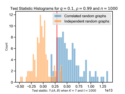
Figure 2: The histograms of the approximate tree counting statistic $Y_{{\mathcal{T}}}(A,B)$ (31) for $K=7$ and $t=1000$ random colorings over $100$ pairs of graphs, where the orange one corresponds to the independent model, the blue one corresponds to the correlated model, and the red line indicates the detection threshold.

To compare the performance of our test statistic under different settings, We also plot the Receiver Operating Characteristic (ROC) curves by varying detection threshold and plotting the true positive rate (one minus Type-II error) against the false positive rate (Type-I error). For comparison, we also plot the ROC curve for the random classifier, which is simply the diagonal. Finally, we compute the area under the curve (AUC), which can be interpreted as the probability that the test statistic has a larger value for a pair of graphs drawn from the correlated model than that drawn from the independent model independently.

In Figure 3, for each plot, we fix $n=1000$, $K=6$, $t=1000$, and $q\in\{0.001,0.01,0.1,0.5\}$, and vary $\rho\in\{0.8,0.85,0.9,0.95,0.99\}$. We observe that as $\rho$ increases, the ROC curve is moving toward the upper left corner and the AUC increases, demonstrating that our test statistic has improving performance. Moreover, as evident in the mean and variance calculation in Proposition 1, we need $\rho\geq|{\mathcal{T}}|^{-\frac{1}{2K}}\approx 0.82$ in order for the signal-to-noise ratio to exceed one, as there are in total $|{\mathcal{T}}|=11$ non-isomorphic trees with $K=6$ edges. Nevertheless, Figure 3 shows that our test statistic still achieves non-trivial power even when $\rho=0.8$ is close to this threshold. Recall from Theorem 1 that the smallest $\rho$ our test statistic can hope to achieve is $\lim_{K\to\infty}|{\mathcal{T}}|^{-\frac{1}{2K}}=\sqrt{\alpha}\approx 0.581$ where $\alpha\approx 0.338$ is Otter’s constant. Getting close to this threshold is computationally prohibitive as this convergence is rather slow: For $K=35$, $|{\mathcal{T}}|^{-\frac{1}{2K}}$ is still over $0.65$, at which case the number of unlabeled trees exceeds six trillion. (See [OEI] for a list of values for $|{\mathcal{T}}|$.)

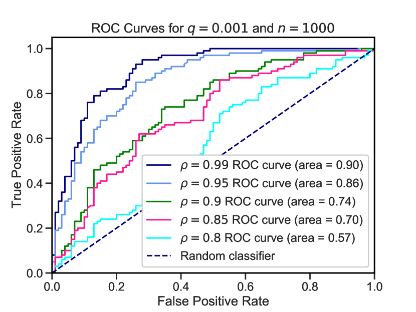
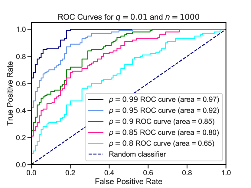
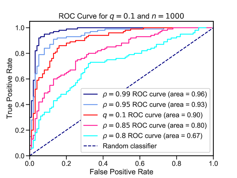
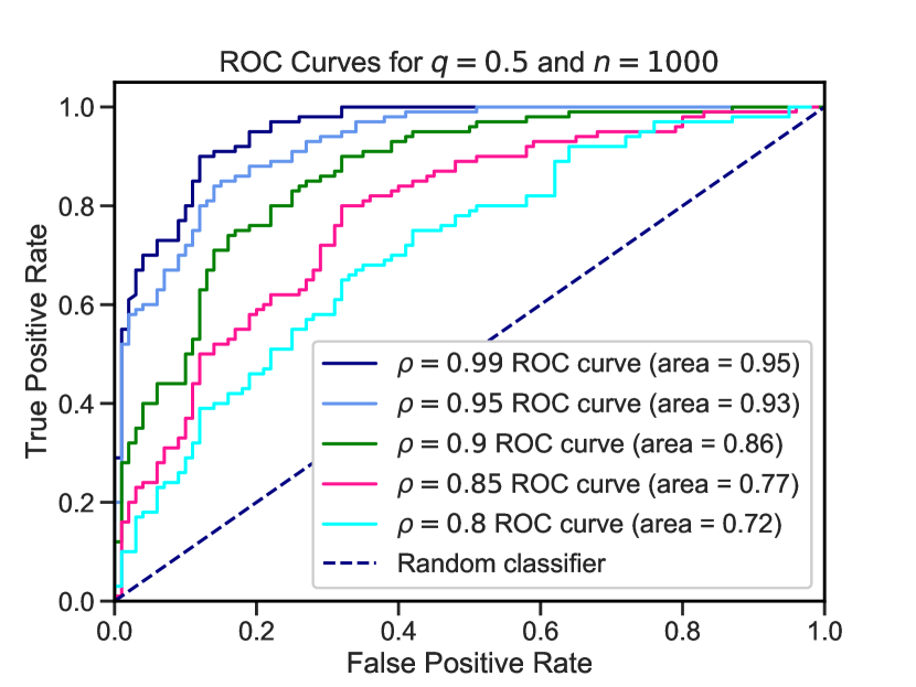
Figure 3: Comparison of the proposed test statistic for fixed edge probability $q$ and varying correlation parameter $\rho$.

In Figure 4, we vary the edge density $q\in\{0.001,0.01,0.1,0.5\}$. We observe that our test statistic performs well for a wide range of graph sparsity, except that when $q=0.001$, the performance slightly degrades. This is consistent with the theoretical results, showing that our test statistic works as long as the graphs are not overly sparse.

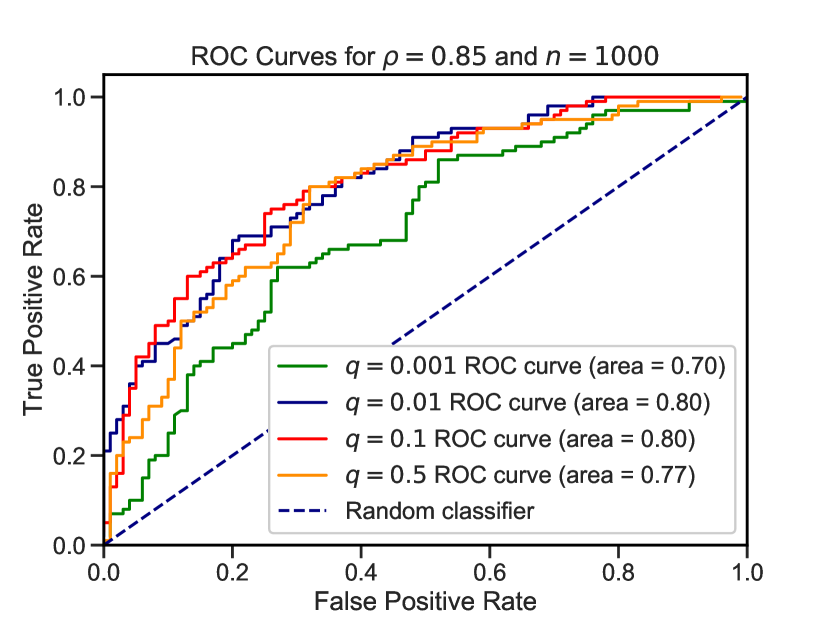
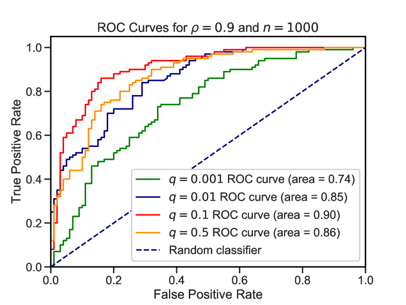
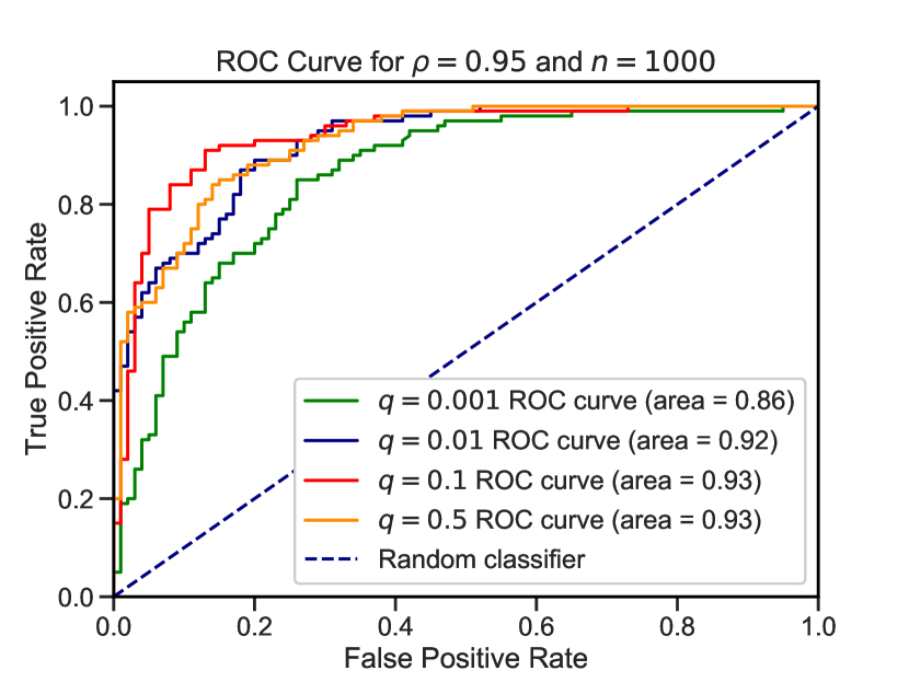
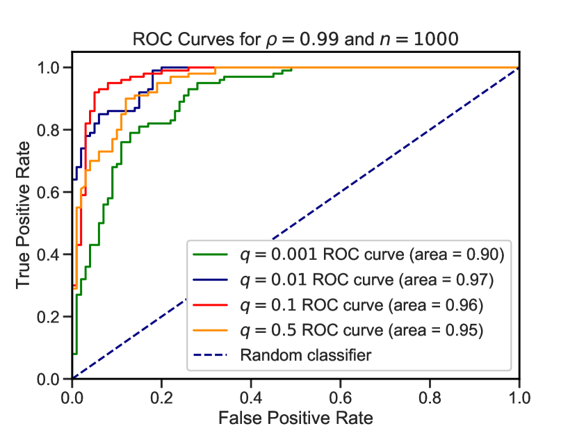
Figure 4: Comparison of the proposed test statistic for fixed correlation parameter $\rho$ and varying edge probability $q$.

In Figure 5(a), we fix $n=1000$, $q=0.1$, $\rho=0.95$, and $t=1000$, and vary the tree size $K\in\{2,3,4,5,6,7\}$. The performance of our test statistic is seen to improve significantly as $K$ increases. In Figure 5(b), we plot the median running time of Algorithm 1 on a pair of random graphs for each $K\in\{2,3,4,5,6,7\}$ when $t=1000$. We observe that the running time increases gradually up to $K=5$ and then rapidly afterwards. This shows a trade-off between the statistical performance and the computational complexity as $K$ varies.

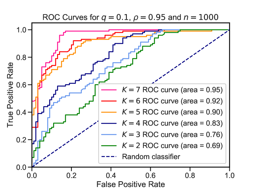
(a) ROC curves and AUC value.

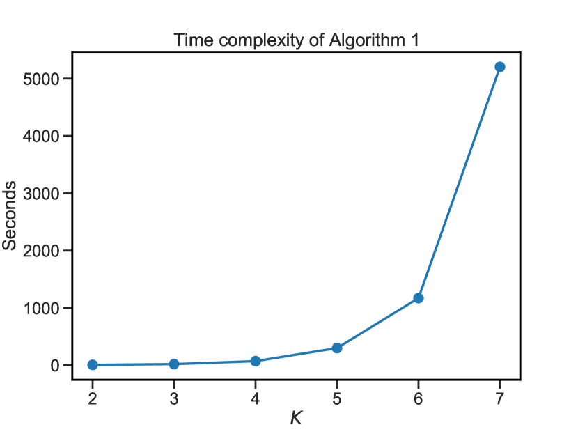
(b) Median running time of Algorithm 1 on a single pair of random graphs.

Figure 5: Comparison of statistical performance and time complexity of the proposed test statistic with $n=1000$, $q=0.1$, $\rho=0.95$, $t=1000$, and varying tree size $K\in\{2,3,4,5,6,7\}$.

Finally, we compare our test statistic with a heuristic variant that is more scalable to large sparse graphs. In particular, instead of first centering the adjacency matrices and counting the signed trees as per (3), we count the trees in the unweighted graphs in the usual sense and then subtract their means. This gives rise to the following statistic:

$$g_{\mathcal{T}}(A,B) \beta\triangleq\sum_{[H]\in{\mathcal{T}}}\mathsf{aut}(H)\left(W_{H}(A)-\gamma_{H}\right)\left(W_{H}(B)-\gamma_{H}\right),$$ (38)

where $\beta$ is in (4) and $\gamma_{H}\triangleq\mathbb{E}\left[W_{H}(A)\right]=\mathbb{E}\left[W_{H}(B)\right]=\frac{\binom{n}{K+1}(K+1)!}{\mathsf{aut}(H)}q^{K}$. Note that the form of $g_{\mathcal{T}}(A,B)$ resembles the test statistic in [BCL⁺19] as mentioned in Section 1.2, but with two crucial differences: (a) We restrict our attention to trees as opposed to strictly balanced graphs considered in [BCL⁺19]; (b) The weight in (38) for each $H$ is proportional to its number of automorphisms. Now, analogous to $f_{{\mathcal{T}}}(A,B)$, we approximately compute $g_{{\mathcal{T}}}(A,B)$ via color coding. Specifically, we generate $2t$ random coloring $\{\mu_{i}\}_{i=1}^{t}$ and $\{\nu_{i}\}_{i=1}^{t}$ that map $[n]$ to $[K+1]$, and define

$$Z_{\mathcal{T}}(A,B) \triangleq\sum_{[H]\in{\mathcal{T}}}\mathsf{aut}(H)\left(\frac{1}{t}\sum_{i=1}^{t}X_{H}(A,\mu_{i})-\gamma_{H}\right)\left(\frac{1}{t}\sum_{j=1}^{t}X_{H}(B,\nu_{j})-\gamma_{H}\right)\,,$$

which provides an unbiased estimator for $g_{\mathcal{T}}(A,B)$ as

$$\mathbb{E}\left[Z_{\mathcal{T}}(A,B)|A,B\right]=\frac{r^{2}}{\beta}g_{\mathcal{T}}(A,B)\,.$$

It turns out that the time complexity for computing $Z_{\mathcal{T}}(A,B)$ significantly improves since we work with unweighted sparse graphs as opposed to weighted dense graphs due to centering. To see this, to compute each $X_{H}(A,\mu)$, in the dynamic programming procedure (see (34) in Algorithm 2), for every $x\in[n]$, we only need to enumerate the neighbors of $x$ rather than all nodes. Thus, the time complexity for computing $X_{H}(A,\mu)$ becomes $O(mK3^{K})$, where $m$ is the number of edges in $A$. This significantly speeds up the computation when $m\ll n^{2}$.

In Figure 6, we consider a larger but sparser instance with $n=10000$, $q=0.0001$, $\rho=0.99$, and $t=1000$, and plot the ROC curve and compute the AUC for $Z_{\mathcal{T}}(A,B)$ when $K$ ranges from $2$ to $8$ respectively. We observe that the performance of $Z_{\mathcal{T}}(A,B)$ gets slightly better as $K$ increases from $2$ to $5$; however, even if $K$ is as large as $8$, it still falls short of $Y_{\mathcal{T}}(A,B)$ for $K=6$. This goes to show the importance of counting signed trees in the proposed test statistic. Computationally, $Z_{{\mathcal{T}}}(A,B)$ is much faster to compute than $Y_{{\mathcal{T}}}(A,B)$ (600x speedup when $K=6$).

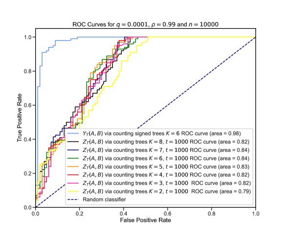
Figure 6: Comparison of performance of $Y_{\mathcal{T}}(A,B)$ when $K=6$, and $Z_{\mathcal{T}}(A,B)$ when $K$ ranges from $2$ to $8$, with $n=10000$, $q=0.0001$, $\rho=0.99$, and $t=1000$.

Appendix A Preliminary facts about graphs

Lemma 3.

Let $S,T$ be edge-induced subgraphs of $K_{n}$.

1. Suppose $S\cong T\cong H$ for some graph $H$. Let $\pi$ denote the random permutation uniformly distributed over ${\mathcal{S}}_{n}$. We have

   $$\mathbb{P}\left(\pi(S)=T\right)=\frac{1}{\mathsf{sub}_{n}(H)}=\frac{\mathsf{aut}(H)(n-|V(H)|)!}{n!}\leq\left(\frac{|V(H)|}{n}\right)^{|V(H)|}.$$

2. $V(S\Delta T)\cup\left(V(S)\cap V(T)\right)=V(S)\cup V(T)$, and $|V(S\Delta T)|+|V(S)\cap V(T)|=|V(S)\cup V(T)|+|V(S\Delta T)\cap V(S)\cap V(T)|$.

3. $V(S\cup T)=V(S)\cup V(T)$ and $V(S\cap T)\subset V(S)\cap V(T)$.

4. Suppose $S$ and $T$ are connected and $|V(S)\cap V(T)|\geq 1$. Then for any $E\subset S\cap T$,

   $$\left|V(S\Delta T)\cup E)\right| \geq|V(S)|+|V(T)|-2|V(S)\cap V(T)|+|V(E)|+{\mathbf{1}_{\left\{{E=\emptyset,S\neq T}\right\}}}.$$

5. For any graphs $H$ and $I$, for any $0\leq k\leq\min\{|V(H)|,|V(I)|\}$,

   $$\sum_{S\cong H}\sum_{T\cong I}{\mathbf{1}_{\left\{{|V(S)\cap V(T)|=k}\right\}}}\leq\binom{|V(H)|}{k}\binom{|V(I)|}{k}k!n^{|V(H)|+|V(I)|-k}.$$

Proof.

1. Note that $\pi(S)$ is uniformly distributed over the set $\{S^{\prime}\subset K_{n}:S^{\prime}\cong H\}$, whose cardinality is $\mathsf{sub}_{n}(H)=\mathsf{sub}(H,K_{n})$. Then $\mathbb{P}\left\{\pi(S)=T\right\}=\frac{1}{\mathsf{sub}_{n}(H)}$. Applying (2) yields

   $$\mathbb{P}\left(\pi(S)=T\right)=\frac{\mathsf{aut}(H)(n-|V(H)|)!}{n!}\leq\frac{|V(H)|!(n-|V(H)|)!}{n!}\leq\left(\frac{|V(H)|}{n}\right)^{|V(H)|},$$

   where the last inequality holds since $\binom{n}{k}\geq\left(\frac{n}{k}\right)^{k}$.

2. We remind the reader that in the sequel $S\cup T,S\cap T$ and $S\Delta T$ are edge-induced subgraphs of $K_{n}$. Since $V(S\Delta T)\subset V(S)\cup V(T)$ and $V(S)\cap V(T)\subset V(S)\cup V(T)$, we have $V(S\Delta T)\cup\left(V(S)\cap V(T)\right)\subset V(S)\cup V(T).$ Next, we show $V(S)\cup V(T)\subset V(S\Delta T)\cup\left(V(S)\cap V(T)\right).$ It suffices to show that $V(S)\Delta V(T)\subset V(S\Delta T)$. Indeed, for any $i\in V(S)\cap V(T)^{c}$, there exists some $j\in V(S)$ such that $(i,j)\in S\cap T^{c}$. Similarly, for any $i\in V(T)\cap V(S)^{c}$, there exists some $j\in V(T)$ such that $(i,j)\in T\cap S^{c}$. Then, $V(S\Delta T)\cup\left(V(S)\cap V(T)\right)=V(S)\cup V(T)$, which implies that $|V(S\Delta T)|+|V(S)\cap V(T)|=|V(S)\cup V(T)|+|V(S\Delta T)\cap\left(V(S)\cap V(T)\right)|.$

3. By definition, we have $V(S\cup T)=V(S)\cup V(T)$, and $V(S\cap T)\subset V(S)\cap V(T)$ follows because for any $i\in V(S\cap T)$, there exists some $j$ such that $(i,j)\in S\cap T$ and thus $i\in V(S)\cap V(T)$.

4. For $E\subset S\cap T$, we have

   $$\left|V\left((S\Delta T)\cup E\right)\right|=|V(S\Delta T)\cup V(E)|=|V(S\Delta T)|+|V(E)|-|V(S\Delta T)\cap V(E)|$$

   where the first equality applies part (iii). Furthermore, it follows from part (ii) that $|V(S\Delta T)|=|V(S)|+|V(T)|-2|V(S)\cap V(T)|+|V(S\Delta T)\cap\left(V(S)\cap V(T)\right)|$. Thus

   $$\left|V\left((S\Delta T)\cup E\right)\right| =|V(S)|+|V(T)|-2|V(S)\cap V(T)|+|V(E)|$$

   $$~{}~{}~{}~{}+|V(S\Delta T)\cap\left(V(S)\cap V(T)\right)|-|V(S\Delta T)\cap V(E)|$$ (39)

   $$\geq|V(S)|+|V(T)|-2|V(S)\cap V(T)|+|V(E)|,$$

   where the last step follows from $V(E)\subset V(S)\cap V(T)$ since $E\subset S\cap T$.

   It remains to consider the special case of $E\neq\emptyset$ and $S\neq T$. Continuing (39), it suffices to verify that $|V(S\Delta T)\cap\left(V(S)\cap V(T)\right)|\geq 1$. Consider two cases.

   • Suppose that $S\cap T\neq\emptyset$. By assumption, $|V(S)\cap V(T)|\geq 1$ and $S,T$ are connected. Thus $S\cup T$ is also connected. Then $V(S\Delta T)\cap V(S\cap T)\neq\emptyset$, and

     $$|V(S\Delta T)\cap\left(V(S)\cap V(T)\right)|\geq|V(S\Delta T)\cap V(S\cap T)|\geq 1\,,$$

     where the first inequality holds by part (iii).

   • Suppose that $S\cap T=\emptyset$, then $S\cup T=S\Delta T$ and $V(S\Delta T)=V(S)\cup V(T)$ by part (iii). Thus,

     $$|V(S\Delta T)\cap\left(V(S)\cap V(T)\right)|=|V(S)\cap V(T)|\geq 1\,,$$

     where the last inequality holds by our standing assumption that $|V(S)\cap V(T)|\geq 1$.

   This concludes the proof of part (iv).

5. We have

   $$\sum_{S\cong H}\sum_{T\cong I}{\mathbf{1}_{\left\{{|V(S)\cap V(T)|=k}\right\}}}$$

   $$\leq\binom{n}{|V(H)|}\binom{|V(H)|}{k}\binom{n-|V(H)|}{|V(I)|-k}|V(H)|!|V(I)|!$$

   $$=\frac{n!}{(n-|V(H)|)!}\frac{(n-|V(H)|)!}{(n-|V(H)|-|V(I)|+k)!}\binom{|V(H)|}{k}\binom{|V(I)|}{k}k!$$

   $$\leq\binom{|V(H)|}{k}\binom{|V(I)|}{k}k!n^{|V(H)|+|V(I)|-k}\,.$$

∎

Appendix B Postponed proofs in Section 3

B.1 Proof of Proposition 2

By the discussion in Section 3.3, it suffices to bound the two terms (27) and (28).

Bounding term (I). Recall from (14) that $\left\langle L,\phi_{\mathsf{S}}\right\rangle=a_{H}$ and by definition $a_{H}\mathsf{sub}_{n}(H)=\rho^{|E(H)|}=\rho^{K}$ for all $H\in{\mathcal{H}}$. Then

$$\mathbb{E}_{\mathcal{P}}[f_{\mathcal{H}}]=|{\mathcal{H}}|\rho^{2K}.$$ (40)

Therefore, applying (22) in Lemma 1 yields that

(I) $$\leq\sum_{[H]\in{\mathcal{H}}}a_{H}\sum_{[I]\in{\mathcal{H}}}a_{I}\sum_{S_{1}\cong H}\sum_{S_{2}\cong H}\sum_{T_{1}\cong I}\sum_{T_{2}\cong I}a_{H}a_{I}\left(\gamma\left(1+{\mathbf{1}_{\left\{{H\cong I}\right\}}}\right)-1\right)$$

$$=\sum_{[H]\in{\mathcal{H}}}a_{H}^{2}\sum_{[I]\in{\mathcal{H}}}a_{I}^{2}\mathsf{sub}_{n}(H)^{2}\mathsf{sub}(I)^{2}\left(\gamma\left(1+{\mathbf{1}_{\left\{{H\cong I}\right\}}}\right)-1\right)$$

$$=\left(\gamma-1\right)\left(\sum_{[H]\in{\mathcal{H}}}a_{H}^{2}\mathsf{sub}_{n}(H)^{2}\right)^{2}+\gamma\sum_{[H]\in{\mathcal{H}}}a_{H}^{4}\mathsf{sub}_{n}(H)^{4}$$

$$=|{\mathcal{H}}|^{2}\rho^{4K}\left(\gamma-1\right)+|{\mathcal{H}}|\rho^{4K}\gamma\,.$$

Recall $\gamma=\exp\left(\frac{M^{2}}{n-2M+1}\right)$. In view of the definition (20), by choosing $J$ to be a single vertex we have $\Phi_{H}\leq n$ and hence $\Phi_{{\mathcal{H}}}\leq n$. Thus, by the assumption (21), we have $M=o(\log n)$. Thus $\gamma=1+o(1)$. Moreover, by (19), $|{\mathcal{H}}|=\omega(\rho^{-2K})=\omega(1)$. It follows that

$$\frac{\text{(I)}}{\left(\mathbb{E}_{\mathcal{P}}\left[f_{\mathcal{H}}\right]\right)^{2}}\leq\left(\gamma-1\right)+|{\mathcal{H}}|^{-1}\gamma=o(1).$$ (41)

Bounding term (II). For any $S,T\subset\binom{[n]}{2}$, define

$$\ell(S,T)\triangleq\left(\frac{2M}{n}\right)^{-|V(S)\cap V(T)|}h(S,T)\,.$$ (42)

In the sequel, we will need the following auxiliary result.

Lemma 4.

For any $H,I$ in ${\mathcal{H}}$ with $K$ edges and at most $M$ vertices,

$$\sum_{S\cong H}\sum_{T\cong I}\ell(S,T){\mathbf{1}_{\left\{{|V(S)\cap V(T)|\geq 1}\right\}}}\leq n^{|V(H)|+|V(I)|}b_{K},$$

where

$$b_{K}\triangleq\frac{2^{K}(2M)^{\frac{M}{2}}2^{M}}{\sqrt{\Phi_{{\mathcal{H}}}}}\,,$$

where $\Phi_{\mathcal{H}}=\min_{H\in{\mathcal{H}}}\Phi_{H}$ is defined in Proposition 2 – see (20).

Proof of Lemma 4.

By (26),

$$\sum_{S\cong H}\sum_{T\cong I}\ell(S,T){\mathbf{1}_{\left\{{|V(S)\cap V(T)|\geq 1}\right\}}} \leq\frac{2^{K}(2M)^{\frac{M}{2}}}{\sqrt{\Phi_{{\mathcal{H}}}}}\sum_{S\cong H}\sum_{T\cong I}\left(\frac{2M}{n}\right)^{-|V(S)\cap V(T)|}{\mathbf{1}_{\left\{{|V(S)\cap V(T)|\geq 1}\right\}}}.$$ (43)

Now, in view of Lemma 3(v), we have that

$$\sum_{S\cong H}\sum_{T\cong I}{\mathbf{1}_{\left\{{|V(S)\cap V(T)|=k}\right\}}}\leq\binom{|V(H)|}{k}\binom{|V(I)|}{k}k!n^{|V(H)|+|V(I)|-k}\,;$$

Therefore,

$$\sum_{S\cong H}\sum_{T\cong I}\left(\frac{2M}{n}\right)^{-|V(S)\cap V(T)|}{\mathbf{1}_{\left\{{|V(S)\cap V(T)|\geq 1}\right\}}}$$

$$\leq\sum_{k=1}^{|V(H)|}\sum_{S\cong H}\sum_{T\cong I}{\mathbf{1}_{\left\{{|V(S)\cap V(T)|=k}\right\}}}\left(\frac{2M}{n}\right)^{-k}$$

$$\leq\sum_{k=1}^{|V(H)|}\binom{|V(H)|}{k}\binom{|V(I)|}{k}k!n^{|V(H)|+|V(I)|-k}\left(\frac{2M}{n}\right)^{-k}$$

$$\leq 2^{M}n^{|V(H)|+|V(I)|}\,,$$

where the last inequality holds because

$$\sum_{k=1}^{|V(H)|}\binom{|V(H)|}{k}\binom{|V(I)|}{k}k!\left(2M\right)^{-k} \leq\sum_{k=1}^{|V(H)|}\binom{|V(H)|}{k}M^{k}\left(2M\right)^{-k}$$

$$=\sum_{k=1}^{|V(H)|}\binom{|V(H)|}{k}2^{-k}\leq 2^{M}\,.$$

The proof is completed by combining the last display with (43). ∎

Now, let us return to the proof of Proposition 2. Fix any $H,I\in{\mathcal{H}}$. Fix ${\mathsf{S}}=(S_{1},S_{2})$ and ${\mathsf{T}}=(T_{1},T_{2})$ such that $S_{1}\cong S_{2}\cong H$ and $T_{1}\cong T_{2}\cong I$, and $|V(S_{1}\cap T_{1})|\geq 1,|V(S_{2}\cap T_{2})|\geq 1$. Applying (24) in Lemma 1 yields that

$$\left\langle L,\phi_{\mathsf{S}}\phi_{\mathsf{T}}\right\rangle{\mathbf{1}_{\left\{{\left\langle L,\phi_{\mathsf{S}}\phi_{\mathsf{T}}\right\rangle\geq 0}\right\}}}$$

$$\leq\left(\frac{2M}{n}\right)^{|V(H)|+|V(I)|-|V(S_{1})\cap V(T_{1})|-|V(S_{2})\cap V(T_{2})|}\biggl{\{}{\mathbf{1}_{\left\{{{\mathsf{S}}={\mathsf{T}}}\right\}}}+h(S_{2},T_{2}){\mathbf{1}_{\left\{{S_{1}=T_{1}}\right\}}}$$

$$~{}~{}~{}~{}+h(S_{1},T_{1}){\mathbf{1}_{\left\{{S_{2}=T_{2}}\right\}}}+h(S_{1},T_{1})h(S_{2},T_{2})\biggr{\}}$$

$$={\mathbf{1}_{\left\{{{\mathsf{S}}={\mathsf{T}}}\right\}}}+\left(\frac{2M}{n}\right)^{|V(H)|}\ell(S_{1},T_{1}){\mathbf{1}_{\left\{{S_{2}=T_{2}}\right\}}}+\left(\frac{2M}{n}\right)^{|V(H)|}\ell(S_{2},T_{2}){\mathbf{1}_{\left\{{S_{1}=T_{1}}\right\}}}+$$

$$~{}~{}~{}~{}\left(\frac{2M}{n}\right)^{|V(H)|+|V(I)|}\ell(S_{1},T_{1})\ell(S_{2},T_{2})\,.$$ (44)

Combining (44) with Lemma 4 yields that

$$\sum_{S_{1}\cong H}\sum_{S_{2}\cong H}\sum_{T_{1}\cong I}\sum_{T_{2}\cong I}\left\langle L,\phi_{\mathsf{S}}\phi_{\mathsf{T}}\right\rangle{\mathbf{1}_{\left\{{\left\langle L,\phi_{\mathsf{S}}\phi_{\mathsf{T}}\right\rangle\geq 0}\right\}}}\cdot{\mathbf{1}_{\left\{{|V(S_{1}\cap T_{1})|\geq 1,\,|V(S_{2}\cap T_{2})|\geq 1}\right\}}}$$

$$\leq\sum_{S_{1}\cong H}\sum_{S_{2}\cong H}\sum_{T_{1}\cong I}\sum_{T_{2}\cong I}\biggl{\{}{\mathbf{1}_{\left\{{{\mathsf{S}}={\mathsf{T}}}\right\}}}+\left(\frac{2M}{n}\right)^{|V(H)|}\ell(S_{1},T_{1}){\mathbf{1}_{\left\{{S_{2}=T_{2}}\right\}}}+$$

$$~{}~{}~{}~{}\left(\frac{2M}{n}\right)^{|V(H)|}\ell(S_{2},T_{2}){\mathbf{1}_{\left\{{S_{1}=T_{1}}\right\}}}+\left(\frac{2M}{n}\right)^{|V(H)|+|V(I)|}\ell(S_{1},T_{1})\ell(S_{2},T_{2})\biggr{\}}$$

$$~{}~{}~{}~{}{\mathbf{1}_{\left\{{|V(S_{1}\cap T_{1})|\geq 1,\,|V(S_{2}\cap T_{2})|\geq 1}\right\}}}$$

$$\leq\mathsf{sub}_{n}(H)^{2}{\mathbf{1}_{\left\{{H\cong I}\right\}}}+2\mathsf{sub}_{n}(H)\left(2M\right)^{M}n^{|V(H)|}b_{K}{\mathbf{1}_{\left\{{H\cong I}\right\}}}+$$

$$~{}~{}~{}~{}\left(2M\right)^{2M}n^{|V(H)|+|V(I)|}b_{K}^{2}\,.$$ (45)

Define

$$c_{K} \triangleq\rho^{-2K}2^{2M}M^{4M}b_{K}^{2}=\frac{\rho^{-2K}M^{5M}2^{5M+2K+2}}{\Phi_{{\mathcal{H}}}}\,.$$

Summing over $H,I\in{\mathcal{H}}$, it follows from (45) that

(II) $$\leq\sum_{[H]\in{\mathcal{H}}}a_{H}\sum_{[I]\in{\mathcal{H}}}a_{I}\biggl{\{}(\mathsf{sub}_{n}(H)^{2}{\mathbf{1}_{\left\{{H\cong I}\right\}}}+2\mathsf{sub}_{n}(H)\left(2M\right)^{M}n^{|V(H)|}b_{K}{\mathbf{1}_{\left\{{H\cong I}\right\}}}+$$

$$~{}~{}~{}~{}\left(2M\right)^{2M}n^{|V(H)|+|V(I)|}b_{K}^{2}\biggr{\}}$$

$$=\sum_{[H]\in{\mathcal{H}}}a_{H}^{2}\left(\mathsf{sub}_{n}(H)^{2}+2\mathsf{sub}_{n}(H)\left(2M\right)^{M}n^{|V(H)|}b_{K}\right)+\left(\sum_{[H]\in{\mathcal{H}}}a_{H}\left(2M\right)^{M}n^{|V(H)|}b_{K}\right)^{2}$$

$$\overset{(a)}{=}\sum_{[H]\in{\mathcal{H}}}\left(\rho^{2K}+2a_{H}\rho^{K}\left(2M\right)^{M}n^{|V(H)|}b_{K}\right)+\left(\sum_{[H]\in{\mathcal{H}}}a_{H}\left(2M\right)^{M}n^{|V(H)|}b_{K}\right)^{2}$$

$$\overset{(b)}{\leq}|{\mathcal{H}}|\rho^{2K}\left(1+2\rho^{K}\sqrt{c_{K}}\right)+|{\mathcal{H}}|^{2}\rho^{4K}c_{K},$$

where $(a)$ holds as $a_{H}\mathsf{sub}_{n}(H)=\rho^{|E(H)|}=\rho^{K}$; $(b)$ holds by Lemma 3(i) as $a_{H}\leq\rho^{K}\left(\frac{M}{n}\right)^{|V(H)|}$ and $|V(H)|\leq M$ for all $H\in{\mathcal{H}}$. Then, using (40), we have

$$\frac{\text{(II)}}{\left(\mathbb{E}_{{\mathcal{P}}}[f_{{\mathcal{H}}}]\right)^{2}} \leq\left(|{\mathcal{H}}|\rho^{2K}\right)^{-1}\left(1+2\rho^{K}\sqrt{c_{K}}\right)+c_{K}=o(1)\,,$$ (46)

where the equality holds because $|{\mathcal{H}}|\rho^{2K}=\omega(1)$ by (19) and $c_{K}=o(1)$ by (21). Hence, combining (41) and (46), we obtain the desired result

$$\mathrm{Var}_{{\mathcal{P}}}[f_{{\mathcal{H}}}]=o\left(\left(\mathbb{E}_{{\mathcal{P}}}[f_{{\mathcal{H}}}]\right)^{2}\right)\,.$$

Finally, it remains to show that in the special case of trees, namely ${\mathcal{H}}={\mathcal{T}}$ and $M=K+1$, the condition (7) ensures that ${\mathcal{T}}$ satisfies both (19) and (21). By (37), under the assumption that $\rho^{2}>\alpha$ and $K=\omega(1)$, we get (19). Moreover, for any tree $H\in{\mathcal{T}}$ and any subgraph $J\subset H$, $J$ must be a forest and hence satisfies $|V(J)|\geq|E(J)|+1$. Thus

$$\Phi_{H}=\min_{J\subset H,|V(J)|\geq 1}n^{|V(J)|}q^{|E(J)|}=\begin{cases}n^{K+1}q^{K}&\text{ if }nq<1\\ n&\text{ if }nq\geq 1\end{cases}\,$$

and by definition $\Phi_{\mathcal{T}}=\Phi_{H}$.

Under the condition (7), we have $K\leq\frac{\log n}{2\log(\frac{1}{nq})}$ and hence $n^{K+1}q^{K}\geq\sqrt{n}$. Therefore $\Phi_{H}\geq\sqrt{n}$. Moreover, (7) also implies that $K\leq\frac{\log n}{16\log\log n}$. Since $\rho^{2}>\alpha>1/4$, the desired (21) follows from

$$\rho^{-2K}(K+1)^{5K+5}2^{7K+5}\leq 2^{9K+5}(K+1)^{5K+5}=o(\sqrt{n})\,.$$

B.2 Proof of Lemma 1

Fix ${\mathsf{S}}=(S_{1},S_{2})$ and ${\mathsf{T}}=(T_{1},T_{2})$ such that $S_{1}\cong S_{2}\cong H$ and $T_{1}\cong T_{2}\cong I$ where $H$ and $I$ that are connected graphs with $K$ edges and at most $M$ vertices.

Case (i): $V(S_{1})\cap V(T_{1})=\emptyset$ and $V(S_{2})\cap V(T_{2})=\emptyset$. In this case, we have $S_{1}\cap T_{1}=\emptyset$ and $S_{2}\cap T_{2}=\emptyset$. By change of measure and the definition of $\phi_{\mathsf{S}}$ given in (10), we get that

$$\left\langle L,\phi_{\mathsf{S}}\phi_{\mathsf{T}}\right\rangle =\mathbb{E}_{{\mathcal{P}}}\left[\phi_{\mathsf{S}}(A,B)\phi_{\mathsf{T}}(A,B)\right]$$

$$=\mathbb{E}_{\pi}\mathbb{E}_{{\mathcal{P}}|\pi}\left[\sigma^{-2(|E(H)|+|E(I)|)}\prod_{(i,j)\in S_{1}\cup T_{1}}\overline{A}_{ij}\prod_{(k,\ell)\in S_{2}\cup T_{2}}\overline{B}_{k,\ell}\right]$$

$$=\rho^{|E(H)|+|E(I)|}\mathbb{P}\left(\pi(S_{1}\cup T_{1})=S_{2}\cup T_{2}\right)$$

$$=a_{H}a_{I}\frac{\mathbb{P}\left(\pi(S_{1}\cup T_{1})=S_{2}\cup T_{2}\right)}{\mathbb{P}\left(\pi(S_{1})=S_{2}\right)\mathbb{P}\left(\pi(T_{1})=T_{2}\right)}.$$ (47)

Suppose $\pi(S_{1}\cup T_{1})=S_{2}\cup T_{2}$. Since $V(S_{1})\cap V(T_{1})=\emptyset$, $\pi(V(S_{1}))\cap\pi(V(T_{1}))=\emptyset$. Since $S_{1}\cong S_{2}\cong H$ and $T_{1}\cong T_{2}\cong I$ where $H$ and $I$ that are connected graphs, given $\pi(V(S_{1}))\cap\pi(V(T_{1}))=\emptyset$ and $V(S_{2})\cap V(T_{2})=\emptyset$, we must have either $\pi(S_{1})=S_{2}$ and $\pi(T_{1})=T_{2}$, or $\pi(S_{1})=T_{2}$ and $\pi(T_{2})=S_{2}$. Hence,

$$\mathbb{P}\left(\pi(S_{1}\cup T_{1})=S_{2}\cup T_{2}\right) =\mathbb{P}\left(\pi(S_{1})=S_{2},\pi(T_{1})=T_{2}\right)+\mathbb{P}\left(\pi(S_{1})=T_{2},\pi(S_{1})=T_{2}\right){\mathbf{1}_{\left\{{H\cong I}\right\}}}$$

$$=\mathbb{P}\left(\pi(S_{1})=S_{2},\pi(T_{1})=T_{2}\right)\left(1+{\mathbf{1}_{\left\{{H\cong I}\right\}}}\right).$$

Note that

$$\mathbb{P}\left(\pi(S_{1})=S_{2},\pi(T_{1})=T_{2}\right)=\frac{(n-|V(H)|-|V(I)|)!\mathsf{aut}(H)\mathsf{aut}(I)}{n!}\,.$$

Since $\mathbb{P}\left(\pi(S_{1})=S_{2}\right)=\frac{(n-|V(H)|)!\mathsf{aut}(H)}{n!}$ and $\mathbb{P}\left(\pi(T_{1})=T_{2}\right)=\frac{(n-|V(I)|)!\mathsf{aut}(I)}{n!}$, we have

$$\frac{\mathbb{P}\left(\pi(S_{1})=S_{2},\pi(T_{1})=T_{2}\right)}{\mathbb{P}\left(\pi(S_{1})=S_{2}\right)\mathbb{P}\left(\pi(T_{1})=T_{2}\right)} =\frac{n!(n-|V(H)|-|V(I)|)!}{(n-|V(I)|)!(n-|V(H)|)!}$$

$$\overset{(a)}{\leq}\exp\left(\frac{|V(H)||V(I)|}{n-|V(H)|-|V(I)|+1}\right)$$

$$\overset{(b)}{\leq}\gamma\,,$$ (48)

where $(a)$ holds because for any $\ell,m\in{\mathbb{N}}$ such that $\ell+m\leq n$,

$$\frac{n!(n-\ell-m)!}{(n-\ell)!(n-m)!}=\prod_{k=n-\ell+1}^{n}\frac{k}{k-m}\leq\left(\frac{n-\ell+1}{n-\ell-m+1}\right)^{\ell}\leq\exp\left(\frac{\ell m}{n-\ell-m+1}\right),$$

where the last inequality holds because for any $x\in{\mathbb{R}}$, $1+x\leq\exp(x)$; $(b)$ holds because $|V(H)|,|V(I)|\leq M$ and $\gamma\triangleq\exp\left(\frac{M^{2}}{n-2M+1}\right)$. Combining (47) and (48), we arrive at the desired bound:

$$0\leq\left\langle L,\phi_{\mathsf{S}}\phi_{\mathsf{T}}\right\rangle \leq a_{H}a_{I}\gamma\left(1+{\mathbf{1}_{\left\{{H\cong I}\right\}}}\right)\,.$$

Case (ii): $V(S_{1})\cap V(T_{1})=\emptyset$ and $V(S_{2})\cap V(T_{2})\neq\emptyset$, or $V(S_{1})\cap V(T_{1})\neq\emptyset$ and $V(S_{2})\cap V(T_{2})=\emptyset$. While this case itself is easy, we set up some notation for both Case 2 and Case 3 below. By change of measure,

$$\left\langle L,\phi_{\mathsf{S}}\phi_{\mathsf{T}}\right\rangle=\mathbb{E}_{{\mathcal{P}}}\left[\phi_{\mathsf{S}}(A,B)\phi_{\mathsf{T}}(A,B)\right]=\mathbb{E}_{\pi}\left[g(\pi)\right],$$ (49)

where

$$g(\pi) \triangleq\mathbb{E}_{{\mathcal{P}}|\pi}\left\{\sigma^{-2|E(H)|-2|E(I)|}\prod_{(i,j)\in S_{1}\cap T_{1}}\overline{A}_{ij}^{2}\prod_{(i,j)\in S_{1}\Delta T_{1}}\overline{A}_{ij}\prod_{(k,\ell)\in S_{2}\cap T_{2}}\overline{B}_{k,\ell}^{2}\prod_{(k,\ell)\in S_{2}\Delta T_{2}}\overline{B}_{k,\ell}\right\}.$$

Given a permutation $\pi$, we define

$$K_{11}\triangleq S_{1}\Delta T_{1}\cap\pi^{-1}\left(S_{2}\Delta T_{2}\right),\quad K_{12}\triangleq\left(S_{1}\Delta T_{1}\right)\cap\pi^{-1}\left(S_{2}\cap T_{2}\right)\,,$$

$$K_{21}\triangleq\left(S_{1}\cap T_{1}\right)\cap\pi^{-1}\left(S_{2}\Delta T_{2}\right),\quad K_{22}\triangleq\left(S_{1}\cap T_{1}\right)\cap\pi^{-1}\left(S_{2}\cap T_{2}\right)\,,$$

and

$$K_{20}\triangleq\left(S_{1}\cap T_{1}\right)\backslash\left(K_{21}\cup K_{22}\right),\quad K_{02}\triangleq\left(S_{2}\cap T_{2}\right)\backslash\left(K_{12}\cup K_{22}\right).$$

In the sequel, we will split the product in the definition of $g(\pi)$ according to the mutually exclusive sets $K_{\ell m}$ defined above, where $0\leq\ell,m\leq 2$ and $2\leq\ell+m\leq 4$. Note that, if there exists $(i,j)\in S_{1}\Delta T_{1}$ such that $\pi(i,j)\not\in S_{2}\cup T_{2}$, or if there exists $(k,\ell)\in S_{2}\Delta T_{2}$ such that $(k,\ell)\not\in\pi(S_{1}\cup T_{1})$, we have $g(\pi)=0$. Thus, by independence of the pairs $(A_{ij},B_{\pi(i)\pi(j)})$, we get

$$g(\pi) =\prod_{\begin{subarray}{c}2\leq\ell+m\leq 4\\ 0\leq\ell,m\leq 2\end{subarray}}\sigma^{-(\ell+m)|K_{\ell m}|}\prod_{(i,j)\in K_{\ell m}}\mathbb{E}_{{\mathcal{P}}|\pi}\left[\overline{A}_{ij}^{\ell}\overline{B}_{\pi(i)\pi(j)}^{m}\right]$$

$$~{}~{}~{}~{}\times{\mathbf{1}_{\left\{{S_{1}\Delta T_{1}=K_{11}\cup K_{12}}\right\}}}{\mathbf{1}_{\left\{{\pi^{-1}\left(S_{2}\Delta T_{2}\right)=K_{11}\cup K_{21}}\right\}}}.$$ (50)

Suppose that $|V(S_{1})\cap V(T_{1})|=0$ and $|V(S_{2})\cap V(T_{2})|\geq 1$. Then for any $\pi\in{\mathcal{S}}_{n}$, $\pi(S_{1}\Delta T_{1})\not\subset S_{2}\cup T_{2}$, because the former has $|V(S_{1})|+|V(T_{1})|$ vertices and the latter has fewer. As a result, $g(\pi)=0$ in view of (50). As a result, $\left\langle L,\phi_{\mathsf{S}}\phi_{\mathsf{T}}\right\rangle=0$. The case of $|V(S_{2})\cap V(T_{2})|=0$ and $|V(S_{1})\cap V(T_{1})|\geq 1$ is similar.

Case (iii): $|V(S_{1})\cap V(T_{1})|\geq 1$ and $|V(S_{2})\cap V(T_{2})|\geq 1$. Recall that in this case we assume $q\leq 1/2$. We continue to use the notation $g(\pi)$ and $K_{\ell m}$ introduced in Case (ii). Crucially, we need the following lemma, bounding the cross-moments of $\overline{A}_{ij}$ and $\overline{B}_{\pi(i)\pi(j)}$.

Lemma 5.

Assume $q\leq\frac{1}{2}$. For any $\pi\in{\mathcal{S}}_{n}$, $(i,j)\in\binom{[n]}{2}$, and $0\leq\ell,m\leq 2$ such that $2\leq\ell+m\leq 4$, we have

$$\left|\mathbb{E}_{{\mathcal{P}}|\pi}\left[\sigma^{-\ell-m}\overline{A}_{ij}^{\ell}\overline{B}_{\pi(i)\pi(j)}^{m}\right]\right|\leq{\mathbf{1}_{\left\{{\ell+m=2}\right\}}}+\sqrt{\frac{1}{q}}{\mathbf{1}_{\left\{{\ell+m=3}\right\}}}+\frac{1}{q}{\mathbf{1}_{\left\{{\ell+m=4}\right\}}}.$$

Proof of Lemma 5.

We split the proof into three cases according to the value of $\ell+m$.

• If $\ell+m=2$,

  $$\mathbb{E}_{{\mathcal{P}}|\pi}\left[\sigma^{-2}\overline{A}_{ij}^{2}\right] =\mathbb{E}_{{\mathcal{P}}|\pi}\left[\sigma^{-2}\overline{B}_{\pi(i)\pi(j)}^{2}\right]=1,$$

  and

  $$\left|\mathbb{E}_{{\mathcal{P}}|\pi}\left[\sigma^{-2}\overline{A}_{ij}\overline{B}_{\pi(i)\pi(j)}\right]\right|=|\rho|;$$

• If $\ell+m=3$,

  $$\mathbb{E}_{{\mathcal{P}}|\pi}\left[\sigma^{-3}\overline{A}_{ij}^{2}\overline{B}_{\pi(i)\pi(j)}\right] =\mathbb{E}_{{\mathcal{P}}|\pi}\left[\sigma^{-3}\overline{A}_{ij}\overline{B}_{\pi(i)\pi(j)}^{2}\right]=\frac{\rho(1-2q)}{\sqrt{q(1-q)}}\,.$$

  Given $q\leq\frac{1}{2}$ and $1-2q\leq 1-q$, we have that

  $$\left|\mathbb{E}_{{\mathcal{P}}|\pi}\left[\sigma^{-3}\overline{A}_{ij}^{2}\overline{B}_{\pi(i)\pi(j)}\right]\right|=\left|\mathbb{E}_{{\mathcal{P}}|\pi}\left[\sigma^{-3}\overline{A}_{ij}\overline{B}_{\pi(i)\pi(j)}^{2}\right]\right|\leq\sqrt{\frac{1}{q}}\,.$$

• If $\ell+m=4$, we have that

  $$\mathbb{E}_{{\mathcal{P}}|\pi}\left[\sigma^{-4}\bar{A}_{ij}^{2}\bar{B}_{\pi(i)\pi(j)}^{2}\right] =\frac{q^{2}(1-q)^{2}+\rho q(1-q)(1-2q)^{2}}{q^{2}(1-q)^{2}}$$

  $$=\frac{q(1-q)+\rho(1-2q)^{2}}{q(1-q)}\,.$$

  Since

  $$-1+q\leq q(1-q)-(1-2q)^{2}\leq q(1-q)+\rho(1-2q)^{2}\leq q(1-q)+(1-2q)^{2}\leq 1-q\,$$

  given $q\leq\frac{1}{2}$ and $-1\leq\rho\leq 1$, we have that

  $$\left|\mathbb{E}_{{\mathcal{P}}|\pi}\left[\sigma^{-4}\bar{A}_{ij}^{2}\bar{B}_{\pi(i)\pi(j)}^{2}\right]\right| \leq\frac{1}{q}\,.$$

Combining all the cases proves the lemma. ∎

Applying Lemma 5 to (50), we get that

$$g(\pi)\leq q^{-\frac{|K_{12}|+|K_{21}|+2|K_{22}|}{2}}{\mathbf{1}_{\left\{{S_{1}\Delta T_{1}=K_{11}\cup K_{12}}\right\}}}{\mathbf{1}_{\left\{{\pi^{-1}\left(S_{2}\Delta T_{2}\right)=K_{11}\cup K_{21}}\right\}}}\,.$$

Since

$${\mathbf{1}_{\left\{{S_{1}\Delta T_{1}=K_{11}\cup K_{12}}\right\}}}{\mathbf{1}_{\left\{{\pi^{-1}\left(S_{2}\Delta T_{2}\right)=K_{11}\cup K_{21}}\right\}}}\leq{\mathbf{1}_{\left\{{\pi\left(\left(S_{1}\Delta T_{1}\right)\cup K_{21}\cup K_{22}\right)=\left(S_{2}\Delta T_{2}\right)\cup\pi\left(K_{12}\cup K_{22}\right)}\right\}}}\,.$$

combining it with (49), we have

$$\left\langle L,\phi_{\mathsf{S}}\phi_{\mathsf{T}}\right\rangle \leq\mathbb{E}_{\pi}\left[q^{-\frac{|K_{12}|+|K_{21}|+2|K_{22}|}{2}}{\mathbf{1}_{\left\{{\pi\left(\left(S_{1}\Delta T_{1}\right)\cup K_{21}\cup K_{22}\right)=\left(S_{2}\Delta T_{2}\right)\cup\pi\left(K_{12}\cup K_{22}\right)}\right\}}}\right].$$

Since $K_{21}\cup K_{22}\subset S_{1}\cap T_{1}$, $\pi\left(K_{12}\cup K_{22}\right)\subset S_{2}\cap T_{2}$ for any $\pi\in{\mathcal{S}}_{n}$,

$$\left\langle L,\phi_{\mathsf{S}}\phi_{\mathsf{T}}\right\rangle \leq\mathbb{E}_{\pi}\left[\sum_{E_{1}\subset S_{1}\cap T_{1}}\sum_{E_{2}\subset S_{2}\cap T_{2}}q^{-\frac{|E_{1}|+|E_{2}|}{2}}{\mathbf{1}_{\left\{{\pi\left(\left(S_{1}\Delta T_{1}\right)\cup E_{1}\right)=\left(S_{2}\Delta T_{2}\right)\cup E_{2}}\right\}}}\right]$$

$$\leq\sum_{E_{1}\subset S_{1}\cap T_{1}}\sum_{E_{2}\subset S_{2}\cap T_{2}}q^{-\frac{|E_{1}|+|E_{2}|}{2}}\mathbb{P}\left(\pi\left(\left(S_{1}\Delta T_{1}\right)\cup E_{1}\right)=\left(S_{2}\Delta T_{2}\right)\cup E_{2}\right).$$ (51)

Since we assume that $|V(S_{1})\cap V(T_{1})|\geq 1$, and $|V(S_{2})\cap V(T_{2})|\geq 1$, by Lemma 3(iv), for any $E_{1}\subset S_{1}\cap T_{1}$ and $E_{2}\subset S_{2}\cap T_{2}$,

$$|V(\left(S_{1}\Delta T_{1}\right)\cup E_{1})| \geq|V(I)|+|V(H)|-2|V(S_{1})\cap V(T_{1})|$$

$$~{}~{}~{}~{}+|V(E_{1})|+{\mathbf{1}_{\left\{{E_{1}=\emptyset,S_{1}\neq T_{1}}\right\}}}$$ (52)

$$|V(\left(S_{2}\Delta T_{2}\right)\cup E_{2})| \geq|V(I)|+|V(H)|-2|V(S_{2})\cap V(T_{2})|$$

$$~{}~{}~{}~{}+|V(E_{2})|+{\mathbf{1}_{\left\{{E_{2}=\emptyset,S_{2}\neq T_{2}}\right\}}}.$$ (53)

Then, by Lemma 3(i),

$$\mathbb{P}\left(\pi(\left(S_{1}\Delta T_{1}\right)\cup E_{1})=\left(S_{2}\Delta T_{2}\right)\cup E_{2}\right)$$

$$\leq\left(\frac{\left|V(\left(S_{1}\Delta T_{1}\right)\cup E_{1})\right|}{n}\right)^{\left|V(\left(S_{1}\Delta T_{1}\right)\cup E_{1})\right|}{\mathbf{1}_{\left\{{\left|V(\left(S_{1}\Delta T_{1}\right)\cup E_{1})\right|=\left|V(\left(S_{2}\Delta T_{2}\right)\cup E_{2})\right|}\right\}}}$$

$$\overset{(a)}{\leq}\left(\frac{|V(S_{1}\cup T_{1})|}{n}\right)^{|V(H)|+|V(I)|-|V(S_{1})\cap V(T_{1})|-|V(S_{2})\cap V(T_{2})|+\frac{1}{2}\left(|V(E_{1})|+|V(E_{2})|+{\mathbf{1}_{\left\{{E_{1}=\emptyset,S_{1}\neq T_{1}}\right\}}}+{\mathbf{1}_{\left\{{E_{2}=\emptyset,S_{2}\neq T_{2}}\right\}}}\right)}$$

$$\overset{(b)}{\leq}\left(\frac{2M}{n}\right)^{|V(H)|+|V(I)|-|V(S_{1})\cap V(T_{1})|-|V(S_{2})\cap V(T_{2})|+\frac{1}{2}\left(|V(E_{1})|+|V(E_{2})|+{\mathbf{1}_{\left\{{E_{1}=\emptyset,S_{1}\neq T_{1}}\right\}}}+{\mathbf{1}_{\left\{{E_{2}=\emptyset,S_{2}\neq T_{2}}\right\}}}\right)},$$

where $(a)$ applies both (52) and (53) and $\left|V(\left(S_{1}\Delta T_{1}\right)\cup E_{1})\right|=\left|V(\left(S_{2}\Delta T_{2}\right)\cup E_{2})\right|\leq\left|V(S_{1}\cup T_{1})\right|$, as $E_{1}\subset S_{1}\cap T_{1}$ and $\left(S_{1}\Delta T_{1}\right)\cup E_{1}\subset S_{1}\cup T_{1}$; $(b)$ holds because $|V(S_{1})|,|V(T_{1})|\leq M$.

Thus, combining the last displayed inequality with (51) yields that

$$\left\langle L,\phi_{\mathsf{S}}\phi_{\mathsf{T}}\right\rangle$$

$$\leq\sum_{E_{1}\subset S_{1}\cap T_{1}}\sum_{E_{2}\subset S_{2}\cap T_{2}}q^{-\frac{1}{2}\left(|E_{1}|+|E_{2}|\right)}$$

$$~{}~{}~{}~{}\left(\frac{2M}{n}\right)^{|V(H)|+|V(I)|-|V(S_{1})\cap V(T_{1})|-|V(S_{2})\cap V(T_{2})|+\frac{1}{2}\left(|V(E_{1})|+|V(E_{2})|+{\mathbf{1}_{\left\{{E_{1}=\emptyset,S_{1}\neq T_{1}}\right\}}}+{\mathbf{1}_{\left\{{E_{2}=\emptyset,S_{2}\neq T_{2}}\right\}}}\right)}$$

$$\leq\left(\frac{2M}{n}\right)^{|V(H)|+|V(I)|-|V(S_{1})\cap V(T_{1})|-|V(S_{2})\cap V(T_{2})|}\left({\mathbf{1}_{\left\{{S_{1}=T_{1}}\right\}}}+h(S_{1},T_{1})\right)\left({\mathbf{1}_{\left\{{S_{2}=T_{2}}\right\}}}+h(S_{2},T_{2})\right)\,,$$

where for any $S,T\subset\binom{[n]}{2}$, $h(S,T)$ are defined according to (25), namely

$$h(S,T)\triangleq\sum_{E\subset S\cap T}q^{-\frac{1}{2}|E|}\left(\frac{2M}{n}\right)^{\frac{1}{2}\left(|V(E)|+{\mathbf{1}_{\left\{{E=\emptyset}\right\}}}\right)},$$

and the last inequality holds because for any $S,T$,

$$\sum_{E\subset S\cap T}q^{-\frac{1}{2}|E|}\left(\frac{2M}{n}\right)^{\frac{1}{2}\left(|V(E)|+{\mathbf{1}_{\left\{{E=\emptyset,S\neq T}\right\}}}\right)}\leq\begin{cases}1+h(S,T)&\text{ if }S=T\\ h(S,T)&\text{ if }S\neq T\end{cases}\,.$$

Finally, it remains to verify (26). In particular,

$$h(S,T) \leq\frac{2^{K}(2M)^{\frac{M}{2}}}{\sqrt{\min_{E\subset S\cap T}n^{|V(E)|+{\mathbf{1}_{\left\{{E=\emptyset}\right\}}}}q^{|E|}}}\leq\frac{2^{K}(2M)^{\frac{M}{2}}}{\sqrt{\min_{J\subset S:|V(J)|\geq 1}n^{|V(J)|}q^{|E(J)|}}}=\frac{2^{K}(2M)^{\frac{M}{2}}}{\sqrt{\Phi_{S}}}\,,$$

where the first inequality holds because there are at most $2^{K}$ different choices of edge set $E\subset S\cap T$; the second inequality follows because

$$\min_{E\subset S\cap T}n^{|V(E)|+{\mathbf{1}_{\left\{{E=\emptyset}\right\}}}}q^{|E|}=\min\left\{n,\min_{E\subset S\cap T,E\neq\emptyset}n^{|V(E)|}q^{|E|}\right\}\geq\min_{J\subset S,|V(J)|\geq 1}n^{|V(J)|}q^{|E(J)|}.$$

with the last minimum over all subgraphs $J$ with at least one vertex. Note that here we identify $S$ with its edge-induced subgraph of $K_{n}$. By symmetry we also have $h(S,T)\leq\frac{2^{K}(2M)^{\frac{M}{2}}}{\sqrt{\Phi_{T}}}$ and (26) follows.

Appendix C Postponed proofs in Section 4

C.1 Proof of Proposition 3

To show (33), it is equivalent to show that under both ${\mathcal{P}}$ and ${\mathcal{Q}}$,

$$\frac{\beta Y_{\mathcal{T}}-r^{2}f_{{\mathcal{T}}}}{r^{2}\mu}\xrightarrow{L_{2}}0,\quad\text{ where }\mu\triangleq\mathbb{E}_{{\mathcal{P}}}\left[f_{{\mathcal{T}}}\right]\,.$$

By definition,

$$\beta Y_{{\mathcal{T}}}(A,B) =\frac{1}{t^{2}}\sum_{i=1}^{t}\sum_{j=1}^{t}X_{\mathcal{T}}^{ij}(A,B)\,,$$ (54)

where for any $1\leq i,j\leq t$,

$$X_{\mathcal{T}}^{ij}(A,B) \triangleq\sum_{[H]\in{\mathcal{T}}}\beta\mathsf{aut}(H)X_{H}(\overline{A},\mu_{i})X_{H}(\overline{B},\nu_{j})$$

$$=\sum_{[H]\in{\mathcal{T}}}a_{H}\sigma^{-2|H|}X_{H}(\overline{A},\mu_{i})X_{H}(\overline{B},\nu_{j})\,,$$ (55)

where the second equality holds by $\beta\mathsf{aut}(H)=a_{H}\sigma^{-2|H|}$ for each $H\in{\mathcal{T}}$, in view of (4), (13), and Lemma 3(i) in Appendix A.

Note that each $X_{\mathcal{T}}^{ij}(A,B)/r^{2}$ is an unbiased estimator of $f_{\mathcal{T}}(A,B)$, as

$$\mathbb{E}\left[X_{{\mathcal{T}}}^{ij}(A,B)\mid A,B\right] =r^{2}\sum_{[H]\in{\mathcal{T}}}a_{H}\sigma^{-2|H|}W_{H}(\overline{A})W_{H}(\overline{B})=r^{2}f_{\mathcal{T}}(A,B)\,.$$ (56)

Moreover, $\{X_{\mathcal{T}}^{ij}(A,B)\}_{1\leq i,j\leq t}$ are identically distributed. And conditional on $A$ and $B$, for any $1\leq i\leq j^{\prime}\leq t$, $X_{\mathcal{T}}^{ij}(A,B)$ and $X_{\mathcal{T}}^{i^{\prime}j^{\prime}}(A,B)$ are independent if and only if $i^{\prime}\neq i$ and $j^{\prime}\neq j$. It follows that $\mathbb{E}\left[\beta Y_{\mathcal{T}}(A,B)\mid A,B\right]=r^{2}f_{{\mathcal{T}}}(A,B)$. Thus $\mathbb{E}\left[\beta Y_{{\mathcal{T}}}-r^{2}f_{{\mathcal{T}}}\right]=0$ under both ${\mathcal{P}}$ and ${\mathcal{Q}}$.

Next, we bound the variance of $\beta Y_{\mathcal{T}}-r^{2}f_{{\mathcal{T}}}$. In particular, by the law of total variance, under both ${\mathcal{P}}$ and ${\mathcal{Q}}$, we get that

$$\mathrm{Var}\left(\beta Y_{\mathcal{T}}-r^{2}f_{{\mathcal{T}}}\right) =\mathrm{Var}\left(\mathbb{E}\left[\beta Y_{\mathcal{T}}-r^{2}f_{{\mathcal{T}}}\mid A,B\right]\right)+\mathbb{E}\left[\mathrm{Var}\left(\beta Y_{\mathcal{T}}-r^{2}f_{{\mathcal{T}}}\mid A,B\right)\right]$$

$$\overset{(a)}{=}\mathbb{E}\left[\mathrm{Var}\left(\beta Y_{\mathcal{T}}\mid A,B\right)\right]$$

$$=\frac{1}{t^{4}}\sum_{i=1}^{t}\sum_{j=1}^{t}\sum_{i^{\prime}=1}^{t}\sum_{j^{\prime}=1}^{t}\mathbb{E}\left[\mathrm{Cov}\left(X_{\mathcal{T}}^{ij}(A,B),X_{\mathcal{T}}^{i^{\prime}j^{\prime}}(A,B)\mid A,B\right)\right],$$ (57)

where $(a)$ holds because $\mathbb{E}\left[\beta Y_{\mathcal{T}}(A,B)\mid A,B\right]=r^{2}f_{{\mathcal{T}}}(A,B)$ and $\mathrm{Var}\left(\beta Y_{\mathcal{T}}-r^{2}f_{{\mathcal{T}}}\mid A,B\right)=\mathrm{Var}\left(\beta Y_{\mathcal{T}}\mid A,B\right)$.

Next, we introduce an auxiliary result, bounding the conditional covariance.

Lemma 6.

Suppose (7) holds and $q\leq\frac{1}{2}$. Then under both ${\mathcal{P}}$ and ${\mathcal{Q}}$, for any $0\leq i,i^{\prime},j,j^{\prime}\leq t$,

$$\mathbb{E}\left[\mathrm{Cov}\left(X_{{\mathcal{T}}}^{ij}(A,B),X_{{\mathcal{T}}}^{i^{\prime}j^{\prime}}(A,B)\mid A,B\right)\right]\leq\xi\left(r^{2+{\mathbf{1}_{\left\{{i\neq i^{\prime}}\right\}}}+{\mathbf{1}_{\left\{{j\neq j^{\prime}}\right\}}}}-r^{4}\right)\mu^{2}\,,$$

for some $\xi>0$ and $\xi=o(1)$.

With Lemma 6, we first finish the proof of Proposition 3. Combining this with (57), and Lemma 6, under both ${\mathcal{P}}$ and ${\mathcal{Q}}$, we get that

$$\mathrm{Var}\left(\beta Y_{\mathcal{T}}-r^{2}f_{\mathcal{T}}\right) =\frac{1}{t^{4}}\sum_{i=1}^{t}\sum_{j=1}^{t}\sum_{i^{\prime}=1}^{t}\sum_{j^{\prime}=1}^{t}o\left(\left(r^{2+{\mathbf{1}_{\left\{{i\neq i^{\prime}}\right\}}}+{\mathbf{1}_{\left\{{j\neq j^{\prime}}\right\}}}}-r^{4}\right)\mu^{2}\right)$$

$$=o\left(\left(\frac{1}{t^{2}}r^{2}+\frac{2}{t}r^{3}\right)\mu^{2}\right)=o\left(r^{4}\mu^{2}\right)\,,$$

where the last inequality holds due to $t=\lceil 1/r\rceil$. Therefore, $\frac{\beta Y_{\mathcal{T}}-r^{2}f_{\mathcal{T}}}{r^{2}\mu}$ converges to $0$ in the $L_{2}$ norm.

Finally, we are left to prove Lemma 6.

Proof of Lemma 6.

First, we have

$$\mathrm{Cov}\left(X_{{\mathcal{T}}}^{ij}(A,B),X_{{\mathcal{T}}}^{i^{\prime}j^{\prime}}(A,B)\mid A,B\right)$$

$$=\mathbb{E}\left[X_{{\mathcal{T}}}^{ij}(A,B)X_{{\mathcal{T}}}^{i^{\prime}j^{\prime}}(A,B)\mid A,B\right]-\mathbb{E}\left[X_{{\mathcal{T}}}^{ij}(A,B)\mid A,B\right]\mathbb{E}\left[X_{{\mathcal{T}}}^{i^{\prime}j^{\prime}}(A,B)\mid A,B\right]$$

$$=\mathbb{E}\left[X_{{\mathcal{T}}}^{ij}(A,B)X_{{\mathcal{T}}}^{i^{\prime}j^{\prime}}(A,B)\mid A,B\right]-r^{4}f_{\mathcal{T}}(A,B)^{2},$$

where the last equality holds by (56). By (55),

$$\mathbb{E}\left[X_{{\mathcal{T}}}^{ij}(A,B)X_{{\mathcal{T}}}^{i^{\prime}j^{\prime}}(A,B)\mid A,B\right] =\sum_{[H]\in{\mathcal{T}}}\sum_{[I]\in{\mathcal{T}}}a_{H}a_{I}\sigma^{-2|H|-2|I|}\sum_{S_{1}\cong H}\sum_{S_{2}\cong H}\sum_{T_{1}\cong I}\sum_{T_{2}\cong I}$$

$$~{}~{}~{}~{}\mathbb{E}\left[\chi_{\mu_{i}}(V(S_{1}))\chi_{\mu_{i^{\prime}}}(V(T_{1}))\right]\mathbb{E}\left[\chi_{\nu_{j}}(V(S_{2}))\chi_{\nu_{j^{\prime}}}(V(T_{2}))\right]$$

$$~{}~{}~{}~{}\prod_{(k,\ell)\in S_{1}}\overline{A}_{k\ell}\prod_{(k,\ell)\in S_{2}}\overline{B}_{k\ell}\prod_{(k,\ell)\in T_{1}}\overline{A}_{k\ell}\prod_{(k,\ell)\in T_{2}}\overline{B}_{k\ell}$$

$$=\sum_{[H],[I]\in{\mathcal{T}}}a_{H}a_{I}\sum_{S_{1}\cong H}\sum_{T_{1}\cong I}\sum_{S_{2}\cong H}\sum_{T_{2}\cong I}$$

$$~{}~{}~{}~{}\mathbb{E}\left[\chi_{\mu_{i}}(V(S_{1}))\chi_{\mu_{i^{\prime}}}(V(T_{1}))\right]\mathbb{E}\left[\chi_{\nu_{j}}(V(S_{2}))\chi_{\nu_{j^{\prime}}}(V(T_{2}))\right]\phi_{\mathsf{S}}\phi_{\mathsf{T}}\,,$$ (58)

where in the last equality ${\mathsf{S}}=(S_{1},S_{2}),{\mathsf{T}}=(T_{1},T_{2})$ and $\phi_{{\mathsf{S}}}$ is defined in (10).

• Under ${\mathcal{Q}}$, we have

  $$\mathbb{E}_{{\mathcal{Q}}}\left[X_{{\mathcal{T}}}^{ij}(A,B)X_{{\mathcal{T}}}^{i^{\prime}j^{\prime}}(A,B)\right] \overset{(a)}{=}\sum_{[H],[I]\in{\mathcal{T}}}a_{H}a_{I}\sum_{S_{1}\cong H}\sum_{T_{1}\cong I}\sum_{S_{2}\cong H}\sum_{T_{2}\cong I}$$

  $$~{}~{}~{}~{}\mathbb{E}\left[\chi_{\mu_{i}}(V(S_{1}))\chi_{\mu_{i^{\prime}}}(V(T_{1}))\right]\mathbb{E}\left[\chi_{\nu_{j}}(V(S_{2}))\chi_{\nu_{j^{\prime}}}(V(T_{2}))\right]{\mathbf{1}_{\left\{{{\mathsf{S}}={\mathsf{T}}}\right\}}}$$

  $$\overset{(b)}{=}r^{2+{\mathbf{1}_{\left\{{i\neq i^{\prime}}\right\}}}+{\mathbf{1}_{\left\{{j\neq j^{\prime}}\right\}}}}\sum_{[H]\in{\mathcal{T}}}a_{H}^{2}\mathsf{sub}_{n}(H)^{2}$$

  $$\overset{(c)}{=}r^{2+{\mathbf{1}_{\left\{{i\neq i^{\prime}}\right\}}}+{\mathbf{1}_{\left\{{j\neq j^{\prime}}\right\}}}}\mathbb{E}_{\mathcal{Q}}\left[f_{\mathcal{T}}(A,B)^{2}\right],$$

  where $(a)$ holds because $\left\{\phi_{{\mathsf{S}}}\right\}_{S_{1},S_{2}\subset\binom{[n]}{2}}$ are orthonormal; $(b)$ holds because when ${\mathsf{S}}={\mathsf{T}}$, given $\chi_{\mu_{i}}(V(S_{1})),\chi_{\mu_{i^{\prime}}}(V(T_{1}))$ are independent for $i\neq i^{\prime}$ and $\chi_{\nu_{j}}(V(S_{2})),\chi_{\nu_{j^{\prime}}}(V(T_{2}))$ are independent for $j\neq j^{\prime}$, we have that

  $$\mathbb{E}\left[\chi_{\mu_{i}}(V(S_{1}))\chi_{\mu_{i^{\prime}}}(V(T_{1}))\right]\mathbb{E}\left[\chi_{\nu_{j}}(V(S_{2}))\chi_{\nu_{j^{\prime}}}(V(T_{2}))\right]=r^{2+{\mathbf{1}_{\left\{{i\neq i^{\prime}}\right\}}}+{\mathbf{1}_{\left\{{j\neq j^{\prime}}\right\}}}}\,;$$

  $(c)$ holds by the definition of $a_{H}$ given in (13) and Proposition 1. Hence,

  $$\mathbb{E}_{\mathcal{Q}}\left[\mathrm{Cov}\left(X_{{\mathcal{T}}}^{ij}(A,B),X_{{\mathcal{T}}}^{i^{\prime}j^{\prime}}(A,B)\mid A,B\right)\right] =\left(r^{2+{\mathbf{1}_{\left\{{i\neq i^{\prime}}\right\}}}+{\mathbf{1}_{\left\{{j\neq j^{\prime}}\right\}}}}-r^{4}\right)\mathbb{E}_{\mathcal{Q}}\left[f_{\mathcal{T}}(A,B)^{2}\right]$$

  $$=\xi_{1}\left(r^{2+{\mathbf{1}_{\left\{{i\neq i^{\prime}}\right\}}}+{\mathbf{1}_{\left\{{j\neq j^{\prime}}\right\}}}}-r^{4}\right)\mu^{2}$$

  for some $\xi_{1}>0$ and $\xi_{1}=o(1)$, where the last equality holds because $\mathbb{E}_{\mathcal{Q}}\left[f_{\mathcal{T}}(A,B)^{2}\right]=\mathbb{E}_{\mathcal{P}}\left[f_{\mathcal{T}}(A,B)\right]=\mu$ in view of Proposition 1 and $\mu=\omega(1)$ in view of Proposition 2, given (7) holds.

• Under ${\mathcal{P}}$, we have

  $$\mathbb{E}_{{\mathcal{P}}}\left[\mathrm{Cov}\left(X_{{\mathcal{T}}}^{ij}(A,B),X_{{\mathcal{T}}}^{i^{\prime}j^{\prime}}(A,B)|A,B\right)\right]$$

  $$\leq\sum_{[H],[I]\in{\mathcal{T}}}a_{H}a_{I}\sum_{S_{1}\cong H}\sum_{T_{1}\cong I}\sum_{S_{2}\cong H}\sum_{T_{2}\cong I}$$

  $$~{}~{}~{}~{}\left(\mathbb{E}\left[\chi_{\mu_{i}}(V(S_{1}))\chi_{\mu_{i^{\prime}}}(V(T_{1}))\right]\mathbb{E}\left[\chi_{\nu_{j}}(V(S_{2}))\chi_{\nu_{j^{\prime}}}(V(T_{2}))\right]-r^{4}\right)\left\langle L,\phi_{\mathsf{S}}\phi_{\mathsf{T}}\right\rangle{\mathbf{1}_{\left\{{\left\langle L,\phi_{\mathsf{S}}\phi_{\mathsf{T}}\right\rangle\geq 0}\right\}}}\,,$$

  where the last equality holds by (15) and (58). Fix some $S_{1},T_{1},S_{2},T_{2}$ such that $S_{1}\cong H$, $T_{1}\cong H$, $S_{2}\cong I$ and $T_{2}\cong I$ for some $[H],[I]\in{\mathcal{T}}$. If $V(S_{1})\cap V(T_{1})=\emptyset$ and $V(S_{2})\cap V(T_{2})=\emptyset$, we have

  $$\mathbb{E}\left[\chi_{\mu_{i}}(V(S_{1}))\chi_{\mu_{i^{\prime}}}(V(T_{1}))\right]=\mathbb{E}\left[\chi_{\nu_{j}}(V(S_{2}))\chi_{\nu_{j^{\prime}}}(V(T_{2}))\right]=r^{2};$$

  If $V(S_{1})\cap V(T_{1})\neq\emptyset$ or $V(S_{2})\cap V(T_{2})\neq\emptyset$, we have

  $$\mathbb{E}\left[\chi_{\mu_{i}}(V(S_{1}))\chi_{\mu_{i^{\prime}}}(V(T_{1}))\right]\leq r^{1+{\mathbf{1}_{\left\{{i\neq i^{\prime}}\right\}}}},\quad\mathbb{E}\left[\chi_{\nu_{j}}(V(S_{2}))\chi_{\nu_{j^{\prime}}}(V(T_{2}))\right]\leq r^{1+{\mathbf{1}_{\left\{{j\neq j^{\prime}}\right\}}}}.$$

  Therefore, we have

  $$\mathbb{E}_{\mathcal{P}}\left[\mathrm{Cov}{\left[X_{{\mathcal{T}}}^{ij}(A,B),X_{{\mathcal{T}}}^{i^{\prime}j^{\prime}}(A,B)\mid A,B\right]}\right]$$

  $$\leq\left(r^{2+{\mathbf{1}_{\left\{{i\neq i^{\prime}}\right\}}}+{\mathbf{1}_{\left\{{j\neq j^{\prime}}\right\}}}}-r^{4}\right)\sum_{[H]\in{\mathcal{T}}}a_{H}\sum_{[I]\in{\mathcal{T}}}a_{I}\sum_{S_{1}\cong H}\sum_{S_{2}\cong H}\sum_{T_{1}\cong I}\sum_{T_{2}\cong I}$$

  $$~{}~{}~{}~{}\left\langle L,\phi_{\mathsf{S}}\phi_{\mathsf{T}}\right\rangle{\mathbf{1}_{\left\{{\left\langle L,\phi_{\mathsf{S}}\phi_{\mathsf{T}}\right\rangle\geq 0}\right\}}}{\mathbf{1}_{\left\{{V(S_{1})\cap V(T_{1})\neq\emptyset\text{ or }V(S_{2})\cap V(T_{2})\neq\emptyset}\right\}}}$$

  $$\overset{(a)}{=}\left(r^{2+{\mathbf{1}_{\left\{{i\neq i^{\prime}}\right\}}}+{\mathbf{1}_{\left\{{j\neq j^{\prime}}\right\}}}}-r^{4}\right)\sum_{[H]\in{\mathcal{T}}}a_{H}\sum_{[I]\in{\mathcal{T}}}a_{I}\sum_{S_{1}\cong H}\sum_{S_{2}\cong H}\sum_{T_{1}\cong I}\sum_{T_{2}\cong I}$$

  $$~{}~{}~{}~{}\left\langle L,\phi_{\mathsf{S}}\phi_{\mathsf{T}}\right\rangle{\mathbf{1}_{\left\{{\left\langle L,\phi_{\mathsf{S}}\phi_{\mathsf{T}}\right\rangle\geq 0}\right\}}}{\mathbf{1}_{\left\{{V(S_{1})\cap V(T_{1})\neq\emptyset\text{ and }V(S_{2})\cap V(T_{2})\neq\emptyset}\right\}}}$$

  $$\overset{(b)}{\leq}\xi_{2}\left(r^{2+{\mathbf{1}_{\left\{{i\neq i^{\prime}}\right\}}}+{\mathbf{1}_{\left\{{j\neq j^{\prime}}\right\}}}}-r^{4}\right)\mu^{2}\,$$

  for some $\xi_{2}>0$ and $\xi_{2}=o(1)$, where $(a)$ follows from (23); $(b)$ holds by (28) and (46).

Choosing $\xi=\min\{\xi_{1},\xi_{2}\}$, our desired result follows. ∎

C.2 Proof of Lemma 2

Proof of Lemma 2.

We first bound the total time complexity of Algorithm 2. The run time for the DFS is $O(K)$. The total number of subsets $C\subset[K+1]$ with $|C|=k+1$ is $\binom{K+1}{k+1}$. Fixing a color set $C$ with $|C|=k+1$, the total number of pairs of $(C_{1},C_{2})\in{\mathsf{C}}(C)$ is $2^{k+1}$. Thus according to (34), the total time complexity of computing $Y(x,T_{i},C,\mu)$ for all $x\in[n]$ and all color set $C$ with $|C|=|V(T_{i})|=k$ is $O\left(\binom{K+1}{k+1}2^{k+1}n^{2}\right)$. Thus, the total time complexity of Algorithm 2 is bounded by

$$O\left(K+\sum_{i=1}^{K}\binom{K+1}{|V(T_{i})|}2^{|V(T_{i})|}n^{2}\right)\leq O\left(K+\sum_{k=1}^{K}K\binom{K+1}{k+1}2^{k+1}n^{2}\right)=O(K3^{K+1}n^{2}),$$

where the first inequality holds because the total number of $i\in[K]$ such that $|V(T_{i})|=k$ is at most $K$.

Next, we prove the correctness of Algorithm 2. For any $V\subset[n]$, $\chi_{\mu}(V,C)$ is the indicator for the event that $\mu(V)$ is colorful and $\{\mu(x)\}_{x\in V}=C$. For any $x\in[n]$, any tree $T_{0}$ with a single vertex $u$, and any color set $C\subset[K+1]$, define

$$X(x,T_{0},C,\mu)\triangleq\sum_{\phi:\{u\}\to[n]}\chi_{\mu}(\phi(u),C)\times{\mathbf{1}_{\left\{{\phi(u)=x}\right\}}}=\chi_{\mu}(x,C)={\mathbf{1}_{\left\{{\{\mu(x)\}=C}\right\}}}\,.$$ (59)

Moreover, for any $1\leq i\leq K$ and tree $T_{i}$ with root $p_{i}$, define

$$X(x,T_{i},C,\mu) \triangleq\sum_{\phi:V(T_{i})\to[n]}\chi_{\mu}(\phi(V(T_{i})),C)\times{\mathbf{1}_{\left\{{\phi(p_{i})=x}\right\}}}\times\prod_{(i,j)\in E[\phi(T_{i})]}M_{ij}\,.$$ (60)

Note that by definition, we have $X(x,T_{0},C,\mu)=Y(x,T_{0},C,\mu)$. We proceed to show that $X(x,T_{i},C,\mu)=Y(x,T_{i},C,\mu)$ for all $1\leq i\leq K$. Recall that by removing edge $e_{i}$ in $T_{i}$, we get two rooted trees $T_{a_{i}}$ and $T_{b_{i}}$, where $T_{a_{i}}$ is rooted at $p_{i}$ and $T_{b_{i}}$ is rooted at $c_{i}$. For any mapping $\phi:V(T_{i})\to[K+1]$, let $\phi_{1}$ (resp. $\phi_{2}$) denote $\phi$ restricted to $V(T_{a_{i}})$ (resp. $V(T_{b_{i}})$). Then we have

$$\chi_{\mu}(\phi(V(T_{i})),C)=\sum_{(C_{1},C_{2})\in{\mathsf{C}}(C)}\chi_{\mu}(\phi_{1}(V(T_{a_{i}})),C_{1})\times\chi_{\mu}(\phi_{2}(V(T_{b_{i}})),C_{2})\,.$$

Hence, by (60),

$$X(x,T_{i},C,\mu)$$

$$=\sum_{(C_{1},C_{2})\in{\mathsf{C}}}\left(\sum_{\phi_{1}:V(T_{a_{i}})\to[n]}\chi_{\mu}(\phi_{1}(V(T_{a_{i}})),C_{1})\times{\mathbf{1}_{\left\{{\phi_{1}(p_{i})=x}\right\}}}\times\prod_{(i,j)\in E[\phi_{1}(T_{a_{i}})]}M_{ij}\right)$$

$$~{}~{}~{}~{}\times\left(\sum_{\phi_{2}:V(T_{b_{i}})\to[n]}\chi_{\mu}(\phi_{2}(V(T_{b_{i}})),C_{2})\times\prod_{(i,j)\in E[\phi_{2}(T_{b_{i}})]}M_{ij}\times M_{x\phi_{2}(c_{i})}\right)$$

$$=\sum_{(C_{1},C_{2})\in{\mathsf{C}}}\left(\sum_{\phi_{1}:V(T_{a_{i}})\to[n]}\chi_{\mu}(\phi_{1}(V(T_{a_{i}})),C_{1})\times{\mathbf{1}_{\left\{{\phi_{1}(p_{i})=x}\right\}}}\times\prod_{(i,j)\in E[\phi_{1}(T_{a_{i}})]}M_{ij}\right)$$

$$~{}~{}~{}~{}\times\sum_{y\in[n]\backslash\{x\}}\left(\sum_{\phi_{2}:V(T_{b_{i}})\to[n]}\chi_{\mu}(\phi_{2}(V(T_{b_{i}})),C_{2})\times{\mathbf{1}_{\left\{{\phi_{2}(c_{i})=y}\right\}}}\times\prod_{(i,j)\in E[\phi_{2}(T_{a_{i}})]}M_{ij}\right)\times M_{xy}$$

$$=\sum_{y\in[n]\backslash\{x\}}\sum_{(C_{1},C_{2})\in{\mathsf{C}}(C)}X(x,T_{a_{i}},C_{1},\mu)\times X(y,T_{b_{i}},C_{2},\mu)\times M_{xy}\,,$$ (61)

where the last equality holds by the fact that $T_{a_{i}}$ is rooted at $p_{i}$ and $T_{b_{i}}$ is rooted at $c_{i}$, (59), and (60). Hence, by (34), (36), (61), and (59), it follows that for any $0\leq i\leq K$,

$$X(x,T_{i},C,\mu)=Y(x,T_{i},C,\mu)\,.$$ (62)

In particular, we get that $X(x,T_{K},[K+1],\mu)=Y(x,T_{K},[K+1],\mu)$. Thus to prove the correctness of Algorithm 2, it remains to check that $\sum_{x\in[n]}X(x,T_{K},[K+1],\mu)=\mathsf{aut}(H)X_{H}(M,\mu)$. By (60), we have

$$\sum_{x\in[n]}X(x,T_{K},[K+1],\mu)$$

$$=\sum_{x\in[n]}\sum_{\phi:V(T_{K})\to[n]}\chi_{\mu}(\phi(V(T_{K})),[K+1])\times{\mathbf{1}_{\left\{{\phi(p_{K})=x}\right\}}}\times\prod_{(i,j)\in E[\phi(T_{K})]}M_{ij}$$

$$=\sum_{\phi:V(T_{K})\to[n]}\chi_{\mu}(\phi(V(T_{K})),[K+1])\times\prod_{(i,j)\in E[\phi(T_{K})]}M_{ij}$$

$$\overset{(a)}{=}\sum_{\phi:V(H)\to[n]}\chi_{\mu}(\phi(V(H)),[K+1])\times\prod_{(i,j)\in E[\phi(H)]}M_{ij}$$

$$\overset{(b)}{=}\mathsf{aut}(H)\sum_{S:S\cong H}\chi_{\mu}(V(S))\prod_{(i,j)\in S}M_{ij}$$

$$\overset{(c)}{=}\mathsf{aut}(H)X_{H}(M,\mu)\,,$$ (63)

where $(a)$ holds because $T_{K}$ is tree $H$ rooted at node $p_{K}$; $(b)$ holds because for any $S\subset\binom{[n]}{2}$ such that $S\cong H$, there are $\mathsf{aut}(H)$ different mapping $\phi:V(H)\to V(S)$ such that $\phi(H)=S$, and $\chi_{\mu}(V(S))=\chi_{\mu}(V(S),[K+1])$ by definition; $(c)$ holds by (30). ∎

References

- [ADH+08] Noga Alon, Phuong Dao, Iman Hajirasouliha, Fereydoun Hormozdiari, and S Cenk Sahinalp. Biomolecular network motif counting and discovery by color coding. Bioinformatics, 24(13):i241–i249, 2008.
- [AR02] Vikraman Arvind and Venkatesh Raman. Approximation algorithms for some parameterized counting problems. In International Symposium on Algorithms and Computation, pages 453–464. Springer, 2002.
- [AYZ95] Noga Alon, Raphael Yuster, and Uri Zwick. Color-coding. Journal of the ACM (JACM), 42(4):844–856, 1995.
- [Ban18] Debapratim Banerjee. Contiguity and non-reconstruction results for planted partition models: the dense case. Electronic Journal of Probability, 23:1–28, 2018.
- [BBM05] Alexander C Berg, Tamara L Berg, and Jitendra Malik. Shape matching and object recognition using low distortion correspondences. In 2005 IEEE computer society conference on computer vision and pattern recognition (CVPR’05), volume 1, pages 26–33. IEEE, 2005.
- [BCL+19] Boaz Barak, Chi-Ning Chou, Zhixian Lei, Tselil Schramm, and Yueqi Sheng. (Nearly) efficient algorithms for the graph matching problem on correlated random graphs. In Advances in Neural Information Processing Systems, pages 9186–9194, 2019.
- [BDER16] Sébastien Bubeck, Jian Ding, Ronen Eldan, and Miklós Z Rácz. Testing for high-dimensional geometry in random graphs. Random Structures & Algorithms, 49(3):503–532, 2016.
- [BGSW13] Mohsen Bayati, David F Gleich, Amin Saberi, and Ying Wang. Message-passing algorithms for sparse network alignment. ACM Transactions on Knowledge Discovery from Data (TKDD), 7(1):1–31, 2013.
- [BM17] Debapratim Banerjee and Zongming Ma. Optimal hypothesis testing for stochastic block models with growing degrees. arXiv preprint arXiv:1705.05305, 2017.
- [CB81] Charles J Colbourn and Kellogg S Booth. Linear time automorphism algorithms for trees, interval graphs, and planar graphs. SIAM Journal on Computing, 10(1):203–225, 1981.
- [CK16] Daniel Cullina and Negar Kiyavash. Improved achievability and converse bounds for erdős-rényi graph matching. arXiv preprint1602.01042, 2016.
- [CK17] Daniel Cullina and Negar Kiyavash. Exact alignment recovery for correlated erdős-rényi graphs. arXiv preprint1711.06783, 2017.
- [CSS07] Timothee Cour, Praveen Srinivasan, and Jianbo Shi. Balanced graph matching. In Advances in Neural Information Processing Systems, pages 313–320, 2007.
- [Din15] Michael J Dinneen. Constant time generation of free trees. University of Auckland Lecture, 2015.
- [DMWX18] Jian Ding, Zongming Ma, Yihong Wu, and Jiaming Xu. Efficient random graph matching via degree profiles. arXiv preprint1811.07821, 2018.
- [FK16] Alan Frieze and Michał Karoński. Introduction to random graphs. Cambridge University Press, 2016.
- [FMWX19a] Zhou Fan, Cheng Mao, Yihong Wu, and Jiaming Xu. Spectral graph matching and regularized quadratic relaxations I: The Gaussian model. arxiv preprint arXiv:1907.08880, 2019.
- [FMWX19b] Zhou Fan, Cheng Mao, Yihong Wu, and Jiaming Xu. Spectral graph matching and regularized quadratic relaxations II: Erdős-Rényi graphs and universality. arxiv preprint arXiv:1907.08883, 2019.
- [FQRM+16] Soheil Feizi, Gerald Quon, Mariana Recamonde-Mendoza, Muriel Médard, Manolis Kellis, and Ali Jadbabaie. Spectral alignment of networks. arXiv preprint arXiv:1602.04181, 2016.
- [GL17a] Chao Gao and John Lafferty. Testing for global network structure using small subgraph statistics. arXiv preprint arXiv:1710.00862, 2017.
- [GL17b] Chao Gao and John Lafferty. Testing network structure using relations between small subgraph probabilities. arXiv preprint arXiv:1704.06742, 2017.
- [GM20] Luca Ganassali and Laurent Massoulié. From tree matching to sparse graph alignment. arXiv preprint arXiv:2002.01258, 2020.
- [GML21] Luca Ganassali, Laurent Massoulié, and Marc Lelarge. Correlation detection in trees for partial graph alignment. arXiv preprint arXiv:2107.07623, 2021.
- [HM20] Georgina Hall and Laurent Massoulié. Partial recovery in the graph alignment problem. arXiv preprint arXiv:2007.00533, 2020.
- [HNM05] Aria D Haghighi, Andrew Y Ng, and Christopher D Manning. Robust textual inference via graph matching. In Proceedings of the conference on Human Language Technology and Empirical Methods in Natural Language Processing, pages 387–394. Association for Computational Linguistics, 2005.
- [Hop18] Samuel Hopkins. Statistical inference and the sum of squares method. PhD thesis, Cornell University, 2018.
- [HP59] Frank Harary and Geert Prins. The number of homeomorphically irreducible trees, and other species. Acta Mathematica, 101(1-2):141–162, 1959.
- [HS17] Samuel B Hopkins and David Steurer. Bayesian estimation from few samples: community detection and related problems. arXiv preprint arXiv:1710.00264, 2017.
- [JKL19] Jiashun Jin, Zheng Tracy Ke, and Shengming Luo. Optimal adaptivity of signed-polygon statistics for network testing. arXiv preprint arXiv:1904.09532, 2019.
- [JLR11] Svante Janson, Tomasz Luczak, and Andrzej Rucinski. Random graphs, volume 45. John Wiley & Sons, 2011.
- [KWB19] Dmitriy Kunisky, Alexander S Wein, and Afonso S Bandeira. Notes on computational hardness of hypothesis testing: Predictions using the low-degree likelihood ratio. arXiv preprint arXiv:1907.11636, 2019.
- [LFF+16] Vince Lyzinski, Donniell Fishkind, Marcelo Fiori, Joshua Vogelstein, Carey Priebe, and Guillermo Sapiro. Graph matching: Relax at your own risk. IEEE Transactions on Pattern Analysis & Machine Intelligence, 38(1):60–73, 2016.
- [MNS15] Elchanan Mossel, Joe Neeman, and Allan Sly. Reconstruction and estimation in the planted partition model. Probability Theory and Related Fields, 162(3):431–461, 2015.
- [MRT21a] Cheng Mao, Mark Rudelson, and Konstantin Tikhomirov. Exact matching of random graphs with constant correlation. arXiv preprint arXiv:2110.05000, 2021.
- [MRT21b] Cheng Mao, Mark Rudelson, and Konstantin Tikhomirov. Random graph matching with improved noise robustness. In Proceedings of Thirty Fourth Conference on Learning Theory, volume 134 of Proceedings of Machine Learning Research, pages 3296–3329, 2021.
- [NS08] Arvind Narayanan and Vitaly Shmatikov. Robust de-anonymization of large sparse datasets. In 2008 IEEE Symposium on Security and Privacy (sp 2008), pages 111–125. IEEE, 2008.
- [NS09] Arvind Narayanan and Vitaly Shmatikov. De-anonymizing social networks. In 2009 30th IEEE symposium on security and privacy, pages 173–187. IEEE, 2009.
- [O’D14] Ryan O’Donnell. Analysis of Boolean Functions. Cambridge University Press, 2014.
- [OEI] OEIS. Number of trees with unlabeled nodes, Entry A000055 in the On-Line Encyclopedia of Integer Sequences. https://oeis.org/A000055.
- [Ott48] Richard Otter. The number of trees. Annals of Mathematics, pages 583–599, 1948.
- [PG11] Pedram Pedarsani and Matthias Grossglauser. On the privacy of anonymized networks. In Proceedings of the 17th ACM SIGKDD international conference on Knowledge discovery and data mining, pages 1235–1243, 2011.
- [PSSZ21] Giovanni Piccioli, Guilhem Semerjian, Gabriele Sicuro, and Lenka Zdeborová. Aligning random graphs with a sub-tree similarity message-passing algorithm. arXiv preprint arXiv:2112.13079, 2021.
- [SM13] George M Slota and Kamesh Madduri. Fast approximate subgraph counting and enumeration. In 2013 42nd International Conference on Parallel Processing, pages 210–219. IEEE, 2013.
- [Ste79] MA Stephens. Vector correlation. Biometrika, 66(1):41–48, 1979.
- [WROM86] Robert Alan Wright, Bruce Richmond, Andrew Odlyzko, and Brendan D McKay. Constant time generation of free trees. SIAM Journal on Computing, 15(2):540–548, 1986.
- [WXY20] Yihong Wu, Jiaming Xu, and Sophie H. Yu. Testing correlation of unlabeled random graphs. arXiv preprint 2008.10097, 2020.
- [WXY21] Yihong Wu, Jiaming Xu, and Sophie H. Yu. Settling the sharp reconstruction thresholds of random graph matching. arXiv preprint2102.00082, 2021.