Identifiability of local and global features of phylogenetic networks from average distances

Abstract

Phylogenetic networks extend phylogenetic trees to model non-vertical inheritance, by which a lineage inherits material from multiple parents. The computational complexity of estimating phylogenetic networks from genome-wide data with likelihood-based methods limits the size of networks that can be handled. Methods based on pairwise distances could offer faster alternatives. We study here the information that average pairwise distances contain on the underlying phylogenetic network, by characterizing local and global features that can or cannot be identified. For general networks, we clarify that the root and edge lengths adjacent to reticulations are not identifiable, and then focus on the class of zipped-up semidirected networks. We provide a criterion to swap subgraphs locally, such as 3-cycles, resulting in indistinguishable networks. We propose the “distance split tree”, which can be constructed from pairwise distances, and prove that it is a refinement of the network’s tree of blobs, capturing the tree-like features of the network. For level-1 networks, this distance split tree is equal to the tree of blobs refined to separate polytomies from blobs, and we prove that the mixed representation of the network is identifiable. The information loss is localized around 4-cycles, for which the placement of the reticulation is unidentifiable. The mixed representation combines split edges for 4-cycles, regular tree and hybrid edges from the semidirected network, and edge parameters that encode all information identifiable from average pairwise distances.

1 Introduction

Phylogenetic trees represent the past history of a set of organisms and are central to the field of evolutionary biology. Phylogenetic networks offer a convenient framework to extend phylogenetic trees, in which extra edges explicitly represent the various biological processes by which an ancestral organism or population inherits genetic material from several parents. With the advent of genome-wide data that can be collected across many organisms, there is robust evidence for hybridization and gene flow in many groups, and rooted phylogenetic networks are now widely used 2018folk-hybridization ; 2020blair-review .

Inferring phylogenetic networks is hard, however. Computing times are prohibitive with more than a handful of taxa for likelihood-based approaches, such as full likelihood or Bayesian methods in PhyloNet or SnappNet Sol_s_Lemus_2016_infer ; cao2019-phylonet-practical ; rabier2021-snappnet . Methods based on pairwise distances have the potential to be much faster 2004bryant-neighbonet . For inferring phylogenetic trees, Neighbor-Joining and other distance-based methods 1987satounei-NJ ; 2004despergascuel-fastme are orders of magnitude faster than likelihood-based methods and can handle data with many more taxa, even if their speed might be at the cost of accuracy (but see 2017rusinko, ).

We study here the information carried by average pairwise distances about the underlying phylogenetic network. In other words, we ask whether phylogenetic networks are identifiable and what can be known about the network, theoretically, from distances between pairs of taxa, averaged across the trees displayed in the network. Trees and their branch lengths are identifiable from distances charles03_phylog . Trees form the simplest class of networks. How much sparseness must be imposed on networks to maintain identifiability?

Much previous work has focused on using shortest distances Bordewich_2018 ; 2017chang-shortestdistance-ultrametric , sets or multisets of distances 2016bordewichsemple-intertaxadistances ; bordewich16_algor_recon_ultram_tree_child ; 2018bordewich-treechild-multisetdistances or the logdet distance allman2022-identifiability-logdet-net . Average distances were used for network inference but without theoretical guarantees willems14_new_effic_algor_infer_explic . Willson studied the identifiability of parameters from average distances when the network topology is known willson12_tree_averag_distan_certain_phylog . Other previous work has focused on the full identifiability of the network, thereby imposing strong constraints, such as a single reticulation willson13_recon_certain_phylog_networ_from ; francis-steel-2015 . To obtain general results, we focus on the identifiability (or lack thereof) of local features and of global features, without necessarily asking for the full identifiability of the network. We also study the identifiability of branch lengths and inheritance values, often understudied in previous work.

We highlight here some of our results. Notably, we show that the root of the network is not generally identifiable from average distances. This is well-known for trees but has not been clarified by prior work on networks, which assumed data available at the root or a known outgroup willson13_recon_certain_phylog_networ_from ; 2018bordewich-treechild-multisetdistances or the network being ultrametric (e.g. 2005chan-ultrametric-galled-distancematrix, ; bordewich16_algor_recon_ultram_tree_child, ; Bordewich_2018, ; allman2022-identifiability-logdet-net, ), or equal edge lengths (without any degree-2 nodes except perhaps for the root) (e.g. 2016bordewichsemple-intertaxadistances, ). Therefore, we focus our study on semidirected networks, in which the root is suppressed and edges are undirected except for hybrid edges Sol_s_Lemus_2016_infer .

Without any restriction on the network complexity, we prove that we may swap a local subgraph with another without altering average distances, provided that the swapped subgraphs have the same pairwise inheritance and distance matrices at their boundary. We apply this swap result to subgraphs with a small boundary, showing that degree-2 blobs, degree-3 blobs and 3-cycles are not identifiable; and showing that level-2 networks are not identifiable from average distances, not even generically. This result provides a simple explanation for the reticulate exceptions that are permitted in a network whose average distances fit on a tree in francis-steel-2015 . We anticipate that the application of our swap lemma will lead to other applications, using larger subgraphs, finding local structures that prevent the identifiability of the network from average distances.

For the global structure of the network, we prove that a refinement of the network’s tree of blobs is identifiable (under mild assumptions) which we call the “distance split tree”. Informally, any cycle in the network is condensed into a single node of the tree of blobs, which encodes the tree-like parts of the network. While the tree of blobs provides limited knowledge about the network, it could be leveraged to develop divide-and-conquer approaches. Namely, once a blob is identified from the tree of blobs using average distances, accurate estimation methods could be applied to a subset of taxa that cover a given blob, that may be computationally feasible on the subsample. Combining different types of methods to estimate different features of the networks (such as the global tree of blobs and small subnetworks) may lead to efficient strategies for accurate and computationally efficient network estimation methods.

Beyond the topology, we prove that only one composite parameter can be identified from average distances, out of the lengths of all the parent edges and the child edge adjacent to a hybrid node. This means that average distances lose extra “degrees of freedom” compared to information from displayed trees, for example, because “sliding” a reticulation along two parent edges affects edge lengths in displayed trees Pardi_2015 and affects distance sets bordewich16_algor_recon_ultram_tree_child , but does not affect average distances. We show that the “zipped up” version of a network, in which all hybrid edges have length $0$, does not depend on the order in which reticulations are zipped up. Prior work has already constrained hybrid edges to have length $0$, but arguing that this assumption is biologically motivated willson13_recon_certain_phylog_networ_from . The zipped up network can be thought of as a canonical version to be inferred by estimation methods. Such methods will need to communicate to users that hybrid edge lengths are not assumed to be $0$ —because many biological scenarios can lead to positive lengths on hybrid edges, but are instead constrained to be $0$ (or solely influenced by a prior distribution) because they lack identifiability from average distances. Future work could consider interactive visualizations that allow users to zip and slide each reticulation, to explore the full equivalence class of networks represented by their zipped-up version.

Finally, we study level-1 networks, in which distinct cycles don’t share nodes and each blob is a single cycle. The topology of level-1 networks has been shown to be identifiable (up to some aspects of small cycles) from quartet concordance factors 2019banos , logdet distances allman2022-identifiability-logdet-net or some Markov models gross20_distin_level_phylog_networ_basis . We show here that, if internal tree edges have positive lengths (which can be achieved by creating potential polytomies), level-1 networks are identifiable from average distances, except for local features around small cycles. Namely, neither the direction of hybrid edges within 4-cycles, nor the parameters (length and inheritance) of edges in and adjacent to 4-cycles are identifiable. We introduce the “mixed representation” of a level-1 network in which 4-cycles are represented by split subgraphs, whose parallel edges are split edges, with identical edge lengths and no inheritance values. These mixed networks formalize the class of network topologies used in 2019banos ; Allman_2019 and in allman2022-identifiability-logdet-net . We show that the mixed representation of a level-1 network is identifiable from average distances, including its edge parameters. Here again, future work on interactive visualizations could let users re-assign a hybrid node within a 4-cycle, to help explore the class of phylogenetic networks with a given mixed representation.

We conjecture that the tree of blobs is identifiable from many other data types, such as distance sets (multiple distances for each pair of taxa), the logdet distance and other distances. It would be interesting to characterize the general properties that a distance function needs to satisfy, for the distance split tree derived from this distance to identify a relevant refinement of the network’s tree of blobs. Given the complexity of inferring phylogenetic networks, we hope that our study of global and local features of the network will spur the development of new divide-and-conquer approaches.

Notations, main results and implications are presented in section 2. The proofs and more formal definitions are presented in section 3 for non-identifiable features, section 4 for the identifiability of the tree of blobs, section 5 for the study of sunlets, and section 6 for level-1 networks. More technical proofs are in the appendix.

2 Notation and main results

2.1 Phylogenetic networks

We use standard definitions for graphs and phylogenetic networks as in steel16_phylogeny , with slight modifications, and notations mostly following 2019banos .

Definition 1 (rooted network).

A topological rooted phylogenetic network (“rooted network” for short) on taxon set $X$ is a tuple $(N^{+},f)$. $N^{+}$ is a rooted directed acyclic graph with vertices $V=\{r\}\sqcup V_{L}\sqcup V_{H}\sqcup V_{T}$ and $f:X\to V_{L}$ a labelling function, where

• $r=\rho(N^{+})$ is the root, the unique vertex in $N^{+}$ with in-degree $0$;

• $V_{L}$ are the leaves (or “tips”), the vertices with out-degree $0$. We also require that leaves all have in-degree $1$;

• $V_{T}$ are the tree nodes, the vertices with in-degree $1$ that are not leaves;

• $V_{H}$ are the hybrid nodes, the vertices with in-degree larger than $1$;

• $f$ is a bijection between $X$ and $V_{L}$.

An edge $(a,b)$ is a tree edge if its child $b$ is a tree node or a leaf node, and a hybrid edge otherwise. We denote the set of tree edges by $E_{T}$, and the set of hybrid edges by $E_{H}$. We will also write $ab$ for the edge $(a,b)$ when no confusion is likely. A polytomy is a non-root node of degree $4$ or higher, or the root $r$ if $r$ is of degree $3$ or higher. An internal edge is an edge that is not incident to a leaf. A partner edge of a hybrid edge $e$ is a hybrid edge $\tilde{e}\neq e$ having the same child as $e$.

Definition 1 differs from steel16_phylogeny in that we allow for degree-$2$ nodes in a network, and also require the leaves to have in-degree exactly $1$. The reason for this requirement is technical: when a leaf is incident to a pendant edge, it forms a standalone “blob”, which is defined later. When no confusion is likely, we refer to the rooted network $(N^{+},f)$ as $N^{+}$. Note that parallel edges are allowed.

For two nodes $a,b$ in a rooted network $N^{+}$, we write $a\leq b$ and say that $a$ is above $b$ if there is a directed path from $a$ to $b$. We write $a<b$ if $a\leq b$ and $a\neq b$. For a set of nodes $W$ in a rooted network $N^{+}$, let $D$ be the set of nodes that lie on all paths from the root to the elements of $W$. The greatest element of $D$ (i.e. the node $s\in D$ such that $s\geq t$ for all $t\in D$) is called the lowest stable ancestor of $W$, or $\text{LSA}(W)$ (steel16_phylogeny, , p.263).

As in the case with phylogenetic trees, we can unroot a rooted phylogenetic network to obtain a semidirected phylogenetic network, or “semidirected network” for short (see Fig. 1).

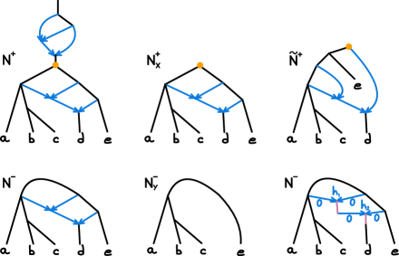
Figure 1: Example rooted network $N^{+}$ on $X=\{a,b,c,d,e\}$; LSA network $N^{+}_{X}$; semidirected network $N^{-}$, subnetwork $N^{-}_{Y}$ on $Y=\{a,b,c,e\}$; network $\tilde{N}^{+}$ obtained by rerooting $N^{-}$ (on one of the hybrid edges); and a display of $N^{-}$ illustrating the modification of edge lengths to zip-up $N^{-}$. Hybrid edges are in blue with arrows. Lowest common ancestor nodes are large (orange) dots.

Definition 2 (semidirected network).

A semidirected graph $G^{-}=(V,E)$ is a tuple where $V$ is the set of nodes, and $E=E_{D}\sqcup E_{U}$ with a set $E_{D}$ of directed edges and a set $E_{U}$ of undirected edges. $E_{D}$ consists of ordered pairs $(a,b)$ where $a,b\in V$. In contrast, $E_{U}$ consists of unordered pairs $\{a,b\}$, such that if $\{a,b\}\in E_{U}$, then $(a,b)\not\in E_{D}$, i.e. an edge cannot be both directed and undirected.

Let $(N^{+},f)$ be a rooted network on $X$. The topological semidirected phylogenetic network induced from $(N^{+},f)$ is a tuple $(N^{-},f)$, where $N^{-}$ is the semidirected graph obtained by:

1. removing all the edges and nodes above $\text{LSA}(X)$;

2. undirecting all tree edges $e\in E_{T}$, but keeping the direction of hybrid edges;

3. suppressing $s=\text{LSA}(X)$ if it has degree $2$: if $s$ is incident to two tree edges, then remove $s$ and replace the two edges with a single tree edge; if $s$ is incident to one tree edge and one hybrid edge, then remove $s$, and replace the two edges by a hybrid edge with the same direction as the original hybrid edge. (Note that $s$ may not be incident to two hybrid edges if it has degree 2 by Lemma 1 in 2019banos ).

For a semidirected graph $M^{-}$ with vertex set $V$ and labelling function $g:X\to V$, $(M^{-},g)$ is a topological semidirected phylogenetic network if it is the semidirected network induced from some rooted network.

Remark.

An alternate definition may consider skipping step 1, that is, retain nodes and edges above the lowest stable ancestor, for a more general class of semi-directed networks. We consider step 1 because the subgraph above the LSA is not identifiable from pairwise distances. Other authors make assumptions that are similar to performing step 1, such as assuming the network is “proper” (every cut-edge and cut-vertex induces a non-trivial split of $X$ francis-moulton-2018 ; fischer18_unroot_non_binar_tree_based_phylog_networ , or “recoverable”, i.e. $\text{LSA}(N)=\rho(N)$ huber14_how_much_infor_is_needed )

For a semidirected network $N^{-}$ induced from $N^{+}$, the sets $V_{L}$, $V_{H}$ and $V_{T}$ are still well defined: $V_{L}(N^{-})=V_{L}(N^{+})$ is the set of nodes with degree 1, thanks to our requirement that leaves must be of degree 1 in a rooted network, and because a root of degree-1 would be above the $\text{LSA}(X)$ in the rooted network. Hybrid nodes $V_{H}(N^{-})=V_{H}(N^{+})$ remain well-defined in a semidirected network, because hybrid edges are directed and point to hybrid nodes. $V_{T}(N^{-})$ is the set of all the other nodes, and may include the original root. The notion of child (node or edge) is also well defined for hybrid nodes in semidirected networks. Indeed, the child edges of a hybrid node are all the incident tree edges and outgoing hybrid edges. Consequently, the notion of tree-child network steel16_phylogeny also carries over.

For a rooted network $N^{+}$ on $X$, the LSA network $N^{+}_{X}$ of $N$ is the rooted network obtained from $N^{+}$ by removing everything above $\text{LSA}(X)$ in $N$ 2019banos . If $N$ has the property that $\rho(N)=\text{LSA}(X)$, then we call $N$ an LSA network. One immediate consequence of these definitions is that the semidirected network induced from $N^{+}$ and $N^{+}_{X}$ are the same. Furthermore, every semidirected network can be induced from an LSA network.

The unrooted graph $U(N)$ induced from a directed or semidirected graph $N$ is the undirected graph obtained from $N$ by undirecting all edges in $N$. Because rooted networks are DAGs, there cannot be directed cycles in rooted or semidirected networks. A cycle in a rooted or semidirected network $N$ is defined to be a subgraph $C$ of $N$, such that $U(C)$ is a cycle.

One may also consider rerooting a semidirected network $N^{-}$: either at a node or on an edge gambette2012_quartets_unrooted . Specifically, rerooting at node $s$ refers to designating a node $s$ in $N^{-}$ as root and directing all undirected (tree) edges away from $s$, if this leads to a valid rooted network. Rerooting on edge $uv$ refers to adding a new node $s$, replacing $uv$ by two edges $us$ and $sv$, and finally rerooting at node $s$. It follows from Definition 2 for semidirected network $N^{-}$ that there exists either a node $u$ or an edge $e$ such that rerooting at $u$ or rerooting on $e$ gives an LSA network $N$ which induces $N^{-}$: we can reroot at $\text{LSA}(X)$ if it is not suppressed, or otherwise reroot at the edge $e$ where $\text{LSA}(X)$ is suppressed. Note that while there is always a rerooting of $N^{-}$ that gives a rooted LSA network, not all rerootings give an LSA network.

Because this work focuses on semidirected networks, in the later sections for notational convenience we will usually denote a semidirected network without the superscript, i.e. $N$ instead of $N^{-}$, and use $N^{+}$ for an LSA network that induces $N$, which is obtained from rerooting at a node or on an edge.

A rooted network is binary if its root has degree $2$ and all the other nodes, except for leaves, have degree $3$. A semidirected network is binary if all its nodes, except for leaves, have degree $3$. The semidirected network induced by a binary rooted network $N^{+}$ is binary. On topological phylogenetic networks, we can further assign edge lengths and hybridization parameters, also called inheritance probabilities, to obtain metric phylogenetic networks.

Definition 3 (metric).

A metric on a rooted or semidirected network $N$ is a pair of functions $(\ell,\gamma)$, with $\ell:E\to\mathbb{R}_{\geq 0}$ assigning lengths to edges, and $\gamma:E_{H}\to(0,1)$ assigning hybridization parameters to hybrid edges. The hybridization parameter $\gamma(e)$ for a hybrid edge $e$ represents the proportion of genetic material that the child inherits through the edge. As a result, we require that for a hybrid node $v$, $\sum_{e\in E_{H}(v)}\gamma(e)=1$, where $E_{H}(v)$ denotes the set of incoming hybrid edges for $v$. We define $\gamma(e)=1$ for any tree edge $e$, to extend the function $\gamma:E\to[0,1]$ to all edges of $N$. A rooted/semidirected network with a metric is called a metric rooted/semidirected network.

In a metric semidirected network, when a node is suppressed (see step 3 in Def. 2), the length of the new edge is the sum of the original two edges. The hybridization parameter is unchanged for hybrid edges.

Two metric and/or semidirected networks are isomorphic if the (semi)directed graphs are isomorphic with an isomorphism that preserves the labelling and the metric. We regard isomorphic networks as identical, as we only identify networks and their properties up to isomorphism.

Definition 4 (blob, level, tree of blobs).

A blob $B$ in a rooted or semidirected network $(N,f)$ is a subgraph of $N$ such that $U(B)$ is a $2$-edge-connected component of $U(N)$. A blob is trivial if it has a single node. The edge-level (or simply level) of a blob $B$ is the number of edges in $B$ one needs to remove in order to obtain a tree (i.e. $\lvert E_{B}\rvert-\lvert V_{B}\rvert+1$, where $E_{B},V_{B}$ are the edge set and node set of the blob $B$). The level of a network is the maximum level of all its blobs. The tree of blobs $\text{BT}(N)$ of a network $N$ is an undirected graph where each vertex is a blob of $N$, and where two vertices $B_{1}$ and $B_{2}$ are adjacent if there is an edge $b_{1}b_{2}$ or $b_{2}b_{1}$ in $N$ such that $b_{1}\in B_{1}$ and $b_{2}\in B_{2}$. The degree of a blob is the degree of the corresponding vertex in the tree of blobs.

Remark.

If $N^{+}$ is an LSA network and $N^{-}$ is induced from it, then $N^{+}$ and $N^{-}$ have the same blobs and the same tree of blobs, because they have the same undirected graphs.

Recall that a graph is $2$-edge-connected if the removal of one edge does not disconnect the graph. A $2$-edge-connected component is a maximal $2$-edge-connected subgraph. Our definition of level follows gambette2012_quartets_unrooted and is nonstandard in using $2$-edge-connected components rather than biconnected components. A graph is biconnected if the removal of one vertex does not disconnect the graph. A biconnected component of a graph, or block, is a maximal biconnected subgraph. Any block of $3$ or more nodes is $2$-edge-connected, so each non-trivial block maps to a single blob and each blob may be formed by one or more block(s). Therefore, the traditional level based on biconnected components is lower than or equal to the level used here. However, the two definitions agree on binary networks. For binary networks, the level of a blob $B$ is the same as the number of hybrid nodes in $B$ gambette2012_quartets_unrooted . If hybrid nodes may have more than two parents, the level of a blob could be greater than its number of hybrid nodes.

The “tree of blobs” was first defined by gusfield07_decom_theor_phylog_networ_incom_charac , using blocks and after modifying the network with edges to separate overlapping blocks. It is easy to verify that non-trivial blocks and blobs are identical after these modifications. Despite the similar name and construction, the tree of blobs is different from the “blob tree” defined in murakami19_recon_tree_child_networ_from .

Unlike blocks, blobs partition the nodes in $N$ and provide a convenient mapping of edges from the tree of blobs to the network, as we will show later. Fig. 2 (left) shows a non-binary network with one blob of level $2$, but with two level-$1$ blocks. There are $3$ ways to refine this network into a binary network, one of which is of level $1$ with $2$ blobs (Fig. 2 right), and the other two are of level $2$ with a single non-trivial blob (and block). Fig. 3 shows a level-$1$ network with $3$ blobs (left) and its tree of blobs (top right). Note that both networks on the top row have the same block-cut tree (derived from blocks and cut nodes, see diestel-graphtheory ) after suppressing its degree-2 nodes, and both networks at the bottom have a block-cut tree reduced to a star, after suppressing degree-2 nodes.

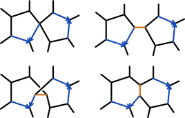
Figure 2: Example networks and their levels. Top left: network $N$ with 1 blob but 2 biconnected components. Hybrid edges are shown in blue with arrows. Top right: one possible resolution of $N$, with identical average distances if the added edge (orange, cut edge) is assigned length 0. It has 2 blobs and is of level 1. Bottom: the other 2 resolutions of $N$, with identical average distances if the added edge (orange) is assigned length 0. Both have $1$ blob and are of level $2$.

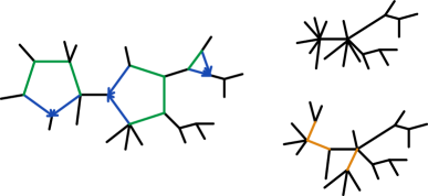
Figure 3: Example tree of blobs. Left: level-1 network $N$, with leaf labels omitted to avoid clutter. Hybrid edges are shown in blue; cut edges in black. The two 5-cycles are identifiable provided that their tree (green) edges have positive length (e.g. Corollary 13). Top right: tree of blobs $T$ for $N$. One of its degree-3 nodes corresponds to a degree-3 blob in $N$, undetectable from average distances. Bottom right: distance split tree reconstructed from average distances. It is a refinement of $T$ (and is $N$’s block-cut tree after suppressing degree-2 nodes). The extra edges (orange) correspond to polytomies in $N$.

2.2 Average distances

Definition 5 (up-down path, rooted network, from Bordewich_2018 ).

In a rooted network $N^{+}$, an up-down path between two nodes $u$ and $v$ is a sequence of distinct nodes $u=u_{1}u_{2}\dots u_{n}=v$ with a special node $s=u_{i}$ such that $u_{i}\dots u_{2}u_{1}$ and $u_{i}\dots u_{n-1}u_{n}$ are directed paths in $N^{+}$.

If $u_{1}u_{2}\dots u_{n}$ is an up-down path, we may write $u\leftarrow s\rightarrow v$ or $u\leftrightarrow v$ as a shorthand. Particularly, a directed path between $u$ and $v$ is also an up-down path, and we will simply write $u\rightarrow v$ or $u\leftarrow v$, depending on the direction of the path. Note that the up-down paths $u_{1}u_{2}\dots u_{n}$ and $u_{n}u_{n-1}\dots u_{1}$ are considered to be the same. Formally, we can define up-down paths as the equivalence classes of these sequence of nodes, with reversal of the sequence being an equivalence relation.

It is not obvious whether the notion of up-down paths is still valid in semidirected networks: given an up-down path $p=u_{0}u_{1}\dots u_{n}$ in a rooted network $N^{+}$, is it possible to tell if $p$ is an up-down path by looking at the induced semidirected network $N^{-}$ alone? It turns out the answer is yes: the notion of an up-down path only has to do with the semidirected structure of a network. An alternative definition that also applies to the semidirected networks is the following:

Definition 6 (up-down path, semidirected network).

Let $N$ be a rooted or semidirected network. An up-down path is a path of distinct nodes with no v-structure. More formally, $u_{0}u_{1}\dots u_{n}$ is an up-down path if the $u_{i}$’s are distinct; for each $i$, either $u_{i}u_{i+1}$ or $u_{i+1}u_{i}$ is an edge in $N$ (for a tree edge $uv$ in semidirected network $N$, both $uv$ and $vu$ are valid edges in $N$); and there is no segment $u_{i-1}u_{i}u_{i+1}$ such that $u_{i}$ is a hybrid node and $u_{i-1}u_{i}$ and $u_{i+1}u_{i}$ are hybrid (directed) edges in $N$. An up-down path with no hybrid nodes is a tree path.

This following equivalence is proved in appendix A.1.

Proposition 1.

Let $N^{+}$ be a rooted network with induced semidirected network $N^{-}$. $p$ is an up-down path in $N^{+}$ according to Definition 5 if and only if it is an up-down path according to Definition 6.

Given a metric $(\ell,\gamma)$ on a network $N$ and a up-down path $p$, we can define the path length $\ell(p)=\sum_{e\in p}\ell(e)$ where $e$ ranges over the edges in path $p$. We also define the path probability $\gamma(p)=\prod_{e\in p}\gamma(e)$ as the product of all the hybridization parameters of the component edges. Here we use the convention of $\gamma(e)=1$ when $e$ is a tree edge. $\gamma(p)$ is the probability of path $p$ being present in a random tree extracted from $N$, where tree “extraction” proceeds as follows: at a hybrid node $h$, we pick one of $h$’s parent hybrid edge according to the edges’ hybridization parameters, and delete all other parent edges of $h$. If we do this independently for all hybrid nodes, then the result is a random tree $T$ with the same nodes as $N$. In $T$, there is a unique path between $u$ and $v$, which equals $p$ with probability exactly $\gamma(p)$.

In the special case that there is a tree path $p$ between nodes $u$ and $v$ in $N$, then we immediately have $\gamma(p)=1$. In fact, $p$ must be the unique up-down path between $u,v$: because $p$ does not contain any hybrid nodes, $p$ is the unique path between $u,v$ on any displayed tree $T$.

Definition 7 (average distance).

Let $N$ be a rooted or semidirected network. The average distance between two nodes $u$ and $v$ in $N$ is defined as

$$d(u,v)=\sum_{p\in P_{uv}}\gamma(p)\ell(p)$$

where $P_{uv}$ denotes the set of up-down paths between $u$ and $v$. Equivalently, this is the expected distance between $u$ and $v$ on a random tree $T$ extracted from $N$ (described above). As a result, $d$ satisfies the triangle inequality. We may write $d_{N}$ to emphasize the dependence on $N$.

The same definition was used for rooted networks by willson12_tree_averag_distan_certain_phylog . By considering our extended definition of up-down paths, our definition clarifies that average distances are well-defined on semidirected networks.

Remark.

In a network $N$, contracting a tree edge of length 0 creates a network $\widetilde{N}$ that has a polytomy, but whose up-down paths are in bijection with those of $N$ and such that $N$ and $\tilde{N}$ have identical average distances. Consequently, a polytomy at a tree node of degree 4 has 3 distinct resolutions with identical average distances. This is not true for hybrid edges of length 0: hybrid edges may not be contracted without modifying the set of up-down paths. Moreover, if there is a polytomy at a hybrid node with 2 incoming hybrid edges and 2 other (outgoing) edges (Fig. 4 left) then there is a single resolution of this polytomy with identical set of up-down paths and identical pairwise distances: with the addition of a tree edge (Fig. 4 center). The resolutions shown in Fig. 4 (right) are not equivalent: there exist up-down paths $a\rightarrow c$, $a\rightarrow d$, $b\rightarrow c$ and $b\rightarrow d$ in the network on the left, but each network on the right is missing one of these paths.

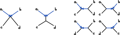
Figure 4: A polytomy below a hybrid node (left) can be resolved by adding a new edge of length $0$. The only resolution with identical up-down path lengths and average distances is by adding a new tree edge (middle). Contracting the horizontal hybrid edge in any network on the right to match the topology on the left would affect up-down paths and average distances.

Definition 8 (subnetwork, from 2019banos ).

Let $N^{-}$ be a semidirected network on $X$, and $Y\subset X$. Then the induced network $N_{Y}^{-}$ on $Y$ is obtained by taking the union of all up-down paths in $N^{-}$ between pairs of tips in $Y$.

If $N^{+}$ is a rooted version of $N^{-}$, then it is possible to reroot $N_{Y}^{-}$ at $\text{LSA}(Y)$ in $N^{+}$, which belongs in $N_{Y}^{-}$ as shown in 2019banos . $N_{Y}^{-}$ naturally inherits the metric from $N^{-}$: the distance between any pair of taxa $x,y\in Y$ is the same in $N_{Y}^{-}$ and in $N^{-}$ because the up-down paths between $x,y$ are preserved, together with the edge lengths and hybridization parameters on these paths.

2.3 Main results

Since distances are defined on up-down paths, and up-down paths are identical on a rooted network and its induced semidirected network, it follows from Proposition 1 that average distances are independent of the root location on a rooted network, so that the root is not identifiable from average distances:

Proposition 2.

If rooted networks $N_{1}^{+}$ and $N_{2}^{+}$ induce the same semidirected network $N^{-}$, then pairwise distances on $N_{1}^{+}$ and $N_{2}^{+}$ are identical.

What may be identifiable from average distances, at best, is the semidirected network $N^{-}$ induced from $N^{+}$, unless further assumptions are made.

Several papers have considered average distances on networks before, with different assumptions on the networks. willson13_recon_certain_phylog_networ_from worked with binary networks and assumed the knowledge of the root, that is, the root was one of the labelled leaves and pairwise distance data was given between the root and the other leaves. francis-steel-2015 also worked with binary networks and assumed that hybrid edges have length $0$, along with other assumptions.

The remainder of the work focuses on the following problem: Given the average distances between tips, what can we identify about the semidirected network: what topological structures, and what continuous parameters?

2.3.1 Non-identifiable features

We first cover negative results, on features that are not identifiable from average distances. The simplest such feature is the “hybrid zipper” (Fig. 5). We will show that a network is not distinguishable from its zipped-up version defined below.

Definition 9 (zipped-up network).

In a network, a hybrid node is zipped up if all its parent edges have length $0$. A network is zipped up if all its hybrid nodes are zipped up. If a hybrid node $h$ is not zipped up in a network $N$, the version of $N$ zipped up at $h$ is the network obtained by modifying the edges adjacent to $h$ as follows (we refer to this operation as a zipping-up):

1. If $h$ has $k\geq 2$ children $c_{1},\ldots,c_{k}$ and is not zipped up, add a tree node $w$ and insert a tree edge $hw$ of length $0$ as unique child edge of $h$, then delete each edge $hc_{i}$ and replace by $wc_{i}$ with identical length (see Fig. 5).

2. Set the length of the unique child edge $hw$ of $h$ to

   $$l_{h}=\ell(hw)+\sum_{u\text{\,parent of\,}h}\gamma(uh)\ell(uh)$$ (1)

   then set the length of all its parent hybrid edges to $0$.

The zipped-up version of a network $N$ is the network obtained by zipping-up $N$ at all its unzipped hybrid nodes repeatedly.

In appendix A.2, we prove that the zipped-up version is unique. Note that a hybrid node may need to be zipped multiple times before the network is fully zipped up. In network $N^{-}$ from Fig. 1 (bottom right) for example, $h_{2}$ may need to be zipped-up twice if it is considered before $h_{1}$.

Figure 5: Zipping up: network transformation of branch lengths, setting hybrid edge lengths to $0$. The new length $l_{h}$ is given in (1). In case of a polytomy below the hybrid node (right), a new tree edge of length $0$ needs to be added before zipping up.

Proposition 3 (hybrid zip-up).

Let $N$ be a semidirected network, $h$ be a hybrid node in $N$ with parents $u_{1},\dots,u_{n}$. If $h$ has more than one child, then step 1 in Definition 9 does not affect average distances. If $h$ has one child $w$, then the average distances between the tips depend on $\ell(u_{1}h),\ldots,\ell(u_{n}h),\ell(hw)$ only through $l_{h}$ given by (1). Therefore, zipping up $N$ at $h$ does not change average distances.

The proof is in section 3.1. This unidentifiability problem was mentioned in Pardi_2015 , where it is referred to as “unzipping”, as well as in willson13_recon_certain_phylog_networ_from . It is important to note that because we use average distances instead of displayed trees in Pardi_2015 , we have an extra degree of freedom: As in unzipping, we can subtract an equal amount $\epsilon$ in lengths from both $uh$ and $vh$, and add $\epsilon$ to $hw$. This leaves the average distances unchanged. What is new with average distances is that we can also “slide” the hybrid node along the v-structure, that is: subtract $(1-\gamma)\epsilon$ from $uh$ and add $\gamma\epsilon$ to $vh$. This has no impact on the average distances either.

Because of the extra degree of freedom, instead of “fully unzipping” each reticulation as in Pardi_2015 and working with networks where outgoing edges from hybrid nodes have length $0$, we shall restrict our attention to zipped-up networks, which are networks where all the hybrid edges have length $0$ (defined rigorously below). This requirement is also present in willson12_tree_averag_distan_certain_phylog and willson13_recon_certain_phylog_networ_from , but the non-identifiability underlying this requirement was not clarified. The requirement was motivated by the fact that hybridizing populations must be contemporary with each other. However, hybrid edges of positive length appear naturally when hybridizations involve “ghost” populations that went extinct or with no sampled descendants, or when two populations fuse, such as if their habitat becomes less fragmented degnan2018 .

Proposition 4 (shrinking blobs of degree 2 or 3).

Let $B$ be a blob of degree 2 or 3 in a semidirected network $N$. Then $N^{\prime}$, the network obtained by shrinking $B$ (i.e. identifying the nodes in $\partial B$ and deleting the other nodes in $B$) and modifying the lengths of the cut edges adjacent to $B$, induces the same pairwise distances.

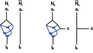
Figure 6: Any blob of degree $2$ (left) or $3$ (right) can be shrunk while preserving average distances.

Section 3.2 presents a more general Lemma 15 to swap a subgraph with another within a semidirected network while keeping the average distances, from which Proposition 4 follows as a corollary. Proposition 4 is used in many proofs when considering subnetworks. If a blob reduces to a degree-2 or degree-3 blobs after subsampling leaves, then it can be ignored, up to the lengths assigned to the edges replacing the blob. A consequence of Proposition 4 is that we require networks to not have degree-2 or degree-3 blobs in many of our results. Equivalently, this requirement can be interpreted as considering networks after these blobs have been shrunk and edge lengths modified appropriately. Parallel edges may form a degree-2 blob. Even if they are part of a larger blob, they can be swapped with a single tree edge:

Proposition 5 (merging parallel edges).

In a network $N$, let $h$ be a hybrid node such that all its parent edges $e_{1},\dots,e_{n}$ are incident to the same nodes, $v$ and $h$. Consider the network $N^{\prime}$ obtained by replacing $e_{1},\dots,e_{n}$ by a single tree edge $e=(vh)$ of length $\sum_{i}\gamma(e_{i})\ell(e_{i})$. Then $d_{N}=d_{N^{\prime}}$.

This proposition, proved in section 3.2, gives a rationale for a traditional assumption that rooted phylogenetic networks do not have parallel edges steel16_phylogeny , despite the biological realism of parallel edges. First, parallel edges can arise from extinction or unsampled taxa: hybridization between distant species would appear as a pair of parallel edges if all the descendants of the two parental species are extinct or not sampled. Second, a species may split into 2 populations and then merge back into a single population due to evolving geographic barriers, such as glaciations. Therefore, we allowed for parallel edges in our network definition. Also, parallel edges may be identifiable from models and data other than average distances degnan2018 .

Similarly, $3$-cycles are not identifiable: any $3$-cycle (which may be part of a larger blob) can be shrunk to a single node with the loss of one reticulation, without affecting average distances (Fig. 7).

Figure 7: Any $3$-cycle can be swapped while preserving average distances. (a) A 3-cycle with a single reticulation (left) can be swapped by a subgraph without reticulation (right). (b) A 3-cycle with 2 reticulations (left) can be swapped by a single reticulation (right). See Proposition 6 for edge length adjustments. (c) A ladder of reticulations between sister lineages (left) can be eliminated (right) by repeated swaps.

Proposition 6.

Let $N$ be a semidirected network on $X$, $h$ a hybrid node in $N$ with exactly two parents $u$ and $v$. Let $\gamma_{1}=\gamma(uh)$ and $\gamma_{2}=\gamma(vh)=1-\gamma_{1}$.

1. If $uv$ is a tree edge (Fig. 7a), then let $N^{\prime}$ be the semidirected graph obtained by shrinking the 3-cycle $u,v,h$ as follows: remove edges $uh$, $vh$, and $uv$; add tree node $w$; add tree edges $uw$, $vw$, and $wh$ with lengths

   $$\ell(uw)=\gamma_{2}\ell(uv),\quad\ell(vw)=\gamma_{1}\ell(uv),\quad\ell(wh)=\gamma_{1}\ell(uh)+\gamma_{2}\ell(vh)\,.$$

2. If $uv$ is a hybrid edge (Fig. 7b) and if $v$ has exactly two parents $u$ and $x$ that are not adjacent, then let $\gamma_{3}=\gamma(uv)$ and let $N^{\prime}$ be the semidirected graph obtained by shrinking the 3-cycle as follows: remove $uv$; make the other parent edge of $v$ a tree edge; and set

   $$\gamma(uh) =\gamma_{1}+\gamma_{2}\gamma_{3}\;\mathchar 24635\relax\;\quad\gamma(vh)=\gamma_{2}(1-\gamma_{3})$$

   $$\ell(uh) =\big{(}\gamma_{2}\gamma_{3}(\ell(uv)+\ell(vh))+\gamma_{1}\ell(uh)\big{)}/(\gamma_{2}\gamma_{3}+\gamma_{1})\,.$$

Then $N^{\prime}$ is a semidirected network on $X$ with one fewer reticulation than $N$, and $N^{\prime}$ induces the same average distances as $N$ on $X$. We may also suppress the degree-$2$ nodes in $N^{\prime}$, which does not affect pairwise distances.

Proposition 6 also follows from the swap lemma and is proved in section 3.2. Note that in case 2, if $u$ and $x$ are adjacent, then we may first shrink the 3-cycle $xvu$ before proceeding and shrinking $uvh$, possibly recursively (Fig. 7c). The lack of identifiability of 3-cycles and blobs of degree 2 or 3 explains the special cases found by francis-steel-2015 when characterizing networks whose average distances fit on a tree. For some classes, these networks must be trees except for some local non-tree-like structures. Namely, the class of “primitive 1-hybridization” networks was defined to allow for a short cycle near the root. When the root is suppressed, this cycle becomes a 3-cycle. Also, distances from “HGT networks” may fit a tree despite a series of gene exchange between sister species (Fig. 7c), which form a degree-3 blob. Our general characterization explains why these local structures are invisible from average distances, found by francis-steel-2015 .

The hybrid zippers and $3$-cycles are not the end of identifiability problems. Here we give an example of a level-2 network that is not identifiable (with generic parameters), showing that in general, it is not possible to identify the topology of a network with average distances, even when requiring no degree-2 or 3 blobs and zipped-up reticulations. As a result, with average distances, we can only aim to identify networks given restrictions, or identify only certain features of networks.

Theorem 7.

Let $k\geq 2$. Consider the space $\cal S$ of zipped-up binary semidirected networks of level at most $k$ on $n\geq 4$ taxa, with no $2$- or $3$-cycles. Networks in $\cal S$ are not generically identifiable from average pairwise distances, in the sense that there exists network topologies $N_{1}\neq N_{2}$ in $\cal S$ and sets of parameters $\Omega_{1}$ and $\Omega_{2}$ with positive Lesbegue measure satisfying the following: for any $(\ell_{1},\gamma_{1})\in\Omega_{1}$, there exists $(\ell_{2},\gamma_{2})\in\Omega_{2}$ such that the average distances defined by $(N_{1},\ell_{1},\gamma_{1})$ and $(N_{2},\ell_{2},\gamma_{2})$ are identical.

The proof is presented in section 5.1. In short, the main idea is to find examples on $4$ taxa, and then embed these examples in larger networks for any $n$. Fig. 8 provides examples of topologies that can serve the role of $N_{1}$ and $N_{2}$ in Theorem 7 for $n=4$. The network on the left is of level 1, showing that level-2 networks are not distinguishable from level-1 networks in general. Also, the network on the right is tree-child, implying that Theorem 7 also holds for the smaller class of tree-child networks of level at most $k$ (zipped and without any 2- or 3-cycles), thus providing a stronger statement.

Figure 8: Semidirected networks with identical average distances on a parameter set of positive Lebesgue measure. The network on the right is tree-child.

2.3.2 Identifiable features

Now we move on to positive results, i.e. what we can identify of a network from average distances, subject to certain constraints.

Theorem 8 (identifying the tree of blobs).

For a semidirected network $N$ with no degree-2 blob and no internal cut edge of length $0$, a refinement of the tree of blobs can be constructed from pairwise average distances, and which we call the distance split tree.

Theorem 8 is proved in section 4. The distance split tree is defined rigorously in section 4, Definition 12. Its construction is based on average distances alone.

Next, we provide examples showing that the tree of blobs cannot be reconstructed without further assumptions, and that the restriction of reconstructing a refinement is necessary. A refinement of tree $T$ is a tree $T^{\prime}$ such that we can obtain $T$ by contracting edges of $T^{\prime}$.

Example 1.

Consider the network $N$ in Fig. 9 (left). Let $t_{i}$ and $\gamma_{i}$ denote edge $i$’s length and hybridization parameter. $N$ is a binary network of level 2. Its tree of blobs is a star (Fig. 9 center). Its average distances are equal to those obtained from a tree (Fig. 9 right) for specific parameter values, namely when $\gamma_{3}=t_{2}/(t_{1}+t_{2})$ and $\gamma_{7}$ is small enough, and the same topology is obtained by the distance split tree from Theorem 8. In this case, the distance split tree is a strict refinement of the tree of blobs $\text{BT}(N)$, but is an exact and parsimonious explanation of the distances. We also note that under generic parameters, the distance split tree is equal to the star tree of blobs (see section 4 for the proofs).

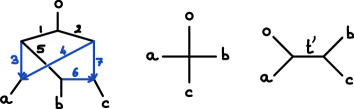
Figure 9: Example of a binary network $N$ of level 2 (left) whose tree of blobs is a star (middle). The distance split tree $T$ is also a star for generic parameters. But if $\gamma_{3}=t_{2}/(t_{1}+t_{2})$ and $\gamma_{7}$ is small, then $T$ is a strict refinement of the tree of blobs (right). In this case, $N$ and $T$ have identical average distances.

Example 2.

Consider the networks $N_{1}$ and $N_{2}$ in Fig. 10. $N_{1}$ is not binary. It has one blob, made of two biconnected components, and its tree of blobs is a star. $N_{2}$ is a binary resolution of $N_{1}$ with two blobs: one for each block of $N_{1}$. Since the extra cut-edge in $N_{2}$ has length 0, $N_{1}$ and $N_{2}$ have the same average distances and the same distance split tree $T$ (Fig. 10 right). $T$ is a strict refinement of $N_{1}$’s tree of blobs, but it is the tree of blobs of $N_{2}$: it recovers the separate blocks with the extra cut edge. In this case again, the distance split tree represents a true feature of the network.

These examples and our results on non-binary level-1 networks (below) lead us to state the following conjecture.

Conjecture 9 (distance split tree as tree of blobs of equivalent network).

Let $N$ be a metric semidirected network on taxon set $X$, $d_{N}$ its average distances on $X$, and let $T$ be the distance split tree reconstructed from $d_{N}$. Then there exists a semidirected $N^{\prime}$ of level equal or less than that of $N$ with $d_{N^{\prime}}=d_{N}$ and such that $T$ is the tree of blobs of $N^{\prime}$.

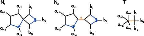
Figure 10: Left: example of a non-binary level-2 network $N_{1}$. Middle: $N_{2}$ is one possible resolution of $N_{1}$. $N_{2}$ is of level 1, with an extra cut edge of length $0$ (in orange). Right: tree of blobs $T$ of $N_{2}$. If, for example, $\ell(e)=1$ for all edges in $N_{1}$ and $\gamma(e)=0.5$ for all hybrid edges, then the distance split tree for $N_{1}$ is $T$, which is a strict refinement of $N_{1}$’s tree of blobs (a star). Note that the other resolutions of $N_{1}$ have a star as their tree of blobs.

In Theorem 10 below (proved in section 4), we add assumptions to identify the tree of blobs exactly. When we limit the network to be of level 1, we characterize the distance split tree exactly: it is the tree of blobs refined by extra edges to partially resolve polytomies adjacent to blobs.

Theorem 10.

Let $N$ be a level-$1$ network with internal tree edges of positive length and with no degree-$2$ blob. Then the distance split tree of $N$ is the tree of blobs of $N^{R}$, where $N^{R}$ is the network obtained as follows. For each non-trivial blob $B$ in $N$ and each node $u$ in $B$, let $\{a_{1}u,\ldots,a_{k}u\}$ be the set of edges of $u$ that are not in $B$. If $k\geq 2$, then refine the polytomy at $u$ by creating a new node $u^{\prime}$, adding tree edge $uu^{\prime}$ of length $0$; and disconnecting each $a_{i}$ from $u$ and connecting it to $u^{\prime}$. That is, for each $i=1,\dots,k$, remove $a_{i}u$ and create tree edge $a_{i}u^{\prime}$.

Remark.

The assumption that internal tree edges have positive length is a weak requirement, because a tree edge of length $0$ can be contracted to create a polytomy.

In the proof, we show that $N^{R}$ is indeed a valid semidirected network, with identical average distances as $N$. The distance split tree from $N^{R}$ is in fact the block-cut tree of $N$ (see “block-cutpoint trees” (harary1971graph, , p.36)), after suppressing its degree-2 nodes. For example, the network in Fig. 3 (left) has a distance split tree with $2$ extra edges (in orange, bottom right) compared to its tree of blobs (top right). If we further assume that the network is binary, then $N=N^{R}$ and the distance split tree equals the tree of blobs:

Corollary 11.

For a binary level-1 semidirected network with internal tree edges of positive length and no degree-2 blob, the tree of blobs can be constructed from average distances.

In a binary level-$1$ network, each blob is a cycle and we can isolate a blob by sampling an appropriate subset of tips. On this subset, the induced subnetwork, after removing degree-$2$ blobs, is a “sunlet” gross18_distin_phylog_networ , that is, a semidirected network with a single cycle and a single pendant edge attached to each node in the cycle. In section 5, we tackle the identifiability of sunlets. Some of these results are special cases of those in willson13_recon_certain_phylog_networ_from (with a simpler proof strategy). One exception is the case of $4$-sunlets, which is excluded by the assumptions in willson13_recon_certain_phylog_networ_from : In general, the $4$-sunlet and its metric $(\ell,\gamma)$ are not identifiable, but the unrooted $4$-sunlet is a structure that can be detected in the tree of blobs.

In section 5, we can characterize all the $4$-sunlets (and their parameters) that give rise to a given average distance matrix. Ideally one would choose a “canonical” $4$-sunlet as the representative of all these distance-equivalent sunlets. However, we did not find a single sensible choice for such canonical $4$-sunlet. Consequently we opt to use a separate split-network type of representation for these $4$-sunlets.

Section 6 introduces mixed networks, in which some parts are semidirected and 4-cycles are undirected. In short, a mixed network encodes the reticulation node and edges in $k$-cycles for $k\geq 5$, and the unrooted topology in 4-cycles, without identification of the exact placement of the hybrid node in a 4-cycle. In section 6, we define this representation rigorously and combine results from sections 4 and 5 to prove the following main result.

Theorem 12 (identifiability of mixed network representation for level-$1$ networks).

Let $N_{1}$ and $N_{2}$ be level-$1$ semidirected networks on $X$ with no $2$ or $3$-cycles or degree-$2$ nodes, and with internal tree edges of positive lengths. Let $N_{i}^{*}$ be the mixed network representation of $N_{i}$ after zipping up its reticulations for $i=1,2$. Then $d_{N_{1}}=d_{N_{2}}$ implies that $N_{1}^{*}=N_{2}^{*}$.

Note that for a network $N$ satisfying the conditions above and its mixed network representation $N^{*}$, $N$ and $N^{*}$ have the same unrooted topology, except that polytomies adjacent to $4$-cycles in $N$ may be partially resolved in $N^{*}$. If we consider the space of level-1 networks with no 4-cycles, we obtain the following result as a special case.

Corollary 13 (identifiability of zipped-up version of level-1 networks).

Let $N_{1}$ and $N_{2}$ be zipped-up level-$1$ semidirected networks on $X$ with tree edges of positive lengths, without any $2$, $3$ or $4$-cycles, and without degree-$2$ nodes. If $d_{N_{1}}=d_{N_{2}}$ then $N_{1}=N_{2}$.

2.4 Biological relevance

In practice, average distances between pairs of taxa need to be estimated from data. allman2022-identifiability-logdet-net studied the identifiability of the network topology using the log-det distance, for level-1 networks and under a coalescent model. Future work could study identifiability of the network and its parameters under various models and for various methods to estimate evolutionary distances, such as the average coalescence time between pairs of taxa liu2009_STAR_STEAC , average internode distance liu2011_NJst , or the $f_{2}$ statistic when many genomes are available from each species peter2016 .

The most frequent reticulations are expected between incipient species, or sister species that just split from each other and have yet to achieve reproductive isolation. Our work shows that these most frequent reticulations are not identifiable from average distances. Only the less frequent events between more distant species can be detected using average distances.

Our work also shows a strong effect of taxon sampling, as observed with real data conover2019_malvaceae ; karimi2020_baobab . Dense taxon sampling is critical to avoid blobs of degree 2 or 3. For example, if a hybridization forms a cycle of degree 5 in a full level-1 network, then it is necessary to sample at least one taxon from across each of the 5 cut edges adjacent to the cycle, for the reticulation to be identifiable from average distances. Conversely, it may be useful to reduce taxon sampling strategically. Reducing the degree of some blobs to be 3 or less in the subnetwork could be a strategy to obtain a more resolved tree of blobs on the reduced taxon set. When the true network is of level greater than 1, different taxon subsamples may lead to different trees of blobs, and to the detection of different reticulation events by methods that assume a level-1 network. While this sensitivity to taxon sampling may be disconcerting, subsampling can decrease the level and bring strength to methods that require low-level networks like SNaQ Sol_s_Lemus_2016_infer and NANUQ Allman_2019 .

Pairwise distances are not unique in causing some features to lack identifiability. From quartet concordance factors for example, some 3-cycles cannot be identified, and the hybrid node position is not always identifiable in a 4-cycle Sol_s_Lemus_2016 ; 2019banos ; solislemus2020_identifiability . Software for network inference should provide information on the class of equivalent networks with identical optimal likelihood, e.g. list the multiple ways to place the reticulation in a 4-cycle. Bayesian approaches could report on sets of networks that cannot be distinguished from the data, and whose relative posterior probabilities are solely influenced by the prior. Interactive visualization tools could facilitate the exploration of networks with equivalent scores, so practitioners could avoid interpretations that hinge on a strict subset of these networks. If software is misleadingly presenting a single network as being optimal without presenting the whole class of networks with equivalent fit, then undue confidence could be placed on some interpretation.

3 Proofs related to non-identifiable features

3.1 Hybrid zip-up

To prove Proposition 3, we first need the following definition and proposition.

Definition 10 (displayed tree).

Let $N$ be a directed or semidirected network. For hybrid node $h$, let $E_{H}(h)$ be its parent hybrid edges. Let $T$ be the graph obtained by keeping one hybrid edge $e\in E_{H}(h)$ and deleting the remaining edges in $E_{H}(h)$, for each hybrid node $h$ in $N$. Then $T$ is a tree, and is called a displayed tree. The distribution on displayed trees generated by $N$ is the distribution obtained by keeping $e\in E_{H}(h)$ with probability $\gamma(e)$, independently across $h$.

Note that $T$ is a tree because it is a DAG (considering $N$ as rooted), all the nodes are still reachable from the root, and all nodes have in-degree at most $1$.

Proposition 14.

Let $N$ be a (directed or semidirected) network. For two nodes $u$ and $v$ and tree $T$, let $q_{uv}(T)$ be the unique path between $u$ and $v$ in $T$. Then, for a given up-down path $p$ between $u$ and $v$ in $N$,

$$\mathbb{P}(q_{uv}(T)=p)=\gamma(p)$$

where the probability is taken over a random tree $T$ displayed in $N$. As a result,

$$d(u,v)=\mathbb{E}\ell(q_{uv}(T))$$

where $d(u,v)$ is the distance between $u,v$, and $\ell(q)$ is the length of path $q$.

Proof: Since rooting a semidirected network does not change the process of generating displayed trees, nor up-down paths in the network, it suffices to consider the case when $N$ is a directed network. Let $p$ be an up-down path in $N$. Let $E=\{e_{1},\dots,e_{n}\}$ be the set of hybrid edges in $p$, and let $H=\{h_{1},\dots,h_{n}\}$ where $h_{i}$ is the child of $e_{i}$. All the $h_{i}$’s are distinct hybrid nodes because the up-down path $p$ may not go through partner hybrid edges (no v-structure). It suffices to show that $p=q_{uv}(T)$ if and only if for each $h_{i}\in H$, $e_{i}$ is kept.

The “only if” part is evident since $e_{i}$ has to be in $T$ for $p$ to be in $T$. Now consider a displayed tree $S$ where for all $h_{i}\in H$, $e_{i}$ is kept. Because all of the edges of $p$ are in $S$, $p$ is a path between $u$ and $v$ in $S$; and since $S$ is a tree, $p$ is the unique path between $u$ and $v$ in $S$.

Proof: [Proof of Proposition 3 (hybrid zip-up)] If $h$ has more than one child, then step 1 in Definition 9 does not modify the set of up-down paths, other than inserting $hw$ to the paths containing $u_{i}h,hc_{j}$ for some parent $u_{i}$ and child $c_{j}$ of $h$. Since the length of $hw$ is set to 0, step 1 does not change the length of up-down paths, nor average distances. If $h$ has a single child $w$, we first assume that $h$ is the only hybrid node in $N$. Let $a_{i}=\ell(u_{i}h)$ and $\gamma_{i}=\gamma(u_{i}h)$ for $i=1,\dots,n$ and let $t=\ell(hw)$. Let $x,y$ be two tips of $N$. There are two cases:

1. If some up-down path $p$ between $x,y$ does not contain $h$, then $p$ must be the unique up-down path between $x$ and $y$. This is because $p$ is a path on the $n$ displayed trees of $N$. Consequently the distance between $x$ and $y$ does not depend on $a_{1},\ldots,a_{n}$ or $t$, and the statement is vacuously true.

2. If all up-down paths between $x,y$ contain $h$, then there are exactly $n$ up-down paths $q_{i}$, with $q_{i}$ containing the edge $u_{i}h$. In this case the average distance is

   $$d(x,y)=\sum_{i=1}^{n}\gamma_{i}(a_{i}+l_{i}+t)=l_{h}+\sum_{i=1}^{n}\gamma_{i}l_{i},$$

   where $l_{i}=\sum_{e\in q_{i},e\notin\{u_{1}h,\ldots,u_{n}h,hw\}}\ell(e)$ does not depend on $(a_{1},\dots,a_{n},t)$.

For the general case, we use Proposition 14. Let $T$ be a random displayed tree in $N$ and $D_{xy}=D_{xy}(T)$ be the distance between $x$ and $y$ in $T$ (a random quantity). Let $R$ be the set of hybrid edges kept in $T$ at all hybrid nodes except for $h$. By conditioning on $R$, we reduce the problem to a network with a single reticulation: $\mathbb{E}[D_{xy}\mid R]$ is the average distance on a (random) network with a single reticulation at $h$. By the above argument, $\mathbb{E}[D_{xy}\mid R]$ only depend on $(a_{1},\dots,a_{n},t)$ through $l_{h}$. Taking expectation again gives the result.

3.2 Swap lemma and related results

In this section we present a general swap lemma and apply it to prove the non-identifiability of specific features. We first introduce some necessary definitions and notations.

Let $A$ be a subgraph of a semidirected network $N$ on $X$. $A$ is hybrid closed if for any hybrid edge in $A$, all of its partner edges are in $A$. We use $\partial A$ to denote the boundary of $A$ in $N$, defined as the set of nodes in $A$ that are either leaves, or are incident to an edge not in $A$. For two nodes $a,b\in\partial A$, we define

$$\gamma_{A}(a,b)=\sum_{p:\;a\leftrightarrow b\text{ in }A}\gamma(p),$$

where $p$ ranges over the set of up-down paths from $a$ to $b$ that lie entirely in $A$. Then we define the conditional distance in $A$ as

$$d(a,b\mid A)=\begin{cases}\displaystyle\frac{1}{\gamma_{A}(a,b)}\;\sum_{p:\;a\leftrightarrow b\text{ in }A}\gamma(p)\ell(p)&\text{if }\gamma_{A}(a,b)>0\\ 0&\text{if }\gamma_{A}(a,b)=0\end{cases}$$

where in the sum $p$ again ranges over up-down paths between $a,b$ that lie in $A$. The following lemma says that average distances are unchanged if we swap $A$ with another subgraph of identical boundary, provided that $\gamma_{A}$ and $d(.,.\mid A)$ are preserved on $\partial A$.

Lemma 15 (subgraph swap).

Let $N_{1}$ and $N_{2}$ be metric semidirected networks on the same leaf set $X$, with node sets $V(N_{i})=V_{A_{i}}\sqcup V_{B}$ and edge set $E(N_{i})=E_{A_{i}}\sqcup E_{B}$ for $i=1,2$, such that $A_{1}$ and $A_{2}$ are hybrid-closed subgraphs with identical boundary in $N_{1}$ and $N_{2}$ respectively: $\partial A_{1}=\partial A_{2}$, denoted as $\partial A$. If $\gamma_{A_{1}}(a,b)=\gamma_{A_{2}}(a,b)$ and $d_{N_{1}}(a,b\mid A_{1})=d_{N_{2}}(a,b\mid A_{2})$ for every $a,b\in\partial A$, then $d_{N_{1}}=d_{N_{2}}$ on $X$.

Proof: Given an up-down path $p$ and two nodes $a,b$ on the path, we write $a\overset{p}{\longleftrightarrow}b$ for the segment of $p$ between $a,b$, which is an up-down path as well.

We first prove the lemma when there are no hybrid edges in $E_{B}$. For now we consider the distances in $N_{1}$. To simplify notations, we shall write $N=N_{1}$ and $A=A_{1}$. Let $x,y\in X$ be two tips, and $p$ an up-down path between them. Then $p$ can be subdivided into segments that consists of consecutive edges in $E_{B}$, and segments of consecutive edges in $E_{A}$, the set of edges in $A$. Traversing $p$ from $x$ to $y$, let the $j$th segment in $E_{A}$ be $a_{j}\overset{p}{\longleftrightarrow}a_{j}^{\prime}$, where $a_{j},a_{j}^{\prime}\in\partial A$. Note $a_{1}=x$ and $a_{k}^{\prime}=y$ are possible for some $k$, if $x$ or $y$ is in $A$. Given a $2k$-tuple $\bm{a}=(a_{1},a_{1}^{\prime},\dots,a_{k},a_{k}^{\prime})\in\partial A^{2k}$, let $\mathcal{P}_{k}(\bm{a})$ denote the set of up-down paths $p$ between $x$ and $y$ with exactly $k$ segments in $A$, and such that segment $j$ enters and exits $A$ at $a_{j},a_{j}^{\prime}$: $a_{j}\overset{p}{\longleftrightarrow}a_{j}^{\prime}$. The set of up-down paths between $x$ and $y$ can then be written as

$$\bigsqcup_{k\geq 0}\bigsqcup_{\bm{a}\in\partial A^{2k}}\mathcal{P}_{k}(\bm{a}).$$

Consequently, we have

$$d(x,y)=\sum_{k\geq 0}\sum_{\bm{a}\in\partial A^{2k}}\sum_{p\in\mathcal{P}_{k}(\bm{a})}\gamma(p)\ell(p)$$ (2)

For a given $\bm{a}\in\partial A^{2k}$ and $p\in\mathcal{P}_{k}(\bm{a})$, consider the segments in $E_{B}$, which are the segments $a_{j}^{\prime}\overset{p}{\longleftrightarrow}a_{j+1},j=1,\dots,k-1$ and possibly also $x\overset{p}{\longleftrightarrow}a_{1}$ or $a_{k}^{\prime}\overset{p}{\longleftrightarrow}y$ when $x$ or $y$ is in $V_{B}$. These segments are uniquely determined by $k$ and $\bm{a}$ because we assumed no hybrid edges in $E_{B}$. There are no undirected cycles in the subgraph formed by nodes $V_{B}\cup\partial A$ and edges $E_{B}$, so for a given $a_{j}^{\prime},a_{j+1}\in\partial A$, there is either no path or a single (tree) path $a_{j}^{\prime}\leftrightarrow a_{j+1}$ in $E_{B}$. Let $E_{B}(k,\bm{a})$ be the set of edges $e\in E_{B}$ such that $e\in p$ for any (and every) $p\in\mathcal{P}_{k}(\bm{a})$.

The segments of an up-down paths must be up-down paths. Conversely, the concatenation of contiguous up-down paths alternating from $E_{A}$ and $E_{B}$ is still an up-down path, because $E_{B}$ contains tree edges only. Therefore, if $E_{B}(k,\bm{a})$ is non-empty or not needed ($k=1$ and $x,y\in\partial A$), then $\mathcal{P}_{k}(\bm{a})$ is non-empty and there is a bijection between $\mathcal{P}_{k}(\bm{a})$ and $\prod_{j=1}^{k}\mathcal{P}_{1}((a_{j},a_{j}^{\prime}))$: each $p\in\mathcal{P}_{k}(a)$ is mapped to the segments in $E_{A}$, with interleaving segments $E_{B}(k,\bm{a})$. Consequently, if $\mathcal{P}_{k}(\bm{a})$ is not empty then we have

$$\sum_{p\in\mathcal{P}_{k}(\bm{a})}\gamma(p) = \sum_{p\in\mathcal{P}_{k}(\bm{a})}\prod_{i=1}^{k}\gamma(a_{i}\overset{p}{\longleftrightarrow}a_{i}^{\prime})=\sum_{p_{1}\in\mathcal{P}(a_{1},a_{1}^{\prime})}\dots\sum_{p_{k}\in\mathcal{P}(a_{k},a_{k}^{\prime})}\prod_{i=1}^{k}\gamma(p_{i})$$

$$= \prod_{i=1}^{k}\gamma_{A}(a_{i},a_{i}^{\prime})\;.$$

For the first summation in (2), we may then write

$$\sum_{p\in\mathcal{P}_{k}(\bm{a})}\gamma(p)\ell(p) = \!\!\sum_{p\in\mathcal{P}_{k}(\bm{a})}\left(\prod_{i=1}^{k}\gamma(a_{i}\overset{p}{\longleftrightarrow}a_{i}^{\prime})\right)\left(\sum_{e\in E_{B}(k,\bm{a})}\ell(e)+\sum_{i=1}^{k}\ell(a_{i}\overset{p}{\longleftrightarrow}a_{i}^{\prime})\right)$$ (3)

$$= \prod_{i=1}^{k}\gamma_{A}(a_{i},a_{i}^{\prime})\left(\sum_{e\in E_{B}(k,\bm{a})}\ell(e)\right)+$$

$$\sum_{p\in\mathcal{P}_{k}(\bm{a})}\sum_{i=1}^{k}\left(\prod_{j\neq i}\gamma(a_{j}\overset{p}{\longleftrightarrow}a_{j}^{\prime})\right)\gamma(a_{i}\overset{p}{\longleftrightarrow}a_{i}^{\prime})\ell(a_{i}\overset{p}{\longleftrightarrow}a_{i}^{\prime})$$

$$= \prod_{i=1}^{k}\gamma_{A}(a_{i},a_{i}^{\prime})\left(\sum_{e\in E_{B}(k,\bm{a})}\ell(e)\right)+\sum_{i=1}^{k}d(a_{i},a_{i}^{\prime}\mid A)\prod_{i=1}^{k}\gamma_{A}(a_{i},a_{i}^{\prime})$$

$$= \prod_{i=1}^{k}\gamma_{A}(a_{i},a_{i}^{\prime})\left(\sum_{e\in E_{B}(k,\bm{a})}\ell(e)+\sum_{i=1}^{k}d(a_{i},a_{i}^{\prime}\mid A)\right)\;.$$

From (3), it follows that as long as $d(\cdot,\cdot\mid A)$ and $\gamma_{A}$ remain the same on $\partial A$, then $d(x,y)$ does not change.

The general case follows by first conditioning on a choice of hybrid edges in $E_{B}$ (which must be hybrid closed because $A_{1}$ is) and then using Proposition 14.

Proof: [Proof of Proposition 4] The non-identifiability of blobs of degree 2 or 3 follows as an immediate corollary of Lemma 15: If $A$ is a blob of degree 2 or 3, then $\partial A$ has 2 or 3 nodes, and $\gamma_{A}\equiv 1$ (Fig. 6). Since any metric on a set of 2 or 3 elements can be represented by a tree metric, we may replace $A$ by one tree edge or by three tree edges, to match $d(.,.\mid A)$ exactly. Specifically, using Fig. 6, on the left the degree-2 blob can be swapped by a single edge $(a,b)$ in ${\tilde{N}}_{1}$ of length set to $d_{N_{1}}(a,b)$. On the right, a degree-3 blob can be swapped by a single tree node. Edge lengths in ${\tilde{N}}_{2}$ are determined by the average distances between $a,b,c$ in $N_{2}$. For example, the length of the edge to $a$ is $(d_{N_{2}}(a,b)+d_{N_{2}}(a,c)-d_{N_{2}}(b,c))/2\geq 0$.

Proof: [Proof of Proposition 5] The subgraph $A_{1}$ induced by $\{v,h\}$ contains the parallel edges $e_{1},\dots,e_{n}$ exactly, has $\partial A_{1}=\{v,h\}$ and is hybrid closed because all parent edges of $h$ are assumed to be parallel. $A_{2}$ is the subgraph on $\partial A_{2}=\{v,h\}$ with a single tree edge $e=(vh)$. Trivially, $\gamma_{A_{1}}(v,h)=1=\gamma_{A_{2}}(v,h)$, and the length of $e$ was defined to ensure that $d_{N}(v,h\mid A_{1})=d_{N^{\prime}}(v,h\mid A_{2})$.

Proof: [Proof of Proposition 6] We consider here a subgraph that contains a triangle, and swap it with a simpler subgraph in which the triangle is shrunk. First note that $N^{\prime}$ is a valid semidirected network, because the swapping operation can be made on a rooted network to obtain a valid rooted network (with the same root). In case 1 we apply Lemma 15 to swap the subgraph $A_{1}$ induced by $\{u,v,h\}$ on the left of Fig. 7(a), with $A_{2}$ induced by $\{u,v,h,w\}$ on the right. $A_{1}$ is hybrid closed in $N$ and $A_{2}$ is hybrid closed in $N^{\prime}$; $\partial A=\partial A_{1}=\partial A_{2}=\{u,v,h\}$ and $\gamma_{A_{1}}\equiv\gamma_{A_{2}}\equiv 1$ on $\partial A$. The branch lengths in Proposition 6 ensure that $d_{N}(.,.\mid A_{1})\equiv d_{N^{\prime}}(.,.\mid A_{2})$ on $\partial A$.

In case 2, let $x$ be the parent node of $v$ other than $u$. We apply Lemma 15 to swap $A_{1}$ with $A_{2}$ in Fig. 7(b), with $V(A_{1})=V(A_{2})=\{u,v,h,x\}$. $A_{1}$ and $A_{2}$ are hybrid closed in $N$ and in $N^{\prime}$, both with boundary $\partial A=\{x,u,h\}$. In $N$ and $N^{\prime}$, we have $\gamma_{A}(x,u)=0$, $\gamma_{A}(x,h)=\gamma_{2}(1-\gamma_{3})$ and $\gamma_{A}(u,h)=\gamma_{1}+\gamma_{2}\gamma_{3}$. The branch lengths in Proposition 6 ensure that $d_{N}(.,.\mid A_{1})\equiv d_{N^{\prime}}(.,.\mid A_{2})$ on $\partial A$.

4 Identifying the tree of blobs

In this section, we prove Theorems 8 and 10. The key arguments are as follows. First, edges in the tree of blobs $\text{BT}(N)$ define the same splits of leaves as cut-edges in $N$. Second, pairwise distances satisfy the “4-point condition” for any set of four taxa that spans one of these cut-edge splits. These terms and statements are made rigorous below.

Proposition 16.

For a semidirected network $N$, there is a bijection between the edges of $\text{BT}(N)$ and the cut edges of $N$, and a bijection between the leaves of $\text{BT}(N)$ and the tips of $N$.

The proof is in appendix A.3 since it is simply technical. Recall that a split $A\mid B$ of a set $X$ is a partition of $X$ into two disjoint nonempty subsets $A$ and $B$. For a phylogenetic $X$-tree $T$ and an edge $e$ of $T$, the split $\sigma(e)$ induced by $e$ is the partition on $X$ induced from the two connected components of $T$ when $e$ is removed. We denote the set of edge-induced splits of a phylogenetic $X$-tree by $\Sigma(T)$. Two splits $A\mid B$ and $C\mid D$ of $X$ are compatible if at least one of $A\cap C$, $A\cap D$, $B\cap C$, and $B\cap D$ is empty. By the Splits-Equivalence theorem charles03_phylog , all the splits in $\Sigma(T)$ are compatible. Furthermore, two sets of splits $\Sigma_{1}$ and $\Sigma_{2}$ are pairwise compatible if for all $\sigma_{1}\in\Sigma_{1},\sigma_{2}\in\Sigma_{2}$, $\sigma_{1}$ and $\sigma_{2}$ are compatible. A single split $\sigma$ and a set of splits $\Sigma$ are pairwise compatible if $\{\sigma\}$ and $\Sigma$ are pairwise compatible.

If $N$ has no degree-$2$ blob, then its tree of blobs $T$ can be viewed as a phylogenetic $X$-tree. Different cut-edges in $N$, and therefore different edges in $T$, correspond to different splits $A\mid B$ in $X$.

Definition 11 (4-point condition).

Given a metric $d$ on $X$, the tuple $(x,y,u,v)$ of leaves in $X$ satisfies the 4-point condition if

$$d(x,y)+d(u,v)\leq d(x,u)+d(y,v)=d(x,v)+d(y,u).$$ (4)

Because (4) is the same if we switch $x,y$ or $u,v$, we can define the above condition as the 4-point condition on the quartet $xy\mid uv$ (short for $\{x,y\}\mid\{u,v\}$). We also say the 4-point condition is satisfied for $\{x,y,u,v\}$ if it holds for some permutation of $(x,y,u,v)$. We say that $xy\mid uv$ satisfies the 4-point condition strictly if the inequality in (4) is strict.

A split $A\mid B$ on $X$ is said to satisfy the 4-point condition (strictly) if for any $x,y\in A$ and $u,v\in B$, the 4-point condition on $xy\mid uv$ is satisfied (strictly).

On a tree, the 4-point condition is satisfied for any choice of four nodes. In the example below, the 4-point condition is not satisfied.

Example 3 (4-point condition on a 4-cycle).

Let $N$ be the leftmost network in Figure 8 with $t_{3}>0$ and $t_{4}>0$. A quick calculation shows that $d(a,d)+d(b,c)-d(a,c)-d(b,d)=2\gamma t_{3}>0$ and $d(a,d)+d(b,c)-d(a,b)-d(c,d)=2(1-\gamma)t_{4}>0$. Therefore the 4-point condition is not satisfied on the tips $\{a,b,c,d\}$.

Lemma 17.

Let $N$ be a semidirected network and $T$ its tree of blobs. All splits $\sigma\in\Sigma(T)$ satisfy the 4-point condition for $d_{N}$, and $\sigma(e)$ satisfies the 4-point condition strictly if $\ell(e)>0$. Furthermore, if all internal cut-edges in $N$ have positive length, then any split $\sigma^{\prime}$ on $X$ that satisfies the 4-point condition is pairwise compatible with $\Sigma(T)$.

Proof: As in the previous discussion, we identify edge $e$ in $T$ with the corresponding cut edge in $N$.

Let $\sigma=\sigma(e)=A\mid B$. Take $a,b\in A$, $u,v\in B$. Since $e$ is a cut edge in $N$, removing $e$ results in two connected components, such that $a,b$ are in the same component and $u,v$ are in the other. Let $c,w$ be the vertices of edge $e$, with $c$ in the same connected component as $a,b$, and $w$ in the same one as $u,v$.

Let $D(p,q)$ be the random up-path length between nodes $p$ and $q$, that is, the length of the up-down path between $p$ and $q$ induced by a randomly sampled displayed tree. Since all up-down paths from $a$ to $u$ must contain $e$, we have

$$D(a,u)=D(a,c)+\ell(e)+D(w,u).$$

Taking expectations,

$$d(a,u)=d(a,c)+\ell(e)+d(w,u).$$

Similar equations hold for the pairs $(a,v)$, $(b,u)$, and $(b,v)$, from which we get

$$d(a,b)+d(u,v) \leq d(a,c)+d(b,c)+d(w,u)+d(w,v)$$

$$=d(a,u)+d(b,v)-2\ell(e)=d(a,v)+d(b,u)-2\ell(e)\,.$$

Hence $A\mid B$ satisfies the 4-point condition, strictly if $\ell(e)>0$.

To prove the second claim, assume that there exists a split $\sigma^{\prime}=U\mid V$ satisfying the 4-point condition, but that is not compatible with a split $\sigma=A\mid B$ induced by some edge $e$ in $T$. Since $\sigma$ is nontrivial, $e$ is an internal edge and $\ell(e)>0$. Then we can find $a,b,u,v$ such that $a,b\in A$, $u,v\in B$, and $a,u\in U$, $b,v\in V$. Consequently the 4-point condition holds both on $ab\mid uv$ and $au\mid bv$. It then follows that the three sums $d(a,b)+d(u,v)$, $d(a,u)+d(b,v)$ and $d(a,v)+d(b,u)$ are all equal. Then the 4-point condition on $ab\mid uv$ cannot be strict, implying $\ell(e)=0$: a contradiction.

Definition 12 (distance split tree).

Let $d$ be a metric on $X$. Let $\Sigma(d)$ be the set of splits on $X$ that satisfy the 4-point condition, and $\Sigma^{\prime}(d)$ the set of splits in $\Sigma(d)$ that are pairwise compatible with $\Sigma(d)$. Note that by construction, $\Sigma^{\prime}(d)$ is pairwise compatible. The distance split tree is defined as the $X$-tree $\tau(d)$ that induces $\Sigma^{\prime}(d)$.

By the splits-equivalence theorem, $\tau(d)$ exists and is unique. Also, $\tau(d_{T})=T$ if $T$ is a tree charles03_phylog .

Proof: [Proof of Theorem 8] Let $N$ be a semidirected network on $X$ satisfying the requirements in Theorem 8 and $d=d_{N}$. For a tree $T$, let $\Sigma_{T}$ the set of splits induced by $T$. Using the notations in Definition 12, we have

$$\Sigma_{\text{BT}(N)}\subset\Sigma_{\tau(d)}=\Sigma^{\prime}(d)\subset\Sigma(d).$$

Because $\Sigma_{\text{BT}(N)}\subset\Sigma_{\tau(d)}$, $\tau(d)$ is a refinement of $\text{BT}(N)$.

Proof: [Proof of Example 1] For the network $N$ in Fig. 9 (left), we prove here that the distance split tree $\tau(d_{N})$ is a star for generic parameters, and is the tree $oa\mid bc$ when $\gamma_{3}=t_{2}/(t_{1}+t_{2})$ for $\gamma_{7}$ small enough. It is easy to write the expressions

$$S_{a} =d(o,a)+d(b,c)=S_{0}+\gamma_{6}u+\gamma_{7}(2(\gamma_{3}t_{1}+\gamma_{4}t_{2})+v)$$

$$S_{b} =d(o,b)+d(a,c)=S_{0}+\gamma_{6}(u+2(\gamma_{4}t_{1}+t_{5}))+\gamma_{7}(2\gamma_{3}t_{1}+v)$$

$$S_{c} =d(o,c)+d(a,b)=S_{0}+\gamma_{6}(u+2(\gamma_{4}t_{1}+t_{5}))+\gamma_{7}(2\gamma_{4}t_{2}+v)$$

where $S_{0}$ is the sum of the external edge lengths after zipping-up the network, $u=\gamma_{3}t_{1}+\gamma_{4}t_{2}$ and $v=\gamma_{3}t_{2}+\gamma_{4}t_{1}+t_{5}$. Consequently,

$$S_{b} =S_{c} \Longleftrightarrow \gamma_{3} =t_{2}/(t_{1}+t_{2})$$

$$S_{a} =S_{b} \Longleftrightarrow \gamma_{6} =\gamma_{4}t_{2}/(\gamma_{4}(t_{1}+t_{2})+t_{5})$$

$$S_{a} =S_{c} \Longleftrightarrow \gamma_{6} =\gamma_{3}t_{1}/(t_{1}+t_{5})\,.$$

Therefore, except on a subspace of Lebesgue measure $0$, the pairwise sums $S_{a}$, $S_{b}$ and $S_{c}$ take distinct values, all non-trivial splits violate the 4-point condition, and the distance split tree is a star. Furthermore, we see that

$$S_{a}<S_{b}=S_{c}\quad\Longleftrightarrow\quad\gamma_{3}=t_{2}/(t_{1}+t_{2})\mbox{ and }1-\gamma_{7}=\gamma_{6}>\frac{t_{1}t_{2}}{(t_{1}+t_{2})(t_{1}+t_{5})}$$

in which case $oa\mid bc$ is the only non-trivial split satisfying the 4-point condition, and forms the distance split tree.

Turning to the proof of Theorem 10, we introduce a few more definitions. We first define network refinements that preserve up-down paths and distances (Fig. 11). They are defined for networks of any level and at any polytomy, so they are more general than the refinements described in Theorem 10.

Definition 13 (network refinements).

Let $N$ be a semidirected network on $X$, $u$ a non-binary node (i.e. of degree $4$ or more) in $N$, and let $E(u)$ be the set of edges adjacent to $u$. Let $\{E_{1},E_{2}\}$ be a partition of $E(u)$ such that $\lvert E_{1}\rvert,\lvert E_{2}\rvert\geq 2$ and all the incoming hybrid edges (into $u$), if any, are in $E_{1}$. Then the network $N^{\prime}$ obtained by the following steps is called a refinement of $N$ at $u$ by $E_{1}\mid E_{2}$:

1. Add a new node $u^{\prime}$, and add a tree edge $uu^{\prime}$ of length $0$;

2. replace each edge $uv\in E_{2}$ by a new edge $u^{\prime}v$.

Further, if $B$ is a blob and $u$ is a node in $B$, let $E_{B}(u)$ denote the set of edges in $B$ incident to $u$. If $E_{1}$ contains $E_{B}(u)$, then we call the resulting refinement a blob-preserving refinement at $u$. If $E_{1}=E_{B}(u)$ and $E_{2}=E(u)\setminus E_{B}(u)$ then we call the refinement the canonical refinement at $u$.

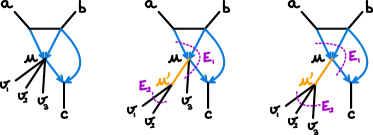
Figure 11: Left: network with a non-binary node $u$. Middle and right: refinements at $u$ for two choices of $E_{1}\mid E_{2}$. In both, $E_{1}$ contains the 3 hybrid edges incident to $u$ and $E_{2}$ contains the edges incident to $v_{1}$ and $v_{2}$. The edge incident to $v_{3}$ is either in $E_{1}$ (middle) or in $E_{2}$ (right). The canonical refinement at $u$ is the rightmost network.

Since leaves must have degree one and refinements are defined at non-binary nodes, $u$ cannot be a leaf. Also, if either $E_{1}$ or $E_{2}$ has only one edge, then $u$ or $u^{\prime}$ would become of degree 2, rendering the refinement uninteresting. It is easy to see that $N^{\prime}$ is still a valid semidirected network, since for any rooted network $N^{+}$ that induces $N$, one can keep the root and direct the new edges consistently to get a rooted network ${N^{+}}^{\prime}$ that induces $N^{\prime}$. Namely, if $u$ is a hybrid node, then $uu^{\prime}$ is directed towards $u^{\prime}$. Otherwise, we can direct $uu^{\prime}$ depending on whether the single parent of $u$ is in $E_{1}$ or in $E_{2}$. In both cases, $uu^{\prime}$ is a tree edge.

A blob-preserving refinement does not change the non-trivial blobs, but adds a new trivial blob $\{u^{\prime}\}$: suppose $B$ is a non-trivial blob in $N$, then $E_{2}\subseteq E(u)\setminus E_{B}(u)$ contains cut edges only. Therefore, the new tree edge $uu^{\prime}$ is also a cut edge. The following lemma is a result of this property.

Lemma 18.

Let $B$ be a blob in a metric semidirected network $N$ on $X$, $b$ the corresponding node in the tree of blobs $T$ of $N$, and let $u$ be a non-binary node in $B$. If $N^{\prime}$ is a refinement of $N$ at $u$, then the pairwise distance on $X$ is the same on $N^{\prime}$ and $N$. Furthermore, if $N^{\prime}$ is a blob-preserving refinement at $u$ by the edge bipartition $E_{1}\mid E_{2}$, then $\text{BT}(N^{\prime})$ is a refinement of $T$ at $b$ by $\widetilde{E_{1}}\mid\widetilde{E_{2}}$, where $\widetilde{E_{2}}=E_{2}$ (which are cut-edges and appear in $T$) and $\widetilde{E_{1}}=E(b)\setminus\widetilde{E_{2}}$.

Proof: For the first claim, it suffices to show that for any tips $x,y\in X$, there is a bijection between the sets of up-down paths $x\longleftrightarrow y$ in $N$ and in $N^{\prime}$ that preserves the lengths and hybridization parameters. Assume the refinement is by $E_{1}\mid E_{2}$. Let $p$ be an up-down path between $x$ and $y$ in $N$. Consider the following map $f$. If $p$ does not include $u$, or if $p$ includes $u$ but the two edges incident to $u$ in $p$ are both in $E_{1}$, then $p$ is also an up-down path in $N^{\prime}$, and we let $f(p)=p$. If $p$ includes $u$ and the two edges incident to $u$ in $p$ are both in $E_{2}$, then we may change $u$ to $u^{\prime}$ in $p$ to obtain up-down path $p^{\prime}$ in $N^{\prime}$ and set $f(p)=p^{\prime}$. Finally, if $p$ includes $u$ with one incident edge in $E_{1}$ and one in $E_{2}$, then we may assume, without loss of generality, that $p=x\dots aub\dots y$ with $au\in E_{1}$ and $bu\in E_{2}$. Then let $p^{\prime}=x\dots auu^{\prime}b\dots y$. Since $uu^{\prime}$ is a tree edge, $p^{\prime}$ has no v-structure and is an up-down path in $N^{\prime}$. We set $f(p)=p^{\prime}$. It is easy to see that $f$ is injective, that $\gamma(f(p))=\gamma(p)$, and $\ell(f(p))=\ell(p)$. As a result, the up-down paths in the image of $f$ have hybridization parameters that sum up to one, so $f$ is surjective as well.

For the second claim, let $u^{\prime}$ be the new node introduced in the refinement. As previously noted, $E_{2}$ contains cut edges only, so we are only deleting and adding cut edges during a blob-preserving refinement. Hence all the operations correspond to the operations on the tree of blobs $T$. Consequently we can get $\text{BT}(N^{\prime})$ from $T$ by adding a node $b^{\prime}$ corresponding to the trivial blob $B^{\prime}=\{u^{\prime}\}$ in $N^{\prime}$, cut edge $bb^{\prime}$ corresponding to $uu^{\prime}$, and replace edges $bc$ with $b^{\prime}c$ for each cut edge $uv\in E_{2}$, where $c$ corresponds to the blob containing $v$. This is the refinement of $T$ at $b$ by $\widetilde{E_{1}}\mid\widetilde{E_{2}}$.

We now introduce definitions for splits that resolve a polytomy in the tree of blobs without affecting the blob itself in the network. Later, we prove that the distance split tree resolves the tree of blobs with splits of this kind.

Definition 14 (split along a blob; sibling groups).

Let $N$ be a semidirected network on $X$, $T$ its tree of blobs, and $B$ a blob of $N$ with corresponding node $b$ in $T$. When $b$ is removed, suppose $T$ is disconnected into $k$ connected components, with taxa $Y_{1},\ldots,Y_{k}$ in each. We call $\{Y_{i}\mathchar 24635\relax\;i\leq k\}$ the partition induced by $B$. If a split $\sigma$ on $X$ has a set that is the union of two or more $Y_{i}$’s, then $\sigma$ is along the partition induced by $B$, or along $B$. Let $e_{i}$ be the cut edge in $T$ (or $N$) adjacent to $B$ whose removal disconnects $Y_{i}$ from $B$. If $e_{i}$ and $e_{j}$ share a node $u\in B$ then $Y_{i}$ and $Y_{j}$ are called sibling sets of $B$ at $u$. For a node $u\in B$, the sibling group at $u$ is the union of all sibling sets of $B$ at $u$.

The following is a restatement of Lemma 3.1.7 in charles03_phylog , using our definitions.

Lemma 19.

Let $T$ be a phylogenetic $X$-tree, and $T^{\prime}$ a refinement of $T$. Then every split $\sigma\in\Sigma(T^{\prime})\setminus\Sigma(T)$ is along some node $u$ of $T$.

Next, we characterize the set of splits $\Sigma_{D}$ that satisfy the 4-point condition on $N$.

Lemma 20.

Let $N$ be a level-$1$ network on $X$ with no degree-$2$ blobs, and with internal tree edges of positive lengths. Let $B$ be a blob of $N$ of degree $4$ or more. If $B$ is trivial, then any split along $B$ satisfies the 4-point condition. If $B$ is nontrivial, then a split along $B$ satisfies the 4-point condition if and only if it is of the form $S\mid\bar{S}$ where $S$ is a union of sibling sets of $B$. Furthermore, a split $\sigma$ along $B$ is in $\Sigma(T^{\prime})$, $T^{\prime}$ being the distance split tree, if and only if $B$ is a nontrivial blob and $\sigma$ is of the form $S\mid\bar{S}$ where $S$ is a sibling group of $B$.

Proof: If $B=\{u\}$ is trivial, then for any split $\sigma$ along $B$ we can find the corresponding refinement $N^{R}$ at $u$ with the extra edge inducing $\sigma$ in the tree of blobs. Since $N^{R}$ has the same pairwise distances, $\sigma\in\Sigma(\text{BT}(N^{R}))$ satisfies the 4-point condition by lemma 17. Furthermore, we claim that for any split $\sigma$ along $B$, there is another split $\sigma^{\prime}$ along $B$ that is incompatible with $\sigma$. This would imply that $\sigma\notin\Sigma(T^{\prime})$. To show the claim, let $\{Y_{i}\mathchar 24635\relax\;i\leq d\}$ be the partition induced by $B$, with $d=\mathrm{deg}(B)\geq 4$. Let $\sigma$ be of the form $\cup_{i\in I_{1}}Y_{i}\mid\cup_{i\in I_{2}}Y_{i}$, where $\{I_{1},I_{2}\}$ is a bipartition of $\{1,\dots,d\}$. Now we may choose $\sigma^{\prime}=\cup_{i\in I_{1}^{\prime}}Y_{i}\mid\cup_{i\in I_{2}^{\prime}}Y_{i}$ where $\{I_{1}^{\prime},I_{2}^{\prime}\}$ is a bipartition of $\{1,\dots,d\}$ incompatible with $\{I_{1},I_{2}\}$: such that $I_{i}\cap I^{\prime}_{j}$ are all non-empty. Then $\sigma^{\prime}$ is along $B$ and incompatible with $\sigma$.

If $B$ is nontrivial, first consider $\sigma=S\mid\bar{S}$ where $S$ is a union of sibling sets of $B$, that is, $S$ contains the leaves corresponding to a set $E$ of cut edges adjacent to some node $u\in B$. Then, in the blob-preserving refinement of $N^{R}$ at $u$ by $E(u)\setminus E\mid E$, the extra cut edge induces $\sigma$. Hence $\sigma\in\Sigma(N^{R})$ satisfies the 4-point condition. Conversely, consider a non-trivial split $\sigma=A\mid\bar{A}$ where both $A$ and $\bar{A}$ intersect at least two of the sibling groups of $B$. Let $Y_{1},\ldots,Y_{d}$ be the sibling groups such that $Y_{1}$ is the sibling group at $B$’s hybrid node. Since $d=\mathrm{deg}(B)\geq 4$, it is easy to see that we can find distinct $\{i_{1},\ldots,i_{4}\}$, $x_{1},x_{2}\in A$ and $x_{3},x_{4}\in\bar{A}$ such that $1\in\{i_{1},\ldots,i_{4}\}$, and $x_{j}\in Y_{i_{j}}$. Then the subnetwork $\tilde{N}=N_{\{x_{1}x_{2}x_{3}x_{4}\}}$ is equivalent to the leftmost network in Figure 8 with positive branch lengths for both tree edges in the cycle. By Example 3, the 4-point condition is not met for $x_{1}x_{2}\mid x_{3}x_{4}$, which finishes the proof of the claim.

Finally, consider a split $\sigma=S\mid\bar{S}$ along $B$ that satisfies the 4-point condition, but where $S$ is a proper subset of the sibling group at some node $u\in B$. Then $u$ must be adjacent to $k\geq 3$ cut edges, and $S$ must be the union of $l$ sibling sets at $u$, with $2\leq l<k$. Then similarly to the case when $B$ is trivial, we can find a nonempty union of sibling sets $S^{\prime}$, such that $\sigma^{\prime}=S^{\prime}\mid\bar{S}^{\prime}$ is incompatible with $\sigma$. Since $\sigma^{\prime}$ satisfies the 4-point condition, $\sigma\notin\Sigma(T^{\prime})$.

Proof: [Proof of Theorem 10] Note that the procedure described to obtain $N^{R}$ is a series of canonical refinements. So by Lemma 18, $N^{R}$ is a valid semidirected network with average distances identical to those in $N$.

Let $T=\text{BT}(N)$ and $T^{\prime}$ the distance split tree of $N$. By Lemma 19, any split $\sigma\in\Sigma(T^{\prime})\setminus\Sigma(T)$ is along some blob $B$ of $N$. By Lemma 20, there is no such extra split $\sigma$ when $B$ is trivial. If $B$ is nontrivial, the extra splits must be of the form $S\mid\bar{S}$ where $S$ is a sibling group at some node $u$. Such a split corresponds to the split introduced in the canonical refinement at $u$.

Finally, since $N^{R}$ can be obtained from a series of canonical refinements, by Lemma 18, the tree of blobs of $N^{R}$ can also be obtained from the series of corresponding refinements, which introduces exactly all the extra splits described above. As a result, $\text{BT}(N^{R})=T^{\prime}$.

5 Identifying sunlets

A $k$-sunlet is a semidirected network with a single $k$-cycle and reticulation, and for each node on the cycle, one or more pendant edge(s) (adjacent to a leaf). The sunlet is binary if $k$ equals the number of leaves, $n$. This section considers the problem of identifying the branch lengths and hybridization parameters in a sunlet from the average distances between the $n$ tips. We assume that we know the network is a $k$-sunlet, but $k$ is unknown and the ordering of the tips around the cycle is unknown. In other words, we consider the problem of identifying the exact network topology given that it is a sunlet.

A circular ordering of the leaves $X=\{x_{1},\ldots,x_{k}\}$ is, informally, the order of the leaves when placed around an undirected cycle. Formally, it is the class of an ordering $(x_{i_{1}},\ldots,x_{i_{k}})$ up to the equivalence relations $(u_{1},\ldots,u_{k})\sim(u_{k},\ldots,u_{1})$ and $(u_{1},u_{2},\ldots,u_{k})\sim(u_{2},\ldots,u_{k},u_{1})$.

5.1 4-sunlets

First we consider the problem of identifying the lengths and hybridization parameter in a binary $4$-sunlet, assuming the labelled semidirected topology is known (Fig. 12 left). Specifically, we assume that we know $h$ is of hybrid origin, $a$ and $b$ are its half-sisters and $g$ is opposite of the hybrid node.

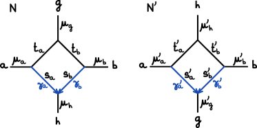
Figure 12: $4$-sunlets with the same undirected topology. Left: $h$ is of hybrid origin. Right: $g$ is of hybrid origin. By Theorem 22, parameters can be chosen such that both networks have the same average distances between leaves.

In this case, we have $6$ average distances, but $9$ parameters. Zipping up the $4$-sunlet removes $2$ degrees of freedom, but one free parameter still remains. Specifically, we have

$$\begin{split}d_{ga}&=(\mu_{a}+t_{a})+\mu_{g}\\ d_{gb}&=(\mu_{b}+t_{b})+\mu_{g}\\ d_{ab}&=(\mu_{a}+t_{a})+(\mu_{b}+t_{b})\\ d_{ah}&=(\mu_{h}+s_{a}\gamma_{a}+s_{b}\gamma_{b})+\gamma_{b}(t_{a}+t_{b})+\mu_{a}\\ d_{bh}&=(\mu_{h}+s_{a}\gamma_{a}+s_{b}\gamma_{b})+\gamma_{a}(t_{a}+t_{b})+\mu_{b}\\ d_{gh}&=(\mu_{h}+s_{a}\gamma_{a}+s_{b}\gamma_{b})+\gamma_{a}t_{a}+\gamma_{b}t_{b}+\mu_{g}\end{split}$$ (5)

Theorem 21.

Let $d$ be a metric on four tips $\{a,b,g,h\}$. The $4$-sunlet $N$ with circular ordering $(a,g,b,h)$ and in which $h$ is of hybrid origin (left of Fig. 12) has average distances $d$ for some set of parameters such that $t_{a}>0$ and $t_{b}>0$ if and only if

$$d_{gh}+d_{ab}>\max\{d_{ah}+d_{bg},d_{bh}+d_{ag}\}$$ (6)

and

$$\frac{d_{gh}+d_{ab}-d_{ah}-d_{bg}}{d_{ab}+d_{ag}-d_{bg}}+\frac{d_{gh}+d_{ab}-d_{bh}-d_{ag}}{d_{ab}+d_{bg}-d_{ag}}\leq 1.$$ (7)

In this case, we can identify $\mu_{g}$ and the following composite parameters:

$$\begin{split}\mu_{g}&=\frac{1}{2}(d_{ag}+d_{bg}-d_{ab})\\ \mu_{a}+t_{a}&=\frac{1}{2}(d_{ab}+d_{ag}-d_{bg})\\ \mu_{b}+t_{b}&=\frac{1}{2}(d_{ab}+d_{bg}-d_{ag})\\ l_{h}:=\mu_{h}+s_{a}\gamma_{a}+s_{b}\gamma_{b}&=\frac{1}{2}(d_{ah}+d_{bh}-d_{ab})\\ \gamma_{a}t_{a}&=\frac{1}{2}(d_{gh}+d_{ab}-d_{ah}-d_{bg})\\ \gamma_{b}t_{b}&=\frac{1}{2}(d_{gh}+d_{ab}-d_{bh}-d_{ag})\;.\end{split}$$ (8)

However, $\gamma$, $t_{a}$, $t_{b}$, $\mu_{a}$, $\mu_{b}$ are not identifiable. In particular, $\gamma_{a}$ can take any value in the following interval:

$$\left[\frac{d_{gh}+d_{ab}-d_{ah}-d_{bg}}{d_{ab}+d_{ag}-d_{bg}}\;,\;1-\frac{d_{gh}+d_{ab}-d_{bh}-d_{ag}}{d_{ab}+d_{bg}-d_{ag}}\right]\,.$$

Furthermore, (6) is an equality if and only if one of the tree edges in the cycle has zero length: $t_{a}=0$ or $t_{b}=0$.

The proof below uses basic algebra. Condition (7) ensures that (8) can be solved to give non-negative $\mu_{a}$ and $\mu_{b}$, and (6) ensures that $\gamma_{a}t_{a}>0$ and $\gamma_{b}t_{b}>0$. If (6) is an equality, then the 4-point condition is satisfied and $d$ is a tree metric. $\gamma_{a}=0$ or $1$ lead to a tree metric, but hybrid edges are required to have $\gamma>0$ by definition. Setting $t_{a}$ or $t_{b}$ to $0$ also leads to a tree metric. Contracting the corresponding edge creates an unidentifiable degree-3 blob.

Proof: [Proof of Theorem 21] It is easy to check with basic algebra that (8) is equivalent to (5). Therefore, we simply need to show that additionally imposing (6) and (7) is equivalent to requiring edge lengths be non-negative, $t_{a},t_{b}>0$ and hybridization parameters be in $(0,1)$. Suppose that $d$ comes from the $4$-sunlet $N$. Condition (6) is equivalent to $d_{gh}+d_{ab}-d_{ah}-d_{bg}=2\gamma_{a}t_{a}\geq 0$ and $d_{gh}+d_{ab}-d_{bh}-d_{ag}=2\gamma_{b}t_{b}\geq 0$. For condition (7), we have

$$\frac{d_{gh}+d_{ab}-d_{ah}-d_{bg}}{d_{ab}+d_{ag}-d_{bg}}+\frac{d_{gh}+d_{ab}-d_{bh}-d_{ag}}{d_{ab}+d_{bg}-d_{ag}}=\frac{\gamma_{a}t_{a}}{\mu_{a}+t_{a}}+\frac{\gamma_{b}t_{b}}{\mu_{b}+t_{b}}\leq 1.$$

Conversely, suppose that a metric $d$ on $\{a,g,b,h\}$ satisfies (6) and (7). Then there exists $\tilde{\gamma}$ such that

$$0<\frac{d_{gh}+d_{ab}-d_{ah}-d_{bg}}{d_{ab}+d_{ag}-d_{bg}}\leq\tilde{\gamma}\leq 1-\frac{d_{gh}+d_{ab}-d_{bh}-d_{ag}}{d_{ab}+d_{bg}-d_{ag}}<1\,.$$

Then we can set $\gamma_{a}=1-\gamma_{b}=\tilde{\gamma}$ in (8) to solve for $t_{a}$ first, getting $t_{a}>0$ from (6). Then solving for $\mu_{a}$, we get

$$\mu_{a}=\frac{1}{2}\left((d_{ab}+d_{ag}-d_{bg})-(d_{gh}+d_{ab}-d_{ah}-d_{bg})/\tilde{\gamma}\right)\geq 0$$

because of our condition on $\tilde{\gamma}$. Similarly, solving for $t_{b}$ and $\mu_{b}$ gives $t_{b}>0$ and $\mu_{b}\geq 0$.

When the sunlet topology is unknown, we need to identify the circular ordering of the tips around the cycle, and which of $a,b,g$ or $h$ is of hybrid origin. Suppose the tips are labelled by $x,y,z,w$, then by Theorem 21, the opposing pairs $\{x,y\}$ and $\{z,w\}$ correspond to the largest sum among $d_{xy}+d_{zw}$, $d_{xz}+d_{yw}$ and $d_{xw}+d_{yz}$.

Identifying the opposing pairs $\{a,b\}$ and $\{g,h\}$ is enough to identify the undirected graph of the $4$-sunlet. However, identifying which tip is of hybrid origin is impossible, as we show below.

Theorem 22.

Let $N$ be the $4$-sunlet with circular ordering $(a,g,b,h)$ in which $h$ is of hybrid origin (Fig. 12, left). Let $N^{\prime}$ be the $4$-sunlet with the same circular ordering, but in which $g$ is of hybrid origin (Fig. 12, right). For any parameters $(\ell,\gamma)$ on $N$, there exist parameters $(\ell^{\prime},\gamma^{\prime})$ on $N^{\prime}$ such that $N$ and $N^{\prime}$ have the same average distances.

Proof: We apply Theorem 21 to $N^{\prime}$ and the distance $d$ obtained from $N$. We need to check that (6) and (7) are met. Condition (6) is met because it is symmetric in $g$ and $h$. Condition (7) is not symmetric however. To fit $d$ on $N^{\prime}$, (7) can be written as (after permuting $g$ and $h$):

$$\frac{d_{gh}+d_{ab}-d_{ag}-d_{bh}}{d_{ab}+d_{ah}-d_{bh}}+\frac{d_{gh}+d_{ab}-d_{bg}-d_{ah}}{d_{ab}+d_{bh}-d_{ah}}\leq 1\,.$$

Applying (8) to $N$ from which $d$ is obtained, we can rewrite the left-hand side as:

$$\frac{\gamma_{b}t_{b}}{(\mu_{a}+t_{a})-\gamma_{a}t_{a}+\gamma_{b}t_{b}}+\frac{\gamma_{a}t_{a}}{(\mu_{b}+t_{b})-\gamma_{b}t_{b}+\gamma_{a}t_{a}}=\\ \frac{\gamma_{b}t_{b}}{\mu_{a}+\gamma_{b}(t_{a}+t_{b})}+\frac{\gamma_{a}t_{a}}{\mu_{b}+\gamma_{a}(t_{a}+t_{b})}\leq\frac{\gamma_{b}t_{b}}{\gamma_{b}(t_{a}+t_{b})}+\frac{\gamma_{a}t_{a}}{\gamma_{a}(t_{a}+t_{b})}=1\,.$$

Hence (7) is met on $N^{\prime}$, and parameters can be set to match the average distances from $N$.

Depending on the parameters in the $4$-sunlet, it may be possible to switch $g$ with $a$ and $h$ with $b$ as well, if condition (7) holds for the network in which $a$ (or $b$) is of hybrid origin. Namely, this is possible if $\mu_{h}$ and $\mu_{g}$ are large enough to satisfy

$$\frac{\gamma_{a}t_{a}}{\mu_{g}+\gamma_{a}t_{a}}+\frac{\gamma_{b}t_{b}}{\mu_{h}+s_{a}\gamma_{a}+s_{b}\gamma_{b}+\gamma_{b}t_{b}}\leq 1.$$

Usually we do not have external information about which tip is of hybrid origin, and even if we do, by Theorem 21 we can only identify $\mu_{g}$, the length of the branch “across” from the hybrid node. It is therefore not possible to identify the individual edge lengths. More generally, we can combine the swap lemma and Theorem 21 to prove that almost any hybrid-closed subgraph with 4 boundary nodes can be swapped with a 4-cycle without affecting distances.

Proposition 23 (swap a subgraph with a 4-sunlet).

In a network $N$, let $A$ be a hybrid-closed connected subgraph with 4 boundary nodes such that $\gamma_{A}\equiv 1$ and each node $u\in\partial A$ has degree 1 in $A$. Let $t(u)$ denote the length of the edge incident to $u$ in $A$. Then there exists $\eta\geq 0$ (which depends on $A\setminus\partial A$) such that the following holds: If $t(u)\geq\eta$ for each $u\in\partial A$, then we can swap $A$ with a tree or with a 4-sunlet $A^{\prime}$ on leaf set $\partial A$ to obtain a valid semidirected network $N^{\prime}$ with $d_{N^{\prime}}=d_{N}$.

Proof: To simplify notations, let $d$ denote $d(.,.\mid A)$. If $d$ satisfies the 4-point condition, then there is a unique 4-taxon tree $A^{\prime}$ on $\partial A$ such that $d_{A^{\prime}}=d$ on $\partial A$ (and $\gamma_{A^{\prime}}\equiv 1$). Swapping $A$ with $A^{\prime}$ leads to a valid semidirected network topology $N^{\prime}$ because any valid root position in $N$ remains valid in $N^{\prime}$. $N^{\prime}$ remains acyclic because $\gamma_{A}\equiv 1$ and $A$ is hybrid-closed: when edges are directed away from the root, $A$ must have exactly one “entry” boundary node, whose incident edge in $A$ is outgoing. Therefore, an undirected path between two nodes in $\partial A$ made of edges not in $A$ must have a v-structure, and then $N^{\prime}$ cannot contain directed cycles. Finally, we can apply Lemma 15 to prove the claim with $\eta=0$.

If $d$ does not satisfy the 4-point condition, then $A$ must contain at least one hybrid edge. We may label the nodes in $\partial A$ as $\{h,a,g,b\}$ such that (6) holds for $d$ and $h$ is below some hybrid edge in $A$. Let $A^{\prime}$ be a 4-sunlet on leaf set $\partial A$ with $h$ below the hybrid node and circular ordering $(h,a,g,b)$. Swapping $A$ with $A^{\prime}$ leads to a valid semidirected network topology $N^{\prime}$ because any valid root position in $N$ is not below $h$, and is again valid in $N^{\prime}$. We also have $\gamma_{A^{\prime}}=\gamma_{A}\equiv 1$. We now want to assign edge parameters in $A^{\prime}$ such that $d_{A^{\prime}}=d$ on $\partial A$. By Theorem 21, this is possible provided that (7) holds for $d$. Modifying $t(u)$ for $u\in\partial A$ does not modify the numerator of either term in (7). Let $aa_{0}$ and $b_{0}b$ be the edges in $A$ incident to $a$ and $b$ respectively. Then the denominators in (7) can be expressed as $2t(a)+d_{a_{0}b_{0}}+d_{a_{0}g}-d_{b_{0}g}$ and $2t(b)+d_{a_{0}b_{0}}+d_{b_{0}g}-d_{a_{0}g}$. Therefore (7) holds if $t(a)>\eta$ and $t(b)>\eta$ where $\eta$ is the maximum of $d_{gh}+d_{a_{0}b_{0}}-d_{a_{0}h}-d_{b_{0}g}-(d_{a_{0}b_{0}}+d_{a_{0}g}-d_{b_{0}g})/2$ and $d_{gh}+d_{a_{0}b_{0}}-d_{b_{0}h}-d_{a_{0}g}-(d_{a_{0}b_{0}}+d_{b_{0}g}-d_{a_{0}g})/2$. This concludes the proof by Lemma 15.

We can now prove Theorem 7 on networks of level up to $k$, $k\geq 2$.

Proof: [Proof of Theorem 7] It suffices to consider $k=2$. Consider the networks in Fig. 8, say $A_{1}$ on the left and $A_{2}$ on the right. Let $n\geq 4$. If $n=4$, set $N_{1}=A_{1}$ and $N_{2}=A_{2}$. If $n\geq 5$, we can form networks $N_{i}$ ($i=1,2$) with $n$ taxa by replacing the leaves $a$, $b$, $c$ and/or $d$ in $A_{i}$ by subtrees with enough taxa. Given any values for the parameters labelled in Fig. 8 for $A_{2}$ such that $u_{4}>0$, $d_{A_{2}}$ satisfies (6) with the same ordering as $d_{A_{1}}$. By Proposition 23 and its proof, we can swap $A_{2}$ with $A_{1}$ provided that the edges incident to $b$ and $c$ are long enough in $A_{2}$. It follows that $d_{N_{1}}=d_{N_{2}}$ for parameters in subsets of positive Lebesgue measure.

Definition 15 (canonical 4-sunlet split network).

Consider a 4-sunlet whose undirected topology has circular ordering $(a,g,b,h)$ (e.g. Fig. 13 right) and with cycle tree edges of positive lengths. The underlying undirected graph (e.g. Fig. 13 left) can be considered as a split network, in which each pair of parallel edges identifies a single split and a single split weight (edge length), with canonical edge lengths defined as follows.

$$\hat{\mu}_{g} =\frac{1}{2}(d_{ga}+d_{gb}-d_{ab}) \hat{\mu}_{a} =\frac{1}{2}(d_{ag}+d_{ah}-d_{gh})$$

$$\hat{\mu}_{h} =\frac{1}{2}(d_{ha}+d_{hb}-d_{ab}) \hat{\mu}_{b} =\frac{1}{2}(d_{bg}+d_{bh}-d_{gh})$$ (9)

$$\hat{t}_{hb\mid ga} =\frac{1}{2}(d_{gh}+d_{ab}-d_{ga}-d_{hb}) \hat{t}_{ha\mid gb} =\frac{1}{2}(d_{gh}+d_{ba}-d_{gb}-d_{ha})\,.$$

Distances on this canonical split network, calculated between any two tips as the length of the shortest path between them huson_rupp_scornavacca_2010 , are identical to the average distances on the original semi-directed 4-sunlet.

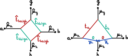
Figure 13: Left: split network, with canonical edge lengths from Definition 15. A pair of parallel edges represent the same split and thus share the same length ($\hat{t}_{hb\mid ga}$ or $\hat{t}_{ha\mid gb}$ here). The distance between two nodes is defined as the length of the shortest path between them. Right: example zipped-up $4$-sunlet represented by the split network on the left, in which $h$ is of hybrid origin. Distances (using up-down paths) are identical to distances on the split network and satisfy (5.1).

This split network provides a unique representation of what can be identified from pairwise distances: undirected topology and identifiable composite parameters. Ideally, we would have liked a semi-directed representation, but since the location of the hybrid node is not identifiable, this was not an option.

Theorem 24 (identifiability of $4$-sunlet split network).

Let $N$ and $N_{0}$ be binary $4$-sunlets with identical leaf set and internal tree edges of positive lengths. If $N$ and $N_{0}$ have identical average distances, then the canonical $4$-sunlet split networks of $N$ and $N_{0}$ are identical.

Proof: The positivity of cycle tree edge lengths ensures that

$$d_{ab}+d_{gh}>\max\{d_{ag}+d_{bh},d_{ah}+d_{bg}\}$$

is satisfied strictly, so $N$ and $N_{0}$ must have the same circular ordering. Finally, the definition of canonical edge lengths from average distances in (15) is symmetric with respect to the hybrid node: canonical lengths depend on the circular ordering only. There is a tight correspondence between edge lengths in the semi-directed network and edge lengths in the split network, provided that the placement of the hybrid node is known. For example, if $h$ is of hybrid origin and if the network is zipped up as in Fig. 13 (right), then by Theorem 21 we have that:

$$\hat{\mu}_{g} =\mu_{g}, \hat{\mu}_{a} =\mu_{a}+\gamma_{b}t_{a}, \hat{t}_{ha\mid gb} =\gamma_{a}t_{a},$$

$$\hat{\mu}_{h} =\mu_{h}, \hat{\mu}_{b} =\mu_{b}+\gamma_{a}t_{b}, \hat{t}_{hb\mid ga} =\gamma_{b}t_{b}.$$ (10)

By (5.1) we have that $\hat{\mu}_{s}\geq\mu_{s}$ for each cut edge. In fact, $\hat{\mu}_{s}=\mu_{s}$ is a correct length estimate for the zipped-up child edge of the hybrid node and for the cut edge opposite to the hybrid node. For the other cut edges, $\hat{\mu}_{s}$ is an overestimate of $\mu_{s}$. For example, for the network in Fig. 13 (right) where $h$ is the hybrid node, then $\hat{\mu}_{a}=\mu_{a}+\gamma_{b}t_{a}\geq\mu_{a}$. We do not know which cut edge length is correctly represented, however. Similarly, $\hat{t}_{hb\mid ga}$ and $\hat{t}_{ha\mid gb}$ are underestimates of the length of tree edges in the cycle, although we do not know which edges in the cycle are tree or hybrid edges.

If a 4-sunlet has a polytomy, its canonical split network can be defined (and Theorem 24 can be applied) after resolving the polytomy with an extra edge of length 0. As Fig. 14 shows, networks with polytomies adjacent to a 4-cycle may have the same average distances as networks without polytomies.

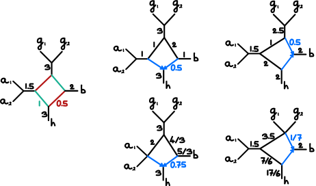
Figure 14: Canonical split network representation (left) of 4 zipped-up semidirected networks with identical average distances, in which $h$ (middle) or $b$ (right) is of hybrid origin. Two networks (bottom) have a polytomy adjacent to the 4-cycle. In the split network, pairs of parallel edges of identical color represent a single split and share the same length (split weight). Hybrid edges (arrows) have length $0$ and inheritance $\gamma$ shown in blue for one of them. Numbers in black indicate edge lengths. The split network shows the 6 composite parameters identifiable from distances, pertaining to the 4-cycle. Zipped-up semidirected networks have 7 associated parameters.

5.2 $k$-sunlet for $k\geq 5$

With $5$ or more nodes in the cycle, we can identify the topology, branch lengths, and hybridization parameters of the zipped-up version of the sunlet.

Theorem 25 ($k$-sunlet identifiability, $k\geq 5$).

Let $N$ and $N_{0}$ be semidirected networks with identical leaf set $\{u_{0},\ldots,u_{n-1}\}$ and internal tree edges having positive lengths, such that $N$ is a $k$-sunlet and $N_{0}$ is a $k_{0}$-sunlet with $k_{0}\geq 5$. If $N$ and $N_{0}$ have identical average distances, then the zipped-up versions of $N$ and $N_{0}$ are identical.

Proof: We first we show that $N$ and $N_{0}$ must have the same topology, and then the same branch lengths and hybridization parameter. In $N_{0}$, let the hybrid node be $v_{0}$, and let the other internal nodes be $v_{1},\ldots,v_{k-1}$ such that $v_{i-1}$ and $v_{i}$ are neighbors (as in Fig. 15). Let $C_{i}$ be the set of leaves adjacent to $v_{i}$ in $N_{0}$. If there are no polytomies, then each $C_{i}$ is reduced to a single leaf $u_{i}$.

Figure 15: Left: $5$-sunlet $N$ on $8$ taxa. Its tree of blobs is a star. $C_{i}$ is the sibling group at $v_{i}$ ($i=0,\dots,4$). Right: distance split tree constructed from $d_{N}$. It is a refinement of the tree of blobs, but identifies the polytomies in the sunlet.

By Lemma 20, each non-trivial split in the distance split tree of $N$ is of the form $C\mid\bar{C}$, where $C$ is a set of all the sister leaves that are adjacent to the same cycle node in $N$, and $\bar{C}=X\setminus C$. The same holds for $N_{0}$.

Since $N$ and $N_{0}$ have identical pairwise distances, they have the same distance split tree, and consequently identical sets of sister leaves (polytomies). In particular, we must have that $k=k_{0}$. So without loss of generality, we choose a single representative leaf from each $C_{i}$ for the remainder of the proof. In other words, we may assume that both $N$ and $N_{0}$ have no polytomies and $k=n$ (as in Fig. 16).

Identifying the circular ordering of leaves.

First, we claim that the leaf of hybrid origin $u_{0}$ is the only leaf $u$ such that:

$$\forall x,y,z,\{u,x,y,z\}\mbox{ does \emph{not} satisfy the 4-point condition.}$$ (11)

Indeed, if $u=u_{0}$, then $\{u,x,y,z\}$ induces in $N_{0}$ a 4-sunlet in which both tree edges in the cycle have positive length, so $\{u,x,y,z\}$ does not satisfy the 4-point condition by Theorem 21. If $u=u_{i}$ for $i>0$, then we can choose $3$ other leaves $u_{j}$, $u_{k}$, $u_{l}$ different from $u_{0}$, because $k_{0}\geq 5$. The induced subnetwork is then a tree, so the 4-point condition holds, such that $u_{i}$ does not satisfy (11) for $i\geq 0$. Therefore, the leaf of hybrid origin must be the same in $N$ as in $N_{0}$: $u_{0}$.

Next, we consider the subnetwork of $N_{0}$ induced by the leaves other than $u_{0}$. (For sake of brevity, in what follows in this subsection, all the subnetworks have degree-$2$ nodes suppressed.) This subnetwork has no reticulation, it is binary and its internal branch lengths are positive, so it is equal to its tree of blobs and its distance split tree. Therefore, the subnetwork of $N$ induced by the leaves other than $u_{0}$ has the same tree topology. This tree must be a caterpillar (Fig. 16, middle) with two cherries: $\{u_{1},u_{2}\}$ and $\{u_{k-2},u_{k-1}\}$ and internal nodes that correspond to $v_{2},\ldots,v_{k-2}$. Its topology determines the ordering of the other leaves. In other words, the ordering of $u_{3},\ldots,u_{k-3}$ must be identical in $N$ and in $N_{0}$. We can also match the internal nodes $v_{3},\ldots,v_{k-3}$ in $N_{0}$ to internal nodes in $N$. What remains to be identified is which of $\{u_{1},u_{2}\}$ and which of $\{u_{k-2},u_{k-1}\}$ is adjacent to either parent of the hybrid node in $N$. For this, consider the subnetworks from $N$ and $N_{0}$ induced by $\{u_{2},u_{1},u_{0},u_{k-1}\}$. By (6) in Theorem 21, the average distances on $\{u_{0},u_{1},u_{2},u_{k-1}\}$ determine the circular ordering of these 4 taxa, such that $u_{1}$ must be adjacent to a hybrid parent in $N$, as it is in $N_{0}$. Similarly, the average distances on $\{u_{0},u_{1},u_{k-2},u_{k-1}\}$ determine the circular ordering of these 4 taxa such that $u_{k-1}$ must be adjacent to a hybrid parent in $N$, like in $N_{0}$. This finishes the proof that the circular ordering of leaves is identical in $N$ and in $N_{0}$.

Figure 16: Left: binary $k$-sunlet. Middle: after excluding $u_{0}$, the subnetwork is a tree. Right: subnetwork on $\{u_{0},u_{1},u_{2},u_{k-2},u_{k-1}\}$, a sunlet with $k=5$.

Identifying branch lengths and hybridization parameters.

By considering distances between $u_{1},\ldots,u_{k-1}$, we can determine the lengths of all the edges of the caterpillar tree $N_{\{u_{1}\ldots,u_{k-1}\}}$ (Fig. 16, middle). In particular, we get that the following edges have the same length in $N$ as in $N_{0}$: $v_{i}v_{i+1}$ for $2\leq i\leq k-3$ and $v_{i}u_{i}$ for $2\leq i\leq k-2$. The parameters that remain to be identified are in the subnetwork induced by $\{u_{0},u_{1},u_{2},u_{k-2},u_{k-1}\}$. Therefore, we may assume that $k=5$, as we do below (Fig. 16, right).

For brevity in this paragraph, for an edge $uv$ we also write its length as $uv$. From the tree induced by $\{u_{1},\ldots,u_{4}\}$, we have the lengths $u_{2}v_{2}$, $u_{3}v_{3}$, $v_{2}v_{3}$, $v_{3}v_{4}+u_{4}v_{4}$, and $u_{1}v_{1}+v_{1}v_{2}$. From the subnetwork induced by $\{u_{0},u_{1},u_{2},u_{4}\}$, by Theorem 21 we can identify $l_{h}=\gamma_{1}\cdot v_{1}v_{0}+\gamma_{4}\cdot v_{4}v_{0}+u_{0}v_{0}$, which is the length of $v_{0}u_{0}$ after unzipping. We can also identify $\gamma_{1}\cdot v_{2}v_{1}$ and $\gamma_{4}(v_{2}v_{3}+v_{3}v_{4})$. From the subnetwork on $\{u_{0},u_{1},u_{3},u_{4}\}$, we also get $\gamma_{1}(v_{1}v_{2}+v_{2}v_{3})$. Hence we can identify $\gamma_{1}$ as $\big{(}\gamma_{1}(v_{1}v_{2}+v_{2}v_{3})-\gamma_{1}\cdot v_{1}v_{2}\big{)}/v_{2}v_{3}$ from pairwise distances. All other parameters in the unzipped version of $N$ are also identifiable, using: $v_{1}v_{2}=\gamma_{1}\cdot v_{1}v_{2}/\gamma_{1}$, $\gamma_{4}=1-\gamma_{1}$, $v_{3}v_{4}=\big{(}\gamma_{4}(v_{2}v_{3}+v_{3}v_{4})\big{)}/\gamma_{4}-v_{2}v_{3}$, and as a result $u_{1}v_{1}$ and $u_{4}v_{4}$.

6 Identifying level-1 networks

While a degree-3 blob is not detectable, a $4$-cycle in a level-$1$ network corresponds to a polytomy in the tree of blobs. Its hybrid node and its zipped-up version is unidentifiable, but the canonical split network of a 4-sunlet is identifiable, by Theorem 24. To prove Theorem 12, we first define mixed networks formally.

6.1 Mixed network representation

In the mixed representation of a semi-directed level-1 network, the cycles of size $5$ or greater are unchanged. The $4$-cycles, which are only partially identifiable, are replaced by split networks, extending the split network representation of $4$-sunlets from section 5.1 with canonical edge lengths given by (15).

Definition 16 (mixed network).

A mixed network is a semidirected graph where undirected edges are partitioned into two sets: tree edges $E_{T}$ and split edges $E_{S}$; and where $E_{S}$ is itself partitioned into a set of classes. When the graph is embedded in a Euclidean space, split edges within the same class are represented as parallel segments. A metric $(\ell,\gamma)$ on a mixed network $M$ is such that $\ell:E\to\mathbb{R}_{\geq 0}$ assigns the same length to all edges in the same class of split edges; and $\gamma:E\to[0,1]$ assigns $\gamma(e)=1$ if $e$ is undirected and $\gamma(e)\in(0,1)$ if $e$ is directed.

Definition 17 (mixed network representation of a level-1 network).

Let $N$ be a level-$1$ semidirected network with no $2$- or $3$-cycles. The mixed network representation $N^{*}$ of $N$ is the mixed network obtained as follows:

1. In each $4$-cycle, the subgraph on the left of Fig. 17 is excised and replaced with that on the right.

2. Suppress any degree-$2$ node.

In $N^{*}$, $4$-cycles consist of split edges and are called split blobs.

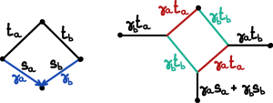
Figure 17: Mixed network: representation of a $4$-cycle in a semidirected network $N$ (left) to form a split blob (right). Edges in the cycle are converted to undirected split edges with $\gamma=1$, categorized in two classes depicted by colors. Adjacent tree edges are added. If $N$ is zipped up, then $s_{a}=s_{b}=0$ and the lower tree edge (adjacent to the hybrid node in $N$) is not needed.

In a mixed network $M$, a mixed up-down path between two nodes $a,b$ is a path $p=u_{0}u_{1}\dots u_{n}$ between $u_{0}=a$ and $u_{n}=b$ in $U(M)$ such that:

1. $p$ has no v-structure, that is, no segment $u_{i-1}u_{i}u_{i+1}$ such that $(u_{i-1}u_{i})$ and $(u_{i+1}u_{i})$ are directed edges in $M$;

2. if a segment $u_{i}\dots u_{j}$ consists solely of split edges, then the segment is a shortest path between $u_{i}$ and $u_{j}$ in $U(M)$.

Given a metric $(\ell,\gamma)$ on $M$, the length of $p$ is $\ell(p)=\sum_{e\in p}\ell(e)$, and the probability of $p$ is $\gamma(p)=\prod_{e\in p}\gamma(e)$. A split segment is a path that consists solely of split edges. Two split segments $S_{1},S_{2}$ are equivalent if they have the same endpoints and $\ell(S_{1})=\ell(S_{2})$. Note that a split segment $S$ must have $\gamma(S)=1$. Two mixed up-down paths $p$ and $q$ are equivalent if one can obtain $q$ from $p$ by replacing some split segments of $p$ by equivalent split segments.

Definition 18 (average distance in a mixed network).

The average distance between two nodes $u,v$ in a mixed network $M$ is the weighted average length of mixed up-down paths, up to equivalence, between $u$ and $v$:

$$d_{M}(u,v)=\sum_{p\in P_{uv}}\gamma(p)\ell(p)$$

where $P_{uv}$ is a set of mixed up-down paths between $u$ and $v$, containing exactly one representative from each equivalence class. This distance is well-defined because equivalent paths have the same lengths and probabilities.

Importantly, average distances are preserved by the mixed representation of a level-1 network:

Theorem 26.

Let $N$ be a level-$1$ semidirected network on taxon set $X$, and $N^{*}$ the mixed network representation of $N$. Then for any $x,y\in X$,

$$d_{N}(x,y)=d_{N^{*}}(x,y).$$

The proof, in appendix A.4, first shows that average distances in mixed networks can be interpreted as the expected shortest path length over “displayed split networks”.

6.2 Identifying the mixed representation of level-1 networks

We now have the tools to prove Theorem 12.

Proof: [Proof of Theorem 12] For $i=1,2$, let $N_{i}$ be a zipped-up level-1 semidirected network on $X$ with internal tree edges of positive lengths, and $N_{i}^{R}$ the refinement described in Theorem 10. Also let $N_{i}^{R*}$ be the mixed representation of $N_{i}^{R}$, and $N_{i}^{*}$ the mixed representation of $N_{i}$. Assume that $d_{N_{1}}=d_{N_{2}}=d$. By Theorem 10, $N_{1}^{R}$ and $N_{2}^{R}$ have the same tree of blobs $T$, so their blobs and cut edges are in bijection.

Let $b$ be a node of degree $k\geq 4$ in $T$, and $\{e_{1},\ldots,e_{k}\}$ be the cut edges incident to $b$ in $T$. Let $B_{i}$ be the corresponding cycle in $N_{i}^{R}$ ($i=1,2$), of length $k\geq 4$. Removing $e_{j}$ disconnects $T$ into two components. We select a leaf $x_{j}$ from the component that does not contain $b$ and use distances on $\{x_{1},\ldots,x_{k}\}$. If $k\geq 5$, $B_{1}$ and $B_{2}$ have the same topology and edge parameters by Theorem 25. If $k=4$, the split cycle representing $B_{1}$ (in $N_{1}^{R*}$) and $B_{2}$ (in $N_{2}^{R*}$) have the same topology and canonical length of split edges, by Theorem 24. So $N_{1}^{R*}$ and $N_{2}^{R*}$ have the same topology (referred below as $N^{R*}$) and same parameters for edges within a blob.

Next, we need to prove that cut edges have the same length in $N_{1}^{R*}$ and $N_{2}^{R*}$. These edges are also cut edges in $N_{i}^{R}$ ($i=1,2$) and $T$. Let $e=uv$ be a cut edge and $B(u),B(v)$ the blobs that $u$ and $v$ belong to. We can select leaves as follows. If $B(u)=\{u\}$ (resp. $B(v)=\{v\}$) is an internal tree node that is not in any cycle, let $e_{1}$ and $e_{2}$ (resp. $e_{3}$ and $e_{4}$) be the two cut edges incident to $u$ (resp. $v$) besides $e$. If $u$ (resp. $v$) is part of a cycle, let $e_{1}$ and $e_{2}$ (resp. $e_{3}$ and $e_{4}$) be the cut edges incident to the two nodes adjacent to $u$ (resp. $v$) in that cycle. We then choose a leaf $x_{j}$, $j=1,2$ (resp. $j=3,4$) in the connected component disjoint from $B(u)$ (resp. $B(v)$) when $e_{j}$ is removed from $T$ (see Fig. 18). Finally, if $u$ (resp. $v$) is a leaf, we set $x_{1}=x_{2}=u$ (resp. $x_{3}=x_{4}=v$). Note that $\{x_{1},x_{2},x_{3},x_{4}\}$ contains at least 3 distinct leaves because $N^{R*}$ has no degree-2 blob. If $u$ and $v$ do not have an outgoing hybrid edge in $N^{R*}$, then the length of $e$ must be the same in $N_{1}^{R*}$ and $N_{2}^{R*}$ and equal to

$$\ell(e)=t:=\frac{1}{2}\left(d(x_{1},x_{3})+d(x_{2},x_{4})-d(x_{1},x_{2})-d(x_{3},x_{4})\right)$$

because $N_{i}^{R*}$ is unzipped and because this equality holds on a tree and for external edges of canonical degree-$4$ split sunlets. If $u$ (resp. $v$) has an outgoing edge in $N^{R*}$, then $B(u)$ (resp. $B(v)$) is a $k$-cycle with $k\geq 5$, $u$ (resp. $v$) is adjacent to its hybrid node, and $B(u)$ (resp. $B(v)$) is reduced to a 3-cycle in the subnetwork induced by $\{x_{1},\dots,x_{4}\}$. By Proposition 6, shrinking this 3-cycle makes $u$ (resp. $v$) of degree 2, incident to $e$ and to a new edge of length $t_{u}$ (resp. $t_{v}$). This new edge length is known because parameters are known for all cycle edges in $B(u)$ (resp. $B(v)$). We can then identify $\ell(e)$ by subtracting $t_{u}$ (and/or $t_{v}$) from $t$.

At this point we have that $N_{1}^{R*}=N_{2}^{R*}$. By contracting the tree edges of length $0$ we get that $N_{1}^{*}=N_{2}^{*}$. This finishes the proof of Theorem 12.

Figure 18: Taxon sampling to cover a cut edge $e=uv$. In this example, the blob containing $v$ is $\{v\}$ and the blob containing $u$ is non-trivial. The subnetwork on $\{x_{1},x_{2},x_{3},x_{4}\}$ includes $e$ and both $u$ and $v$ as degree-3 nodes.

Acknowledgments We are grateful to Sebastien Roch for insightful discussions on this work and John Fogg for detailed feedback. We thank 3 reviewers, whose comments greatly improved the paper. This work was supported in part by the National Science Foundation, (DMS 1902892 and DMS 2023239) and by a H. I. Romnes faculty fellowship (to C.A.) provided by the University of Wisconsin-Madison Office of the Vice Chancellor for Research and Graduate Education with funding from the Wisconsin Alumni Research Foundation.

Appendix A Proofs of technical results

A.1 Up-down paths and average distances

Proof: [Proof of Proposition 1] Proposition 1 states the equivalence of up-down-path Definition 5 from Bordewich_2018 , and Definition 6 for rooted networks. Let $N^{+}$ be a rooted network, and let $p=u_{0}\dots u_{n}$ in $N^{+}$ satisfy Definition 5. Then clearly there is no v-structure in $p$, that is, there is no segment $u_{i-1}u_{i}u_{i+1}$ such that $u_{i-1}u_{i}$ and $u_{i+1}u_{i}$ are both edges in $N^{+}$, and $p$ satisfies Definition 6. Next, let $p=u_{0}\dots u_{n}$ satisfy Definition 6. There are two cases:

• If $u_{0}u_{1}$ is an edge in $N^{+}$, then since the direction cannot reverse during the path, we have that for all $i$, $u_{i}u_{i+1}$ is an edge in $N^{+}$, and $p$ satisfies Definition 5.

• If $u_{1}u_{0}$ is an edge in $N^{+}$, then we can look for the smallest index $j$ such that $u_{j}u_{j+1}$ is an edge in $N^{+}$. If there is none, then $p$ is a directed path from $u_{n}$ to $u_{0}$. If there is such $j$, then by the same argument as before, for all $i\geq j$, $u_{i}u_{i+1}$ is an edge in $N^{+}$. Either way, $p$ satisfies Definition 5.

A.2 Proof that the zipped-up network is unique

In this section we prove that a metric semidirected network $N$ has a unique zipped-up version $N^{*}$ where all the hybrid edges have length $0$, that can be obtained from $N$ by a series of “zipping operations”.

First we shall restrict ourselves to networks with all hybrid nodes having a single child edge (i.e. tree edge or outgoing hybrid edge). For a network that does not satisfy the requirement, we can apply step 1 of Definition 9 (shown in Fig. 5) and work with the resulting network instead. By Proposition 3, such modifications do not change the distances between existing nodes.

Definition 19.

Let $N$ be a metric semidirected network in which hybrid nodes have a single child edge. Let $h$ be a hybrid node, $t$ be the length of its child edge and $a_{i},i=1,\dots,n$ be the lengths of its $n$ incoming hybrid edges. A zipping operation at $h$ is a modification of $t,a_{1},\dots,a_{n}$ such that $t$ and all $a_{i}$ remain non-negative, and $t+\sum_{i=1}^{n}\gamma_{i}a_{i}$ stays constant. Two networks are zipping-equivalent if one can be obtained from the other through a series of zipping operations.

The hybrid funnel $F(h)$ based at a hybrid node $h$ is the maximal connected subgraph that consists of directed paths into $h$ made of hybrid edges only, plus $h$’s child edge (see Fig. 19). The height of a hybrid funnel is the number of edges on its longest path ending at $h$.

Figure 19: Left: the hybrid funnel $F(h)$, highlighted in orange, is not maximal. $F(g)$ is maximal. It contains $F(h)$ and all highlighted edges. Right: $F(u)$ and $F(v)$ are both maximal (highlighted in yellow and blue respectively). They are not disjoint, as may occur when a hybrid node has more than one child. Zipping operations are performed after refining the network so that all hybrid nodes have a unique child.

Lemma 27.

In a network in which hybrid nodes have a single child, distinct maximal hybrid funnels have disjoint edge sets.

Proof: First, for a maximal hybrid funnel, the child of its base $h$ must be a tree edge, because if it is a hybrid edge, we can get a larger hybrid funnel at its child node. Let $A$ and $B$ be different maximal hybrid funnels. Then their bases $u$ and $v$ (respectively) must be distinct: $u\neq v$. If $A$ and $B$ have the same tree edge, then $u$ and $v$ must be incident by their common child edge, and after rooting the network, $u$ or $v$ would have three incoming edges but no outgoing edges, which is impossible. Therefore, $A$ and $B$ cannot share a tree edge.

Suppose $A,B$ share a hybrid edge $ab$. Then there is a path from $b$ to $u$ consisting of hybrid edges only. The same holds for $v$. Because each hybrid node has a unique child edge, one of the two paths must be contained in the other. Consequently $u$ or $v$ has a hybrid edge as a child edge, which is a contradiction.

Lemma 28.

Let $A$ be a maximal hybrid funnel in a metric semidirected network $N$. Then zipping operations in $N$ do not change

$$L(h)=t_{h}+\sum_{p\in P(h)}\gamma(p)\ell(p)$$ (12)

where $h$ is the base of the funnel, $t_{h}$ is the length of its child edge and $P(h)$ is the set of maximal directed paths in $A$ that end at $h$.

Proof: First, a zipping operation at a node outside of a maximal hybrid funnel $F(h)$ does not modify any of the edges of the funnel, and so does not change $L(h)$. To finish the proof, we show the following claim: for any hybrid node $h$, zipping operations at nodes in the funnel $F(h)$ (which may not be maximal) do not change $L(h)$.

To show this claim, we use induction on the height of $F(h)$. When the height is $1$, the claim reduces to Proposition 3. Suppose the claim is true for heights up to $k$, and $F(h)$ is of height $k+1$. Let $u_{1},\dots,u_{n}$ be the parent nodes of $h$. We may assume that $u_{i}$ is a hybrid node for $i\leq m$ and a tree node for $i>m$, for some $m\leq n$. Then $F(u_{i}),i=1,\dots,m$ are of height $\leq k$. Note that

$$L(h)=t_{h}+\sum_{i=1}^{m}\gamma_{i}L(u_{i})+\sum_{i=m+1}^{n}\gamma_{i}t_{i}$$

where $\gamma_{i}=\gamma(u_{i}h)$ and $t_{i}=\ell(u_{i}h)$. Let $u$ be a hybrid node in $F(h)$. If $u\neq h$, then $u$ must be in some $F(u_{j})$, and a zipping operation at $u$ does not affect $L(h)$ because $t_{h}$ and all $L(u_{i})$ stay unchanged (by induction). To consider a zipping operation at $u=h$, we rewrite

$$L(h)=t_{h}+\sum_{i=1}^{n}\gamma_{i}t_{i}+\sum_{i=1}^{m}\gamma_{i}(L(u_{i})-t_{i}).$$

The last sum is a function of edges in the hybrid funnels at $u_{1},\ldots,u_{m}$, and is hence unchanged by the zipping operation at $h$. The term $t_{h}+\sum_{i=1}^{n}\gamma_{i}t_{i}$ is constant by Proposition 3, which completes the proof.

Theorem 29.

The zipped-up version of a network, as defined in Definition 9, exists and is unique.

Proof: Let $N$ be a metric semidirected network. First we show that it is possible to obtain a zipped-up version of $N$. Consider a topological ordering of the nodes in $N$ based on some (arbitrary) rooting of $N$. This is an ordering from the root to the leaves, such that $u$ is listed before $v$ whenever there exists a directed edge $uv$. Perform zipping-up operations as in Definition 9 according to this ordering (restricted to hybrid nodes). We claim that the resulting network $N^{*}$ is zipped-up. Indeed, by virtue of the topological ordering, zipping operations at either parent of a hybrid node $h$ must be performed before zipping up $h$, so the length of $h$’s parent edges remain $0$ after being set to $0$, and $N^{*}$ is zipped-up.

To show that the zipped-up version of $N$ is unique, we consider a zipped-up version $N^{\prime}$ and show that $N^{\prime}$ and $N^{*}$ are identical. We consider two cases. If all hybrid nodes of $N$ have unique child edges, then $N^{\prime}$, $N^{*}$ and $N$ have the same topology and the same lengths for edges outside of any funnel. $N^{\prime}$ and $N^{*}$ have hybrid edges of length $0$. To show uniqueness, it suffices to show that they have identical lengths for tree child edges below hybrid nodes. Let $h$ be a hybrid node with a tree child edge. Then the funnel $F(h)$ is maximal. By Lemma 28, $L(h)$ is identical in $N^{\prime}$ and in $N^{*}$ (and in $N$), because $N^{\prime}$ and $N^{*}$ are both zipping-equivalent to $N$. For $N^{\prime}$ and $N^{*}$, all the paths have length $0$ in the last sum of (12), such that the length $t_{h}$ of the child edge must equal $L(h)$ and therefore be identical in $N^{\prime}$ and $N^{*}$; and $N^{\prime}=N^{*}$.

Now we consider the case when some hybrid nodes in $N$ have two or more children. For a network $M$, let $\widetilde{M}$ denote the network obtained by performing step 1 of Def. 9 below every hybrid node with multiple children, even those not zipped-up. Then a zipped-up version $N^{\prime}$ of $N$ may have a different topology than $\widetilde{N}$. Step 1 of Def. 9 was performed in $N^{\prime}$ only at nodes that were not zipped-up, so the edges in $\widetilde{N}$ missing from $N^{\prime}$ are below hybrid nodes that are zipped-up in $N^{\prime}$. Conversely, the edges introduced in $N^{\prime}$ during zipping-up have positive lengths from (1) in step 2. Now let $N_{1}^{\prime}$ and $N_{2}^{\prime}$ be two zipped-up versions of $N$. Then $\widetilde{N_{i}^{\prime}}$ is a zipped-up version of $\widetilde{N}$, for $i=1,2$ (zipping up at the same series of hybrid nodes as to get $N_{i}^{\prime}$ from $N$). By the previous case, $\widetilde{N_{1}^{\prime}}=\widetilde{N_{2}^{\prime}}$. Since the positivity of edges in $\widetilde{N_{i}^{\prime}}$ determines which tree edges have been introduced in $N_{i}^{\prime}$, $N_{1}^{\prime}$ and $N_{2}^{\prime}$ have the same topology, and then the same metric.

A.3 Mapping the tree of blobs on the network

Proof: [Proof of Proposition 16] Let $T=\text{BT}(N)$. For a node $u$ in $N$, write $B(u)$ for the blob that contains $u$. For the first bijection: let $g$ be the map from cut edges of $N$ to the edges of $T$ such that $g(uv)$ is the edge $(B(u),B(v))$ in $T$. It is injective because if two edges $e_{1}$ and $e_{2}$ get mapped to the same edge $(B(u),B(v))$ in $T$, then one could find a cycle in $U(N)$ that contains both $e_{1}$ and $e_{2}$, contradicting that they are cut edges. It is surjective because for an edge $e$ that connects two $2$-edge-connected components $U$ and $V$, the removal of $e$ must disconnect $U$ and $V$: Otherwise $U$ and $V$ would be the same $2$-edge-connected component. Therefore $e$ must be a cut edge, and we have $g(e)=(U,V)$.

For the second bijection: recall that we require all tips of a rooted network to have in-degree $1$, so the same holds for the tips of a semidirected network $N$. The blob that contains a tip $x$ is therefore a trivial blob, $\{x\}$. Let $f:V_{L}(N)\to V(T)$ be the map such that $f(x)$ is the trivial blob $\{x\}$. Clearly $f$ is injective. We only need to show that these trivial blobs are all the leaves of $T$, i.e. we did not introduce new leaves in $T$ that do not correspond to tips of $N$. Suppose that there is a leaf blob $B$ in $T$ that is not of the form $\{x\}$ for some tip $x$ in $N$. $B$ may not contain any leaf $x$, because $\{x\}$ is a blob itself, so we would have $B=\{x\}$, a contradiction. Let $N^{+}$ be a rooted LSA network that induces $N$, obtained from rerooting $N$ at a node. Let $e=(u,v)$ be the cut edge incident to $B$ in $N^{+}$. Then we must have that $u\in B$, because otherwise $v\in B$ and $B$ would contain any descendant leaf of $e$ (found by following any directed path starting at $e$ until we reach a node of out-degree 0). Consequently, the root $\rho(N^{+})$ must be in $B$ (a leaf in $T$), for otherwise the edge $e$ would be directed the other way. Now any path from the root to a leaf must go through $(u,v)$. Therefore $v$ lies on every path from the root to any leaf. Since $v\neq\rho(N^{+}),$ $N^{+}$ is not an LSA network, a contradiction.

A.4 Proof that mixed representations preserve distances

To prove Theorem 26, we extend Definition 10.

Definition 20 (displayed split network).

Let $N^{*}$ be the mixed network representation of a level-$1$ semidirected network $N$. For hybrid node $h\in N^{*}$, let $E_{H}(h)$ be its parent hybrid edges. Let $G$ be the graph obtained by keeping one hybrid edge $e\in E_{H}(h)$ and deleting the remaining edge(s) in $E_{H}(h)$, for each hybrid node $h\in N^{*}$. Then $G$ is a split network (steel16_phylogeny, , p.240) and is called a displayed split network. The distribution on displayed split networks generated by $N^{*}$ is the distribution obtained by keeping $e\in E_{H}(h)$ with probability $\gamma(e)$, independently across $h$.

Note that $G$ is a split network because it has no directed (hybrid) edges; its topology is of level 1; and its blobs are degree-4 cycles, each with 2 pairs of split edges.

Proposition 30.

Let $N^{*}$ be the mixed network representation of a level-$1$ semidirected network $N$. For two nodes $u,v$ and split network $G$, let $Q_{uv}(G)$ be the set of paths between $u$ and $v$ in $G$ that have shortest length. Then each equivalence class of mixed up-down paths between $u$ and $v$ in $N^{*}$ is equal to $Q_{uv}(G)$ for some split network $G$ displayed in $N^{*}$. Furthermore, for a given mixed up-down path $p$ between $u$ and $v$ in $N^{*}$,

$$\mathbb{P}(p\in Q_{uv}(G))=\gamma(p)$$

where $G$ is a random split network displayed in $N^{*}$. Consequently,

$$d_{N^{*}}(u,v)=\mathbb{E}\ell(Q_{uv}(G))$$ (13)

where the expectation is taken over a random displayed split network $G$ in $N^{*}$.

Proof: For the first claim, note that any shortest path between $u$ and $v$ in $G$ is a mixed up-down path. We only need to show that all shortest paths between $u$ and $v$ in $G$ are equivalent. Let $q$ and $q^{\prime}$ be two of them. Note that any tree edge or hybrid edge from $N^{*}$ that was retained in $G$ is a cut edge in $G$. Since $N$ is of level 1, each blob of $G$ corresponds to a split blob (4-cycle) from $N^{*}$. Since the unique path from $u$ to $v$ in the tree of blobs of $G$ contains the paths in $Q_{uv}(G)$, we get that $q$ and $q^{\prime}$ must pass through the same tree edges, hybrid edges and split blobs; and in the same order. They may differ in the edges that they contain from each split blob. Any such difference corresponds to replacing one split segment by an equivalent split segment (of shortest length). Therefore $q$ and $q^{\prime}$ are equivalent.

For the second claim, let $p$ be a mixed up-down path from $u$ to $v$ in $N^{*}$. It suffices to show that $p\in Q_{uv}(G)$ if and only if all the hybrid edges present in $p$ are kept in $G$. The “only if” part is trivial. For the “if” part, assume that the hybrid edges from $p$ are retained in $G$, such that $p$ is in $G$. We want to show that it is of shortest length. Let $q\in Q_{uv}(G)$. Both $p$ and $q$ go from $u$ to $v$, so by the same argument as above, $p$ and $q$ must pass through the same tree edges, hybrid edges, and split blobs; and in the same order. Since $p$ is a mixed up-down path, its split segments must be of shortest length. Therefore $p$ must traverse each split blob through a split segment of length no larger than that of $q$. Consequently $p\in Q_{uv}(G)$.

Proof: [Proof of Theorem 26] By induction, it suffices to show that in a mixed network, replacing a single $4$-cycle by its corresponding split cycle does not change the average distances. Let $M$ be a mixed network on taxon set $X$ with one or more semidirected $4$-cycles, and let $M^{\prime}$ be the mixed network obtained from $M$ by replacing one $4$-sunlet subgraph $C$ in $M$ by the corresponding split subgraph $C^{\prime}$. Since $U(M)=U(M^{\prime})$, $M$ and $M^{\prime}$ have the same tree of blobs $T$ and $C$ and $C^{\prime}$ correspond to the same node $b$ in $T$. Let $x,y\in X$ be two tips of $M$ and $p$ be the path from $x$ to $y$ in $T$.

If $p$ does not go through $b$, then the sets of mixed up-down paths between $x,y$ are identical in $M$ and in $M^{\prime}$ (they do not intersect $C$ or $C^{\prime}$ respectively), therefore $d_{M}(x,y)=d_{M^{\prime}}(x,y)$.

If instead $p$ goes through $b$, then all mixed up-down paths from $x$ to $y$ in $M$ (resp. $M^{\prime}$) intersect $C$ (resp. $C^{\prime}$), and they must all go through the same cut edges $e_{1}$ and $e_{2}$ adjacent to $C$ (resp. $C^{\prime}$). Let $u$ and $v$ be the nodes in $C$ adjacent to $e_{1}$ and $e_{2}$. We can identify $u$ and $v$ with nodes in $C^{\prime}$ if we omit step 2 in Def. 17. We can do so without loss of generality because the suppression of degree-2 nodes does not affect distances. Then, all mixed up-down paths in $M$ (resp. $M^{\prime}$) from $x$ to $y$ go from $x$ to $u$ along edges that do not belong in $C$ (resp. $C^{\prime}$), then from $u$ to $v$ within $C$ (resp. $C^{\prime}$), and then from $v$ to $y$ through edges not in $C$ (resp. $C^{\prime}$). The same applies to each split network displayed in $M$ (resp. $M^{\prime}$). Since, in addition, $d_{G}$ is defined as the length of the shortest path on a split network, the following holds when the graph $G$ is any split network displayed in $M$ or $M^{\prime}$:

$$d_{G}(x,y)=d_{G}(x,u)+d_{G}(u,v)+d_{G}(v,y)\,.$$ (14)

By (13) in Proposition 30, (14) also holds when $G=M$ and $G=M^{\prime}$. Because $M^{\prime}$ differs from $M$ only in $C$, which is replaced by $C^{\prime}$, we have $d_{M}(x,u)=d_{M^{\prime}}(x,u)$ and $d_{M}(v,y)=d_{M^{\prime}}(v,y)$. We also have $d_{M}(u,v)=d_{M^{\prime}}(u,v)$ because $C^{\prime}$ is the mixed representation of the $4$-sunlet $C$. Therefore $d_{M}(x,y)=d_{M^{\prime}}(x,y)$.

References

- \bibcommenthead
- (1) Folk, R.A., Soltis, P.S., Soltis, D.E., Guralnick, R.: New prospects in the detection and comparative analysis of hybridization in the tree of life. American Journal of Botany 105(3), 364–375 (2018). https://doi.org/10.1002/ajb2.1018
- (2) Blair, C., Ané, C.: Phylogenetic trees and networks can serve as powerful and complementary approaches for analysis of genomic data. Systematic Biology 69(3), 593–601 (2020). https://doi.org/10.1093/sysbio/syz056
- (3) Solís-Lemus, C., Ané, C.: Inferring phylogenetic networks with maximum pseudolikelihood under incomplete lineage sorting. PLOS Genetics 12(3), 1005896 (2016). https://doi.org/10.1371/journal.pgen.1005896
- (4) Cao, Z., Liu, X., Ogilvie, H.A., Yan, Z., Nakhleh, L.: Practical aspects of phylogenetic network analysis using phylonet. bioRxiv (2019). https://doi.org/10.1101/746362
- (5) Rabier, C.-E., Berry, V., Stoltz, M., Santos, J.D., Wang, W., Glaszmann, J.-C., Pardi, F., Scornavacca, C.: On the inference of complex phylogenetic networks by Markov chain Monte-Carlo. PLOS Computational Biology 17, 1–39 (2021). https://doi.org/%****␣main-clean.bbl␣Line␣125␣****10.1371/journal.pcbi.1008380
- (6) Bryant, D., Moulton, V.: Neighbor-net: An agglomerative method for the construction of phylogenetic networks. Molecular Biology and Evolution 21(2), 255–265 (2004). https://doi.org/10.1093/molbev/msh018
- (7) Saitou, N., Nei, M.: The neighbor-joining method: a new method for reconstructing phylogenetic trees. Molecular Biology and Evolution 4(4), 406–425 (1987). https://doi.org/10.1093/oxfordjournals.molbev.a040454
- (8) Desper, R., Gascuel, O.: Theoretical foundation of the balanced minimum evolution method of phylogenetic inference and its relationship to weighted least-squares tree fitting. Molecular Biology and Evolution 21(3), 587–598 (2004). https://doi.org/10.1093/molbev/msh049
- (9) Rusinko, J., McPartlon, M.: Species tree estimation using neighbor joining. Journal of Theoretical Biology 414, 5–7 (2017). https://doi.org/10.1016/j.jtbi.2016.11.005
- (10) Semple, C., Steel, M.: Phylogenetics. Oxford lecture series in mathematics and its applications 24. Oxford University Press, Oxford (2003)
- (11) Bordewich, M., Huber, K.T., Moulton, V., Semple, C.: Recovering normal networks from shortest inter-taxa distance information. Journal of Mathematical Biology 77(3), 571–594 (2018). https://doi.org/10.1007/s00285-018-1218-x
- (12) Chang, K.-Y., Cui, Y., Yiu, S.-M., Hon, W.-K.: Reconstructing one-articulated networks with distance matrices. In: Cai, Z., Daescu, O., Li, M. (eds.) Bioinformatics Research and Applications, pp. 34–45. Springer, Cham (2017)
- (13) Bordewich, M., Semple, C.: Determining phylogenetic networks from inter-taxa distances. Journal of Mathematical Biology 73(2), 283–303 (2016). https://doi.org/10.1007/s00285-015-0950-8
- (14) Bordewich, M., Tokac, N.: An algorithm for reconstructing ultrametric tree-child networks from inter-taxa distances. Discrete Applied Mathematics 213, 47–59 (2016). https://doi.org/10.1016/j.dam.2016.05.011
- (15) Bordewich, M., Semple, C., Tokac, N.: Constructing tree-child networks from distance matrices. Algorithmica 80(8), 2240–2259 (2018). https://doi.org/10.1007/s00453-017-0320-6
- (16) Allman, E.S., Baños, H., Rhodes, J.A.: Identifiability of species network topologies from genomic sequences using the logDet distance. Journal of Mathematical Biology 84(5), 35 (2022). https://doi.org/10.1007/s00285-022-01734-2
- (17) Willems, M., Tahiri, N., Makarenkov, V.: A new efficient algorithm for inferring explicit hybridization networks following the neighbor-joining principle. Journal of Bioinformatics and Computational Biology 12(05), 1450024 (2014). https://doi.org/10.1142/s0219720014500243
- (18) Willson, S.J.: Tree-average distances on certain phylogenetic networks have their weights uniquely determined. Algorithms for Molecular Biology 7(1), 13 (2012). https://doi.org/10.1186/1748-7188-7-13
- (19) Willson, S.J.: Reconstruction of certain phylogenetic networks from their tree-average distances. Bulletin of Mathematical Biology 75(10), 1840–1878 (2013). https://doi.org/10.1007/s11538-013-9872-z
- (20) Francis, A.R., Steel, M.: Tree-like reticulation networks–when do tree-like distances also support reticulate evolution? Mathematical Biosciences 259, 12–19 (2015). https://doi.org/10.1016/j.mbs.2014.10.008
- (21) Chan, H.-L., Jansson, J., Lam, T.-W., Yiu, S.-M.: Reconstructing an ultrametric galled phylogenetic network from a distance matrix. In: Jedrzejowicz, J., Szepietowski, A. (eds.) Mathematical Foundations of Computer Science 2005, pp. 224–235. Springer, Berlin, Heidelberg (2005)
- (22) Pardi, F., Scornavacca, C.: Reconstructible phylogenetic networks: Do not distinguish the indistinguishable. PLOS Computational Biology 11(4), 1004135 (2015). https://doi.org/10.1371/journal.pcbi.1004135
- (23) Baños, H.: Identifying species network features from gene tree quartets under the coalescent model. Bulletin of Mathematical Biology 81(2), 494–534 (2019). https://doi.org/10.1007/s11538-018-0485-4
- (24) Gross, E., Iersel, L.v., Janssen, R., Jones, M., Long, C., Murakami, Y.: Distinguishing level-1 phylogenetic networks on the basis of data generated by markov processes. CoRR (2020) arXiv:2007.08782 [q-bio.PE]
- (25) Allman, E.S., Baños, H., Rhodes, J.A.: NANUQ: a method for inferring species networks from gene trees under the coalescent model. Algorithms for Molecular Biology 14(1) (2019). https://doi.org/10.1186/s13015-019-0159-2
- (26) Steel, M.: Phylogeny: Discrete and Random Processes in Evolution, p. 302. Society for Industrial and Applied Mathematics, Philadelphia, PA (2016). https://doi.org/10.1137/1.9781611974485
- (27) Francis, A., Moulton, V.: Identifiability of tree-child phylogenetic networks under a probabilistic recombination-mutation model of evolution. Journal of Theoretical Biology 446, 160–167 (2018). https://doi.org/10.1016/j.jtbi.2018.03.011
- (28) Fischer, M., Herbst, L., Galla, M., Long, Y., Wicke, K.: Unrooted non-binary tree-based phylogenetic networks. Discrete Applied Mathematics 294, 10–30 (2021). https://doi.org/10.1016/j.dam.2021.01.005
- (29) Huber, K.T., Iersel, L.V., Moulton, V., Wu, T.: How much information is needed to infer reticulate evolutionary histories? Systematic Biology 64(1), 102–111 (2014). https://doi.org/10.1093/sysbio/syu076
- (30) Gambette, P., Berry, V., Paul, C.: Quartets and unrooted phylogenetic networks. Journal of Bioinformatics and Computational Biology 10(04), 1250004 (2012). https://doi.org/10.1142/S0219720012500047
- (31) Gusfield, D., Bansal, V., Bafna, V., Song, Y.S.: A decomposition theory for phylogenetic networks and incompatible characters. Journal of Computational Biology 14(10), 1247–1272 (2007). https://doi.org/10.1089/cmb.2006.0137
- (32) Murakami, Y., van Iersel, L., Janssen, R., Jones, M., Moulton, V.: Reconstructing tree-child networks from reticulate-edge-deleted subnetworks. Bulletin of Mathematical Biology 81(10), 3823–3863 (2019). https://doi.org/10.1007/s11538-019-00641-w
- (33) Diestel, R.: Graph Theory, 5th edition edn. Graduate Texts in Mathematics, vol. 173, p. 447. Springer, Heidelberg (2017). https://doi.org/10.1007/978-3-662-53622-3
- (34) Degnan, J.H.: Modeling hybridization under the network multispecies coalescent. Systematic Biology 67(5), 786–799 (2018). https://doi.org/%****␣main-clean.bbl␣Line␣575␣****10.1093/sysbio/syy040
- (35) Harary, F.: Graph Theory. Addison Wesley series in mathematics. Addison-Wesley, Reading, MA (1971)
- (36) Gross, E., Long, C.: Distinguishing phylogenetic networks. SIAM Journal on Applied Algebra and Geometry 2(1), 72–93 (2018). https://doi.org/10.1137/17m1134238
- (37) Liu, L., Yu, L., Pearl, D.K., Edwards, S.V.: Estimating species phylogenies using coalescence times among sequences. Systematic Biology 58(5), 468–477 (2009). https://doi.org/10.1093/sysbio/syp031
- (38) Liu, L., Yu, L.: Estimating species trees from unrooted gene trees. Systematic Biology 60(5), 661–667 (2011). https://doi.org/10.1093/sysbio/syr027
- (39) Peter, B.M.: Admixture, population structure, and F-statistics. Genetics 202(4), 1485–1501 (2016). https://doi.org/10.1534/genetics.115.183913
- (40) Conover, J.L., Karimi, N., Stenz, N., Ané, C., Grover, C.E., Skema, C., Tate, J.A., Wolff, K., Logan, S.A., Wendel, J.F., Baum, D.A.: A Malvaceae mystery: A mallow maelstrom of genome multiplications and maybe misleading methods? Journal of Integrative Plant Biology 61(1), 12–31 (2019). https://doi.org/10.1111/jipb.12746
- (41) Karimi, N., Grover, C.E., Gallagher, J.P., Wendel, J.F., Ané, C., Baum, D.A.: Reticulate evolution helps explain apparent homoplasy in floral biology and pollination in baobabs (adansonia; Bombacoideae; Malvaceae). Systematic Biology 69(3), 462–478 (2020). https://doi.org/10.1093/sysbio/syz073
- (42) Solís-Lemus, C., Yang, M., Ané, C.: Inconsistency of species tree methods under gene flow. Systematic Biology 65(5), 843–851 (2016). https://doi.org/10.1093/sysbio/syw030
- (43) Solís-Lemus, C., Coen, A., Ané, C.: On the identifiability of phylogenetic networks under a pseudolikelihood model. arXiv (2020). https://doi.org/10.48550/arxiv.2010.01758
- (44) Huson, D.H., Rupp, R., Scornavacca, C.: Phylogenetic Networks: Concepts, Algorithms and Applications. Cambridge University Press, Cambridge (2010). https://doi.org/10.1017/CBO9780511974076