Safe rules for the identification of zeros
in the solutions of the SLOPE problem

Abstract

In this paper we propose a methodology to accelerate the resolution of the so-called “Sorted L-One Penalized Estimation” (SLOPE) problem. Our method leverages the concept of “safe screening”, well-studied in the literature for group-separable sparsity-inducing norms, and aims at identifying the zeros in the solution of SLOPE. More specifically, we derive a set of $\tfrac{{n}({n}+1)}{2}$ inequalities for each element of the ${n}$-dimensional primal vector and prove that the latter can be safely screened if some subsets of these inequalities are verified. We propose moreover an efficient algorithm to jointly apply the proposed procedure to all the primal variables. Our procedure has a complexity $\mathcal{O}({n}\log{n}+LT)$ where $T\leq{n}$ is a problem-dependent constant and $L$ is the number of zeros identified by the test. Numerical experiments confirm that, for a prescribed computational budget, the proposed methodology leads to significant improvements of the solving precision.

68Q25, 68U05

1 Introduction

During the last decades, sparse linear regression has attracted much attention in the field of statistics, machine learning and inverse problems. It consists in finding an approximation of some input vector $\mathbf{y}\in\mathbb{R}^{m}$ as the linear combination of a few columns of a matrix $\mathbf{A}\in\mathbb{R}^{{m}\times{n}}$ (often called dictionary). Unfortunately, the general form of this problem is NP-hard and convex relaxations have been proposed in the literature to circumvent this issue. The most popular instance of convex relaxation for sparse linear regression is undoubtedly the so-called “LASSO” problem where the coefficients of the regression are penalized by an $\ell_{1}$ norm, see [11]. Generalized versions of LASSO have also been introduced to account for some possible structure in the pattern of the nonzero coefficients of the regression, see [2].

In this paper, we focus on the following generalization of LASSO:

(1) $$\min_{\scriptstyle{\mathbf{x}}\in\mathbb{R}^{n}}\,{P}({\mathbf{x}})\triangleq\tfrac{1}{2}\left\|{\mathbf{y}-\mathbf{A}{\mathbf{x}}}\right\|_{2}^{2}+\lambda\,{{r}}_{\textnormal{slope}}({\mathbf{x}}),\quad\lambda>0$$

where

(2) $${{r}}_{\textnormal{slope}}({\mathbf{x}})\triangleq\sum_{k=1}^{{n}}{\gamma}_{k}|{\mathbf{{x}}}|_{[k]}$$

with

(3) $$\begin{array}[]{ccc}{\gamma}_{1}>0,&&{\gamma}_{1}\geq\dots\geq{\gamma}_{n}\geq 0,\end{array}$$

and $|{\mathbf{x}}|_{[k]}$ is the $k$th largest element of ${\mathbf{x}}$ in absolute value, that is

(4) $$\forall{\mathbf{x}}\in\mathbb{R}^{n}:\ |{\mathbf{x}}|_{[1]}\geq|{\mathbf{x}}|_{[2]}\geq\ldots\geq|{\mathbf{x}}|_{[{n}]}.$$

Problem (1) is commonly referred to as “Sorted L-One Penalized Estimation” (SLOPE) or “Ordered Weighted L-One Linear Regression” in the literature and has been introduced in two parallel works [5, 21]. The first instance of a problem of the form (1) (for some nontrivial choice of the parameters ${\gamma}_{k}$’s) is due to Bondell and Reich in [7]. The authors considered a problem similar to (1), named “Octagonal Shrinkage and Clustering Algorithm for Regression” (OSCAR), where the regularization function is a linear combination of an $\ell_{1}$ norm and a sum of pairwise $\ell_{\infty}$ norms of the elements of ${\mathbf{x}}$, that is

(5) $${{r}}_{\textnormal{oscar}}({\mathbf{x}})=\beta_{1}\|{\mathbf{x}}\|_{1}+\beta_{2}\sum_{j^{\prime}>j}\max(|{\mathbf{{x}}}_{(j^{\prime})}|,|{\mathbf{{x}}}_{(j)}|),$$

for some $\beta_{1}\in\mathbb{R}^{*}_{+}$, $\beta_{2}\in\mathbb{R}_{+}$. It is not difficult to see that ${{r}}_{\textnormal{oscar}}$ can be expressed as a particular case of ${{r}}_{\textnormal{slope}}$ with the following choice ${\gamma}_{k}=\beta_{1}+\beta_{2}({n}-k)$. We note that some authors have recently considered “group” versions of the SLOPE problem where the ordered $\ell_{2}$ norm of subsets of ${\mathbf{x}}$ is penalized by a decreasing sequence of parameters ${\gamma}_{k}$, see e.g., [26, 25, 9].

SLOPE enjoys several desirable properties which have attracted many researchers during the last decade. First, it was shown in several works that, for some proper choices of parameters ${\gamma}_{k}$’s, SLOPE promotes sparse solutions with some form of “clustering” of the nonzero coefficients, see e.g., [7, 21, 30, 39]. This feature has been exploited in many application domains: portfolio optimization [47, 31], genetics [26], magnetic-resonance imaging [16], subspace clustering [38], deep neural networks [49], etc. Moreover, it has been pointed out in a series of works that SLOPE has very good statistical properties: it leads to an improvement of the false detection rate (as compared to LASSO) for moderately-correlated dictionaries [6, 25] and is minimax optimal in some asymptotic regimes, see [40, 33].

Another desirable feature of SLOPE is its convexity. In particular, it was shown in [6, Proposition 1.1] and [48, Lemma 2] that ${{r}}_{\textnormal{slope}}$ is a norm as soon as (3) holds. As a consequence, several numerical procedures have been proposed in the literature to find the global minimizer(s) of problem (1). In [6] and [50], the authors considered an accelerated gradient proximal implementation for SLOPE and OSCAR, respectively. In [31], the authors tackled problem (1) via an alternating-direction method of multipliers [8]. An approach based on an augmented Lagrangian method was considered in [35]. In [48], the authors expressed ${{r}}_{\textnormal{slope}}$ as an atomic norm and particularized a Frank-Wolfe minimization procedure [23] to problem (1). An efficient algorithm to compute the Euclidean projection onto the unit ball of the SLOPE norm was provided in [14]. Finally, in [10] a heuristic “message-passing” method was proposed.

In this paper, we introduce a new “safe screening” procedure to accelerate the resolution of SLOPE. The concept of “safe screening” is well known in the LASSO literature: it consists in performing simple tests to identify the zero elements of the minimizers; this knowledge can then be exploited to reduce the problem dimensionality by discarding the columns of the dictionary weighted by the zero coefficients. Safe screening for LASSO has been first introduced by El Ghaoui et al. in the seminal paper [24] and extended to group-separable sparsity-inducing norm in [36]. Safe screening has rapidly been recognized as a simple yet effective procedure to accelerate the resolution of LASSO, see e.g., [20, 12, 45, 34, 43, 29, 28, 27, 42]. The term “safe” refers to the fact that all the elements identified by a safe screening procedure are theoretically guaranteed to correspond to zeros of the minimizers. In contrast, unsafe versions of screening for LASSO (often called “strong screening rules”) also exist, see [41]. More recently, screening methodologies have been extended to detect saturated components in different convex optimization problems, see [18, 17].

In this paper, we derive safe screening rules for SLOPE and emphasize that their implementation enables significant improvements of the solving precision when addressing SLOPE with a prescribed computational budget. We note that the SLOPE norm is not group-separable and the methodology proposed in [36] does therefore not trivially apply here. Prior to this work, we identified two contributions addressing screening for SLOPE. In [32], the authors proposed an extension of the strong screening rules derived in [41] to the SLOPE problem. In [3], the authors suggested a simple test to identify some zeros of the SLOPE solutions. Although the derivations made by these authors have been shown to contain several technical flaws [19], their test can be cast as a particular case of our result in Theorem 4.3 (and is therefore quite unexpectedly safe).

The paper is organized as follows. We introduce the notational conventions used throughout the paper in Section 2 and recall the main concepts of safe screening for LASSO in Section 3. Section 4 contains our proposed safe screening rules for SLOPE. Section 5 illustrates the effectiveness of the proposed approach through numerical simulations. All technical details and mathematical derivations are postponed to Appendices A and B.

2 Notations

Unless otherwise specified, we will use the following conventions throughout the paper. Vectors are denoted by lowercase bold letters (e.g., ${\mathbf{x}}$) and matrices by uppercase bold letters (e.g., $\mathbf{A}$). The “all-zero” vector of dimension ${n}$ is written ${\bf 0}_{n}$. We use symbol ${}^{\operatorname{T}}$ to denote the transpose of a vector or a matrix. ${\mathbf{x}}_{(j)}$ refers to the $j$th component of ${\mathbf{x}}$. When referring to the sorted entries of a vector, we use bracket subscripts; more precisely, the notation ${\mathbf{{x}}}_{[k]}$ refers to the $k$th largest value of ${\mathbf{{x}}}$. For matrices, we use $\mathbf{a}_{j}$ to denote the $j$th column of $\mathbf{A}$. We use the notation $|{\mathbf{x}}|$ to denote the vector made up of the absolute value of the components of ${\mathbf{x}}$. The sign function is defined for all scalars $x$ as $\mathrm{sign}\left({x}\right)=x/\left|{x}\right|$ with the convention $\mathrm{sign}\left({x}\right)=0$. Calligraphic letters are used to denote sets (e.g., $\mathcal{J}$) and $\mathrm{card}\left({\cdot}\right)$ refers to their cardinality. If $a<b$ are two integers, $\llbracket{a,b\rrbracket}$ is used as a shorthand notation for the set $\{a,a+1,\dotsc,b\}$. Given a vector ${\mathbf{x}}\in\mathbb{R}^{{n}}$ and a set of indices $\mathcal{J}\subseteq\llbracket{1,{n}\rrbracket}$, we let ${\mathbf{x}}_{\mathcal{J}}$ be the vector of components of ${\mathbf{x}}$ with indices in $\mathcal{J}$. Similarly, $\mathbf{A}_{\mathcal{J}}$ denotes the submatrix of $\mathbf{A}$ whose columns have indices in $\mathcal{J}$. ${\mathbf{A}}_{\backslash\ell}$ corresponds to matrix $\mathbf{A}$ deprived of its $\ell$th column.

3 Screening: main concepts

“Safe screening” has been introduced by El Ghaoui et al. in [24] for $\ell_{1}$-penalized problems:

(6) $$\min_{\scriptstyle{\mathbf{x}}\in\mathbb{R}^{n}}\,{P}({\mathbf{x}})\triangleq f(\mathbf{A}{\mathbf{x}})+\lambda\,\|{\mathbf{x}}\|_{1},\quad\lambda>0$$

where $\begin{array}[b]{@{\,}r@{}r@{}c@{}l@{\,}}{f}\colon{}&{\mathbb{R}^{m}}&{}\to{}&{\mathbb{R}}\end{array}$ is a closed convex function. It is grounded on the following ideas.

First, it is well-known that $\ell_{1}$-regularization favors sparsity of the minimizers of (6). For instance, if $f=\tfrac{1}{2}\|\cdot\|_{2}^{2}$ and the solution of (6) is unique, it can be shown that the minimizer contains at most ${m}$ nonzero coefficients, see e.g., [22, Theorem 3.1]. Second, if some zeros of the minimizers are identified, (6) can be shown to be equivalent to a problem of reduced dimension. More precisely, let $\mathcal{L}\subseteq\llbracket{1,{n}\rrbracket}$ be a set of indices such that we have for any minimizer ${\mathbf{{x}}}^{\star}$ of (6):

(7) $$\forall\ell\in\mathcal{L}:\ {\mathbf{{x}}}^{\star}_{(\ell)}=0$$

and let $\mathrm{bar}{\mathcal{L}}=\llbracket{1,{n}\rrbracket}\backslash\mathcal{L}$. Then the following problem

(8) $$\min_{{\mathbf{z}}\in\mathbb{R}^{\mathrm{card}\left({\mathrm{bar}{\mathcal{L}}}\right)}}\,f(\mathbf{A}_{\mathrm{bar}{\mathcal{L}}}{\mathbf{z}})+\lambda\,\|{\mathbf{z}}\|_{1},\quad\lambda>0$$

admits the same optimal value as (6) and there exists a simple bijection between the minimizers of (6) and (8). We note that ${\mathbf{{x}}}$ belongs to an ${n}$-dimensional space whereas ${\mathbf{z}}$ is a $\mathrm{card}(\mathrm{bar}{\mathcal{L}})$-dimensional vector. Hence, solving (8) rather than (6) may lead to dramatic memory and computational savings if $\mathrm{card}(\mathrm{bar}{\mathcal{L}})\ll{n}$.

The crux of screening consists therefore in identifying (some) zeros of the minimizers of (6) with marginal cost. El Ghaoui et al. emphasized that this is possible by relaxing some primal-dual optimality condition of problem (6). More precisely, let

(9) $${{\mathbf{{u}}}^{\star}}\in\operatornamewithlimits{arg\,max}_{{\mathbf{{u}}}\in\mathbb{R}^{m}}\;{D}({\mathbf{{u}}})\triangleq-f^{*}(-{\mathbf{{u}}})\quad\mbox{$\mathrm{s.t.}\quad\|{\mathbf{A}}^{\operatorname{T}}{\mathbf{{u}}}\|_{\infty}\leq\lambda$}$$

be the dual problem of (6), where $f^{*}$ denotes the Fenchel conjugate. Then, by complementary slackness, we must have for any minimizer ${\mathbf{{x}}}^{\star}$ of (6):

(10) $$\forall\ell\in\llbracket{1,{n}\rrbracket}:\ (|{\mathbf{a}}^{\operatorname{T}}_{\ell}{{\mathbf{{u}}}^{\star}}|-\lambda)\,{\mathbf{{x}}}^{\star}_{(\ell)}=0.$$

Since dual feasibility imposes that $|{\mathbf{a}}^{\operatorname{T}}_{\ell}{{\mathbf{{u}}}^{\star}}|\leq\lambda$, we obtain the following implication:

(11) $$|{\mathbf{a}}^{\operatorname{T}}_{\ell}{{\mathbf{{u}}}^{\star}}|<\lambda\implies{\mathbf{{x}}}^{\star}_{(\ell)}=0.$$

Hence, if ${{\mathbf{{u}}}^{\star}}$ is available, the left-hand side of (11) can be used to detect if the $\ell$th component of ${\mathbf{{x}}}^{\star}$ is equal to zero.

Unfortunately, finding a maximizer of dual problem (9) is generally as difficult as solving primal problem (6). This issue can nevertheless be circumvented by identifying some region $\mathcal{R}$ of the dual space (commonly referred to as “safe region”) such that ${{\mathbf{{u}}}^{\star}}\in\mathcal{R}$. Indeed, since

(12) $$\max_{{\mathbf{{u}}}\in\mathcal{R}}\ |{\mathbf{a}}^{\operatorname{T}}_{\ell}{\mathbf{{u}}}|<\lambda\implies|{\mathbf{a}}^{\operatorname{T}}_{\ell}{{\mathbf{{u}}}^{\star}}|<\lambda,$$

the left-hand side of (12) constitutes an alternative (weaker) test to detect the zeros of ${\mathbf{{x}}}^{\star}$. For proper choices of $\mathcal{R}$, the maximization over ${\mathbf{{u}}}$ admits a simple analytical solution. For example, if $\mathcal{R}$ is a ball, that is

(13) $$\mathcal{R}=\mathcal{S}(\mathbf{c},R)\triangleq\left\{{{{\mathbf{{u}}}\in\mathbb{R}^{m}}\colon{\|{\mathbf{{u}}}-\mathbf{c}\|_{2}\leq R}}\right\},$$

then $\max_{{\mathbf{{u}}}\in\mathcal{R}}|{\mathbf{a}}^{\operatorname{T}}_{\ell}{\mathbf{{u}}}|=|{\mathbf{a}}^{\operatorname{T}}_{\ell}\mathbf{c}|+R\left\|{\mathbf{a}_{\ell}}\right\|_{2}$ and the relaxation of (12) leads to

(14) $$|{\mathbf{a}}^{\operatorname{T}}_{\ell}\mathbf{c}|<\lambda-R\left\|{\mathbf{a}_{\ell}}\right\|_{2}\implies{\mathbf{{x}}}^{\star}_{(\ell)}=0.$$

In this case, the screening test is straightforward to implement since it only requires the evaluation of one inner product between $\mathbf{a}_{\ell}$ and $\mathbf{c}$.

Many procedures have been proposed in the literature to construct safe spheres [46, 20, 36] or safe regions with refined geometries [44, 45, 12, 42]. If $f^{*}$ is a $\zeta$-strongly convex function, a popular approach to construct a safe region is the so-called “GAP sphere” [36] whose center and radius are defined as follows:

(15) $$\begin{array}[]{ll}\mathbf{c}&={\mathbf{{u}}}\\ R&=\sqrt{\tfrac{2}{\zeta}({P}({\mathbf{{x}}})-{D}({\mathbf{{u}}}))}\end{array}$$

where $({\mathbf{{x}}},{\mathbf{{u}}})$ is any primal-dual feasible couple. This approach has gained in popularity because of its good behavior when $({\mathbf{{x}}},{\mathbf{{u}}})$ is close to optimality. In particular, if $f$ is proper lower semi-continuous, ${\mathbf{{x}}}={\mathbf{{x}}}^{\star}$ and ${\mathbf{{u}}}={{\mathbf{{u}}}^{\star}}$, then ${P}({\mathbf{{x}}})-{D}({\mathbf{{u}}})=0$ by strong duality [4, Proposition 15.22]. In this case, screening test (14) reduces to (11) and, except in some degenerated cases, all the zero components of ${\mathbf{{x}}}^{\star}$ can be identified by the screening test. Interestingly, this behavior also provably occurs for sufficiently small values of the dual gap [37, Propositions 8 and 9] and has been observed in many numerical experiments, see e.g., [20, 36, 28, 17].

As a final remark, let us mention that the framework presented in this section extends to optimization problems where the (sparsity-promoting) penalty function describes a group-separable norm, see e.g., [36, 13]. In particular, the complementary slackness condition (10) still holds (up to a minor modification), thus allowing to design safe screening tests based on the same rationale. We note that, since the SLOPE penalization does not feature such a separability property, the methodology presented in this section does unfortunately not apply.

4 Safe screening rules for SLOPE

In this section, we propose a new procedure to extend the concept of safe screening to SLOPE. Our exposition is organized as follows. In Section 4.1 we describe our working assumptions and in Section 4.2 we present a family of screening tests for SLOPE (see Theorem 4.3). Each test is defined by a set of parameters $\{p_{q}\}_{q\in\llbracket{1,{n}\rrbracket}}$ and takes the form of a series of inequalities. We show that a simple test of the form (14) can be recovered for some particular values of the parameters $\{p_{q}\}_{q\in\llbracket{1,{n}\rrbracket}}$, although this choice does not correspond to the most effective test in the general case. In Section 4.3, we finally propose an efficient numerical procedure to verify simultaneously all the proposed screening tests.

4.1 Working hypotheses

In this section, we present two working assumptions which are assumed to hold in the rest of the paper even when not explicitly mentioned.

We first suppose that the regularization parameter $\lambda$ satisfies

(16) $$0<\lambda<\lambda_{\max}\triangleq\max_{q\in\llbracket{1,{n}\rrbracket}}\left({\sum_{k=1}^{q}\big{|}{\mathbf{A}}^{\operatorname{T}}\mathbf{y}\big{|}_{[k]}/\sum_{k=1}^{q}{\gamma}_{k}}\right).$$

In particular, the hypothesis $\lambda_{\max}>0$ is tantamount to assuming that $\mathbf{y}\notin\ker({\mathbf{A}}^{\operatorname{T}})$. On the other hand, $\lambda<\lambda_{\max}$ prevents the vector ${\mathbf{0}}_{n}$ from being a minimizer of the SLOPE problem (1). More precisely, it can be shown that under condition (3),

(17) $$\text{$\lambda$ and $\left\{{{\gamma}_{k}}\right\}_{k=1}^{n}$ verify~{}\eqref{eq:lambda-such-that-0-is-sol}}\Longleftrightarrow\text{${\bf 0}_{n}$ is not a minimizer of~{}\eqref{eq:primal problem}.}$$

A proof of this result is provided in Section A.2.

Second, we assume that the columns of the dictionary $\mathbf{A}$ are unit-norm, i.e.,

(18) $$\forall j\in\llbracket{1,{n}\rrbracket}:\quad\left\|{\mathbf{a}_{j}}\right\|_{2}=1.$$

Assumption (18) simplifies the statement of our results in the next subsection. However, all our subsequent derivations can be easily extended to the general case where (18) does not hold.

4.2 Safe screening rules

In this section, we derive a family of safe screening rules for SLOPE.

Let us first note that (1) admits at least one minimizer and our screening problem is therefore well-posed. Indeed, the primal cost function in (1) is continuous and coercive since ${{r}}_{\textnormal{slope}}$ is a norm (see e.g., [6, Proposition 1.1] or [48, Lemma 2]); the existence of a minimizer then follows from Weierstrass theorem [4, Theorem 1.29]. In the following, we will assume that the minimizer is unique to simplify our statements. Nevertheless, all our results extend to the general case where there exist more than one minimizer by replacing “${\mathbf{{x}}}^{\star}_{(\ell)}=0$” by “${\mathbf{{x}}}^{\star}_{(\ell)}=0\ \mbox{for any minimizer of \eqref{eq:primal problem}}$” in all our subsequent statements.

Our starting point to derive our safe screening rules is the following primal-dual optimality condition:

Theorem 4.1.

Let

(19) $${{\mathbf{{u}}}^{\star}}=\operatornamewithlimits{arg\,max}_{{\mathbf{{u}}}\in{\mathcal{U}}}\;{D}({\mathbf{{u}}})\triangleq\tfrac{1}{2}\|\mathbf{y}\|_{2}^{2}-\tfrac{1}{2}\|\mathbf{y}-{\mathbf{{u}}}\|_{2}^{2},$$

where

(20) $${\mathcal{U}}=\left\{{{{\mathbf{{u}}}}\colon{\sum_{k=1}^{q}\big{|}{\mathbf{A}}^{\operatorname{T}}{\mathbf{{u}}}\big{|}_{[k]}\leq\lambda\sum_{k=1}^{q}{\gamma}_{k},\,q\in\llbracket{1,{n}\rrbracket}}}\right\}.$$

Then, for all integers $\ell\in\llbracket{1,{n}\rrbracket}$:

(21) $$\forall q\in\llbracket{1,{n}\rrbracket}:\ \big{|}{\mathbf{a}}^{\operatorname{T}}_{\ell}{{\mathbf{{u}}}^{\star}}\big{|}+\sum_{k=1}^{q-1}\big{|}{\mathbf{A}}^{\operatorname{T}}_{\backslash\ell}{{\mathbf{{u}}}^{\star}}\big{|}_{[k]}<\lambda{\sum_{k=1}^{q}{\gamma}_{k}}\implies{\mathbf{{x}}}^{\star}_{(\ell)}=0.$$

A proof of this result is provided in Section B.1. We mention that, although it differs quite significantly in its formulation, Theorem 4.1 is closely related to [32, Proposition 1]. We also note that (19) corresponds to the dual problem of (1), see e.g., [6, Section 2.5]. Moreover, ${{{\mathbf{{u}}}^{\star}}}$ exists and is unique because ${D}$ is a continuous strongly-concave function and ${\mathcal{U}}$ a closed set. The equality in (19) is therefore well-defined.

Theorem 4.1 provides a condition similar to (11) relating the dual optimal solution ${{\mathbf{{u}}}^{\star}}$ to the zero components of the primal minimizer ${\mathbf{{x}}}^{\star}$. Unfortunately, evaluating the dual solution ${{\mathbf{{u}}}^{\star}}$ requires a computational load comparable to the one needed to solve the SLOPE problem (1). Similarly to $\ell_{1}$-penalized problems, tractable screening rules can nevertheless be devised if “easily-computable” upper bounds on the left-hand side of (21) can be found. In particular, for any set $\{B_{q,\ell}\in\mathbb{R}\}_{q\in\llbracket{1,{n}\rrbracket}}$ verifying

(22) $$\forall q\in\llbracket{1,{n}\rrbracket}:\ \big{|}{\mathbf{a}}^{\operatorname{T}}_{\ell}{{\mathbf{{u}}}^{\star}}\big{|}+\sum_{k=1}^{q-1}\big{|}{\mathbf{A}}^{\operatorname{T}}_{\backslash\ell}{{\mathbf{{u}}}^{\star}}\big{|}_{[k]}\leq B_{q,\ell},$$

we readily have that

(23) $$\forall q\in\llbracket{1,{n}\rrbracket}:B_{q,\ell}<\lambda{\sum_{k=1}^{q}{\gamma}_{k}}\implies{\mathbf{{x}}}^{\star}_{(\ell)}=0.$$

The next lemma provides several instances of such upper bounds:

Lemma 4.2.

Let ${{\mathbf{{u}}}^{\star}}\in\mathcal{S}(\mathbf{c},R)$. Then $\forall\ell\in\llbracket{1,{n}\rrbracket}$ and $\forall q\in\llbracket{1,{n}\rrbracket}$, we have that

$$B_{q,\ell}\triangleq\big{|}{\mathbf{a}}^{\operatorname{T}}_{\ell}\mathbf{c}\big{|}+\sum_{k=p}^{q-1}\big{|}{{\mathbf{A}}^{\operatorname{T}}_{\backslash\ell}\mathbf{c}}\big{|}_{[k]}+(q-p+1)R+\lambda\sum_{k=1}^{p-1}{\gamma}_{k}$$

verifies (22) for any $p\in\llbracket{1,q\rrbracket}$.

A proof of this result is available in Section B.2. We note that Lemma 4.2 defines one particular family of upper bounds on the left-hand side of (22). The derivation of these upper bounds is based on the knowledge of a safe spherical region and partially exploits the definition of the dual feasible set, see Section B.2. We nevertheless emphasize that other choices of safe regions or majorization techniques can be envisioned and possibly lead to more favorable upper bounds.

Defining

(24) $$\kappa_{q,p}\triangleq\lambda\Bigg{(}\sum_{k=p}^{q}{\gamma}_{k}\Bigg{)}-(q-p+1)R,$$

a straightforward particularization of (23) then leads to the following safe screening rules for SLOPE:

Theorem 4.3.

Let $\{p_{q}\}_{q\in\llbracket{1,{n}\rrbracket}}$ be a sequence such that $p_{q}\in\llbracket{1,q\rrbracket}$ for all $q\in\llbracket{1,{n}\rrbracket}$. Then, the following statement holds:

(25) $$\forall q\in\llbracket{1,{n}\rrbracket}:\big{|}{{\mathbf{a}}^{\operatorname{T}}_{\ell}\mathbf{c}}\big{|}+\sum_{k=p_{q}}^{q-1}\big{|}{{\mathbf{A}}^{\operatorname{T}}_{\backslash\ell}\mathbf{c}}\big{|}_{[k]}<\kappa_{q,p_{q}}\implies{\mathbf{{x}}}^{\star}_{(\ell)}=0.$$

We mention that the notation “$p_{q}$” is here introduced to stress the fact that a different value of $p$ can be used for each $q$ in (25). Since $q\in\llbracket{1,{n}\rrbracket}$ and each parameter $p_{q}$ can take on $q$ different values in Theorem 4.3, (25) thus defines ${n}!$ different screening tests for SLOPE where $\tfrac{{n}({n}+1)}{2}$ distinct inequalities are involved. We discuss two particular choices of parameters $\{p_{q}\}_{q\in\llbracket{1,{n}\rrbracket}}$ below and propose an efficient procedure to jointly evaluate all the tests defined by feasible sequences $\{p_{q}\}_{q\in\llbracket{1,{n}\rrbracket}}$ in the next section.

Let us first consider the case where

(26) $$\forall q\in\llbracket{1,{n}\rrbracket}:\ p_{q}=1.$$

Screening test (25) then particularizes as

(27) $$\forall q\in\llbracket{1,{n}\rrbracket}:\ \big{|}{{\mathbf{a}}^{\operatorname{T}}_{\ell}\mathbf{c}}\big{|}+\sum_{k=1}^{q-1}\big{|}{{\mathbf{A}}^{\operatorname{T}}_{\backslash\ell}\mathbf{c}}\big{|}_{[k]}<\lambda\Bigg{(}\sum_{k=1}^{q}{\gamma}_{k}\Bigg{)}-qR\implies{\mathbf{{x}}}^{\star}_{(\ell)}=0.$$

Interestingly, (27) shares the same mathematical structure as optimality condition (21). In particular, (27) reduces to (21) when $\mathbf{c}={{\mathbf{{u}}}^{\star}}$ and $R=0$. In this case, it is easy to see that (27) is the best screening test within the family of tests defined in Theorem 4.3 since an equality occurs in (22).

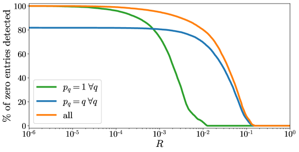
Figure 1: Percentage of zero entries in ${\mathbf{{x}}}^{\star}$ detected by the safe screening tests as a function of $R$, the radius of the safe sphere. Each curve corresponds to a different implementation of the safe screening test (25): $p_{q}=1$ $\forall q$, see (27) (green curve), $p_{q}=q$ $\forall q$, see (29) (blue curve), and all possible choices for $\{p_{q}\}_{q\in\llbracket{1,{n}\rrbracket}}$ (orange curve). The results are generated by using the OSCAR-1 sequence for $\{{\gamma}_{k}\}_{k=1}^{n}$, the Toeplitz dictionary and the ratio $\lambda/\lambda_{\max}=0.5$, see Section 5.1.

In practice, we may expect this conclusion to remain valid when $R$ is “sufficiently” close to zero. This behavior is illustrated in Figure 1. The figure represents the proportion of zeros entries of ${\mathbf{{x}}}^{\star}$ detected by screening test (25) for different “qualities” of the safe region and different choices of parameters $\{p_{q}\}_{q\in\llbracket{1,{n}\rrbracket}}$. We refer the reader to Section 5.1 for a detailed description of the simulation setup. The center of the safe sphere used to apply (25) is assumed to be equal (up to machine precision) to ${{\mathbf{{u}}}^{\star}}$ and the $x$-axis of the figure represents the radius $R$ of the sphere region. The green curve corresponds to test (27); the orange curve represents the screening performance achieved when test (25) is implemented for all possible choices for $\{p_{q}\}_{q\in\llbracket{1,{n}\rrbracket}}$. We note that, as expected, the green curve attains the best screening performance as soon as $R$ becomes close to zero.

At the other extreme of the spectrum, another case of interest reads as:

(28) $$\forall q\in\llbracket{1,{n}\rrbracket}:\ p_{q}=q.$$

Using our initial hypothesis (3), the screening test (25) rewrites

(29) $$|{{\mathbf{a}}^{\operatorname{T}}_{\ell}\mathbf{c}}|<\lambda{\gamma}_{n}-R\implies{\mathbf{{x}}}^{\star}_{(\ell)}=0.$$

Interestingly, this test has the same mathematical structure as (14) with the exception that $\lambda$ is multiplied by the value of the smallest weighting coefficient ${\gamma}_{n}$. In particular, if ${\gamma}_{k}=1$ $\forall k\in\llbracket{1,{n}\rrbracket}$ SLOPE reduces to LASSO and test (29) is equivalent to (14); Theorem 4.3 thus encompasses standard screening rule (14) for LASSO as a particular case. The following result emphasizes that (29) is in fact the best screening rule within the family of tests defined by Theorem 4.3 when ${\gamma}_{k}=1$ $\forall k\in\llbracket{1,{n}\rrbracket}$:

Lemma 4.4.

If ${\gamma}_{k}=1$ $\forall k\in\llbracket{1,{n}\rrbracket}$ and test (25) passes for some choice of parameters $\{p_{q}\}_{q\in\llbracket{1,{n}\rrbracket}}$, then test (29) also succeeds.

A proof of this result is available in Section B.3.

As a final remark, let us mention that, although we just emphasized that some choices of parameters $\{p_{q}\}_{q\in\llbracket{1,{n}\rrbracket}}$ can be optimal (in terms of screening performance) in some situations, no conclusion can be drawn in the general case. In particular, we found in our numerical experiments that the best choice for $\{p_{q}\}_{q\in\llbracket{1,{n}\rrbracket}}$ depends on many factors: the weights $\{{\gamma}_{k}\}_{k=1}^{n}$, the radius of the safe sphere $R$, the nature of the dictionary, the atom to screen, etc. This is illustrated in Fig. 1: we see that the blue and green curves deviate from the orange curve for certain values of $R$, that is the best screening performance is not necessarily achieved for $p_{q}=1$ or $p_{q}=q\ \forall q\in\llbracket{1,{n}\rrbracket}$.

4.3 Efficient implementation

Since the best values for $\{p_{q}\}_{q\in\llbracket{1,{n}\rrbracket}}$ cannot be foreseen, it is desirable to evaluate the screening rule (25) for any choice of these parameters. Formally, this ideal test reads:

(30) $$\forall q\in\llbracket{1,{n}\rrbracket},\exists p_{{q}}\in\llbracket{1,q\rrbracket}:\big{|}{\mathbf{a}}^{\operatorname{T}}_{\ell}\mathbf{c}\big{|}+\sum_{k=p_{{q}}}^{q-1}\big{|}{\mathbf{A}}^{\operatorname{T}}_{\backslash\ell}\mathbf{c}\big{|}_{[k]}<\kappa_{q,p_{{q}}}\implies{\mathbf{{x}}}^{\star}_{(\ell)}=0.$$

Since verifying this test for a given index $\ell$ involves the evaluation of $\mathcal{O}({n}^{2})$ inequalities, a brute-force evaluation of (30) for all atoms of the dictionary requires $\mathcal{O}({n}^{3})$ operations. In this section, we present a procedure to perform this task with a complexity scaling as $\mathcal{O}({n}\log{n}+TL)$ where $T\leq{n}$ is some problem-dependent constant (to be defined later on) and $L$ is the number of atoms of the dictionary passing test (30). Our procedure is summarized in Algorithms 1 and 2, and is grounded on the following nesting properties.

Algorithm 1 Fast implementation of SLOPE screening test (30)

0:  radius $R\geq 0$, sorted elements $\{|{\mathbf{A}}^{\operatorname{T}}\mathbf{c}|_{[k]}\}_{k=1}^{n}$

1:  $\mathcal{L}=\emptyset$ {Set of screened atoms: init}

2:  $\ell={n}$ {Index of atom under testing: init}

3:  Evaluate $\{g({p})\}_{{p}=1}^{{n}}$, $\{p^{\star}({q})\}_{{q}=1}^{{n}}$, $\{q^{\star}(k)\}_{k=1}^{{n}}$

4:  $\mathrm{run}=1$

5:  while $\mathrm{run}==1$ and $\ell>0$ do

6:     $\mathrm{test}$ = Algorithm 2($R$,$\ell$,$\{g({p})\}_{{p}=1}^{{n}}$,$\{p^{\star}({q})\}_{{q}=1}^{{n}}$,$\{q^{\star}(k)\}_{k=1}^{{n}}$)

7:     if $\mathrm{test}==1$ then

8:        $\mathcal{L}=\mathcal{L}\cup\{\ell\}$

9:        $\ell=\ell-1$

10:     else

11:        $\mathrm{run}=0$ {Stop testing as soon as one atom does not pass the test}

12:     end if

13:  end while

14:  return  $\mathcal{L}$ (Set of indices passing test (30))

Nesting of the tests for different atoms

We first emphasize that there exists an implication between the failures of test (30) for some group of indices. In particular, the following result holds:

Lemma 4.5.

Let $B_{q,\ell}$ be defined as in Lemma 4.2 and assume that

(31) $$\left|{{\mathbf{a}}^{\operatorname{T}}_{1}\mathbf{c}}\right|\geq\ldots\geq\left|{{\mathbf{a}}^{\operatorname{T}}_{{n}}\mathbf{c}}\right|.$$

Then $\forall q\in\llbracket{1,{n}\rrbracket}$:

(32) $$\ell<\ell^{\prime}\implies B_{q,\ell}\geq B_{q,\ell^{\prime}}.$$

A proof of this result is provided in Section B.4. Lemma 4.5 has the following consequence: if (31) holds, the failure of test (30) for some $\ell^{\prime}\in\llbracket{2,{n}\rrbracket}$ implies the failure of the test for any index $\ell\in\llbracket{1,\ell^{\prime}-1\rrbracket}$. This immediately suggests a backward strategy for the evaluation of (30), starting from $\ell={n}$ and going backward to smaller indices. This is the sense of the main recursion in Algorithm 1.

We note that hypothesis (31) can always be verified by a proper reordering of the elements of $|{\mathbf{A}}^{\operatorname{T}}\mathbf{c}$|. This can be achieved by state-of-the-art sorting procedures with a complexity of $\mathcal{O}({n}\log{n})$. Therefore, in the sequel we will assume that (31) holds even if not explicitly mentioned.

Nesting of some inequalities

We next show that the number of inequalities to be verified may possibly be substantially smaller than $\mathcal{O}({n}^{2})$. We first focus on the case “$\ell={n}$” and then extend our result to the general case “$\ell<{n}$”.

Let us first note that under hypothesis (31):

(33) $$\forall k\in\llbracket{1,{n}-1\rrbracket}:\ |{\mathbf{A}}^{\operatorname{T}}_{\backslash{n}}\mathbf{c}|_{[k]}=|{\mathbf{A}}^{\operatorname{T}}_{\backslash{n}}\mathbf{c}|_{(k)},$$

that is the $k$th largest element of $|{\mathbf{A}}^{\operatorname{T}}_{\backslash{n}}\mathbf{c}|$ is simply equal to its $k$th component. The particularization of (30) to $\ell={n}$ can then be rewritten as:

(34) $$\forall q\in\llbracket{1,{n}\rrbracket},\exists p_{q}\in\llbracket{1,q\rrbracket}:\ \left|{{\mathbf{a}}^{\operatorname{T}}_{{n}}\mathbf{c}}\right|<\tau_{q,p_{q}}$$

where $\tau_{q,p}$ is defined $\forall q\in\llbracket{1,{n}\rrbracket}$ and $p\in\llbracket{1,q\rrbracket}$ as

(35) $$\tau_{q,p}\triangleq\kappa_{q,p}-\sum_{k=p}^{q-1}\left|{{\mathbf{A}}^{\operatorname{T}}\mathbf{c}}\right|_{(k)}=\sum_{k=p}^{q-1}(\lambda{\gamma}_{k}-\left|{{\mathbf{A}}^{\operatorname{T}}\mathbf{c}}\right|_{(k)}-R)+(\lambda{\gamma}_{q}-R).$$

We show hereafter that (34) can be verified by only considering a “well-chosen” subset of thresholds $\mathcal{T}\subseteq\left\{{{\tau_{q,p}}\colon{q\in\llbracket{1,{n}\rrbracket},p\in\llbracket{1,q\rrbracket}}}\right\}$, see Lemma 4.6 below.

If

(36) $$p^{\star}(q)\triangleq\operatornamewithlimits{arg\,max}_{p\in\llbracket{1,q\rrbracket}}\tau_{q,p},$$

we obviously have

(37) $$\left|{{\mathbf{a}}^{\operatorname{T}}_{{n}}\mathbf{c}}\right|<\tau_{q,p^{\star}(q)}\iff\exists p_{{q}}\in\llbracket{1,q\rrbracket}:\ \left|{{\mathbf{a}}^{\operatorname{T}}_{{n}}\mathbf{c}}\right|<\tau_{q,p_{{q}}}.$$

In other words, for each $q\in\llbracket{1,{n}\rrbracket}$, satisfying the inequality “$\left|{{\mathbf{a}}^{\operatorname{T}}_{{n}}\mathbf{c}}\right|<\tau_{q,p}$” for $p=p^{\star}(q)$ is necessary and sufficient to ensure that it is verified for some $p_{{q}}\in\llbracket{1,q\rrbracket}$. Motivated by this observation, we show the following items below: i) $p^{\star}(q)$ can be evaluated $\forall q\in\llbracket{1,{n}\rrbracket}$ with a complexity $\mathcal{O}({n})$; ii) similarly to $p$, only a subset of values of $q\in\llbracket{1,{n}\rrbracket}$ are of interest to implement (34).

Let us define the function:

(38) $$\begin{array}[b]{@{\,}r@{}r@{}c@{}l@{\,}}{g}\colon{}&{\llbracket{1,{n}\rrbracket}}&{}\to{}&{\mathbb{R}}\\ &{p}&{}\mapsto{}&{\sum_{k=p}^{{n}}(\lambda{\gamma}_{k}-\left|{{\mathbf{A}}^{\operatorname{T}}\mathbf{c}}\right|_{(k)}-R)}\end{array}.$$

We then have $\forall q\in\llbracket{1,{n}\rrbracket}$ and $p\in\llbracket{1,q\rrbracket}$:

(39) $$\tau_{q,p}=g(p)-(g(q)-\lambda{\gamma}_{q})-R.$$

In view of (39), the optimal value $p^{\star}(q)$ can be computed as

(40) $$p^{\star}(q)=\operatornamewithlimits{arg\,max}_{p\in\llbracket{1,q\rrbracket}}g(p).$$

Considering (38), we see that the evaluation of $g(p)$ $\forall p\in\llbracket{1,{n}\rrbracket}$ (and therefore $p^{\star}(q)$ $\forall q\in\llbracket{1,{n}\rrbracket}$) can be done with a complexity scaling as $\mathcal{O}({n})$. This proves item i).

Let us now show that only some specific indices $q\in\llbracket{1,{n}\rrbracket}$ are of interest to implement (34). Let

(41) $$q^{\star}(k)\triangleq\operatornamewithlimits{arg\,max}_{q\in\llbracket{1,k\rrbracket}}g(q)-\lambda{\gamma}_{q},$$

and define the sequence $\{q^{(t)}\}_{t}$ as

(42) $$\begin{cases}q^{(1)}&=q^{\star}({n})\\ q^{(t)}&=q^{\star}(p^{\star}(q^{(t-1)})-1)\end{cases}$$

where the recursion is applied as long as $p^{\star}(q^{(t-1)})>1$. We then have the following result whose proof is available in Section B.5:

Lemma 4.6.

Let $\mathcal{T}\triangleq\left\{{{\tau_{q,p^{\star}(q)}}\colon{q\in\{q^{(t)}\}_{t}}}\right\}$ where $\{q^{(t)}\}_{t}$ is defined in (42). Test (34) is passed if and only if

(43) $$\forall\tau\in\mathcal{T}:\ |{\mathbf{a}}^{\operatorname{T}}_{{n}}\mathbf{c}|<\tau.$$

Lemma 4.6 suggests the procedure described in Algorithm 2 (with $\ell={n}$) to verify if (34) is passed. In a nutshell, the lemma states that only $\mathrm{card}(\mathcal{T})$ inequalities need to be taken into account to implement (34). We note that $\mathrm{card}(\mathcal{T})\leq{n}$ since only one value of $p$ (that is $p^{\star}(q)$) has to be considered for any $q\in\llbracket{1,{n}\rrbracket}$. This is in contrast with a brute-force evaluation of (34) which requires the verification of $\mathcal{O}({n}^{2})$ inequalities.

Algorithm 2 Check if test (30) is passed for $\ell$ if it is passed for $\ell^{\prime}>\ell$

0:  radius $R\geq 0$, index $\ell\in\llbracket{1,{n}\rrbracket}$, $\{g({p})\}_{{p}=1}^{{n}}$, $\{p^{\star}({q})\}_{{q}=1}^{{n}}$,$\{q^{\star}(k)\}_{k=1}^{{n}}$

1:  $q=q^{\star}(\ell)$

2:  $\mathrm{test}=1$

3:  $\mathrm{run}=1$

4:  while $\mathrm{run}==1$ do

5:     $\tau=g(p^{\star}(q))-g(q)+(\lambda{\gamma}_{q}-R)$ {Evaluation of current threshold, see (39)}

6:     if $|{\mathbf{a}}^{\operatorname{T}}_{\ell}\mathbf{c}|\geq\tau$ then

7:        $\mathrm{test}=0$ {Test failed}

8:        $\mathrm{run}=0$ {Stops the recursion}

9:     end if

10:     if $p^{\star}(q)>1$ then

11:        $q=q^{\star}(p^{\star}(q)-1)$ {Next value of $q$ to test, see (42)}

12:     else

13:        $\mathrm{run}=0$ {Stops the recursion}

14:     end if

15:  end while

16:  return  $\mathrm{test}$ ($=1$ if test passed and $0$ otherwise)

We finally emphasize that the procedure described in Algorithm 2 also applies to $\ell<{n}$ as long as the screening test is passed for all $\ell^{\prime}>\ell$. More specifically, if test (30) is passed for all $\ell^{\prime}\in\llbracket{\ell+1,{n}\rrbracket}$, then its particularization to atom $\mathbf{a}_{\ell}$ reads

(44) $$\forall\tau\in\mathcal{T}^{\prime}:\ \left|{{\mathbf{a}}^{\operatorname{T}}_{\ell}\mathbf{c}}\right|<\tau$$

for some $\mathcal{T}^{\prime}\subseteq\mathcal{T}$.

Indeed, if screening test (30) is passed for all $\ell^{\prime}\in\llbracket{\ell+1,{n}\rrbracket}$, the corresponding elements can be discarded from the dictionary and we obtain a reduced problem only involving atoms $\{\mathbf{a}_{\ell^{\prime}}\}_{\ell^{\prime}\in\llbracket{1,\ell\rrbracket}}$. Since (31) is assumed to hold, $\mathbf{a}_{\ell}$ attains the smallest absolute inner product with $\mathbf{c}$ and we end up with the same setup as in the case “$\ell={n}$”. In particular, if screening test (30) is passed for all $\ell^{\prime}\in\llbracket{\ell+1,{n}\rrbracket}$, Lemma 4.6 still holds for $\mathbf{a}_{\ell}$ by letting $q^{(1)}=q^{\star}(\ell)$ in the definition of the sequence $\{q^{(t)}\}_{t}$ in (42).

To conclude this section, let us summarize the complexity needed to implement Algorithms 1 and 2. First, Algorithm 1 requires the entries $|{\mathbf{A}}^{\operatorname{T}}\mathbf{c}|$ to be sorted to satisfy hypothesis (4.5). This involves a complexity $\mathcal{O}({n}\log{n})$. Moreover, the sequences $\{g({p})\}_{{p}=1}^{{n}}$, $\{p^{\star}({q})\}_{{q}=1}^{{n}}$, $\{q^{\star}(k)\}_{k=1}^{{n}}$ can be evaluated with a complexity $\mathcal{O}({n})$. Finally, the main recursion in Algorithm 1 implies to run Algorithm 2 $L$ times, where $L$ is the number of atoms passing test (30). Since Algorithm 2 requires to verify at most $T=\mathrm{card}\left({\mathcal{T}}\right)$ inequalities, the overall complexity of the main recursion scales as $\mathcal{O}(LT)$. Overall, the complexity of Algorithm 1 is therefore $\mathcal{O}({n}\log{n}+LT)$.

5 Numerical simulations

We present hereafter several simulation results demonstrating the effectiveness of the proposed screening procedure to accelerate the resolution of SLOPE. This section is organized as follows. In Section 5.1, we present the experimental setups considered in our simulations. In Section 5.2 we compare the effectiveness of different screening strategies. In Section 5.3, we show that our methodology enables to reach better convergence properties for a given computational budget.

5.1 Experimental setup

We detail below the experimental setups used in all our numerical experiments.

Dictionaries and observation vectors: New realizations of $\mathbf{A}$ and $\mathbf{y}$ are drawn for each trial as follows. The observation vector is generated according to a uniform distribution on the ${m}$-dimensional sphere. The elements of $\mathbf{A}$ obey one of the following models:

1. the entries are i.i.d. realizations of a centered Gaussian,

2. the entries are i.i.d. realizations of a uniform distribution on $[0,1]$,

3. the columns are shifted versions of a Gaussian curve.

For all distributions, the columns of $\mathbf{A}$ are normalized to have unit $\ell_{2}$-norm. In the following, these three options will be respectively referred to as “Gaussian”, “Uniform” and “Toeplitz”.

Regularization parameters: We consider three different choices for the sequence $\{{\gamma}_{k}\}_{k=1}^{n}$, each of them corresponding to a different instance of the well-known OSCAR problem [7, Eq. (3)]. More specifically, we let

(45) $$\forall k\in\llbracket{1,{n}\rrbracket}:\ {\gamma}_{k}\triangleq\beta_{1}+\beta_{2}({n}-k)$$

where $\beta_{1}$, $\beta_{2}$ are nonnegative parameters chosen so that ${\gamma}_{1}=1$ and ${\gamma}_{n}\in\{.9,.1,10^{-3}\}$. In the sequel, these parametrizations will respectively be referred to as “OSCAR-1”, “OSCAR-2” and “OSCAR-3”.

5.2 Performance of screening strategies

We first compare the effectiveness of different screening strategies described in Section 4. More specifically, we evaluate the proportion of zero entries in ${\mathbf{{x}}}^{\star}$ – the solution of SLOPE problem (1) – that can be identified by tests (27), (29) and (30) as a function of the “quality” of the safe sphere. These tests will respectively be referred to as “test-p=1”, “test-p=q” and “test-all” in the following. Figures 1 (see Section 4.2) and 2 represent this criterion of performance as a function of some parameter $R_{0}$ (described below) and different values of the ratio $\lambda/\lambda_{\max}$. The results are averaged over $50$ realizations. For each simulation trial, we draw a new realization of $\mathbf{y}\in\mathbb{R}^{100}$ and $\mathbf{A}\in\mathbb{R}^{100\times 300}$ according to the distributions described in Section 5.1. We consider Toeplitz dictionaries in Figure 1 and Gaussian dictionaries in Figure 2.

The safe sphere used in the screening tests is constructed as follows. A primal-dual solution $({\mathbf{{x}}}_{a},{\mathbf{{u}}}_{a})$ of problems (1) and (19) is evaluated with “high-accuracy”, i.e., with a duality GAP of $10^{-14}$ as stopping criterion. More precisely, ${\mathbf{{x}}}_{a}$ is first evaluated by solving the SLOPE problem (1) with the algorithm proposed in [5]. To evaluate ${\mathbf{{u}}}_{a}$, we extend the so-called “dual scaling” operator [24, Section 3.3] to the SLOPE problem: we let ${\mathbf{{u}}}_{a}=(\mathbf{y}-\mathbf{A}{\mathbf{{x}}}_{a})/\beta(\mathbf{y}-\mathbf{A}{\mathbf{{x}}}_{a})$ where

(46) $$\forall\mathbf{z}\in\mathbb{R}^{m}:\ \beta(\mathbf{z})\triangleq\max\left({1,\max_{q\in\llbracket{1,{n}\rrbracket}}\frac{\sum_{k=1}^{q}\left|{{\mathbf{A}}^{\operatorname{T}}\mathbf{z}}\right|_{[k]}}{\lambda\sum_{k=1}^{q}{\gamma}_{k}}}\right).$$

The couple $({\mathbf{{x}}}_{a},{\mathbf{{u}}}_{a})$ is then used to construct a sphere $\mathcal{S}(\mathbf{c}_{a},R_{a})$ in $\mathbb{R}^{m}$ whose parameters are given by

(47a) $$\mathbf{c}\;=\; {\mathbf{{u}}}_{a}$$

(47b) $$R\;=\; R_{0}+\sqrt{2\left({{P}({\mathbf{{x}}}_{a})-{D}({\mathbf{{u}}}_{a})}\right)}$$

where $R_{0}$ is a nonnegative scalar. We note that for $R_{0}=0$, the latter sphere corresponds to the GAP safe sphere described in (15). Hence, (47a) and (47b) define a safe sphere for any choice of the nonnegative scalar $R_{0}\geq 0$.

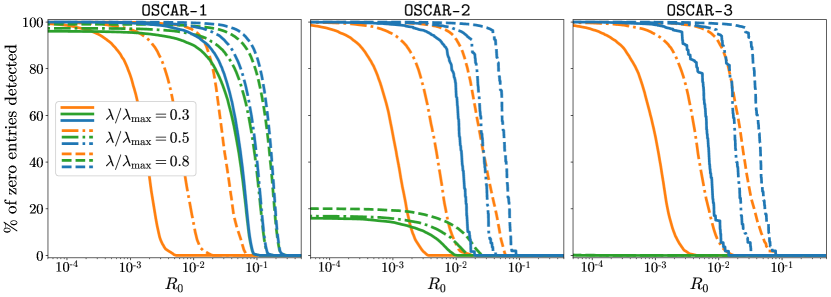
Figure 2: Percentage of zero entries in the solution of the SLOPE problem identified by test-p=1 (orange lines), test-p=q (green lines) and test-all (blue lines) as a function of $R_{0}$ for the Gaussian dictionary, three values of $\lambda/\lambda_{\max}$ and three parameter sequences $\{{\gamma}_{k}\}_{k=1}^{n}$.

Figure 1 concentrates on the sequence OSCAR-1 whereas each subfigure corresponds to a different choice for $\{{\gamma}_{k}\}_{k=1}^{n}$ in Figure 2. For the three considered screening strategies, we observe that the detection performance decreases as $R_{0}$ increases. Interestingly, different behaviors can be noticed. For all simulation setups, test-p=1 reaches a detection rate of $100\%$ whenever $R_{0}$ is sufficiently small. The performance of test-p=q varies from one sequence to another: it outperforms test-p=1 for OSCAR-1, is able to detect at most $20\%$ of the zeros for OSCAR-2 and fail for all values of $R_{0}$ for OSCAR-3. Finally, test-all outperforms quite logically the two other strategies. The gap in performance depends on both the considered setup and the radius $R_{0}$ but can be quite significant in some cases. For example, when $\lambda/\lambda_{\max}=0.5$ and $R_{0}=10^{-2}$, there is $80\%$ more entries passing test-all than test-p=1 for all parameter sequences.

These results may be explained as follows. First, we already mentioned in Section 4 that when the radius of the safe sphere is sufficiently small (that is, when $R_{0}$ is close to zero), test-p=1 is expected to be the best screening test within the family of tests defined in Theorem 4.3. Similarly, if the SLOPE weights satisfy ${\gamma}_{1}={\gamma}_{n}$, we showed in Lemma 4.4 that no test in Theorem 4.3 can outperform test-p=q. Hence, one may reasonably expect that this conclusion remains valid whenever ${\gamma}_{1}\simeq{\gamma}_{n}$, as observed for the sequence OSCAR-1 in our simulations. On the other hand, passing test-p=q becomes more difficult as parameter ${\gamma}_{n}$ is small. As a matter of fact, the test will never pass when ${\gamma}_{n}=0$. In our experiments, the sequences $\{{\gamma}_{k}\}_{k=1}^{n}$ are such that ${\gamma}_{n}$ is close to zero for OSCAR-2 and OSCAR-3. Finally, since test-all encompasses the two other tests, it is expected to always perform at least as well as the latter.

5.3 Benchmarks

As far as our simulation setup is concerned, the results presented in the previous section show a significant advantage in implementing test-all in terms of detection performance. However, this conclusion does not include any consideration about the numerical complexity of the tests. We note that, although the proposed screening rules can lead to a significant reduction of the problem dimensions, our tests also induce some additional computational burden. In particular, we emphasized in Section 4.3 that test-all can be verified for all atoms of the dictionary with a complexity $\mathcal{O}({n}\log{n}+TL)$ where $T\leq{n}$ is a problem-dependent parameter and $L$ is the number of atoms passing the test. Moreover, we also note that, as far as a GAP safe sphere is considered in the implementation of the tests, its construction requires the identification of a dual feasible point ${\mathbf{{u}}}$ and this operation typically induces a computational overhead of $\mathcal{O}({n}\log{n})$ (see below for more details).

In this section, we therefore investigate the benefits (from a “complexity-accuracy trade-off” point of view) of interleaving the proposed safe screening methodology with the iterations of an accelerated proximal gradient algorithm [5]. In all our tests, we consider the GAP safe sphere defined in (15). The primal point used in the construction of the GAP sphere corresponds to the current iterate of the solving procedure, say ${\mathbf{{x}}}^{(t)}$. A dual feasible point ${\mathbf{{u}}}^{(t)}$ is constructed as

(48) $${\mathbf{{u}}}^{(t)}=\frac{\mathbf{y}-\mathbf{A}{\mathbf{{x}}}^{(t)}}{\beta(\mathbf{y}-\mathbf{A}{\mathbf{{x}}}^{(t)})}$$

where $\begin{array}[b]{@{\,}r@{}r@{}c@{}l@{\,}}{\beta}\colon{}&{\mathbb{R}^{m}}&{}\to{}&{\mathbb{R}^{m}}\end{array}$ is either defined as in (46) or as follows:

(49) $$\forall\mathbf{z}\in\mathbb{R}^{m}:\ \beta(\mathbf{z})\triangleq\max\left({1,\displaystyle\max_{k\in\llbracket{1,{n}\rrbracket}}\frac{\big{|}{\mathbf{A}}^{\operatorname{T}}\mathbf{z}\big{|}_{[k]}}{\lambda{\gamma}_{k}}}\right).$$

(46) matches the standard definition of the “dual scaling” operator proposed in [24, Section 3.3] whereas (49) corresponds to the option considered in [3]. We notice that the two options require to sort the elements of $\left|{{\mathbf{A}}^{\operatorname{T}}\mathbf{z}}\right|$ and thus lead to a complexity overhead scaling as $\mathcal{O}({n}\log{n})$.

In our simulations, we consider the four following solving strategies:

1. Run the proximal gradient procedure [5] with no screening.

2. Interleave some iterations of the proximal gradient algorithm with test-p=q and construct the dual feasible point with (46).

3. Interleave some iterations of the proximal gradient algorithm with test-p=q and construct the dual feasible point with (49).

4. Interleave some iterations of the proximal gradient algorithm with test-all and construct the dual feasible point with (46).

These strategies will respectively be denoted “PG-no”, “PG-p=q”, “PG-Bao” and “PG-all” in the sequel. We note that PG-Bao closely matches the solving procedure considered in [3].

We compare the performance of these solving strategies by resorting to Dolan-Moré profiles [15]. More precisely, we run each procedure for a given budget of time (that is the algorithm is stopped after a predefined amount of time) on $I=50$ different instances of the SLOPE problems. In PG-p=q, PG-Bao and PG-all, the screening procedure is applied once every 20 iterations. Each problem instance is generated by drawing a new dictionary $\mathbf{A}\in\mathbb{R}^{100\times 300}$ and observation vector $\mathbf{y}\in\mathbb{R}^{100}$ according to the distributions described in Section 5.1. We then compute the following performance profile for each solver $\texttt{solv}\in\left\{{\text{{PG-no}{}, {PG-p=q}{}, {PG-Bao}{}, {PG-all}{}}}\right\}$:

(50) $$\rho_{\texttt{solv}}(\delta)\triangleq 100\,\frac{\mathrm{card}\left({\left\{{{i\in\llbracket{1,I\rrbracket}}\colon{d_{i,\texttt{solv}}\leq\delta}}\right\}}\right)}{I}\quad\forall\delta\in\mathbb{R}_{+}$$

where $d_{i,\texttt{solv}}$ denotes the dual gap attained by solver solv for problem instance $i$. $\rho_{\texttt{solv}}(\delta)$ thus represents the (empirical) probability that solver solv reaches a dual gap no greater than $\delta$ for the considered budget of time.

Figure 3 presents the performance profiles obtained for three types of dictionaries (Gaussian, Uniform and Toeplitz) and three different weighting sequences $\{{\gamma}_{k}\}_{k=1}^{n}$ (OSCAR-1, OSCAR-2 and OSCAR-3). The results are displayed for $\lambda/\lambda_{\max}=0.5$ but similar performance profiles have been obtained for other values of the ratio $\lambda/\lambda_{\max}$. All algorithms are implemented in Python with Cython bindings and experiments are run on a Dell laptop, 1.80 GHz, Intel Core i7. For each setup, we adjusted the time budget so that $\rho_{\text{{PG-all}{}}}(10^{-8})\simeq 50\%$ for the sake of comparison.

As far as our simulation setup is concerned, these results show that the proposed screening methodologies improve the solving accuracy as compared to a standard proximal gradient. PG-all improves the average accuracy over PG-no in all the considered settings. The gap in performance depends on the setup but is generally quite significant. PG-p=q also enhances the average accuracy in most cases and performs at least comparably to PG-Bao in all setups. As expected, the behavior of PG-p=q and PG-Bao is more sensitive to the choice of the weighting sequence $\{{\gamma}_{k}\}_{k=1}^{n}$. In particular, the screening performance of these strategies decreases when ${\gamma}_{n}\simeq 0$ as emphasized in Section 5.2. This results in no accuracy gain over PG-no for the sequence OSCAR-3 as illustrated in Figure 3. Nevertheless, we note that, even in absence of gain, PG-p=q and PG-Bao do not seem to significantly degrade the performance as compared to PG-no.

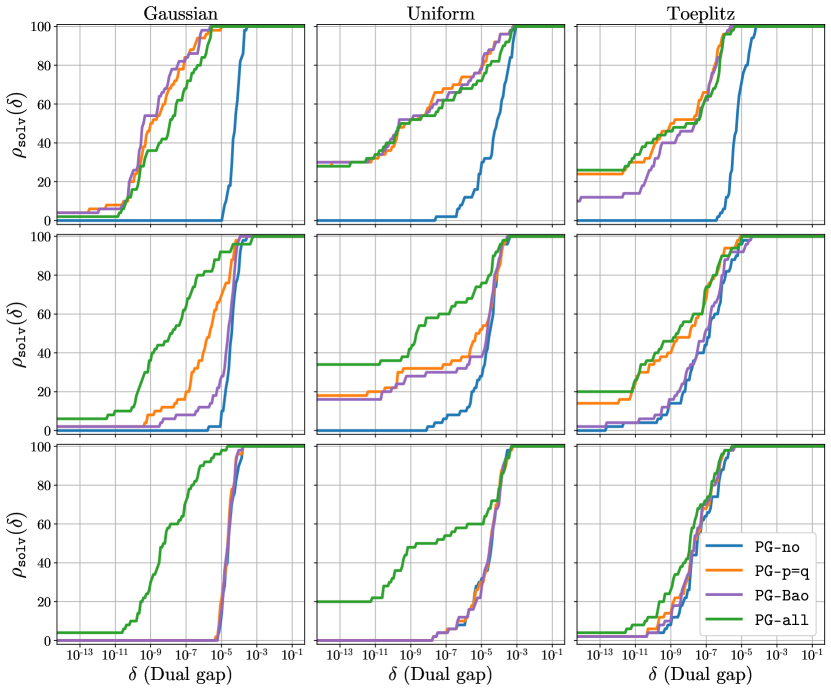
Figure 3: Performance profiles of PG-no, PG-p=q, PG-Bao and PG-all obtained for the “Gaussian” (column 1), “Uniform” (column 2) and “Toeplitz” (column 3) dictionaries and $\lambda/\lambda_{\max}=0.5$ with a budget of time. First row: OSCAR-1, second row: OSCAR-2 and third row: OSCAR-3.

6 Conclusions

In this paper we proposed a new methodology to safely identify the zeros of the solutions of the SLOPE problem. In particular, we introduced a family of screening rules indexed by some parameters $\{p_{q}\}_{q=1}^{n}$ where ${n}$ is the dimension of the primal variable. Each test of this family takes the form of a series of ${n}$ inequalities which, when verified, imply the nullity of some coefficient of the minimizers. Interestingly, the proposed tests encompass standard “sphere” screening rule for LASSO as a particular case for some $\{p_{q}\}_{q=1}^{n}$, although this choice does not correspond to the most effective test in the general case. We then introduced an efficient numerical procedure to jointly evaluate all the tests in the proposed family. Our algorithm has a complexity $\mathcal{O}({n}\log{n}+TL)$ where $T\leq{n}$ is some problem-dependent constant and $L$ is the number of elements passing at least one test of the family. We finally assessed the performance of our screening strategy through numerical simulations and showed that the proposed methodology leads to significant improvements of the solving accuracy for a prescribed computational budget.

Appendix A Miscellaneous results

Section A.1 reminds some useful results from convex analysis applied to the SLOPE problem (1). Section A.2 provides a proof of (17). In all the statements below, $\partial{{r}}_{\textnormal{slope}}({\mathbf{{x}}})$ denotes the subdifferential of ${{r}}_{\textnormal{slope}}$ evaluated at ${\mathbf{{x}}}$.

A.1 Some results of convex analysis

We remind below several results of convex analysis that will be used in our subsequent derivations. The first lemma provides a necessary and sufficient condition for ${\mathbf{{x}}}^{\star}\in\mathbb{R}^{n}$ to be a minimizer of the SLOPE problem (1):

Lemma A.1.

$\text{${\mathbf{{x}}}^{\star}$ is a minimizer of~{}\eqref{eq:primal problem}}\ \Longleftrightarrow\ {\lambda}^{-1}{\mathbf{A}}^{\operatorname{T}}(\mathbf{y}-\mathbf{A}{\mathbf{{x}}}^{\star})\in\partial{{r}}_{\textnormal{slope}}({\mathbf{{x}}}^{\star})$.

Lemma A.1 follows from a direct application of Fermat’s rule [4, Proposition 16.4] to problem (1). We note that under condition (3), ${{r}}_{\textnormal{slope}}$ defines a norm on $\mathbb{R}^{n}$, see e.g., [6, Proposition 1.1] or [48, Lemma 2]. The subdifferential $\partial{{r}}_{\textnormal{slope}}({\mathbf{x}})$ is therefore well defined for all ${\mathbf{x}}\in\mathbb{R}^{n}$ and writes as

(51) $$\partial{{r}}_{\textnormal{slope}}({\mathbf{x}})=\left\{{{\mathbf{g}\in\mathbb{R}^{n}}\colon{{\mathbf{g}}^{\operatorname{T}}{\mathbf{x}}={{r}}_{\textnormal{slope}}({\mathbf{x}})\text{ and }{{r}}_{\textnormal{slope},*}(\mathbf{g})\leq 1}}\right\},$$

where

(52) $${{r}}_{\textnormal{slope},*}(\mathbf{g})\triangleq\sup_{{\mathbf{x}}\in\mathbb{R}^{n}}{\mathbf{g}}^{\operatorname{T}}{\mathbf{{x}}}\ \text{ s.t.}\ {{r}}_{\textnormal{slope}}({\mathbf{x}})\leq 1$$

is the dual norm of ${{r}}_{\textnormal{slope}}$, see e.g., [1, Eq. (1.4)].

The next lemma states a technical result which will be useful in the proof of Theorem 4.1 in Appendix B:

Lemma A.2.

If $\mathbf{g}\in\partial{{r}}_{\textnormal{slope}}({\mathbf{{x}}})$, then ${{\mathbf{{x}}}}^{\operatorname{T}}(\mathbf{g}-\mathbf{g}^{\prime})\geq 0\,\forall\mathbf{g}^{\prime}\in\mathbb{R}^{n}\text{ s.t. }{{r}}_{\textnormal{slope},*}(\mathbf{g}^{\prime})\leq 1.$

Proof A.3.

Let $\mathbf{g}\in\partial{{r}}_{\textnormal{slope}}({\mathbf{{x}}})$. One has

$$\mathbf{g}\in\partial{{r}}_{\textnormal{slope}}({\mathbf{{x}}})\;\Longleftrightarrow\; {\mathbf{{x}}}\in\partial{{r}}_{\textnormal{slope}}^{*}(\mathbf{g})$$

(53) $$\;\Longleftrightarrow\; \forall\mathbf{g}^{\prime}\in\mathbb{R}^{n},\;{{r}}_{\textnormal{slope}}^{*}(\mathbf{g}^{\prime})\geq{{r}}_{\textnormal{slope}}^{*}(\mathbf{g})+\left\langle{{\mathbf{{x}}},\mathbf{g}^{\prime}-\mathbf{g}}\right\rangle$$

where ${{r}}_{\textnormal{slope}}^{*}$ refers to the Fenchel conjugate of ${{r}}_{\textnormal{slope}}$. The first equivalence is a consequence of [4, Theorem 16.29] and the second of the definition of the subdifferential set. Lemma A.2 follows by noticing that ${{r}}_{\textnormal{slope}}^{*}(\mathbf{g}^{\prime})=0$ $\forall\mathbf{g}^{\prime}\in\mathbb{R}^{n}$ such that ${{r}}_{\textnormal{slope},*}(\mathbf{g}^{\prime})\leq 1$ by property of ${{r}}_{\textnormal{slope}}^{*}$ [4, Item (v) of Example 13.3].

In the last lemma of this section, we provide a closed-form expression of the subdifferential and the dual norm of ${{r}}_{\textnormal{slope}}$:

Lemma A.4.

The dual norm and the subdifferential of ${{r}}_{\textnormal{slope}}({\mathbf{{x}}})$ respectively write:

$$\begin{split}{{r}}_{\textnormal{slope},*}(\mathbf{g})&=\max_{q\in\llbracket{1,{n}\rrbracket}}\ \frac{1}{\sum_{k=1}^{q}{\gamma}_{k}}\sum_{k=1}^{q}|\mathbf{g}|_{[k]},\\ \partial{{r}}_{\textnormal{slope}}({\mathbf{x}})&=\left\{{{\mathbf{g}\in\mathbb{R}^{n}}\colon{{\mathbf{g}}^{\operatorname{T}}{\mathbf{x}}={{r}}_{\textnormal{slope}}({\mathbf{x}})\text{ and }\forall q\in\llbracket{1,{n}\rrbracket}:\ \sum_{k=1}^{q}|\mathbf{g}|_{[k]}\leq\sum_{k=1}^{q}{\gamma}_{k}}}\right\}.\end{split}$$

Proof A.5.

The expression of the dual norm is a direct consequence of [48, Lemma 4]. More precisely, the authors showed that

(54) $${{r}}_{\textnormal{slope},*}(\mathbf{g})=\max_{\mathbf{v}\in\bigcup_{q=1}^{n}\mathcal{V}_{q}}\;{\mathbf{g}}^{\operatorname{T}}\mathbf{v}$$

where $\mathcal{V}_{q}\triangleq\left\{{{\tfrac{1}{\sum_{k=1}^{q}{\gamma}_{k}}\mathbf{s}}\colon{\mathbf{s}\in\{0,-1,+1\}^{n},\mathrm{card}\left({\{j:\mathbf{s}_{(j)}\neq 0\}}\right)=q}}\right\}$ for all $q\in\llbracket{1,{n}\rrbracket}$. The expression of ${{r}}_{\textnormal{slope},*}$ given in Lemma A.4 is a compact rewriting of (54) that can be obtained as follows. See first that for all $q\in\llbracket{1,{n}\rrbracket}$,

(55) $$\max_{\mathbf{v}\in\mathcal{V}_{q}}\;{\mathbf{g}}^{\operatorname{T}}\mathbf{v}\leq\frac{1}{\sum_{k=1}^{q}{\gamma}_{k}}\sum_{k=1}^{q}\left|{\mathbf{g}}\right|_{[k]}.$$

Second, for $q\in\llbracket{1,{n}\rrbracket}$, let $\mathcal{J}_{q}\subset\llbracket{1,{n}\rrbracket}$ be a set $q$ distinct indices such that $|\mathbf{g}_{(j)}|\geq\left|{\mathbf{g}}\right|_{[q]}$ for all $j\in\mathcal{J}_{q}$. Then, the upper bound in (55) is attained by evaluating the left-hand side at $\mathbf{v}\in\mathcal{V}_{q}$ defined as

(56) $$\forall j\in\llbracket{1,{n}\rrbracket}:\quad\mathbf{v}_{(j)}=\begin{cases}\tfrac{1}{\sum_{k=1}^{q}{\gamma}_{k}}\,\mathrm{sign}\left({\mathbf{g}_{(j)}}\right)&\text{ if }j\in\mathcal{J}_{q}\\ 0&\text{otherwise.}\end{cases}$$

The expression of the subdifferential follows from (51) by plugging the expression of the dual norm in the inequality “${{r}}_{\textnormal{slope},*}(\mathbf{g})\leq 1$”.

A.2 Proof of (17)

We first observe that

(57) $$\text{${\mathbf{0}}_{n}$ is not a minimizer of~{}\eqref{eq:primal problem}}\Longleftrightarrow{\lambda}^{-1}{\mathbf{A}}^{\operatorname{T}}\mathbf{y}\notin\partial{{r}}_{\textnormal{slope}}({\mathbf{0}}_{n}),$$

as a direct consequence of Lemma A.1. Particularizing the expression of $\partial{{r}}_{\textnormal{slope}}({\mathbf{x}})$ in Lemma A.4 to ${\mathbf{x}}={\bf 0}_{n}$, the right-hand side of (57) can equivalently be rewritten as

(58) $$\exists q\in\llbracket{1,{n}\rrbracket}:\;{\lambda}^{-1}\sum_{k=1}^{q}\big{|}{{\mathbf{A}}^{\operatorname{T}}\mathbf{y}}\big{|}_{[k]}>\sum_{k=1}^{q}{\gamma}_{k}.$$

Since ${\gamma}_{1}>0$ and the sequence $\{{\gamma}_{k}\}_{k=1}^{{n}}$ is nonnegative by hypothesis (3), (58) can also be rewritten as

(59) $$\exists q\in\llbracket{1,{n}\rrbracket}:\;\lambda<\frac{\sum_{k=1}^{q}\big{|}{{\mathbf{A}}^{\operatorname{T}}\mathbf{y}}\big{|}_{[k]}}{\sum_{k=1}^{q}{\gamma}_{k}}.$$

The statement in (17) then follows by noticing that the right-hand side of (16) is a compact reformulation of (59).

Appendix B Proofs related to screening tests

B.1 Proof of Theorem 4.1

In this section, we provide the technical details leading to (21). Our derivation leverages the Fermat’s rule and the expression of the subdifferential derived in Lemma A.4.

We prove (21) by contraposition. More precisely, we show that if ${\mathbf{{x}}}^{\star}_{(\ell)}\neq 0$ for some $\ell\in\llbracket{1,{n}\rrbracket}$, then

(60) $$\exists q_{0}\in\llbracket{1,{n}\rrbracket},\;\big{|}{\mathbf{a}}^{\operatorname{T}}_{\ell}{{\mathbf{{u}}}^{\star}}\big{|}+\sum_{k=1}^{q_{0}-1}\big{|}{\mathbf{A}}^{\operatorname{T}}_{\backslash\ell}{{\mathbf{{u}}}^{\star}}\big{|}_{[k]}=\lambda\sum_{k=1}^{q_{0}}{\gamma}_{k}.$$

Using Lemma A.1 and the following connection between primal-dual solutions (see [6, Section 2.5])

(61) $${{\mathbf{{u}}}^{\star}}=\mathbf{y}-\mathbf{A}{\mathbf{{x}}}^{\star},$$

we have that ${\mathbf{{x}}}^{\star}$ is a minimizer of (1) if and only if

(62) $$\mathbf{g}^{\star}\triangleq{\lambda}^{-1}{\mathbf{A}}^{\operatorname{T}}{{\mathbf{{u}}}^{\star}}\in\partial{{r}}_{\textnormal{slope}}({\mathbf{{x}}}^{\star}).$$

In the rest of the proof, we will use Lemma A.2 with ${\mathbf{x}}={\mathbf{{x}}}^{\star}$, $\mathbf{g}=\mathbf{g}^{\star}$ and different instances of vector $\mathbf{g}^{\prime}$ to prove our statement. First, let us define $\mathbf{g}^{\prime}\in\mathbb{R}^{n}$ as

$$\begin{split}\mathbf{g}^{\prime}_{(j)}\;=\;&\mathbf{g}^{\star}_{(j)}\quad\forall j\in\llbracket{1,{n}\rrbracket}\setminus\{\ell\},\\ \mathbf{g}^{\prime}_{(\ell)}\;=\;&0.\end{split}$$

It is easy to verify that ${{r}}_{\textnormal{slope},*}(\mathbf{g}^{\prime})\leq 1$. Applying Lemma A.2 then leads to

(63) $$\mathbf{g}^{\star}_{(\ell)}{\mathbf{{x}}}^{\star}_{(\ell)}\geq 0.$$

Since ${\mathbf{{x}}}^{\star}_{(\ell)}$ is assumed to be nonzero, we then have

(64) $$\mathrm{sign}\big{(}\mathbf{g}^{\star}_{(\ell)}\big{)}\,\mathrm{sign}\big{(}{\mathbf{{x}}}^{\star}_{(\ell)}\big{)}\geq 0,$$

where the equality holds if and only if $\mathbf{g}^{\star}_{(\ell)}=0$.

Second, let us consider the following choice for $\mathbf{g}^{\prime}\in\mathbb{R}^{n}$:

(65) $$\begin{split}\mathbf{g}^{\prime}_{(j)}\;=\;&\mathbf{g}^{\star}_{(j)}\quad\forall j\in\llbracket{1,{n}\rrbracket}\setminus\{\ell\},\\ \mathbf{g}^{\prime}_{(\ell)}\;=\;&\mathbf{g}^{\star}_{(\ell)}+s\delta,\end{split}$$

where

(66) $$s\triangleq\begin{cases}\mathrm{sign}\big{(}\mathbf{g}^{\star}_{(\ell)}\big{)}&\text{ if }\mathbf{g}^{\star}_{(\ell)}\neq 0\\ \mathrm{sign}\big{(}{\mathbf{{x}}}^{\star}_{(\ell)}\big{)}&\text{ otherwise,}\end{cases}$$

and $\delta$ is any nonnegative scalar such that

(67) $${{r}}_{\textnormal{slope},*}(\mathbf{g}^{\prime})\leq 1.$$

On the one hand, we note that (67) is verified for $\delta=0$. On the other hand, it can be seen that (67) is violated as soon as $\delta>0$ by using the following arguments. First, applying Lemma A.2 with $\mathbf{g}^{\prime}$ defined as in (65) leads to

(68) $$-s{\mathbf{{x}}}^{\star}_{(\ell)}\delta\geq 0.$$

Second, using (64) and the definition of $s$ in (66), we must have $s{\mathbf{{x}}}^{\star}_{(\ell)}>0$. Hence, satisfying inequality (67) necessarily implies that $\delta=0$. The contraposition of this result implies:

(69) $$\forall\delta>0,\exists q_{0}\in\llbracket{1,{n}\rrbracket}:\;\sum_{k=1}^{q_{0}}|\mathbf{g}^{\star}|_{[k]}+\delta>\sum_{k=1}^{q_{0}}{\gamma}_{k}$$

or equivalently

(70) $$\exists q_{0}\in\llbracket{1,{n}\rrbracket}:\;\sum_{k=1}^{q_{0}}|\mathbf{g}^{\star}|_{[k]}=\sum_{k=1}^{q_{0}}{\gamma}_{k}.$$

Let us next emphasize that the range of values for $q_{0}$ can be restricted by choosing some suitable value for $\delta$. In particular, define $q_{0}^{\prime}\in\llbracket{1,{n}\rrbracket}$ as

(71) $$q_{0}^{\prime}\triangleq\min\left\{{{q\in\llbracket{1,{n}\rrbracket}}\colon{|\mathbf{g}^{\star}_{(\ell)}|=|\mathbf{g}^{\star}|_{[q]}}}\right\}$$

and let

(72) $$0<\delta<|\mathbf{g}^{\star}|_{[q_{0}^{\prime}-1]}-|\mathbf{g}^{\star}|_{[q_{0}^{\prime}]}$$

with the convention $\mathbf{g}^{\star}_{[0]}=+\infty$. Considering $\mathbf{g}^{\prime}$ as defined in (65) with $\delta$ satisfying (72), we have that the first $q_{0}^{\prime}-1$ largest absolute elements of $\mathbf{g}^{\prime}$ and $\mathbf{g}^{\star}$ are the same. Since ${{r}}_{\textnormal{slope},*}(\mathbf{g}^{\star})\leq 1$, the inequality in the right-hand side of (69) can therefore not be verified for $q_{0}\in\llbracket{1,q_{0}^{\prime}-1\rrbracket}$. Hence, considering $\delta$ as in (72), we have

(73) $$\exists q_{0}\in\llbracket{q_{0}^{\prime},{n}\rrbracket}:\;\sum_{k=1}^{q_{0}}|\mathbf{g}^{\star}|_{[k]}=\sum_{k=1}^{q_{0}}{\gamma}_{k}.$$

We finally obtain our original assertion (60) by using the definition of $\mathbf{g}^{\star}$ in (62) and the fact that

(74) $$\sum_{k=1}^{q_{0}}\big{|}{\mathbf{A}}^{\operatorname{T}}{{\mathbf{{u}}}^{\star}}\big{|}_{[k]}=\big{|}{\mathbf{a}}^{\operatorname{T}}_{\ell}{{\mathbf{{u}}}^{\star}}\big{|}+\sum_{k=1}^{q_{0}-1}\big{|}{\mathbf{A}}^{\operatorname{T}}_{\backslash\ell}{{\mathbf{{u}}}^{\star}}\big{|}_{[k]}$$

since $|{\mathbf{a}}^{\operatorname{T}}_{\ell}{{\mathbf{{u}}}^{\star}}|=|{\mathbf{A}}^{\operatorname{T}}{{\mathbf{{u}}}^{\star}}|_{[q_{0}^{\prime}]}$ by definition of $q_{0}^{\prime}$ in (71) and $|{\mathbf{A}}^{\operatorname{T}}{{\mathbf{{u}}}^{\star}}|_{[q_{0}^{\prime}]}\geq|{\mathbf{A}}^{\operatorname{T}}{{\mathbf{{u}}}^{\star}}|_{[q_{0}]}$ by definition of $q_{0}\geq q_{0}^{\prime}$.

B.2 Proof of Lemma 4.2

We first state and prove the following technical lemma:

Lemma B.1.

Let $\mathbf{g}\in\mathbb{R}^{n}$ and $\mathbf{h}\in\mathbb{R}^{n}$ be such that $\mathbf{g}_{(j)}\leq\mathbf{h}_{(j)}$$\,\forall j\in\llbracket{1,{n}\rrbracket}$. Then

(75) $$\mathbf{g}_{[k]}\leq\mathbf{h}_{[k]} \,\forall k\in\llbracket{1,{n}\rrbracket}$$ .

Proof B.2.

Let $k\in\llbracket{1,{n}\rrbracket}$. We have by definition

$$\begin{split}\mathbf{h}_{[k]}&=\max_{\begin{subarray}{c}\mathcal{J}\subseteq\llbracket{1,{n}\rrbracket}\\ \mathrm{card}(\mathcal{J})=k\end{subarray}}\min_{j\in\mathcal{J}}\mathbf{h}_{(j)},\\ &\geq\max_{\begin{subarray}{c}\mathcal{J}\subseteq\llbracket{1,{n}\rrbracket}\\ \mathrm{card}(\mathcal{J})=k\end{subarray}}\min_{j\in\mathcal{J}}\mathbf{g}_{(j)},\\ &=\mathbf{g}_{[k]},\end{split}$$

where the inequality follows from our assumption $\mathbf{g}_{(j)}\leq\mathbf{h}_{(j)}$ $\forall j\in\llbracket{1,{n}\rrbracket}$.

We are now ready to prove Lemma 4.2. For any $p\in\llbracket{1,q\rrbracket}$, we can write:

(76) $$\big{|}{\mathbf{a}}^{\operatorname{T}}_{\ell}{{\mathbf{{u}}}^{\star}}\big{|}+\sum_{k=1}^{q-1}\big{|}{\mathbf{A}}^{\operatorname{T}}_{\backslash\ell}{{\mathbf{{u}}}^{\star}}\big{|}_{[k]}=\big{|}{\mathbf{a}}^{\operatorname{T}}_{\ell}{{\mathbf{{u}}}^{\star}}\big{|}+\sum_{k=1}^{p-1}\big{|}{\mathbf{A}}^{\operatorname{T}}_{\backslash\ell}{{\mathbf{{u}}}^{\star}}\big{|}_{[k]}+\sum_{k=p}^{q-1}\big{|}{\mathbf{A}}^{\operatorname{T}}_{\backslash\ell}{{\mathbf{{u}}}^{\star}}\big{|}_{[k]}.$$

First, since ${{\mathbf{{u}}}^{\star}}$ is dual feasible, we have:

(77) $$\sum_{k=1}^{p-1}\big{|}{\mathbf{A}}^{\operatorname{T}}_{\setminus\ell}{{\mathbf{{u}}}^{\star}}\big{|}_{[k]}\leq\lambda\sum_{k=1}^{p-1}{\gamma}_{k}.$$

We next show that if ${{\mathbf{{u}}}^{\star}}\in\mathcal{S}(\mathbf{c},R)$, then

(78) $$\big{|}{\mathbf{a}}^{\operatorname{T}}_{\ell}{{\mathbf{{u}}}^{\star}}\big{|}+\sum_{k=p}^{q-1}\big{|}{\mathbf{A}}^{\operatorname{T}}_{\backslash\ell}{{\mathbf{{u}}}^{\star}}\big{|}_{[k]}\leq\big{|}{{\mathbf{a}}^{\operatorname{T}}_{\ell}\mathbf{c}}\big{|}+\sum_{k=p}^{q-1}\big{|}{{\mathbf{A}}^{\operatorname{T}}_{\backslash\ell}\mathbf{c}}\big{|}_{[k]}+(q-p+1)R.$$

We then obtain the result stated in the lemma by combining (77)-(78).

Inequality (78) can be shown as follows. First,

(79) $$\forall j\in\llbracket{1,{n}\rrbracket}:\max_{{\mathbf{{u}}}\in\mathcal{S}(\mathbf{c},R)}|{\mathbf{a}}^{\operatorname{T}}_{j}{\mathbf{{u}}}|=|{\mathbf{a}}^{\operatorname{T}}_{j}\mathbf{c}|+R.$$

Hence,

(80) $$\left({\max_{{\mathbf{{u}}}\in\mathcal{S}(\mathbf{c},R)}\big{|}{\mathbf{A}}^{\operatorname{T}}_{\backslash\ell}{\mathbf{{u}}}\big{|}}\right)_{[k]}=\big{|}{\mathbf{A}}^{\operatorname{T}}_{\backslash\ell}\mathbf{c}\big{|}_{[k]}+R$$

where the maximum is taken component-wise in the left-hand side of the equation. Applying Lemma B.1 with $\mathbf{g}=|{\mathbf{A}}^{\operatorname{T}}_{\backslash\ell}{\mathbf{{u}}}|$ and $\mathbf{h}=\max_{\tilde{{\mathbf{{u}}}}\in\mathcal{S}(\mathbf{c},R)}|{\mathbf{A}}^{\operatorname{T}}_{\backslash\ell}\tilde{{\mathbf{{u}}}}|$, we have

(81) $$\forall{\mathbf{{u}}}\in\mathcal{S}(\mathbf{c},R):\ \big{|}{\mathbf{A}}^{\operatorname{T}}_{\backslash\ell}{\mathbf{{u}}}\big{|}_{[k]}\leq\left({\max_{\tilde{{\mathbf{{u}}}}\in\mathcal{S}(\mathbf{c},R)}\big{|}{\mathbf{A}}^{\operatorname{T}}_{\backslash\ell}\tilde{{\mathbf{{u}}}}\big{|}}\right)_{[k]}$$

and therefore

(82) $$\max_{{\mathbf{{u}}}\in\mathcal{S}(\mathbf{c},R)}\left({\big{|}{\mathbf{A}}^{\operatorname{T}}_{\backslash\ell}{\mathbf{{u}}}\big{|}_{[k]}}\right)\leq\left({\max_{{\mathbf{{u}}}\in\mathcal{S}(\mathbf{c},R)}\big{|}{\mathbf{A}}^{\operatorname{T}}_{\backslash\ell}{\mathbf{{u}}}\big{|}}\right)_{[k]}.$$

Combining these results leads to

$$\begin{split}\big{|}{\mathbf{a}}^{\operatorname{T}}_{\ell}{{\mathbf{{u}}}^{\star}}\big{|}+\sum_{k=p}^{q-1}\big{|}{\mathbf{A}}^{\operatorname{T}}_{\backslash\ell}{{\mathbf{{u}}}^{\star}}\big{|}_{[k]}&\leq\max_{{\mathbf{{u}}}\in\mathcal{S}(\mathbf{c},R)}\left({\big{|}{\mathbf{a}}^{\operatorname{T}}_{\ell}{\mathbf{{u}}}\big{|}+\sum_{k=p}^{q-1}\big{|}{\mathbf{A}}^{\operatorname{T}}_{\backslash\ell}{\mathbf{{u}}}\big{|}_{[k]}}\right)\\ &\leq\max_{{\mathbf{{u}}}\in\mathcal{S}(\mathbf{c},R)}\big{|}{\mathbf{a}}^{\operatorname{T}}_{\ell}{\mathbf{{u}}}\big{|}+\sum_{k=p}^{q-1}\max_{{\mathbf{{u}}}\in\mathcal{S}(\mathbf{c},R)}\left({\big{|}{\mathbf{A}}^{\operatorname{T}}_{\backslash\ell}{\mathbf{{u}}}\big{|}_{[k]}}\right)\\ &\leq\max_{{\mathbf{{u}}}\in\mathcal{S}(\mathbf{c},R)}\big{|}{\mathbf{a}}^{\operatorname{T}}_{\ell}{\mathbf{{u}}}\big{|}+\sum_{k=p}^{q-1}\left({\max_{{\mathbf{{u}}}\in\mathcal{S}(\mathbf{c},R)}\big{|}{\mathbf{A}}^{\operatorname{T}}_{\backslash\ell}{\mathbf{{u}}}\big{|}}\right)_{[k]}\\ &\leq\big{|}{{\mathbf{a}}^{\operatorname{T}}_{\ell}\mathbf{c}}\big{|}+\sum_{k=p}^{q-1}\big{|}{{\mathbf{A}}^{\operatorname{T}}_{\backslash\ell}\mathbf{c}}\big{|}_{[k]}+(q-p+1)R.\end{split}$$

B.3 Proof of Lemma 4.4

We want to show that if test (25) is passed for some $\{p_{q}\}_{q\in\llbracket{1,{n}\rrbracket}}$, then test (29) is also passed when ${\gamma}_{k}=1$ $\forall k\in\llbracket{1,{n}\rrbracket}$.

Assume (25) holds for some $\{p_{q}\}_{q\in\llbracket{1,{n}\rrbracket}}$, that is $\forall q\in\llbracket{1,{n}\rrbracket}$, $\exists p_{q}\in\llbracket{1,q\rrbracket}$ such that

(83) $$\big{|}{{\mathbf{a}}^{\operatorname{T}}_{\ell}\mathbf{c}}\big{|}+\sum_{k=p_{q}}^{q-1}\big{|}{{\mathbf{A}}^{\operatorname{T}}_{\backslash\ell}\mathbf{c}}\big{|}_{[k]}<\kappa_{q,p_{q}},$$

where $\kappa_{q,p}\triangleq\lambda\left({\sum_{k=p}^{q}{\gamma}_{k}}\right)-(q-p+1)R$. Considering the case “$q=1$”, we have $p_{1}=1$, $\kappa_{1,1}=\lambda{\gamma}_{1}-R$ and (83) thus particularizes to

(84) $$\big{|}{{\mathbf{a}}^{\operatorname{T}}_{\ell}\mathbf{c}}\big{|}<\lambda{\gamma}_{1}-R.$$

Since ${\gamma}_{k}=1$ $\forall k\in\llbracket{1,{n}\rrbracket}$ by hypothesis, the latter inequality is equal to (29) and the result is proved.

B.4 Proof of Lemma 4.5

We prove the result by showing that $\forall q\in\llbracket{1,{n}\rrbracket}$ the sequence $\{B_{q,\ell}\}_{\ell\in\llbracket{1,{n}\rrbracket}}$ is non-increasing. To this end, we first rewrite $B_{q,\ell}$ in a slightly different manner, easier to analyze. Let

(85) $$\begin{array}[]{rll}C_{q,p}\triangleq&(q-p+1)R+\lambda\left({\sum_{k=1}^{p-1}{\gamma}_{k}}\right)&\forall q\in\llbracket{1,{n}\rrbracket},\forall p\in\llbracket{1,q\rrbracket}\\ \sigma_{q}\triangleq&\sum_{k=1}^{q}|{\mathbf{a}}^{\operatorname{T}}_{k}\mathbf{c}|&\forall q\in\llbracket{0,{n}\rrbracket}\end{array}$$

with the convention $\sigma_{0}\triangleq 0$. Using these notations and hypothesis (31), $B_{q,\ell}$ can be rewritten as

(86) $$B_{q,\ell}-C_{q,p}\;=\; \big{|}{\mathbf{a}}^{\operatorname{T}}_{\ell}\mathbf{c}\big{|}+\sum_{k=1}^{q-1}\big{|}{{\mathbf{A}}^{\operatorname{T}}_{\setminus\ell}\mathbf{c}}\big{|}_{(k)}-\sum_{k=1}^{p-1}\big{|}{{\mathbf{A}}^{\operatorname{T}}_{\setminus\ell}\mathbf{c}}\big{|}_{(k)}$$

(87) $$\;=\; \begin{cases}|{\mathbf{a}}^{\operatorname{T}}_{\ell}\mathbf{c}|+\sigma_{q-1}-\sigma_{p-1}&\text{ if }q<\ell\\ \sigma_{q}-\sigma_{p-1}&\text{ if }p-1<\ell\leq q\\ |{\mathbf{a}}^{\operatorname{T}}_{\ell}\mathbf{c}|+\sigma_{q}-\sigma_{p}&\text{ if }\ell\leq p-1.\end{cases}$$

We next show that $\forall q\in\llbracket{1,{n}\rrbracket}$ the sequence $\{B_{q,\ell}\}_{\ell\in\llbracket{1,{n}\rrbracket}}$ is non-increasing. We first notice that $C_{q,p}$ does not depend on $\ell$ and we can therefore focus on (87) to prove our claim. Using the fact that $|{\mathbf{a}}^{\operatorname{T}}_{\ell}\mathbf{c}|\geq|{\mathbf{a}}^{\operatorname{T}}_{\ell+1}\mathbf{c}|$ by hypothesis, we immediately obtain that $B_{q,\ell}\geq B_{q,\ell+1}$ whenever $\ell\notin\{p-1,q\}$. We conclude the proof by treating the cases “$\ell=p-1$” and “$\ell=q$” separately.

If $\ell=q$ we have from (87):

(88) $$B_{q,\ell+1}-B_{q,\ell}=|{\mathbf{a}}^{\operatorname{T}}_{q+1}\mathbf{c}|+\sigma_{q-1}-\sigma_{q}=|{\mathbf{a}}^{\operatorname{T}}_{q+1}\mathbf{c}|-|{\mathbf{a}}^{\operatorname{T}}_{q}\mathbf{c}|\leq 0,$$

where the last inequality holds true by virtue of (31).

If $\ell=p-1$ (and provided that $p\geq 2$) the same rationale leads to

(89) $$B_{q,\ell+1}-B_{q,\ell}=|{\mathbf{a}}^{\operatorname{T}}_{p}\mathbf{c}|-|{\mathbf{a}}^{\operatorname{T}}_{p-1}\mathbf{c}|\leq 0.$$

B.5 Proof of Lemma 4.6

The necessity of (43) can be shown as follows. Assume $\ |{\mathbf{a}}^{\operatorname{T}}_{{n}}\mathbf{c}|\geq\tau$ for some $\tau\in\mathcal{T}$ and let $q\in\llbracket{1,{n}\rrbracket}$ be such that $\tau=\tau_{q,p^{\star}(q)}$. From (37) we then have

(90) $$\forall p\in\llbracket{1,q\rrbracket}:\ |{{\mathbf{a}}^{\operatorname{T}}_{{n}}\mathbf{c}}|\geq\tau_{q,p}$$

and test (34) therefore fails.

To prove the sufficiency of (43), let us first notice that the definition of $\tau_{q,p}$ given in (39) can be naturally extended to any arbitrary couple of indices $q,p\in\llbracket{1,{n}\rrbracket}$, i.e.,

(91) $$\forall q,p\in\llbracket{1,{n}\rrbracket}:\quad\tau_{q,p}=g(p)-(g(q)-\lambda{\gamma}_{q})-R.$$

On the other hand, the index $q^{(1)}$ has been defined as

(92) $$q^{(1)}\triangleq q^{\star}({n})=\operatornamewithlimits{arg\,max}_{q\in\llbracket{1,{n}\rrbracket}}g(q)-\lambda{\gamma}_{q},$$

see (41) and (42). Combining (91) and (92), one obtains $\forall p\in\llbracket{1,{n}\rrbracket}$:

(93) $$\tau_{q^{(1)},p}=\operatornamewithlimits{arg\,min}_{q\in\llbracket{1,{n}\rrbracket}}\tau_{q,p}.$$

In particular, letting $p=p^{(1)}$, we have

(94) $$\forall q\in\llbracket{p^{(1)},{n}\rrbracket}:\ \tau_{q^{(1)},p^{(1)}}\leq\tau_{q,p^{(1)}}.$$

Hence,

(95) $$|{{\mathbf{a}}^{\operatorname{T}}_{{n}}\mathbf{c}}|<\tau_{q^{(1)},p^{(1)}}\implies\forall q\in\llbracket{p^{(1)},{n}\rrbracket}:\ |{{\mathbf{a}}^{\operatorname{T}}_{{n}}\mathbf{c}}|<\tau_{q,p^{(1)}}.$$

In other words, satisfying the left-hand side of (95) implies that test (34) is verified for each $q\in\llbracket{p^{(1)},{n}\rrbracket}$.

We can apply the same reasoning iteratively to show that $\forall t\in\llbracket{1,\mathrm{card}\left({\mathcal{T}}\right)\rrbracket}$:

(96) $$|{{\mathbf{a}}^{\operatorname{T}}_{{n}}\mathbf{c}}|<\tau_{q^{(t)},p^{(t)}}\implies\forall q\in\llbracket{p^{(t)},p^{(t-1)}-1\rrbracket}:\ |{{\mathbf{a}}^{\operatorname{T}}_{{n}}\mathbf{c}}|<\tau_{q,p^{(t)}}.$$

Since $p^{(\mathrm{card}\left({\mathcal{T}}\right))}=1$, we obtain that (43) implies that (34) is verified $\forall q\in\llbracket{1,{n}\rrbracket}$.

References

- [1] F. Bach, R. Jenatton, J. Mairal, and G. Obozinski, Convex optimization with sparsity-inducing norms, in Optimization for Machine Learning, Neural information processing series, MIT Press, 2011, pp. 19–49, https://doi.org/10.7551/mitpress/8996.003.0004.
- [2] F. Bach, R. Jenatton, J. Mairal, and G. Obozinski, Optimization with sparsity-inducing penalties, Foundations and Trends®in Machine Learning, 4 (2012), pp. 1–106, https://doi.org/10.1561/2200000015.
- [3] R. Bao, B. Gu, and H. Huang, Fast OSCAR and OWL with safe screening rules, in Proceedings of the 37th International Conference on Machine Learning, 2020.
- [4] H. H. Bauschke and P. L. Combettes, Convex Analysis and Monotone Operator Theory in Hilbert Spaces, Springer International Publishing, 2017, https://doi.org/10.1007/978-3-319-48311-5.
- [5] M. Bogdan, E. van den Berg, C. Sabatti, W. Su, and E. J. Candès, SLOPE—adaptive variable selection via convex optimization, The Annals of Applied Statistics, 9 (2015), pp. 1103–1140, https://doi.org/10.1214/15-aoas842.
- [6] M. Bogdan, E. van den Berg, W. Su, and E. Candes, Statistical estimation and testing via the sorted l1 norm, 2013, https://arxiv.org/abs/1310.1969.
- [7] H. D. Bondell and B. J. Reich, Simultaneous regression shrinkage, variable selection, and supervised clustering of predictors with OSCAR, Biometrics, 64 (2007), pp. 115–123, https://doi.org/10.1111/j.1541-0420.2007.00843.x.
- [8] N. Boyd, G. Schiebinger, and B. Recht, The alternating descent conditional gradient method for sparse inverse problems, SIAM Journal on Optimization, 27 (2017), pp. 616–639.
- [9] D. Brzyski, A. Gossmann, W. Su, and M. Bogdan, Group SLOPE –adaptive selection of groups of predictors, Journal of the American Statistical Association, 114 (2019), pp. 419–433, https://doi.org/10.1080/01621459.2017.1411269.
- [10] Z. Bu, J. Klusowski, C. Rush, and W. Su, Algorithmic analysis and statistical estimation of SLOPE via approximate message passing, in Advances in Neural Information Processing Systems 32, Curran Associates, Inc., 2019, pp. 9366–9376.
- [11] S. Chen, D. L. Donoho, and M. A. Saunders, Atomic decomposition by Basis Pursuit, SIAM J. Sci. Comp., 20 (1999), pp. 33–61.
- [12] L. Dai and K. Pelckmans, An ellipsoid based, two-stage screening test for BPDN, in European Signal Processing Conference (EUSIPCO), IEEE, August 2012, pp. 654–658.
- [13] C. F. Dantas, E. Soubies, and C. Févotte, Expanding Boundaries of Gap Safe Screening, Journal of Machine Learning Research, 22 (2021), pp. 1–57, http://jmlr.org/papers/v22/21-0179.html.
- [14] D. Davis, An algorithm for projecting onto the ordered weighted norm ball. arXiv-1505.00870, 2015, https://arxiv.org/abs/1505.00870.
- [15] E. D. Dolan and J. J. Moré, Benchmarking optimization software with performance profiles, Mathematical Programming, 91 (2002), pp. 201–213, https://doi.org/10.1007/s101070100263.
- [16] L. El Gueddari, E. Chouzenoux, A. Vignaud, and P. Ciuciu, Calibration-less parallel imaging compressed sensing reconstruction based on OSCAR regularization. Preprint hal-02292372, Sept. 2019, https://hal.inria.fr/hal-02292372.
- [17] C. Elvira and C. Herzet, Safe squeezing for antisparse coding, IEEE Transactions on Signal Processing, 68 (2020), pp. 3252–3265, https://doi.org/10.1109/TSP.2020.2995192.
- [18] C. Elvira and C. Herzet, Short and squeezed: Accelerating the computation of antisparse representations with safe squeezing, in IEEE International Conference on Acoustics, Speech and Signal Processing (ICASSP), 2020, pp. 5615–5619, https://doi.org/10.1109/ICASSP40776.2020.9053156.
- [19] C. Elvira and C. Herzet, A response to “fast OSCAR and OWL regression via safe screening rules” by bao et al., tech. report, October 2021, https://c-elvira.github.io/pdf/tecreports/Elvira2021_responseSLOPE.pdf. Technical report.
- [20] O. Fercoq, A. Gramfort, and J. Salmon, Mind the duality gap: safer rules for the Lasso, in Proceedings of the 32nd International Conference on Machine Learning, vol. 37 of Proceedings of Machine Learning Research, Lille, France, 07–09 Jul 2015, PMLR, pp. 333–342.
- [21] M. Figueiredo and R. Nowak, Ordered weighted l1 regularized regression with strongly correlated covariates: Theoretical aspects, in Proceedings of the International Conference on Artificial Intelligence and Statistics, vol. 51, Cadiz, Spain, May 2016, PMLR, pp. 930–938, http://proceedings.mlr.press/v51/figueiredo16.html.
- [22] S. Foucart and H. Rauhut, A mathematical introduction to compressive sensing., Applied and Numerical Harmonic Analysis, Birkhaüser, 2013, http://www.springer.com/birkhauser/mathematics/book/978-0-8176-4947-0.
- [23] M. Frank and P. Wolfe, An algorithm for quadratic programming, Naval Research Logistics (NRL), 3 (1956), pp. 95–110.
- [24] L. Ghaoui, V. Viallon, and T. Rabbani, Safe feature elimination in sparse supervised learning, Pacific Journal of Optimization, 8 (2010).
- [25] A. Gossmann, S. Cao, D. Brzyski, L. J. Zhao, H. W. Deng, and Y. P. Wang, A sparse regression method for group-wise feature selection with false discovery rate control, IEEE/ACM Transactions on Computational Biology and Bioinformatics, 15 (2018), pp. 1066–1078, https://doi.org/10.1109/TCBB.2017.2780106.
- [26] A. Gossmann, S. Cao, and Y.-P. Wang, Identification of significant genetic variants via SLOPE, and its extension to group SLOPE, in Proceedings of the 6th ACM Conference on Bioinformatics, Computational Biology and Health Informatics, BCB ’15, New York, USA, 2015, pp. 232–240, https://doi.org/10.1145/2808719.2808743.
- [27] T. Guyard, C. Herzet, and C. Elvira, Screen & relax: Accelerating the resolution of Elastic-Net by safe identification of the solution support. arXiv 2110.07281, December 2021.
- [28] C. Herzet, C. Dorffer, and A. Drémeau, Gather and conquer: Region-based strategies to accelerate safe screening tests, IEEE Transactions on Signal Processing, 67 (2019), pp. 3300–3315, https://doi.org/10.1109/TSP.2019.2914885.
- [29] C. Herzet and A. Malti, Safe screening tests for LASSO based on firmly non-expansiveness, in IEEE International Conference on Acoustics, Speech and Signal Processing (ICASSP), March 2016, pp. 4732–4736, https://doi.org/10.1109/ICASSP.2016.7472575.
- [30] P. Kremer, D. Brzyski, M. Bogdan, and S. Paterlini, Sparse index clones via the sorted l1-norm. en. SSRN Scholarly Paper ID 3412061. Rochester, NY: Social Science Research Network, June 2019.
- [31] P. J. Kremer, S. Lee, M. Bogdan, and S. Paterlini, Sparse portfolio selection via the sorted -norm, Journal of Banking & Finance, 110 (2020).
- [32] J. Larsson, M. Bogdan, and J. Wallin, The strong screening rule for SLOPE, 2020, https://arxiv.org/abs/2005.03730.
- [33] G. Lecué and S. Mendelson, Regularization and the small-ball method I: sparse recovery. arXiv-1601.05584, 2017.
- [34] J. Liu, Z. Zhao, J. Wang, and J. Ye, Safe screening with variational inequalities and its application to Lasso, in Proceedings of the 31st International Conference on Machine Learning, JMLR Workshop and Conference Proceedings, 2014, pp. 289–297, http://jmlr.org/proceedings/papers/v32/liuc14.pdf.
- [35] Z. Luo, D. Sun, K. Chuan Toh, and N. Xiu, Solving the OSCAR and SLOPE models using a semismooth newton-based augmented lagrangian method, Journal of Machine Learning Research, 20 (2019), pp. 1–25.
- [36] E. Ndiaye, O. Fercoq, Alex, re Gramfort, and J. Salmon, Gap safe screening rules for sparsity enforcing penalties, Journal of Machine Learning Research, 18 (2017), pp. 1–33, http://jmlr.org/papers/v18/16-577.html.
- [37] Ndiaye, Eugene and Fercoq, Olivier and Salmon, Joseph, Screening rules and its complexity for active set identification, 28, https://www.heldermann.de/JCA/JCA28/jca28.htm#jca284.
- [38] U. Oswal and R. Nowak, Scalable sparse subspace clustering via ordered weighted l1 regression, in 2018 56th Annual Allerton Conference on Communication, Control, and Computing (Allerton), 2018, pp. 305–312, https://doi.org/10.1109/ALLERTON.2018.8635965.
- [39] U. Schneider and P. Tardivel, The geometry of uniqueness, sparsity and clustering in penalized estimation, 2020, https://arxiv.org/abs/2004.09106.
- [40] W. Su and E. Candes, SLOPE is adaptive to unknown sparsity and asymptotically minimax, Ann. Statist., 44 (2016), pp. 1038–1068, https://doi.org/10.1214/15-AOS1397.
- [41] R. Tibshirani, J. Bien, J. Friedman, T. Hastie, N. Simon, J. Taylor, and R. J. Tibshirani, Strong rules for discarding predictors in lasso-type problems, Journal of the Royal Statistical Society: Series B (Statistical Methodology), 74 (2012), pp. 245–266, https://doi.org/10.1111/j.1467-9868.2011.01004.x.
- [42] T.-L. Tran, C. Elvira, H.-P. Dang, and C. Herzet, Beyond GAP screening for Lasso by exploiting new dual cutting half-spaces with supplementary material. arXiv 2203.00987, Feb. 2022.
- [43] J. Wang, P. Wonka, and J. Ye, Lasso screening rules via dual polytope projection, Journal of Machine Learning Research, (2015).
- [44] Z. J. Xiang and P. J. Ramadge, Fast lasso screening tests based on correlations, in IEEE International Conference on Acoustics, Speech and Signal Processing (ICASSP), IEEE, march 2012, pp. 2137–2140, https://doi.org/10.1109/icassp.2012.6288334.
- [45] Z. J. Xiang, Y. Wang, and P. J. Ramadge, Screening tests for Lasso problems, IEEE Transactions on Pattern Analysis and Machine Intelligence, 39 (2017), pp. 1008–1027, https://doi.org/10.1109/TPAMI.2016.2568185.
- [46] Z. J. Xiang, H. Xu, and P. J. Ramadge, Learning sparse representations of high dimensional data on large scale dictionaries, in Advances in Neural Information Processing Systems, 2011, pp. 900–908, http://books.nips.cc/papers/files/nips24/NIPS2011_0578.pdf.
- [47] X. Xing, J. Hu, and Y. Yang, Robust minimum variance portfolio with l-infinity constraints, Journal of Banking & Finance, 46 (2014), pp. 107–117, https://doi.org/10.1016/j.jbankfin.2014.05.004.
- [48] X. Zeng and M. A. T. Figueiredo, The atomic norm formulation of OSCAR regularization with application to the frank-wolfe algorithm, in European Signal Processing Conference (EUSIPCO), 2014, pp. 780–784.
- [49] D. Zhang, H. Wang, M. Figueiredo, and L. Balzano, Learning to share: simultaneous parameter tying and sparsification in deep learning, in International Conference on Learning Representations, 2018, https://openreview.net/forum?id=rypT3fb0b.
- [50] W. Zhong and J. Kwok, Efficient sparse modeling with automatic feature grouping, in Proceedings of the 28th International Conference on Machine Learning, ICML ’11, New York, USA, June 2011, ACM, pp. 9–16.