Generic Poincaré-Bendixson Theorem for singularly perturbed monotone systems with respect to cones of rank-$2$

Abstract

We investigate the singularly perturbed monotone systems with respect to cones of rank $2$ and obtain the so called Generic Poincaré-Bendixson theorem for such perturbed systems, that is, for a bounded positively invariant set, there exists an open and dense subset $\mathcal{P}$ such that for each $z\in\mathcal{P}$, the $\omega$-limit set $\omega(z)$ that contains no equilibrium points is a closed orbit.

Keywords: Monotone systems with respect to $2$-cones, Regular perturbation, Singular perturbation, Generic Poincaré-Bendixson Theorem

AMS Subject Classification (2020): 34C12, 34D15, 37C65

1 Introduction

In this paper, we are concerned with the dynamics of singularly perturbed monotone systems with respect to a cone $C$ of rank $2$. Roughly speaking, a cone $C$ of rank $2$ is a closed subset of $\mathbb{R}^{n}$ that contains a linear subspace of dimension $2$ and no linear subspaces of higher dimension. The concept of cones of rank $k$ was introduced by Fusco and Oliva [2] in a finite-dimensional space, and Kransosel’skii et al. [15] in a Banach space.

Monotone dynamical systems whose flows respect an order structure have been studied for a long time. It was Hirsch [6, 7, 8, 9, 10, 11] who started the full description of the main dynamical properties in the setting of cooperative and competitive systems, whose flows preserve the partial order induced by a proper (i.e., convex, closed, solid, pointed) cone (see [12, 13, 25, 26]). Among others, the celebrated result of a classical monotone flow with strong order preserving property is the so called Hirsch’s Generic Convergence Theorem, which concludes that the set of all $x\in X$, for which the omega-limit set $\omega(x)$ belongs to the set of equilibria, is generic (open-dense, residual) in $X$ (see e.g., [7, 25, 13]). Furthermore, for a classical smooth strongly monotone systems, precompact semi-orbits are generically convergent to equilibria in the continuous-time case [21, 20, 27] or to cycles in the discrete-time case [5, 22, 31, 33].

The classical monotone flow can be viewed as a monotone system with respect to a cone of rank-$1$. And the long time behaviors of classical monotone flows are determined by a one dimensional space in the cone of rank-$1$. For the smooth monotone flows with respect to cones of rank $k$ $(k\geq 2)$ in $\mathbb{R}^{n}$, Sánchez [24] first studied the structure of an omega limit set. By using cones of rank $2$, Sánchez [24] projected the dynamics into planes and proved a Poincaré-Bendixson type theorem: Any omega limit set of a pseudo-ordered orbit that contains no equilibrium is a closed orbit. Here, an orbit is called pseudo-ordered if it possesses one pair of distinct ordered points. Besides, Sánchez’s work is strongly related to the theory of R. A. Smith in [28, 29, 30], which obtained a Poincaré-Bendixson theorem for systems in a higher dimensional space.

Later, Feng, Wang and Wu [3] established the Poincaré-Bendixson theorem of pseudo-ordered orbits for strongly monotone semiflows (with respect to cones of rank $2$) on a Banach space without any smoothness assumption. Very recently, Weiss and Margaliot [34] described an important class of systems that are monotone with respect to a cone of rank $k$ and presented the Poincaré-Bendixson property for any bounded trajectory in the case $k=2$. Feng, Wang and Wu [4] obtained the “generic Poincaré-Bendixson Theorem” for strongly monotone flows with respect to cones of rank $2$, that is, for generic (belonging to an open and dense set) points, the $\omega$-limit set containing no equilibrium is a single closed orbit.

It deserves to point out that $C^{1}$-Closing Lemma was used as an effective tool in perturbation theory both for Hirsch’s work [7] and Sánchez’s dynamical result [24]. As a consequence, the perturbation of a monotone system began to attract considerable attention. Hirsch [7] obtained that the regular perturbation of a cooperative irreducible vector field is at most eventually cooperative rather than cooperative. While, for singular perturbations of a cooperative system, Sontag and Wang [32] showed that such perturbed system is also eventually cooperative. Later, Niu [17] showed the $C^{1}$-regular perturbation of a competitive irreducible vector field is at most eventually competitive. For the high-rank cones, Sánchez [24] considered the regular perturbation in the sense that a sequence $F_{n}$ of $C^{1}$-vector field converges to $F$ in the $C^{1}$-topology.

Based on these results, one can see that the perturbed systems (eventual cases) inherit sort of dynamical properties of unperturbed cooperative or competitive systems (see [7, 18]). Thus, it is interesting to consider the (both regular and singular) perturbations of a monotone system with respect to high-rank cones and investigate the dynamics of the perturbed systems .

In the present paper, we try to carry out this task by focusing on a singularly perturbed monotone system (with respect to cones of rank $2$) having the form:

$$\begin{cases}\frac{dx}{dt}&=f_{0}(x,y,\epsilon),\\ \epsilon\frac{dy}{dt}&=g_{0}(x,y,\epsilon),\end{cases}$$ (1.1)

with a positive parameter $\epsilon$ near zero and $(x,y)\in U\times V$, where $U\subset\mathbb{R}^{n}$, $V\subset\mathbb{R}^{m}$ are open and bounded sets such that $U\times V$ contains a compact set $D_{\epsilon}$. Under a series of hypotheses (A1)-(A6) (see the details in Section $2$), including that the limiting system ($\epsilon=0$) is monotone with respect to a cone of rank $2$ in $\mathbb{R}^{n}$, we are able to deduce the dynamics of perturbed system from the unperturbed monotone system ($\epsilon=0$) with respect to a cone of rank $2$. More precisely, the Poincaré-Bendixson type theorem is inherited for the perturbed system:

Theorem A For singular perturbed system (1.1) satisfying (A1)-(A6), there exists an open and dense subset $\mathcal{P}_{\epsilon}\subset D_{\epsilon}$ such that for each $z\in\mathcal{P}_{\epsilon}$, the $\omega$-limit set $\omega(z)$ containing no equilibrium is a closed orbit.

We call this theorem as “generic Poincaré-Bendixson Theorem” for singular perturbed monotone system with respect to cones of rank $2$. By the geometric singular perturbation theory (see [1, 14, 16]) under the assumptions (A1)-(A6), there is a slow manifold which attracts all flows in $D_{\epsilon}$. The flow on the slow manifold can be treated as a $C^{1}$-regular perturbation of the limiting flow for $\epsilon=0$. Further, all the dynamics in $D_{\epsilon}$ could be tracked by the flows on the slow manifold.

As one may know, one of the typical examples of a monotone flow with respect to a cone of rank $2$ is the three-dimensional competitive systems. If the limiting flow is competitive, system (1.1) can be treated as a singular perturbed competitive system, and the flow on the slow manifold is eventually competitive (see [17]). For an eventually competitive system, the asymptotic behaviors of the complete (full) orbits have been investigated, due to a priori drawback restriction of the so called Non-oscillation Principle for the full orbits (see Niu and Wang [18]). To the best of our knowledge, very limited work has been done on the dynamics (more specifically, the structure of $\omega$-limit sets) of the singular perturbed competitive system. However, in the view of cones of rank $2$, the asymptotic behaviors of the positive orbits can be investigated in this paper. By applying Theorem A, we can obtain the Generic Poincaré-Bendixson theorem for a singularly perturbed three-dimensional competitive systems. We will present a concrete example to illustrate our main result of generic Poincaré-Bendixson Theorem.

This paper is organized as follows. In section $2$, we introduce some basic definitions and assumptions for singularly perturbed monotone systems with respect to cones of rank $2$, and present the main result (see Theorem 2.3). Section $3$ is devoted to give the detailed proof of the main theorem. Finally, in Section $4$, an example for singular perturbations is presented and numerical examples are given to illustrate the effectiveness of our theoretical results.

2 Basic definitions and the main theorem

A nonempty closed set $C\subset\mathbb{R}^{n}$ is called a cone of rank $k$ ($k$-cone) if it satisfies $\alpha C\subset C$ for all $\alpha\in\mathbb{R}$ and $\max\{\text{dim}W:C\supset W\ \ \text{linear}\ \ \text{subspace}\}=k$. A cone $C$ is solid if $\text{Int }C\neq\emptyset$; and $C$ is called $k$-solid if there is a $k$-dimensional linear subspace $W$ such that $W\backslash\{0\}\subset\text{Int }C$. We write

$$x \thicksim y\quad \ \ y-x\in C,$$ if

$$x \thickapprox y \ \ y-x\in\text{Int }C.$$ if

A flow $\phi_{t}$ is called monotone with respect to a $k$-solid cone $C$ if $\phi_{t}(x)\thicksim\phi_{t}(y)$ whenever $x\thicksim y$ and $t\geq 0$. And $\phi_{t}$ is called strongly monotone with respect to $C$ if $\phi_{t}$ is monotone with respect to $C$ and $\phi_{t}(x)\thickapprox\phi_{t}(y)$ whenever $x\neq y$, $x\thicksim y$ and $t>0$.

Consider the system:

$$\frac{dx}{dt}=F(x),$$ (2.1)

for which $F:O\rightarrow\mathbb{R}^{n}$ is a $C^{1}$-vector field and $O\subset\mathbb{R}^{n}$ is an open convex set. We denote by $\phi_{t}$ the flow generated by (2.1).

Let $U_{F}^{pq}(t)$ be the solution of

$$\begin{cases}\frac{d}{dt}U=A_{F}^{pq}(t)U\\ U(0)=I,\end{cases}$$ (2.2)

where $A_{F}^{pq}(t)=\int^{1}_{0}DF(s\phi_{t}(p)+(1-s)\phi_{t}(q))ds$ for any $p,q\in O$.

Definition 2.1.

The system (2.1) is called $C$-cooperative if for any $p,q\in O$, the matrix $U_{F}^{pq}(t)$ satisfies $U_{F}^{pq}(t)[C\backslash\{0\}]\subset\text{Int }C$ for all $t>0$.

Remark 2.2.

By Sánchez [24, Proposition 1], if system (2.1) is $C$-cooperative, then the flow of (2.1) is strongly monotone with respect to cone $C$.

In this paper, we are concerned with the study of the singular perturbed differential equations of the form

$$\begin{cases}\frac{dx}{dt}=f_{0}(x,y,\epsilon),\\ \epsilon\frac{dy}{dt}=g_{0}(x,y,\epsilon).\end{cases}$$ (2.3)

System (2.3) can be reformulated with a change of time scale as

$$\begin{cases}\frac{dx}{d\tau}=\epsilon f_{0}(x,y,\epsilon),\\ \frac{dy}{d\tau}=g_{0}(x,y,\epsilon),\end{cases}$$ (2.4)

where $\tau=t/\epsilon$. The time scale given by $\tau$ is said to be fast whereas that for $t$ is slow. When $\epsilon$ is small enough, we call (2.3) the slow system and (2.4) the fast system. And the two systems are equivalent as long as $\epsilon\neq 0$.

Let $C^{r}_{b}$ denote a class of functions such that if a function $f$ is in $C^{r}$ and its derivatives up to order $r$ as well as $f$ are bounded, then $f\in C^{r}_{b}$. Throughout this paper, let $Df(x_{0})$ denote the derivatives of $f$ evaluated at $x_{0}$ with respect to the variable $x$. Meanwhile, $D_{x}f(x_{0},y_{0})$ and $D_{y}f(x_{0},y_{0})$ denote the partial derivatives of $f$ with respect to $x$ and $y$ evaluated at $(x_{0},y_{0})$, respectively. A family of sets $D_{\epsilon}\subset\mathbb{R}^{n}$ is upper semicontinuous at $\epsilon_{1}\in[0,\epsilon_{0}]$ if given a neighborhood $U$ of $D_{\epsilon_{1}}$, there exists a $\delta>0$ such that $D_{\epsilon}\subset U$ for all $\epsilon\in(\epsilon_{1}-\delta,\epsilon_{1}+\delta)$. $D_{\epsilon}$ is lower semicontinuous at $\epsilon_{1}\in[0,\epsilon_{0}]$ if given any open set $N$ such that $N\cap D_{\epsilon_{1}}$ is non-empty, there exists a $\delta>0$ such that $N\cap D_{\epsilon}$ is non-empty for all $\epsilon\in(\epsilon_{1}-\delta,\epsilon_{1}+\delta)$. It is continuous at $\epsilon$ if it is both lower and upper semicontinuous at $\epsilon$ and continuous if it is continuous at every $\epsilon\in[0,\epsilon_{0}]$. Then, we have the following assumptions, where the integer $r>1$ and the positive number $\epsilon_{0}$ are fixed from now on.

1. Let $U\subset\mathbb{R}^{n}$ and $V\subset\mathbb{R}^{m}$ be open and bounded sets. The functions

   $$f_{0}:U\times V\times[0,\epsilon_{0}]\rightarrow\mathbb{R}^{n}$$

   and

   $$g_{0}:U\times V\times[0,\epsilon_{0}]\rightarrow\mathbb{R}^{m}$$

   are both of class $C^{r}_{b}$.

2. There is a function

   $$h_{0}:U\rightarrow V$$

   in $C^{r}_{b}$ such that $g_{0}(x,h_{0}(x),0)=0$ for all $x$ in $U$.

3. All eigenvalues of the matrix $D_{y}g_{0}(x,h_{0}(x),0)$ have negative real parts for every $x\in U$.

4. There exists a family of convex compact sets $D_{\epsilon}\subset U\times V$, which depend continuously on $\epsilon\in[0,\epsilon_{0}]$, such that (2.3) is positively invariant on $D_{\epsilon}$ for $\epsilon\in(0,\epsilon_{0}]$.

5. For each $x\in U$, the system

   $$\frac{dz}{d\tau}=g_{1}(x,z,0)\triangleq g_{0}(x,z+h_{0}(x),0)$$ (2.5)

   is defined on $\{z\in\mathbb{R}^{m}:z+h_{0}(x)\in V\}$. And the steady state $z=0$ of (2.5) is globally asymptotically stable on $\{z:z+h_{0}(x)\in V\}$.

6. Let $K_{0}$ be the projection of $D_{0}\cap\{(x,y):y=h_{0}(x),x\in U\}$ onto the $x$-axis. For $x\in K_{0}$, the system

   $$\frac{dx}{dt}=f_{0}(x,h_{0}(x),0)$$ (2.6)

   is $C$-cooperative, where $C\subset\mathbb{R}^{n}$ is a cone of rank $2$.

Now, we present the generic Poincaré-Bendixson Theorem:

Theorem 2.3.

Assume that (A1)-(A6) hold. Then there exists a positive constant $\epsilon^{*}<\epsilon_{0}$ such that for each $\epsilon\in(0,\epsilon^{*})$, system (2.3) has the following property: there exists an open and dense subset $\mathcal{P}_{\epsilon}\subset D_{\epsilon}$ such that, for each $z\in\mathcal{P}_{\epsilon}$, $\omega$-limit set $\omega(z)$ that contains no equilibrium is a single closed orbit.

3 Details of the proof

Our approach to prove the main theorem consists of two steps. First, we focus on the regular perturbations of system (2.6). And then, we utilize the geometric construction (see, e.g., [1, 23]) of system (2.3) to show the generic dynamics.

3.1 Regularly perturbed monotone systems with respect to high-rank cone

For a general case, we consider the regular perturbations of system (2.1) in this subsection. We focus on the system of ODE’s

$$\frac{dx}{dt}=G(x),$$ (3.1)

for which $G:O\rightarrow\mathbb{R}^{n}$ is a $C^{1}$-vector field. Let $W\subset O$ be a convex compact subset. Then we obtain the following lemma.

Lemma 3.1.

Let system (2.1) be a $C$-cooperative system. Then there exists $\delta>0$ with the following property: If $\parallel F(z)-G(z)\parallel+\parallel DF(z)-DG(z)\parallel<\delta$ for all $z\in O$, and $W$ is positively invariant under the flow $\psi_{t}$ generated by $G$, then there exists $t_{*}>0$ such that the matrix $U_{G}^{pq}(t)$ satisfies $U_{G}^{pq}(t)[C\backslash\{0\}]\subset\text{Int }C$ for any $p,q\in W$ and $t\geq t_{*}$.

Proof.

Pick $t_{*}>0$, we consider the matrices

$$A_{G}^{pq}(t)=\int^{1}_{0}DG(s\psi_{t}(p)+(1-s)\psi_{t}(q))ds$$

and the solution $U_{G}^{pq}(t)$ of

$$\begin{cases}\frac{d}{dt}U=A_{G}^{pq}(t)U\\ U(0)=I,\end{cases}$$ (3.2)

for any $p,q\in W$.

We first prove the positiveness of $U_{G}^{pq}(t)$ for $t\in[t_{*},2t_{*}]$, i.e., $U_{G}^{pq}(t)[C\backslash\{0\}]\subset\text{Int }C$ for $t\in[t_{*},2t_{*}]$. Since system (2.1) is $C$-cooperative, there exists a $\delta_{1}>0$ such that $B_{\delta_{1}}(U_{F}^{pq}(t)v)\subset\text{Int }C$ for all $v\in C\backslash\{0\}$ with $|v|=1$. A positive $\delta$ can be found such that if $\parallel F(z)-G(z)\parallel+\parallel DF(z)-DG(z)\parallel<\delta$ then $\parallel U_{F}^{pq}(t)-U_{G}^{pq}(t)\parallel\leq\frac{\delta_{1}}{2}$ hold for $t\in[t_{*},2t_{*}]$.

In fact, by the definition of flow, we have

$$\begin{cases}\frac{d}{dt}\phi_{t}(z)=F(\phi_{t}(z)),\\ \frac{d}{dt}\psi_{t}(z)=G(\psi_{t}(z)).\end{cases}$$

Then,

$$\parallel\phi_{t}(z)-\psi_{t}(z)\parallel \leq\int^{t}_{0}\parallel F(\phi_{s}(z))-G(\psi_{s}(z))\parallel ds$$

$$\leq\int^{t}_{0}\parallel F(\phi_{s}(z))-F(\psi_{s}(z))\parallel ds+\int^{t}_{0}\parallel F(\psi_{s}(z))-G(\psi_{s}(z))\parallel ds.$$

Since $F$ and $G$ are $C^{1}$ and $t_{*}\leq t\leq 2t_{*}$, there exists some $M>0$ such that $\parallel F(\phi_{s}(z))-F(\psi_{s}(z))\parallel\leq M\parallel\phi_{s}(z)-\psi_{s}(z)\parallel$. Then $\parallel\phi_{t}(z)-\psi_{t}(z)\parallel\leq\int^{t}_{0}M\parallel\phi_{s}(z)-\psi_{s}(z)\parallel ds+\delta t$.

Using the Gronwall’s inequality, we obtain

$$\parallel\phi_{t}(z)-\psi_{t}(z)\parallel\leq\delta 2t_{*}e^{M2t_{*}}.$$

Hence, for $s\in[0,1]$,

$$\ \ \ \ \parallel[s\phi_{t}(p)+(1-s)\phi_{t}(q)]-[s\psi_{t}(p)+(1-s)\psi_{t}(q)]\parallel$$

$$\leq s\parallel\phi_{t}(p)-\psi_{t}(p)\parallel+(1-s)\parallel\phi_{t}(q)-\psi_{t}(q)\parallel$$

$$\leq s\delta 2t_{*}e^{M2t_{*}}+(1-s)\delta 2t_{*}e^{M2t_{*}}=\delta 2t_{*}e^{M2t_{*}}.$$

Note that $U_{F}^{pq}(t)$ and $U_{G}^{pq}(t)$ are the solutions of (2.2) and (3.2), respectively, then

$$\parallel U_{F}^{pq}(t)-U_{G}^{pq}(t)\parallel\leq \int^{t}_{0}\parallel A_{F}^{pq}(s)U_{F}^{pq}(s)-A_{G}^{pq}(s)U_{G}^{pq}(s)\parallel ds$$

$$\leq \int^{t}_{0}\parallel A_{F}^{pq}(s)\parallel\parallel U_{F}^{pq}(s)-U_{G}^{pq}(s)\parallel ds$$

$$+\int^{t}_{0}\parallel A_{F}^{pq}(s)-A_{G}^{pq}(s)\parallel\parallel U_{G}^{pq}(s)\parallel ds.$$

Using the Gronwall’s inequality again, it follows that

$$\parallel U_{F}^{pq}(t)-U_{G}^{pq}(t)\parallel\leq e^{\int^{t}_{0}\parallel A_{F}^{pq}(s)\parallel ds}\int^{t}_{0}\parallel A_{F}^{pq}(s)-A_{G}^{pq}(s)\parallel\parallel U_{G}^{pq}(s)\parallel ds.$$

There exist $N>0$ and $L>0$ such that $\parallel U_{G}^{pq}(s)\parallel\leq N$ and $\parallel A_{F}^{pq}(s)\parallel\leq L$ for all $t\in[t_{*},2t_{*}]$. Meanwhile,

$$\parallel A_{F}^{pq}(t)-A_{G}^{pq}(t)\parallel\leq \int^{1}_{0}\parallel DF(s\phi_{t}(p)+(1-s)\phi_{t}(q))-DG(s\psi_{t}(p)+(1-s)\psi_{t}(q))\parallel ds$$

$$\leq \int^{1}_{0}\parallel DF(s\phi_{t}(p)+(1-s)\phi_{t}(q))-DF(s\psi_{t}(p)+(1-s)\psi_{t}(q))\parallel$$

$$+\parallel DF(s\psi_{t}(p)+(1-s)\psi_{t}(q))-DG(s\psi_{t}(p)+(1-s)\psi_{t}(q))\parallel ds$$

$$\leq \int^{1}_{0}\parallel DF(s\phi_{t}(p)+(1-s)\phi_{t}(q))-DF(s\psi_{t}(p)+(1-s)\psi_{t}(q))\parallel ds+\delta.$$

Since $F$ is $C^{1}$ and $\parallel[s\phi_{t}(p)+(1-s)\phi_{t}(q)]-[s\psi_{t}(p)+(1-s)\psi_{t}(q)]\parallel\leq\delta 2t_{*}e^{M2t_{*}}$, one can choose $\delta<\frac{1}{2}\cdot\frac{\delta_{1}}{2}\cdot\frac{1}{2Nt_{*}e^{2t_{*}L}}$ small enough such that $\parallel DF(s\phi_{t}(p)+(1-s)\phi_{t}(q))-DF(s\psi_{t}(p)+(1-s)\psi_{t}(q))\parallel<\frac{1}{2}\cdot\frac{\delta_{1}}{2}\cdot\frac{1}{2Nt_{*}e^{2t_{*}L}}$. So, $\parallel A_{F}^{pq}(t)-A_{G}^{pq}(t)\parallel\leq\frac{\delta_{1}}{2}\cdot\frac{1}{2Nt_{*}e^{2t_{*}L}}$, which implies that $\parallel U_{F}^{pq}(t)-U_{G}^{pq}(t)\parallel\leq\frac{\delta_{1}}{2}$. Thus, we obtain that $U_{G}^{pq}(t)[C\backslash\{0\}]\subset\text{Int }C$ for $t\in[t_{*},2t_{*}]$ and $p,q\in W$.

For $t>2t_{*}$, let us write $t=t_{0}+kt_{*}$ with $t_{0}\in[t_{*},2t_{*})$. Define $t_{j}=jt_{*}$, $p_{j}=\psi_{t_{j}}(p)$, $q_{j}=\psi_{t_{j}}(q)$ with $j=1,2,\cdots,k$. It is clear that $p_{j},q_{j}\in W$ if $W$ is positively invariant. Since $\psi_{t}(p)-\psi_{t}(q)=U_{G}^{pq}(t)(p-q)$, we obtain that

$$U_{G}^{pq}(t)=U_{G}^{p_{k}q_{k}}(t_{0})U_{G}^{p_{k-1}q_{k-1}}(t_{*})\cdots U_{G}^{p_{1}q_{1}}(t_{*})U_{G}^{pq}(t_{*}).$$

By the preceding proof, $U_{G}^{pq}(t)[C\backslash\{0\}]\subset\text{Int }C$ for $t>2t_{*}$.

Thus, we have proved that the system (3.1) is $C$-cooperative for $t\geq t_{*}$. ∎

3.2 Proof of the main theorem

Before proving Theorem 2.3, we give the following lemma about the singularly perturbed systems on $\mathbb{R}^{n}\times\mathbb{R}^{m}\times[0,\epsilon_{0}]$, which is a restatement of the Theorem 2.1 and Theorem 3.1 in Sakamoto [23].

Lemma 3.2.

Consider the system

$${}\begin{cases}\frac{dx}{d\tau}=\epsilon f(x,y,\epsilon),\\ \frac{dy}{d\tau}=g(x,y,\epsilon),\end{cases}$$ (3.3)

where $f:\mathbb{R}^{n}\times\mathbb{R}^{m}\times[0,\epsilon_{0}]\rightarrow\mathbb{R}^{n}$ is $C^{r}_{b}$ and $g:\mathbb{R}^{n}\times\mathbb{R}^{m}\times[0,\epsilon_{0}]\rightarrow\mathbb{R}^{m}$ is $C^{r}_{b}$. For $x\in\mathbb{R}^{n}$, there is a $C^{r}_{b}$ function $\overline{h}:\mathbb{R}^{n}\rightarrow\mathbb{R}^{m}$ such that $g(x,\overline{h}(x),0)=0$. And there exists a positive constant $\mu$ such that all eigenvalues of the matrix $D_{y}g(x,\overline{h}(x),0)$ have negative real parts less than $-\mu$ for every $x\in\mathbb{R}^{n}$.

Then, there exists a positive number $\epsilon_{1}<\epsilon_{0}$ such that for every $\epsilon\in(0,\epsilon_{1}]$:

1. There exists a $C_{b}^{r-1}$ function $h:\mathbb{R}^{n}\times[0,\epsilon_{1}]\rightarrow\mathbb{R}^{m}$ such that the set $\mathbb{C}_{\epsilon}$ defined by

   $$\mathbb{C}_{\epsilon}=\{(x,h(x,\epsilon)):x\in\mathbb{R}^{n}\},\ \epsilon\in(0,\epsilon_{1}]$$

   is invariant under the flow generated by (3.3) and

   $$\underset{x\in\mathbb{R}^{n}}{\sup}\{|h(x,\epsilon)-\overline{h}(x)|:x\in\mathbb{R}^{n}\}\sim O(\epsilon),as\ \epsilon\rightarrow 0.$$

   In particular, we have $h(x,0)=\overline{h}(x)$ for all $x\in\mathbb{R}^{n}$.

2. There is an $(n+m)$-dimensional $C^{r-1}$ submanifold $W^{s}(\mathbb{C}_{\epsilon})$. It is characterized by

   $$W^{s}(\mathbb{C}_{\epsilon})=\{(x_{0},y_{0}):\underset{\tau\geq 0}{\sup}|y(\tau;x_{0},y_{0})-h_{\epsilon}(x(\tau;x_{0},y_{0}))|e^{\frac{\mu\tau}{4}}<\infty\},$$

   where $(x(\tau;x_{0},y_{0}),y(\tau;x_{0},y_{0}))$ is the solution of (3.3) passing through $(x_{0},y_{0})$ and $h_{\epsilon}(x)=h(x,\epsilon)$ is the function defining $\mathbb{C}_{\epsilon}$.

3. The manifold $W^{s}(\mathbb{C}_{\epsilon})$ is a disjoint union of the $m$-dimensional $C^{r-1}$ manifold $W^{s}(\xi)$:

   $$W^{s}(\mathbb{C}_{\epsilon})=\underset{\xi\in\mathbb{R}^{n}}{\cup}W^{s}(\xi).$$

   Moreover, $W^{s}(\xi)$ is characterized as

   $$W^{s}(\xi)=\{(x_{0},y_{0}):\underset{\tau\geq 0}{\sup}|\widetilde{x}(\tau)|e^{\frac{\mu\tau}{4}}<\infty,\ \underset{\tau\geq 0}{\sup}|\widetilde{y}(\tau)|e^{\frac{\mu\tau}{4}}<\infty\},$$

   where $\widetilde{x}(\tau)=x(\tau;x_{0},y_{0})-H_{\epsilon}(\xi)(\tau)$, $\widetilde{y}(\tau)=y(\tau;x_{0},y_{0})-h_{\epsilon}(H_{\epsilon}(\xi)(\tau))$, where $H_{\epsilon}(\xi)(\tau)$ stands for a unique solution of $\frac{dx}{d\tau}=\epsilon f(x,h_{\epsilon}(x),\epsilon)$, $x(0)=\xi\in\mathbb{R}^{n}$.

4. There is a constant $\delta_{0}>0$ such that if a solution $(x(\tau),y(\tau))$ of (3.3) satisfies

   $$\underset{\tau\geq 0}{\sup}|y(\tau)-h_{\epsilon}(x(\tau))|<\delta_{0},$$

   then $(x(0),y(0))\in W^{s}(\mathbb{C}_{\epsilon})$.

5. The fibers are positively invariant in the sense that

   $$W^{s}(H_{\epsilon}(\xi)(\tau))=\{(x(\tau;,x_{0},y_{0}),y(\tau;x_{0},y_{0})):(x_{0},y_{0})\in W^{s}(\xi)\},$$

   for each $\tau\geq 0$.

6. The fibers restricted to the $\delta_{0}$ neighborhood of $\mathbb{C}_{\epsilon}$, denoted by $W^{s}_{\epsilon,\delta_{0}}$, can be parameterized as follows. Let $L_{\delta_{0}}=\{z\in\mathbb{R}^{m}:|z|\leq\delta_{0}\}$. There are two $C^{r-1}_{b}$ functions

   $$P_{\epsilon,\delta_{0}}:\mathbb{R}^{n}\times L_{\delta_{0}}\rightarrow\mathbb{R}^{n},$$

   $$Q_{\epsilon,\delta_{0}}:\mathbb{R}^{n}\times L_{\delta_{0}}\rightarrow\mathbb{R}^{m},$$

   and a map

   $$T_{\epsilon,\delta_{0}}:\mathbb{R}^{n}\times L_{\delta_{0}}\rightarrow\mathbb{R}^{n}\times\mathbb{R}^{m}$$

   mapping $(\xi,\eta)$ to $(x,y)$, where

   $$x=\xi+P_{\epsilon,\delta_{0}}(\xi,\eta),\ y=h(x,\epsilon)+Q_{\epsilon,\delta_{0}}(\xi,\eta),$$

   such that

   $$W^{s}_{\epsilon,\delta_{0}}(\xi)=T_{\epsilon,\delta_{0}}(\xi,L_{\delta_{0}}).$$

Remark 3.3.

1. The $\delta_{0}$ in property 4) of Lemma 3.2 can be chosen uniformly for $\epsilon\in(0,\epsilon_{0}]$.

2. The property 3) of Lemma 3.2 is often referred to as the asymptotic phase property in the way

   $$|x(\tau;x_{0},y_{0})-H_{\epsilon}(\xi)(\tau)|\rightarrow 0,$$

   $$|y(\tau;x_{0},y_{0})-h_{\epsilon}(H_{\epsilon}(\xi)(\tau)|\rightarrow 0,$$

   as $\tau\rightarrow\infty$.

In order to use Sakamoto’s results in Lemma 3.2, we firstly extend the vector fields from $U\times V$ to $\mathbb{R}^{n}\times\mathbb{R}^{m}$ for $\epsilon\in[0,\epsilon_{0}]$. The technique is standard by [16], which can also be found in [32], such that the extended system:

$$\begin{cases}\frac{dx}{d\tau}=\epsilon f(x,y,\epsilon),\\ \frac{dy}{d\tau}=g(x,y,\epsilon),\end{cases}$$

satisfies the assumptions $(A1)$-$(A6)$ and the assumptions for the geometric singular perturbation in Lemma 3.2. Moreover, $\overline{h}(x)$ coincides with $h_{0}(x)$ on $K$, $f$ and $g$ coincide with $f_{0}$, $g_{0}$ on $\Omega_{d_{1}}$, respectively. Where $K$ is a compact set with $K_{0}\subset K\subset U$, $\Omega_{d_{1}}\triangleq\{(x,y):x\in K,y\in V,|y-h_{0}(x)|\leq d_{1}\}$ and $d_{1}>0$ is fixed such that $\delta_{0}$ in Lemma 3.2 is less than $d_{1}$.

Proof of Theorem 2.3.

First, we consider the solutions on the invariant manifold $\mathbb{C}_{\epsilon}$ satisfying

$$\begin{cases}\frac{dx}{dt}=f(x,h_{\epsilon}(x),\epsilon),\\ y(t)=h_{\epsilon}(x(t)).\end{cases}$$ (3.4)

For brevity, we only focus on the $x$-direction on the invariant manifold $\mathbb{C}_{\epsilon}$, since $y=h_{\epsilon}(x)$. Clearly, the limiting equation of (3.4) is (2.6) as $\epsilon$ approaches zero. For system (2.6), the matrix $U_{f_{0}}^{pq}(t)$ satisfies $U_{f_{0}}^{pq}(t)[C\backslash\{0\}]\subset\text{Int }C$ for all $p,q\in K_{0}$ and $t>0$. By the continuity of $D_{\epsilon}$ and $h_{\epsilon}(x)$ at $\epsilon=0$, we can pick an $\epsilon_{2}<\epsilon_{1}$ small enough such that $U_{f_{0}}^{pq}(t)$ satisfies $U_{f_{0}}^{pq}(t)[C\backslash\{0\}]\subset\text{Int }C$ for $p,q\in K_{\epsilon}$ and $\epsilon\in(0,\epsilon_{2})$, where $K_{\epsilon}$ is the projection of $\mathbb{C}_{\epsilon}\cap D_{\epsilon}$ to the $x$-axis. Note also that $D_{\epsilon}$ is positively invariant under (3.4) and $\mathbb{C}_{\epsilon}$ is an invariant manifold. Then, $K_{\epsilon}$ is positively invariant under the flow $\psi^{\epsilon}_{t}$ of (3.4). Applying Lemma 3.1, we obtain that there exist an $\epsilon_{3}\leq\epsilon_{2}$ and some $t_{*}>0$ such that for each $\epsilon\in(0,\epsilon_{3})$, system (3.4) is $C$-cooperative for $t\geq t_{*}$.

By [24, Proposition 1], it is clear that the flow of system (3.4) satisfies the assumption (FWW) (see [4, p.4]) for $t\geq t_{*}$. Then [4, Theorem 5.3] implies that there exists an open and dense subset $M_{\epsilon}\subset K_{\epsilon}$ such that for any $x\in M_{\epsilon}$, the $\omega$-limit set $\omega(x)$ containing no equilibrium is a single closed orbit.

It follows from the Lemma $7$ in [32] that there exist $\epsilon_{4}>0$ and $d\in(0,\delta_{0})$ such that, for each $\epsilon\in(0,\epsilon_{4})$, $(x_{0},y_{0})\in W^{s}(\mathbb{C}_{\epsilon})$ whenever $(x_{0},y_{0})\in D_{\epsilon}$ satisfies $|y_{0}-h_{\epsilon}(x_{0})|<d$. Moreover, Lemma 3.2 $3)$ guarantees that $(x_{0},y_{0})\in W^{s}_{\epsilon,d}(\xi)$, where $\xi\in K_{\epsilon}$ and $W^{s}_{\epsilon,d}(\xi)$ is the stable fiber restricted to the $d$ neighborhood of $\mathbb{C}_{\epsilon}$.

Let $N_{\epsilon}=\{(x,y)\in D_{\epsilon}:|y-h_{\epsilon}(x)|<d\}$. In the following, we will show that the set $\underset{\xi\in M_{\epsilon}}{\cup}W^{s}_{\epsilon,d}(\xi)$ is open and dense in $N_{\epsilon}$. By Lemma 3.2 $6)$, the stable fiber can be characterized as $W^{s}_{\epsilon,d}(\xi)=T_{\epsilon,d}(\xi,L_{d})$, where $L_{d}=\{z\in\mathbb{R}^{m}:|z|<d\}$. In other words, $\underset{\xi\in M_{\epsilon}}{\cup}W^{s}_{\epsilon,d}(\xi)=T_{\epsilon,d}(M_{\epsilon},L_{d})$. For any $(x_{0},y_{0})\in N_{\epsilon}$, there exists $(\xi_{0},\eta_{0})\in K_{\epsilon}\times L_{d}$ such that $(x_{0},y_{0})=T_{\epsilon,d}(\xi_{0},\eta_{0})$. Since $M_{\epsilon}$ is dense in $K_{\epsilon}$, there exists a sequence $\{\xi_{n}\}\subset M_{\epsilon}$ such that $\xi_{n}\to\xi_{0}$. Let $\eta_{n}=\eta_{0}$ and $(x_{n},y_{n})=T_{\epsilon,d}(\xi_{n},\eta_{n})$ for $n=1,2,\cdots$, then $(\xi_{n},\eta_{n})\to(\xi_{0},\eta_{0})$ and $(x_{n},y_{n})\in T_{\epsilon,d}(M_{\epsilon},L_{d})$. Since the mapping $T_{\epsilon,d}$ is continuous, one has $(x_{n},y_{n})\to(x_{0},y_{0})$ as $n\to\infty$. Thus, the set $T_{\epsilon,d}(M_{\epsilon},L_{d})$ is dense in $N_{\epsilon}$. In order to prove the openess of $T_{\epsilon,d}(M_{\epsilon},L_{d})$, we only need to show the inverse of the mapping $T_{\epsilon,d}$ is continuous, because both $M_{\epsilon}$ and $L_{d}$ are open sets. Clearly, the mapping $T_{\epsilon,d}$ is both injective and surjective. And by the proof of the Claim $3.7$ in [23], the inverse of $T_{\epsilon,d}$ is continuous (In fact, there exists a mapping $\phi^{*}$, see [23, Lemma 3.9], such that $\xi_{0}=x_{0}-\phi^{*}(0)$ and $\eta_{0}=y_{0}-h_{\epsilon}(x_{0})$ hold for $(x_{0},y_{0})\in N_{\epsilon}$). Thus, the set $T_{\epsilon,d}(M_{\epsilon},L_{d})$ is open and dense in $N_{\epsilon}$.

Moreover, there exist some positive $\tau_{0}$ and an $\epsilon_{5}<\epsilon_{4}$ such that $|y(\tau_{0})-h_{\epsilon}(x(\tau_{0}))|<d$ for all $\epsilon\in(0,\epsilon_{5})$, whenever $(x(\tau),y(\tau))$ is the solution to (2.4) with $(x(0),y(0))=(x_{0},y_{0})\in D_{\epsilon}$. This implies that $(x(\tau_{0}),y(\tau_{0}))\in N_{\epsilon}$. The corresponding proof is similar as Lemma 8 in [32] with the positive invariance of $D_{\epsilon}$ (In fact, $|y(\tau)-h_{\epsilon}(x(\tau))|\leq|y(\tau)-h_{0}(x(\tau))|+|h_{0}(x(\tau))-h_{\epsilon}(x(\tau))|$, the assumption $A5$ and Lemma 3.2 $1)$ imply that there exist a $\tau_{0}>0$ and $\epsilon_{5}<\epsilon_{4}$ such that $|y(\tau_{0})-h_{0}(x(\tau_{0}))|<\dfrac{d}{2}$ and $|h_{0}(x(\tau_{0}))-h_{\epsilon}(x(\tau_{0}))|<\dfrac{d}{2}$). Let $\phi^{\epsilon}_{\tau}$ be the flow of (2.4), and $F(D_{\epsilon})=\{\phi^{\epsilon}_{\tau_{0}}((x,y)):(x,y)\in D_{\epsilon}\}\subset N_{\epsilon}$. Since $\phi^{\epsilon}_{\tau_{0}}$ is diffeomorphism, the set $G_{\epsilon}=F(\text{Int }D_{\epsilon})\cap T_{\epsilon,d}(M_{\epsilon},L_{d})$ is open and dense in $F(D_{\epsilon})$. So, $F^{-1}(G_{\epsilon})$ is open and dense in $D_{\epsilon}$. Let $\mathcal{P}_{\epsilon}=F^{-1}(G_{\epsilon})$. For $(x,y)\in\mathcal{P}_{\epsilon}$, the fact that $\phi^{\epsilon}_{\tau_{0}}((x,y))\in T_{\epsilon,d}(M_{\epsilon},L_{d})$ implies the $\omega$-limit set $\omega((x,y))$ containing no equilibrium is a single closed orbit by the asymptotic phase property.

We have completed the proof of Theorem 2.3 by taking $\epsilon^{*}=\min\{\epsilon_{3},\epsilon_{5}\}$. ∎

4 An Example

In this section, we consider the following singular perturbed ODE’s system:

$$\begin{cases}\frac{dx}{dt}=x-y-\frac{3}{2}xz^{2}-\frac{x(x^{2}+y^{2})}{2}+\epsilon xw,\\ \frac{dy}{dt}=x+y-\frac{3}{2}yz^{2}-\frac{y(x^{2}+y^{2})}{2}+\epsilon yw,\\ \frac{dz}{dt}=-z-\frac{z^{3}}{2}-\frac{3}{2}z(x^{2}+y^{2})+\epsilon zw,\\ \epsilon\frac{dw}{dt}=-w+x+y+z,\end{cases}$$ (4.1)

where the parameter $\epsilon<\epsilon_{0}=0.1$. Let

$$\begin{split}D_{\epsilon}=D=\{&(x,y,z,w):|x|\leq 4,|y|\leq 4,|z|\leq 4,|w|\leq 16\}.\end{split}$$

Assume that $U\subset\mathbb{R}^{3}$, $V\subset\mathbb{R}^{1}$ are open bounded sets such that $D_{\epsilon}\subset U\times V$.

We consider the limiting system:

$$\begin{cases}\frac{dx}{dt}=x-y-\frac{3}{2}xz^{2}-\frac{x(x^{2}+y^{2})}{2},\\ \frac{dy}{dt}=x+y-\frac{3}{2}yz^{2}-\frac{y(x^{2}+y^{2})}{2},\\ \frac{dz}{dt}=-z-\frac{z^{3}}{2}-\frac{3}{2}z(x^{2}+y^{2}).\end{cases}$$ (4.2)

This system is inspired by Ortega and Sánchez [19], where they found a stable closed orbit of so called $P$-competitive systems (see [19, P2914]) such that every orbit tends to the closed orbit or the origin. It is easy to see that for the limiting system (4.2), the origin is the unique equilibrium point and the linearization in the origin has eigenvalues $-1$ and $1\pm i$.

Let $P$ be a diagonal matrix

$$P=\begin{pmatrix}-1&0&0\\ 0&-1&0\\ 0&0&1\end{pmatrix}.$$

Let $\lambda:\mathbb{R}^{3}\to\mathbb{R}$ be a continuous function (not necessarily positive) such that the matrices

$$PDF(\xi)+DF(\xi)^{*}P+\lambda(\xi)P$$ (4.3)

are negatively definite, for each $\xi\in U$, where $F$ is the vector field of (4.2) and $DF(\xi)^{*}$ stands for the transpose of $DF(\xi)$. In fact, a straightforward calculation yeilds that for any function $\lambda$ with $3x^{2}+3y^{2}+3z^{2}-2<\lambda(x,y,z)<3x^{2}+3y^{2}+3z^{2}+2$, the matrices (4.3) are negatively definite.

Define

$$C=\{\xi\in\mathbb{R}^{3}:\langle P\xi,\xi\rangle\leq 0\},$$

where $\langle\cdot,\cdot\rangle$ is the inner product in $\mathbb{R}^{3}$. It is clear that $C$ is a $2$-solid cone and system (4.2) is $C$-cooperative (see [24] or [3, 4]).

One can check that the assumptions (A1)-(A6) hold for system (4.1), since the fast variable $w$ has the simple case that the fourth equation of (4.1) is linear for $w$. Thus, we are able to obtain the following generic Poincaré-Bendixson Theorem:

Theorem 4.1.

There exists a positive constant $\epsilon^{*}<\epsilon_{0}$ such that for each $\epsilon\in(0,\epsilon^{*})$, system (4.1) has the following property: there exists an open and dense subset $\mathcal{P}_{\epsilon}\subset D_{\epsilon}$ such that, for each $z\in\mathcal{P}_{\epsilon}$, $\omega$-limit set $\omega(z)$ that contains no equilibrium is a single closed orbit.

By a numerical simulation with $\epsilon=0.05$, we illustrate that the flow $\phi$ of system (4.1) with initial value $(x_{0},y_{0},z_{0},w_{0})=(2,2,3,12)\in D_{\epsilon}$ tends to a periodic orbit in Figure 1. It is worth pointing out that this initial value is not specially selected, actually, the orbits initiated from generic points in $D_{\epsilon}$ will be attracted to closed orbits.

Fig 1: The solution curves of system (4.1) with initial value $(x_{0},y_{0},z_{0},w_{0})$

$=(2,2,3,12)$. The small graph is a detail view when t $\in[0,1.5]$.

The corresponding phase portraits are shown in Figure 2. They illustrate that the projections of the flow $\phi_{t}(x_{0},y_{0},z_{0},w_{0})$ onto $3$-dimensional spaces tend to periodic orbits, respectively. This implies that the flow $\phi_{t}(x_{0},y_{0},z_{0},w_{0})$ converges to a closed orbit in four dimensional space.

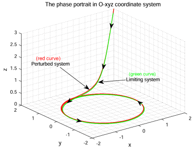
(a) The projection of the flow $\phi_{t}(x_{0},y_{0},z_{0},w_{0})$ in space O-xyz and the flow $\psi_{t}(x_{0},y_{0},z_{0})$ of limiting system (4.2).

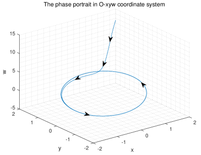
(b) The projection of the flow $\phi_{t}(x_{0},y_{0},z_{0},w_{0})$ in space O-xyw.

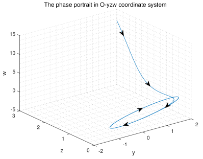
(c) The projection of the flow $\phi_{t}(x_{0},y_{0},z_{0},w_{0})$ in space O-yzw.

(d) The projection of the flow $\phi_{t}(x_{0},y_{0},z_{0},w_{0})$ in space O-xzw.

Fig 2: The corresponding phase portraits of Fig 1.

Remark 4.2.

Define the set $K=\{\xi\in\mathbb{R}^{3}:\langle P\xi,\xi\rangle\geq 0,\langle\xi,v_{+}\rangle\geq 0\}$, where $v_{+}$ is an eigenvector of $P$ with respect to the positive eigenvalue $1$. It is clear that $K$ is a usual convex cone with nonempty interior. Moreover, the set $C=\{\xi\in\mathbb{R}^{3}:\langle P\xi,\xi\rangle\leq 0\}$ can be written as $C=\overline{\mathbb{R}^{3}\backslash(K\cup(-K))}$. We say a flow $\psi_{t}$ is strongly competitive with respect to the partial ordering induced by $K$ if $y-x\in\text{Int }K$ whenever $\psi_{t}(y)-\psi_{t}(x)\in K\backslash\{0\}$ and $t>0$.

We emphasize that a flow $\psi_{t}$ is strongly monotone with respect to $C$ if and only if $\psi_{t}$ is strongly competitive; and moreover, $D\psi_{t}(x)[C\backslash\{0\}]\subset\text{Int }C$ for $x\in U$ and $t>0$ if and only if $D\psi_{-t}(\psi_{s}(x))[K\backslash\{0\}]\subset\text{Int }K$ for $x\in U$, $0<t\leq s$.

As a consequence, the fact that system (4.2) is $C$-cooperative implies that its flow $\psi_{t}^{0}$ satisfies that $D\psi_{-t}^{0}(\xi)[K\backslash\{0\}]\subset\text{Int }K$ for $t>0$ and $-t\in I(\xi)$, where $I(\xi)\subset\mathbb{R}$ denotes the maximal interval of existence of the solution passing though $\xi$. By our previous work in [18, 17], there exists a positive constant $\epsilon_{*}<\epsilon_{0}$ such that for each $\epsilon\in(0,\epsilon_{*})$, the $\omega$-limit set of (4.1) is equivalent to an $\omega$-limit set of an eventually competitive system. Moreover, if the orbit passing though any point $\zeta=(x,y,z,w)\in D_{\epsilon}$ is tracked by a full orbit in $K_{\epsilon}$, then the $\omega$-limit set $\omega(\zeta)$ containing no equilibrium is a single closed orbit. The main result in the present paper provides a different view that a flow which is competitive can be viewed as a monotone system with respect to a high-rank cone, by which we can ignore the priori drawback restriction of the so called Non-oscillation Principle for the full orbits in competitive systems.

References

• [1] N. Fenichel, Geometric singular perturbation theory for ordinary differential equations, J. Diff. Equ., 31(1979), 53-98.
• [2] G. Fusco and W. Oliva, A Perron theorem for the existence of invariant subspaces, Ann. Mat. Pura. Appl., 160(1991), 63-76.
• [3] L. Feng, Y. Wang and J. Wu, Semiflows “monotone with respect to highrank cones” on a Banach space, SIAM J. Math. Anal., 49(2017), 142-161.
• [4] L. Feng, Y. Wang and J. Wu, Generical behavior of flows strongly monotone with respect to high-rank cones, J. Differential Equations, 275 (2021), 858–881.
• [5] P. Hess and P. Poláčik, Boundeness of prime periods of stable cycles and convergence to fixed points in discrete monotone dynamical systems, SIAM J. Math. Anal. 24(1993), 1312-1330.
• [6] M. W. Hirsch, Systems of differential equations which are competitive or cooperative I: limit sets, SIAM J. Appl. Math., 13 (1982), 167–179.
• [7] M. W. Hirsch, Systems of differential equations which are competitive or cooperative II: convergence almost everywhere, SIAM J. Math. Anal., 16(1985), 423-439.
• [8] M. W. Hirsch, Systems of differential equations which are competitive or cooperative III: compting species, Nonlinearity, 1 (1988), 51–71.
• [9] M. W. Hirsch, Systems of differential equations which are competitive or cooperative IV: Structural stability in three dimensional systems, SIAM J. Math. Anal., 21 (1990), 1225–1234.
• [10] M. W. Hirsch, Systems of differential equations that are competitive or cooperative V: convergence in $3$-dimensional systems, J. Differential Equations, 80 (1989), 94–106.
• [11] M. W. Hirsch, Systems of differential equations that are competitive or cooperative VI: a local $C^{r}$ closing lemma for $3$-dimensional systems, Ergodic Theory Dynam. Systems, 11 (1991), 443–454.
• [12] M. W. Hirsch and H. L. Smith, Monotone Systems, A Mini-review, Proceedings of the First Multidisciplinary Symposium on Positive Systems (POSTA 2003), Luca Benvenuti, Alberto De Santis and Lorenzo Farina (Eds.) Lecture Notes on Control and Information Sciences Vol. 294, Springer-Verlag, Heidelberg, 2003.
• [13] M. W. Hirsch and H. L. Smith, Monotone dynamical systems, Handbook of Differential Equations: Ordinary Differential Equations, Vol. 2, Elsevier, Amsterdam 2005.
• [14] C.K.R.T. Jones, Geometric singular perturbation theory, Dynamical Systems (Montecatini Terme,1994). Lect. Notes in Math., 1609, Springer, Berlin, 1995.
• [15] M. A. Krasnosel’skii, J. A. Lifshits and A. V. Sobolev, Positive Linear Systems, the Method of Positive Operators, Heldermann Verlag, Berlin, 1989.
• [16] K. Nipp, Smooth attractive invariant manifolds of singularly perturbed ODE’s, Research Report, (1992), 92–13.
• [17] Lin Niu, Eventually competitive systems generated by perturbations, Electronic Journal of Differential Equations, 121(2019), 1-12.
• [18] Lin Niu and Yi Wang, Non-oscillation principle for eventually competitive and cooperative systems, Discrete Contin. Dyn. Syst. B, 24 (2019), 6481-6494.
• [19] R. Ortega and L. Sánchez, Abstract competitive systems and orbital stability in $\mathbb{R}^{3}$, Proc. Amer. Math. Soc., 128(2000), 2911-2919.
• [20] P. Poláčik, Convergence in smooth strongly monotone ows defined by semilinear parabolic equations, J. Differential Equations, 79(1989), 89-100.
• [21] P. Poláčik, Generic properties of strongly monotone semiflows defined by ordinary and parabolic differential equations, Qualitative theory of differential equations (Szeged 1988), 519-530, Colloq. Math. Soc. János Bolyai, 53, North-Holland, Amsterdam, 1990.
• [22] P. Poláčik and I. Tereščák, Convergence to cycles as a typical asymptotic behavior in smooth strongly monotone discrete-time dynamical systems, Arch. Ration. Mech. Anal. 116(1992), 339-360.
• [23] K. Sakamoto, Invariant manifolds in singular perturbation problems for ordinary differential equations, Proc. R. Soc. Edinb. A, 116(1990), 45-78.
• [24] L. A. Sánchez, Cones of rank $2$ and the Poincaré-Bendixson property for a new class of monotone systems, J. Differential Equations, 216(2009), 1170-1190.
• [25] H. L. Smith, Monotone Dynamical Systems, an introduction to the theory of competitive and cooperative systems, Math. Surveys and Monographs, 41, Amer. Math. Soc., Providence, Rhode Island 1995.
• [26] H. L. Smith, Monotone dynamical systems: Reflections on new advances and applications, Discrete Contin. Dyn. Syst., 37(2017), 485-504.
• [27] H. Smith and H. Thieme, Quasi convergence and stability for strongly order-preserving semiflows, SIAM J. Math. Anal. 21(1990), 673-692.
• [28] R. A. Smith, The Poincaré-Bendixson theorem for certain differential equations of higher order, Proc. of Royal Soc. of Edinburgh, 83A(1979), 63-79.
• [29] R. A. Smith, Existence of periodic orbits of autonomous ordinary differential equations, Proc. of Royal Soc. of Edinburgh A, 85(1980), 153-172.
• [30] R. A. Smith, Orbital stability for ordinary differential equations, J. Differential Equations, 69(1987), 265-287.
• [31] I. Tereščák, Dynamics of $C^{1}$ smooth strongly monotone discrete-time dynamical systems, preprint, Comenius University, Bratislava, 1994.
• [32] L. Wang and E. D. Sontag, Singularly perturbed monotone systems and an application to double phosphorylation cycles, J. Nonlinear Sci., 18(2008), 527-550.
• [33] Y. Wang and J. Yao, Dynamics alternatives and generic convergence for $C^{1}$-smooth strongly monotone discrete dynamical systems, J. Differential Equations, 269(2020), 9804-9818.
• [34] E. Weiss and M. Margaliot, A generalization of linear positive systems with applications to nonlinear systems: Invariant sets and the Poincaré-Bendixson property, Automatica J.IFAC, 123, 2021.