Contact-timing and Trajectory Optimization for 3D Jumping on Quadruped Robots

Abstract

Performing highly agile acrobatic motions with a long flight phase requires perfect timing, high accuracy, and coordination of the full-body motion. To address these challenges, we present a novel approach on timings and trajectory optimization framework for legged robots performing aggressive 3D jumping. In our method, we firstly utilize an effective optimization framework using simplified rigid body dynamics to solve for contact timings and a reference trajectory of the robot body. The solution of this module is then used to formulate a full-body trajectory optimization based on the full nonlinear dynamics of the robot. This combination allows us to effectively optimize for contact timings while ensuring that the jumping trajectory can be effectively realized in the robot hardware. We first validate the efficiency of the proposed framework on the A1 robot model for various 3D jumping tasks such as double-backflips off the high altitude of 2m. Experimental validation was then successfully conducted for various aggressive 3D jumping motions such as diagonal jumps, barrel roll, and double barrel roll from a box of heights 0.4m and 0.9m, respectively.

I Introduction

In the last decade, there has been a rapid development of legged robots, allowing them to effectively traverse rough terrain. Especially, the realization of jumping behaviors on legged robots has greatly drawn research attention because of their advantages in navigating high obstacles [1],[2],[3],[4].

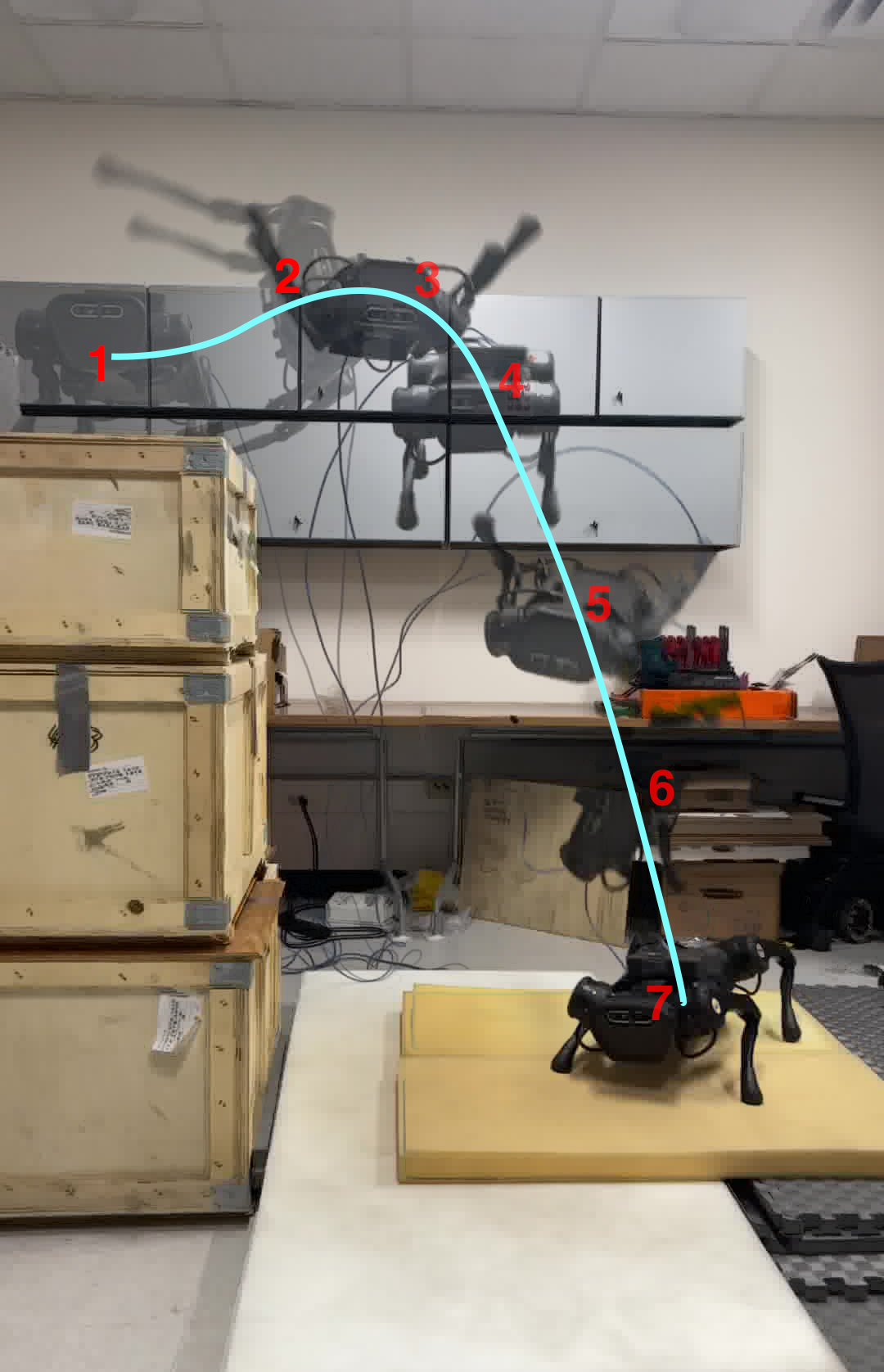
Figure 1: A combined motion snapshot of the Unitree A1 robot performing a double barrel roll from a $0.9m$ platform. Experiment and simulation video: %****␣Introduction.tex␣Line␣25␣****https://youtu.be/d7RcWEXTbqc.

There exists a number of dynamic models of legged robots, which are commonly utilized by optimization and control frameworks to realize agile locomotion. Single rigid body dynamics (SRBD) is widely used for control of legged robots. This simplified model considers the effect of ground reaction forces on the robot body while ignoring the leg dynamics, which enables real-time computation, e.g., Model Predictive Control (MPC), to achieve highly dynamic motions in [2],[5],[6],[7]. However, real-time MPC typically requires a limited prediction horizon when planning these motions. While the SRBD model is a suitable choice for online execution, the full-body dynamics can be adopted when the model accuracy is crucial [4],[8]. Acrobatic jumping motions usually require a long aerial phase and high accuracy of full-body coordination for all contact phases. Thus, it is essential to consider the full-body dynamics. In our prior work [4], we have introduced an effective trajectory optimization framework that allows MIT Cheetah 3 jumping on a high platform. However, this framework is primarily designed for 2D motion with a predefined contact schedule. In this paper, we present a unified framework to optimize for contact schedule and 3D jumps on legged robots.

Centroidal dynamics and full-body kinematics constraints are also used in trajectory optimization to execute agile motions [3],[9]. They reduces the complexity of dynamics compared to the full-body dynamics, while considering the feasibility of kinematic motions. Regarding the quadruped jumping, a recent work in [3] combines trajectory optimization using the centroidal dynamics and a whole-body controller to track the reference motions from the optimization. Difference from [3], we optimize contact timings and leverage the full nonlinear dynamics of the robot, which allows us to achieve highly accurate jumps such as multiple backflips and barrel rolls (see Fig. 1).

While there is an increasing number of work attempts to find optimal contact timings for agile motions [10],[11],[12],[13], the contact timings optimization for highly dynamic 3D jumps has not been well explored. The recent work [12] proposes a trajectory optimization (TO) approach based on SRBD to solve for contact timings. However, since this work uses a linearized rigid body dynamics using Euler angle representation, it offers a limited range of achievable motions due to the singularity [14]. In our work, we are interested in optimizing the contact timings for highly aggressive and complex 3D jumps with long aerial time. We utilize a rotation matrix to represent body orientation to prevent the singularity and unwinding issues associated with Euler angle and quaternion representation [14]. In addition, difference from [12] , the solution of our proposed contact-timing optimization is then utilized to formulate the full-body TO that considers torque constraints and the whole-body coordination. Therefore, our framework enables aggressive jumps to be realized in the robot hardware.

The contribution of the work is summarized as follows. Firstly, we propose a contact-timing optimization method to simultaneously solve for optimal contact timings and reference trajectory of the robot body, which will then be used to formulate a full-body trajectory optimization. Secondly, in the contact-timing optimization, the rotation matrix is directly utilized to represent the orientation of the robot body to avoid singularity and unwinding issues. This utilization allows us to optimize for a wide range of complex 3D jumping motions. We also present a full-body trajectory optimization to perform a diverse set of aggressive 3D jumping tasks that require high accuracy and long aerial time. Finally, our proposed framework is validated in both experiment and the A1 robot model for various gymnastic 3D jumping tasks, e.g., double-backflips and double barrel roll from boxes of height 2m and 0.9m.

The rest of our paper is organized as follows. The optimization framework are presented in Section II; jumping and landing controllers are briefly described in Section III. Results from selected hardware experiments are presented in Section IV. Finally, Section V provides concluding remarks.

II Contact-timing optimization

II-A Motivation

When performing highly dynamic and complex jumping in 3D, it is critical to leverage the full-body dynamics of the robot to maximize the jumping performance and guarantee the high accuracy of the jumping trajectory while realizing in the real robot hardware.

In the full-body trajectory optimization, contact timing is predefined for each jumping phase [4]. During the flight phase of the jumping motion, the robot motion has minimal effect in the COM trajectory of the robot. Therefore, it is critical to optimize for the contact schedule, especially with motions that have a significant aerial time. Moreover, the manual selection of the timings is time-consuming, not optimal, and even it is not feasible for the full-body trajectory optimization to obtain solutions for many complex 3D jumps. Therefore, it is crucially important to implement an approach to automatically compute optimal timings. Furthermore, timings in highly dynamic motion with long flight phase plays a crucial role in minimizing the effort or energy, guaranteeing the feasibility of the motion within the limits of actuator powers.

In the following, we introduce a framework that includes optimal contact timings and full-body trajectory optimization to generate complex 3D jumping motions at high accuracy.

II-B Contact timings optimization

A direct implementation of contact-timing optimization using the full nonlinear dynamics of the robot takes considerable time to solve due to the high complexity of the problem. In our implementation, it does not even produce a feasible solution for many complex 3D jumps. Therefore, these issues motivate us to take advantage of the simplified dynamics to optimize for contact timings. Section II-B presents our contact-timing optimization framework to obtain the optimal contact schedule and body reference trajectory, which then be used to formulate the full-body trajectory optimization introduced in Section II-C. The overview of our approach is illustrated in Fig. 2.

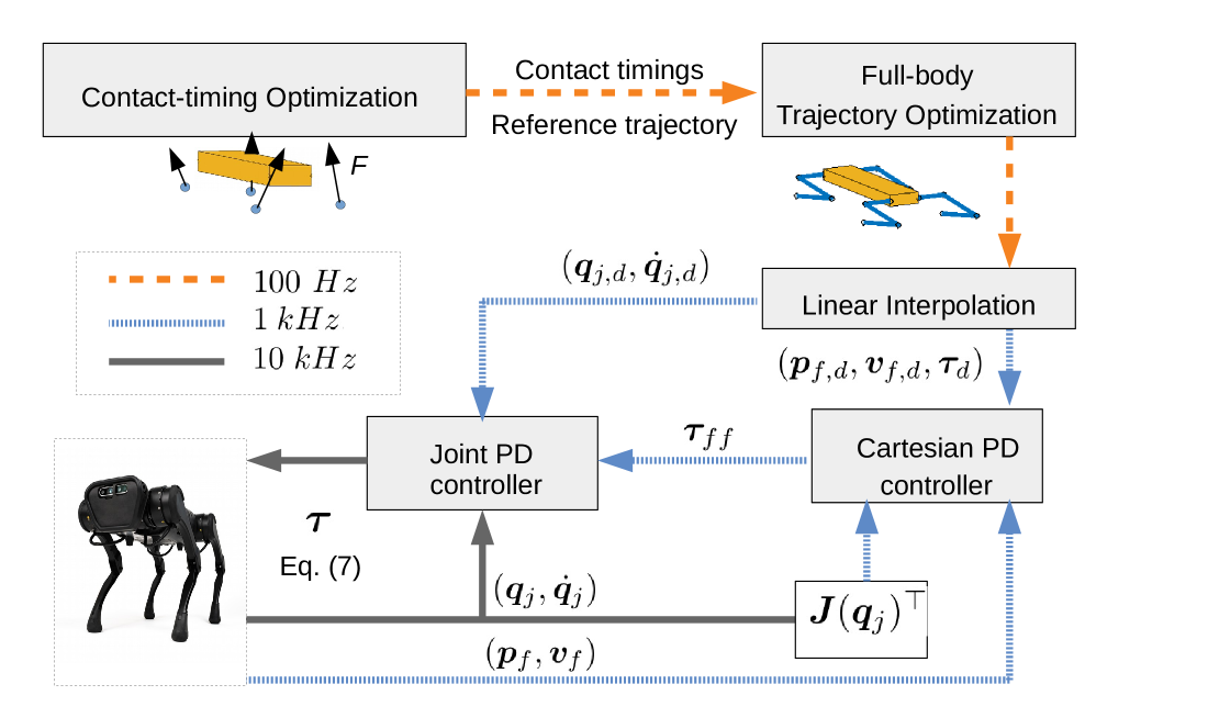
Figure 2: Block diagram of the propose framework.

TABLE I: Optimal contact timings $T_{i}$, solving time via IPOPT for the contact-timing optimization in Section II-B, and full-body trajectory optimization in Section II-C

Jumps	Optimal timings	Solving time	Solving time
	$T_{i}$ ($\times 10ms$)	contact-timing	full-body
		optimization	TO
lateral 30cm	50, 28	4.14 [s]	31 [s]
lateral down	52, 35	5.02 [s]	32 [s]
$90^{0}$ spinning	56, 31	5.7 [s]	39 [s]
diagonal jump	54, 30, 33	5.98 [s]	226 [s]
barrel roll	51, 32, 35	6.61 [s]	35 [s]
double barrel roll	52, 34, 55	11.7 [s]	46 [s]
double backflip	50, 33, 69	7.23 [s]	89 [s]

Unlike [3] and [12], which use Euler angles, we use a rotation matrix to represent the body orientation when planning 3D jumping motions. Given the sequence of contacts, we will optimize their duration (i.e., contact timings). We choose Cartesian space to derive the SRB’s equation of motion:

$$\ddot{\bm{p}} =\sum_{s=1}^{n_{s}}\bm{f}^{s}/m-\bm{g},$$ (1a)

$$\bm{I_{b}}\dot{\bm{\Omega}}+\bm{\Omega}\times\bm{I_{b}}\bm{\Omega} =\bm{R}^{-1}\sum_{s=1}^{n_{s}}\bm{f}^{s}\times(\bm{p}-\bm{p}_{f}^{s}),$$ (1b)

$$\dot{\bm{R}} =\bm{R}\widehat{\mathbf{\Omega}}$$ (1c)

where $n_{s}$ is number of feet, m is the robot’s mass, $\bm{\Omega}\in\mathbb{R}^{3}$ is angular velocity expressed in the body frame, $\bm{R}$ is rotation matrix of the body frame, $\bm{g}$ is the gravity acceleration; $\bm{p},\dot{\bm{p}},\ddot{\bm{p}}\in\mathbb{R}^{3}$ is the CoM position, velocity, acceleration of the body in the world frame; $\bm{f}^{s}\in\mathbb{R}^{3}$ is GRF on foot $s^{th}$; $\bm{p}_{f}^{s}\in\mathbb{R}^{3}$ is $s^{th}$ foot position in the world frame. The hat map $(\hat{.}):\mathbb{R}^{3}\rightarrow so(3)$ converts any vector in $\mathbb{R}^{3}$ to the space of skew-symmetric matrices. For the sake of notation, we define the robot’s state as $\bm{x}:=\left[\bm{p};\dot{\bm{p}};\bm{\Omega};\dot{\bm{\Omega}};\bm{R}\right]$. The contact-timing optimization is then formulated as follows:

$$\underset{\bm{x},\bm{f},\bm{e}_{R}}{\text{minimize}}\textrm{ }\sum_{k=1}^{N^{c}}\epsilon_{\Omega}\bm{\Omega}_{k}^{T}\bm{\Omega}_{k}+\epsilon_{f}\bm{f}_{k}^{T}\bm{f}_{k}+{\color[rgb]{0,0,0}\epsilon_{R}\bm{e}_{R_{k}}^{T}\bm{e}_{R_{k}}}$$

s.t. $$[\bm{R},\bm{p},\bm{p}_{f}^{s}](k=1)=[\bm{R}_{0},\bm{p}_{0},\bm{p}_{f,0}^{s}],~{}\textrm{{initial states}}$$ (2a)

$$[\bm{\Omega},\dot{\bm{\Omega}},\dot{\bm{p}}](k=1)=\bm{0},~{}~{}~{}~{}~{}~{}~{}~{}~{}~{}~{}~{}~{}~{}~{}~{}\textrm{{initial states}}$$ (2b)

$$[\bm{R},\bm{p},\bm{p}_{f}^{s}](k=N^{c})=[\bm{R}_{g},\bm{p}_{g},\bm{p}_{f,g}^{s}],\textrm{{final states}}$$ (2c)

$$|\bm{R}(k)[\bm{p}_{f}^{s}(k)-\bm{p}(k)]-\bar{\bm{p}}_{f}^{s}(k)|\leq\textbf{r},\textrm{{foot position}}$$ (2d)

$${\color[rgb]{0,0,0}|\bm{f}_{k}^{s,x}/\bm{f}_{k}^{s,z}|\leq\mu,|\bm{f}_{k}^{s,y}/\bm{f}_{k}^{s,z}|\leq\mu,~{}~{}\textrm{{friction cone}}}$$ (2e)

$${\color[rgb]{0,0,0}\bm{f}_{k,min}^{s}\leq\bm{f}_{k}^{s,z}\leq\bm{f}_{k,max}^{s},~{}~{}~{}~{}~{}~{}~{}~{}~{}~{}~{}~{}~{}\textrm{{GRF limits}}}$$ (2f)

$${\color[rgb]{0,0,0}\bm{p}_{k,min}\leq\bm{p}_{k}\leq\bm{p}_{k,max},~{}\textrm{{CoM in contact phases}}}$$ (2g)

$$\gamma(\bm{x}_{k},\bm{x}_{k+1},\bm{f}(k),\bm{p}_{f}^{s}(k))=0,~{}\textrm{{discrete dynamic}}$$ (2h)

$${\color[rgb]{0,0,0}\bm{R}_{k+1}=\bm{R}_{k}exp(\widehat{\bm{\Omega}_{k}T_{i}/N_{i}})},~{}~{}~{}~{}~{}\textit{SO(3) manifold}$$ (2i)

$$\sum_{i=1}^{n_{p}}T_{i}\in[T_{min},T_{max}],~{}N^{c}=\sum_{i=1}^{n_{p}}N_{i}$$ (2j)

$$\textrm{ for }\textrm{ }k=1,2,...N^{c}$$

where $\bm{\Omega}_{k}\in\mathbb{R}^{3}$, $\bm{f}_{k}\in\mathbb{R}^{12}$ is angular velocity of SRB w.r.t the body frame, and GRF on four legs at the iteration $k^{th}$; $\epsilon_{\Omega},\epsilon_{f},\epsilon_{R}$ are cost function weights of corresponding elements, and $\epsilon_{R},\epsilon_{\Omega}>>\epsilon_{f}$. We use an error term of rotation matrix as $\bm{e}_{R_{k}}=log(\bm{R}_{ref,k}^{T}.\bm{R}_{k})^{\vee}$, where $log(.):SO(3)\rightarrow so(3)$ is the logarithm map, and the vee map $(.)^{\vee}:so(3)\rightarrow\mathbb{R}^{3}$ is the inverse of hat map [14],[15]. With given final and initial rotation matrix, $\bm{R}_{g}$ and $\bm{R}_{0}$ respectively, we utilize a linear interpolation to obtain $\bm{R}_{ref,k}$ at $k^{th}$ step. The equation (2d) implies that the $s^{th}$ foot position is constrained inside a sphere $\mathcal{S}_{s}$ of radius r so that the joint angle are within limits. The center of the sphere $\bar{\bm{p}}_{f}^{s}(k)$ is relative to the CoM position. The function $\gamma(.)$ captures the dynamic constraints discretized from (1a)-(1b) via the forward Euler method.

In (2j), $n_{p}$ is a number of contact phases. For example, if the pre-selected contact schedule is four-leg contact, rear-leg contact, and flight phase, then $n_{p}=3$. $N_{i}$ is the predefined number of time steps for the $i^{th}$ contact phase, $i\in\left\{1,2,..,n_{p}\right\}$. Note that our approach solves for optimal timing $T_{i}$, given a total predefined interval $[T_{min},T_{max}]$. The equation (2i) is derived from (1c) to ensure $\bm{R}_{k}$ evolves in the SO(3) manifold. Here, $exp(.):so(3)\xrightarrow[]{}SO(3)$ is known as the matrix exponential map.

Remark 1

Despite the advantage of using a rotation matrix $\bm{R}$ to achieve the most 3D jumping motions, utilizing it in the trajectory optimization setup introduces more optimization variables and constraints. This significantly increases the problem size and solving time. To achieve a feasible solution, $\bm{R}$ in (2i) must be approximated at high accuracy enough to satisfy the $SO(3)$ property at every time step. Taylor series approximation at a high degree is utilized for that purpose. However, choosing a really high degree of Taylor’s approximation is prohibitively costly in terms of computational time. Therefore, in order to balance accuracy and solving time, we utilize the $4^{th}$ degree of Taylor’s series: $exp(\mathbf{A})=\sum_{k=0}^{4}\frac{\mathbf{A}^{k}}{k!}.$ Moreover, for complex jumping motions in 3D, adding and minimizing the term $\bm{e}_{R_{k}}^{T}\bm{e}_{R_{k}}$ in the cost function in (2) helps to guide the trajectory optimization toward a feasible solution in a fast manner.

II-C Full-body trajectory optimization for 3D jumping

When performing highly dynamic jumping, it is important to consider the full nonlinear dynamics of the robot in the optimization framework. This will guarantee the accuracy of the jumping trajectory while transferring to the hardware.

II-C1 Full-body dynamics model

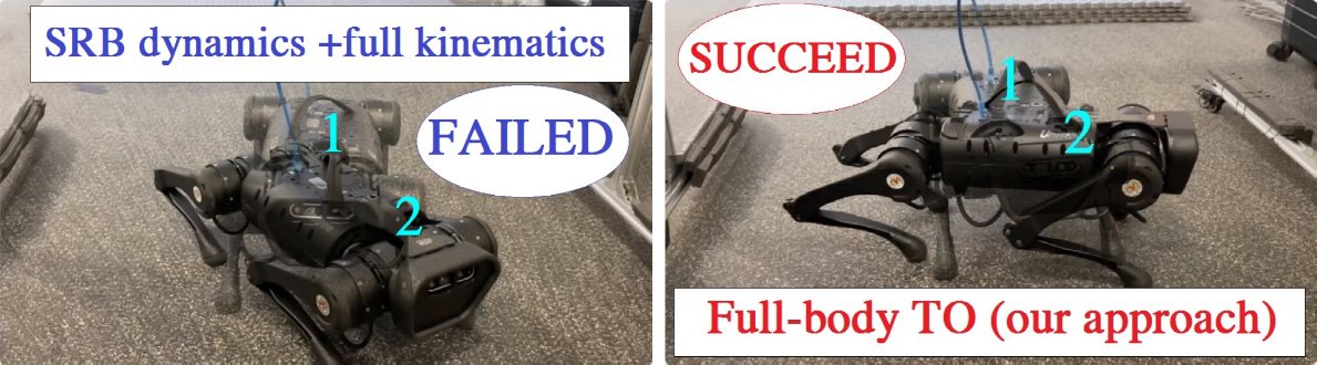
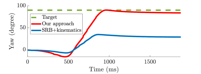
Figure 3: Comparison between trajectory optimization of SRB dynamics+ full-body kinematics constraints approach and full-body TO (our approach) for a $90^{0}$ spinning jump target in experiment.

The robot is modeled as a rigid-body system, and spatial vector algebra in [16] is used to construct the robot’s equations of motion:

$$\begin{bmatrix}\bm{H}&-\bm{J}_{s}^{T}\\ -\bm{J}_{s}^{T}&\mathbf{0}\end{bmatrix}\begin{bmatrix}\bm{\ddot{q}}\\ \bm{F}_{s}\end{bmatrix}=\begin{bmatrix}-\bm{C}\bm{\dot{q}}-\bm{g}+\bm{B}\bm{\tau}+\bm{B}_{f}\bm{\tau}_{f}\\ \bm{\dot{J}}_{s}(\bm{q})\bm{\dot{q}}\end{bmatrix}$$ (3)

where $\bm{q}:=\left[\bm{q}_{b};~{}\bm{q}_{j}\right]$ is a vector of generalized coordinates, in which $\bm{q}_{b}$ represents CoM position and orientation of the robot body, and $\bm{q}_{j}\in\mathbb{R}^{12}$ is a vector of joint angles. The mass matrix is denoted by $\bm{H}$; the matrix $\bm{C}$ is represented for Coriolis and centrifugal terms; $\bm{g}$ is the gravity vector; $\bm{J}_{s}$ is the spatial Jacobian of the body containing the $s^{th}$ contact foot, expressed at the foot and in the world coordinate system; $\bm{B}$ and $\bm{B}_{fric}$ are distribution matrices of actuator torques $\bm{\tau}$ and the joint friction torques $\bm{\tau}_{fric}$; $\bm{F}_{s}$ is the spatial force at the $s^{th}$ contact foot.

II-C2 Cost function and constraints

The ultimate goal of our framework is to find a feasible jumping motion for each 3D jumping task with the full rigid-body dynamics consideration. Due to the high complexity of this problem, the feasibility domain is limited. Therefore, the purpose of this cost function is to guide the optimization to converge to a feasible solution where the robot’s coordinates stays close to the reference configuration $\bm{q}_{ref}$ if possible. The CoM position and body orientation obtained from Section II-B are also linearly interpolated to get their profiles sampling at $dt=10~{}ms$, which is then used as reference for the full-body TO here. The cost function is defined as follows:

$$J= \sum_{h=1}^{N-1}\epsilon_{q}(\bm{q}_{h}-\bm{q}_{ref,h})^{T}(\bm{q}_{h}-\bm{q}_{ref,h})+\epsilon_{\tau}\bm{\tau}_{h}^{T}\bm{\tau}_{h}$$

$$+\epsilon_{N}(\bm{q}_{N}-\bm{q}_{N}^{d})^{T}(\bm{q}_{N}-\bm{q}_{N}^{d}),$$ (4)

where $N$ denotes the total of the time steps (i.e. $N=T_{opt}/dt$ with $T_{opt}$ is optimal total time obtained from Section II-B; $\bm{q}_{h},\bm{\tau}_{h}$ are the generalized coordinates and joint torque at the iteration $h^{th}$; $\bm{q}_{N}$ is the the generalized coordinates at the end of the trajectory; the first six elements of $\bm{q}_{ref,h}$ is the reference CoM position and body orientation obtained from contact timing optimization in Section II-B. The last 12 elements of $\bm{q}_{ref,h}$ is set to be the final joint configuration. We also use $\bm{q}_{ref,h}$ as initial guess for the TO to reduce the solving time. $\epsilon_{q},\epsilon_{\tau},\epsilon_{N}$ are cost function weights of corresponding elements. The following constraints are:

• Full-body dynamics constraints (3)

• Initial configuration: $\bm{q}(h=0)=\bm{q}_{0},\bm{\dot{q}}(h=0)=\bm{0}$.

• Pre-landing configuration: $\bm{q}_{j,h}=\bm{q}_{h,N}^{d},\bm{\dot{q}}_{j,h}=\bm{0}~{}(h\in[(N-a):N])$, where $a$ is a jumping task-based selection ($a<N$).

• Final configuration: $\bm{q}_{h}(h=N)=\bm{q}_{N}^{d}$.

• Joint angle constraints: $\bm{q}_{j,min}\leq\bm{q}_{j,h}\leq\bm{q}_{j,max}$

• Joint velocity constraints: $|\bm{\dot{q}}_{j,h}|\leq\bm{\dot{q}}_{j,max}$

• Joint torque constraints: $|\bm{\tau}_{h}|\leq\bm{\tau}_{max}$

• Friction cone limits: $|\bm{F}_{h}^{x}/\bm{F}_{h}^{z}|\leq\mu$, $|\bm{F}_{h}^{y}/\bm{F}_{h}^{z}|\leq\mu$

• Minimum GRF: $\bm{F}_{h}^{z}\geq\bm{F}_{min}^{z}$

• Geometric constraints to guarantee: (i) each robot part does not collide with others, (ii) the whole robot body and legs have a good clearance with obstacle.

III Jumping and Landing Controller

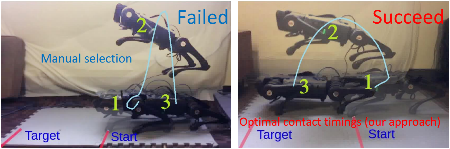
Figure 4: Experiments: Motion snapshots from jumping forward with manual selection of contact timings in the left figure and optimal contact timings (our approach) in the right figure.

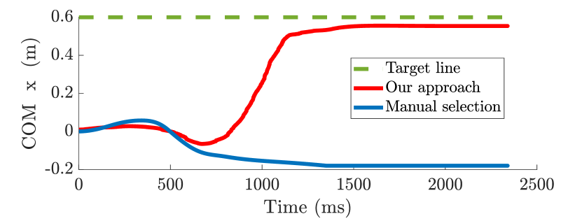
(a) Trajectory comparison

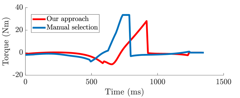
(b) Thigh torque of rear legs

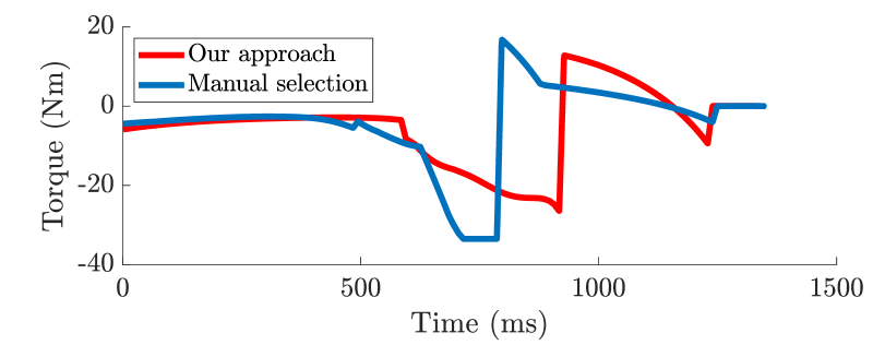
(c) Calf torque of rear legs

Figure 5: Comparison between manual selection and optimal contact timings (our approach) The comparison is considered based on target achievement from experiments in Fig. 5a, and the feed forward torque of rear legs generated from the full-body TO for jumping forward $0.6~{}m$ under manual selection of contact timings and optimal contact timing (our approach) in Fig. 5b & 5c. The Fig. 5 is accompanied with the Fig. 4.

Having introduced the full-body optimization approach, in this section we present a jumping and landing controller to help robot tracking the reference trajectory and effectively handle the high impact with the ground when performing 3D aggressive jumps off from high altitude (see Fig.2). The desired joint angle $\bm{q}_{d}$, joint velocity $\bm{\dot{q}}_{d}$, foot position $\bm{p}_{f,d}$ and foot velocity $\bm{v}_{f,d}$ w.r.t their hips, and feed-forward joint torque $\bm{\tau}_{d}$ are obtained from the full-body TO. They are then linearly interpolated to get new reference profiles at $1~{}kHz$. To track the reference trajectories, we use the feedback Cartesian PD controller that executes at $1~{}kHz$:

$$\bm{\tau}_{ff}=\bm{J}(\bm{q}_{j})^{\top}[\bm{K}_{p}(\bm{p}_{f,d}-\bm{p}_{d})+\bm{K}_{d}(\bm{v}_{f,d}-\bm{v}_{f})]+\bm{\tau}_{d}$$

where $\bm{J}(\bm{q}_{j})$ is the foot Jacobian at $\bm{q}_{j}$; $\bm{K}_{p}$ and $\bm{K}_{d}$ are diagonal matrices of proportional and derivative gains. The joint PD controller running at $10~{}kHz$ in the low-level motor control is integrated to improve the tracking performance. The full controller for tracking desired trajectories is:

$$\bm{\tau}=\bm{\tau}_{ff}+\bm{K}_{p,joint}(\bm{q}_{j,d}-\bm{q})+\bm{K}_{d,joint}(\bm{\dot{q}}_{j,d}-\bm{\dot{q}}).$$ (5)

Since there always exists a model mismatch between the optimization and hardware, it normally has orientation angle errors upon landing. Therefore, we utilize a real-time landing controller to handle impact, control GRF, balance the whole body motion during the landing phase, and recover the robot from unexpected landing configurations. For that controller, we extend the proposed QP controller [4] for the 3D jumps:

$$\textbf{if}~{}~{}(\text{any}~{}c_{s}>=\delta)\&(t\geq T_{posing})$$

$$\textbf{then}~{}~{}~{}\text{switch to landing controller},$$

where $c_{s}$ is the value obtained from the contact sensor of the foot $s^{th}$, and $\delta$ is the force threshold to determine if the ground impact happened. $T_{posing}$ is the instant at the beginning of the pre-landing configuration (after that instant $\dot{\bm{q}}_{j}^{d}=0$). When the impact is detected in any foot, we switch from jumping to landing controller, then based on which foots are in contact, different robot models are used for the landing controller. Our experimental results validate that it is effective to use the QP landing controller for SRB to handle impact with the ground and balance the robot when landing.

Remark 2

Normally, all legs do not touch ground simultaneously due to the mismatch between the optimization model and hardware. Hence, utilizing a controller for swing legs also plays a crucial role here. Based on the contact model derived from the contact detection, the swing legs during landing phase are set at zero normal force and kept at the pre-landing configuration using PD controller until the ground contact is detected on these legs to prevent excessive impact force and unnecessarily extended movement.

Remark 3

For highly aggressive jumping motions, e.g. double barrel roll and double backflips, due to the high linear and angular velocity of robot body upon the ground impact, the robot continues to move and rotate in the current direction, which may cause unfavorable landing posture as observed in our experiments. To tackle this issue, we utilize a PD controller during the pre-landing configuration to extend the legs in that direction based on the body velocity reference obtained from trajectory optimization at the impact.

IV Results

This section presents experimental testing and simulation results with the commercial Unitree A1 robot [17]. A video of the results is included as supplementary material.

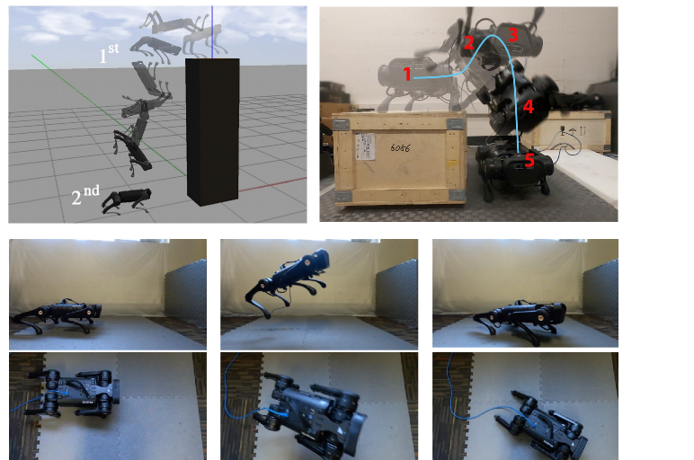
Figure 6: Other example of successful 3D jumping motions achieved via our proposed framework. The top left figure is a 3D double backflip from a box of height $2m$. The top right is a 3D barrel roll from a box of height $0.4m$. The figures in the last two rows are motion snapshots from a successful 3D diagonal jump $[x,y,yaw]=[0.4~{}m,-0.3~{}m,45^{0}]$ from a side and a top view in experiments.

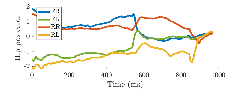
(a)

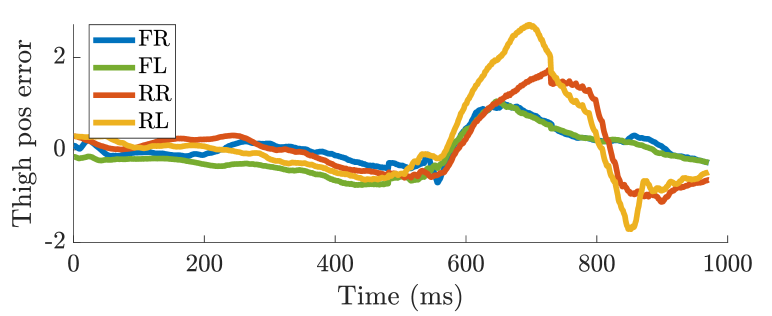
(b)

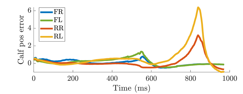
(c)

Figure 7: 3D diagonal jump in experiments. The figures are the tracking error of joint positions (degree) with jumping controller. FR, FL, RR and RL are used to denote front right, front leg, rear right, and rear left leg respectively.

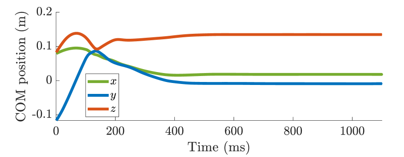
(a)

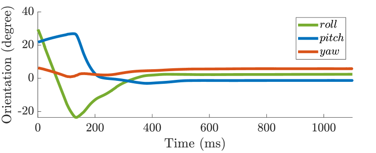
(b)

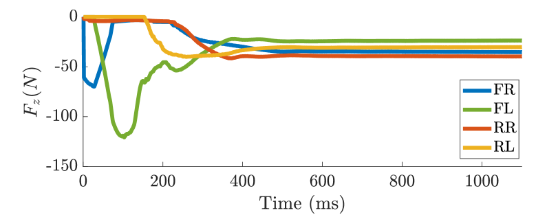
(c)

Figure 8: Landing controller for a double barrel roll jump in experiments. The plots show the COM position, body orientation, and force command during the landing phase when the robot performs a double barrel roll from a box with the height of $0.9~{}m$ (see Fig. 1).

IV-A Numerical Simulation

We use MATLAB and CasADi (see [18]) to construct and solve all presented trajectory optimization approaches for all 3D jumps. A user can predefine a contact sequence for the motion. For example, for the lateral and spinning jumps, we use a sequence of a four-leg contact and then a flight phase. For the total duration of the motion, we set $[T_{min},T_{max}]=[0.5,1.5](s)$ (see (2j)). With other jumping motions, the contact schedule is defined by a four-leg contact, a two-leg contact, and a flight phase, in which $[T_{min},T_{max}]=[1,2](s)$. For all jumps, we use $N_{i}=30$ for each contact phase. As shown in Table LABEL:tab:TO_solving_time, our approach computes optimal contact timings given a wide range of $[T_{min},T_{max}]$. It executes fast for all 3D jumps even with the high complexity of contact-timing optimization, which utilizes the rotation matrix representation. In addition, the full-body trajectory optimization is solved at a tractable time (less than 4 minutes) for all jumping motions given the high complexity of the full-body dynamics.

IV-B Experimental Validation

Firstly, in order to emphasize the importance of using full nonlinear dynamics model, we implement the trajectory optimization of SRBD + full-body kinematic constraints to compare with our proposed full-body trajectory optimization. In the first TO approach, constraints on joint torque $\bm{\tau}$ are imposed via joint angle $\bm{q}_{j}$ and ground reaction force $\bm{F}$ as the following simplification [3]: $\bm{\tau}_{min}\leq\bm{\tau}=J(\bm{q}_{j})^{T}\bm{F}\leq\bm{\tau}_{max}$, where $J(\bm{q}_{j})$ is the Jacobian of a leg. It is noted that in the first approach, the joint torque is not an optimization variable (similar to [3]). For the comparison, we pick a $90^{0}$ spinning jump with the contact schedule of (56,31) computed in Table LABEL:tab:TO_solving_time, to discuss here. As shown in Fig. 3, while our approach using the full-body dynamics guarantees a highly accurate jump, the trajectory optimization of SRBD and kinematic constraints fails to achieve the target angle. It has shown that the legs’ dynamics, which is neglected in the simplified dynamics, has a significant contribution in highly dynamic motions. Note that the comparison is made by directly applying joint PD controllers (5) to track the desired joint profiles obtained from these trajectory optimization approaches.

Secondly, we compare optimal contact timings with manually selected contact timings to show the advantage of the contact-timing optimization. Experiments for jumping forward $0.6~{}m$ are picked to discuss here (see Fig. 4 and Fig. 5). If timings are manually selected with unnecessary long flight time (e.g., $550~{}ms$), this makes the motor’s torque saturated in $100~{}ms$ that is up to $1/3$ of rear-leg contact phase. This selection seriously affects the motor working condition, causing failed joint tracking performance. Thus, the robot is unable to reach the target. On the other hand, selecting too small flight time makes the optimization unsolvable since the robot does not have enough power to jump to the desired configuration. By using optimal contact timings, we minimize the effort or energy, prevent the torque saturation issue, and execute successful jumps on the hardware.

Finally, we present the results of different aggressive 3D jumping experiments achieved by our framework that combines optimal contact timings and full-body TO. To the best of our knowledge, the results herein is the first implementation of full-body TO of quadruped robots for 3D jumping motions. We pick some jumping tasks to discuss here. In a successful diagonal jump (see Fig. 6), the jumping controller guarantees the high tracking performance as evident in Fig. 7. Using our approach, the robot can successfully performs a barrel roll from a box of height $0.4~{}m$ in experiments (see Fig. 6). Especially, with our proposed framework, the robot is able to complete a highly aggressive gymnastics double barrel roll jump, which is the first jump ever achieved by the quadrupedal robots (see Fig.1). These results illustrates the efficiency of our approach in optimizing the contact timings for the jumping task as well as the accuracy of the optimization framework when realizing in the robot hardware. In addition, these results also validate the effectiveness of the landing controller in handling hard impact. For that double barrel roll experiment, since the robot rotates with a high angular velocity from a high altitude, it has a considerably hard impact with the ground. However, the landing controller can recover the robot’s body position and orientation under the hard impact and significant error of landing configuration (see Fig. 8).

V Conclusions

This paper has introduced the framework for performing highly dynamics 3D jumps with long aerial time on quadruped robots that require model accuracy, perfect timings and coordination of the whole body motion. This framework combines contact timings of SRB dynamics, full-body TO, the jumping controller, and robust landing controller. The efficiency of the framework is validated via both A1 robot model and experiments on performing these aggressive tasks. The vision to autonomously detect obstacles will be integrated with the proposed framework in our future work.

References

- [1] Y. Ding and H.-W. Park, “Design and experimental implementation of a quasi-direct-drive leg for optimized jumping,” in 2017 IEEE/RSJ International Conference on Intelligent Robots and Systems (IROS), Vancouver, BC, Canada, IEEE, 2017.
- [2] H.-W. Park, P. M. Wensing, and S. Kim, “Jumping over obstacles with mit cheetah 2,” Robotics and Autonomous Systems, vol. 136, p. 103703, 2021.
- [3] M. Chignoli, “Trajectory optimization for dynamic aerial motions of legged robots,” MIT Libraries, 2021.
- [4] Q. Nguyen, M. J. Powell, B. Katz, J. D. Carlo, and S. Kim, “Optimized jumping on the mit cheetah 3 robot,” in 2019 International Conference on Robotics and Automation (ICRA), Canada, pp. 7448–7454, IEEE, 2019.
- [5] J. D. Carlo, P. M. Wensing, B. Katz, G. Bledt, and S. Kim, “Dynamic locomotion in the mit cheetah 3 through convex model-predictive control,” in 2018 IEEE/RSJ international conference on intelligent robots and systems (IROS), pp. 1–9, Oct 2018.
- [6] Y. Ding, A. Pandala, C. Li, Y. H. Shin, and H. W. Park, “Representation-free model predictive control for dynamic motions in quadrupeds,” IEEE Transactions on Robotics, pp. 1–18, 2021.
- [7] G. García, R. Griffin, and J. Pratt, “Time-varying model predictive control for highly dynamic motions of quadrupedal robots,” in 2021 International Conference on Robotics and Automation (ICRA), China, pp. 7344–7349, IEEE, 2021.
- [8] M. Posa, C. Cantu, , and R. Tedrake, “A direct method for trajectory optimization of rigid bodies through contact,” The International Journal of Robotics Research, vol. 33, pp. 69–81, 2014.
- [9] H. Dai, A. Valenzuela, and R. Tedrake, “Whole-body motion planning with centroidal dynamics and full kinematics,” in IEEE-RAS International Conference on Humanoid Robots, (Madrid, Spain), pp. 295–302, IEEE, 2014.
- [10] I. Mordatch, E. Todorov, and Z. Popovi, “Discovery of complex behaviors through contact-invariant optimization,” ACM Transactions on Graphics, vol. 31, pp. 1–8, 2012.
- [11] M. Neunert, F. Farshidian, A. W. Winkler, and J. Buchli, “Trajectory optimization through contacts and automatic gait discovery for quadrupeds,” IEEE Robotics and Automation Letters (RA-L), vol. 2, p. 1502–1509, 2017.
- [12] A. W. Winkler, C. D. Bellicoso, M. Hutter, and J. Buchli, “Gait and trajectory optimization for legged systems through phase-based end-effector parameterization,” IEEE Robotics and Automation Letters, vol. 3, pp. 1560–1567, 2018.
- [13] B. Ponton, A. Herzog, S. Schaal, and L. Righetti, “A convex model of momentum dynamics for multi-contact motion generation,” in IEEE-RAS International Conference on Humanoid Robots, p. 842–849, IEEE, 2016.
- [14] T. Lee, M. Leok, and N. H. McClamroch, “Geometric tracking control of a quadrotor uav on se(3),” in 49th IEEE Conference on Decision and Control, Atlanta, GA, USA, pp. 5420–5425, Dec 2010.
- [15] F. Bullo and A. D. Lewis, “Geometric control of mechanical systems: modeling, analysis, and design for simple mechanical control systems,” Springer Science & Business Media, vol. 49, no. 1, 2004.
- [16] R. Featherstone, Rigid body dynamics algorithms. Springer, 2014.
- [17] “Unitree a1 robot,” https://www.unitree.com/products/a1/.
- [18] J. A. E. Andersson, J. Gillis, G. Horn, J. B. Rawlings, and M. Diehl, “CasADi – A software framework for nonlinear optimization and optimal control,” Mathematical Programming Computation, In Press, 2018.