Efficient Estimation of Average Derivatives in NPIV Models:
Simulation Comparisons of Neural Network Estimators

Artificial Neural Networks (ANNs) can be viewed as nonlinear sieves that can approximate complex functions of high dimensional variables more effectively than linear sieves. We investigate the performance of various ANNs in nonparametric instrumental variables (NPIV) models of moderately high dimensional covariates that are relevant to empirical economics. We present two efficient procedures for estimation and inference on a weighted average derivative (WAD): an orthogonalized plug-in with optimally-weighted sieve minimum distance (OP-OSMD) procedure and a sieve efficient score (ES) procedure. Both estimators for WAD use ANN sieves to approximate the unknown NPIV function and are root-$n$ asymptotically normal and first-order equivalent. We provide a detailed practitioner’s recipe for implementing both efficient procedures. We compare their finite-sample performances in various simulation designs that involve smooth NPIV function of up to 13 continuous covariates, different nonlinearities and covariate correlations. Some Monte Carlo findings include: 1) tuning and optimization are more delicate in ANN estimation; 2) given proper tuning, both ANN estimators with various architectures can perform well; 3) easier to tune ANN OP-OSMD estimators than ANN ES estimators; 4) stable inferences are more difficult to achieve with ANN (than spline) estimators; 5) there are gaps between current implementations and approximation theories. Finally, we apply ANN NPIV to estimate average partial derivatives in two empirical demand examples with multivariate covariates.

JEL Classification: C14; C22

Keywords: Artificial neural networks; Relu; Sigmoid; Nonparametric instrumental variables; Weighted average derivatives; Optimal sieve minimum distance; Efficient influence; Semiparametric efficiency; Endogenous demand.

1 Introduction

Deep layer Artificial Neural Networks (ANNs) are increasingly popular in machine learning (ML), statistics, business, finance, and other fields. The universal approximation property of a variety of ANN architectures has been established by Hornik, Stinchcombe and White (1989) and many others. Early on, computational difficulties have hindered the wide applicability of ANNs. Recently, improvements in computing have led to successful applications of deep layer ANNs in computer vision, natural language processing and other areas, with complex nonlinear relations among many covariates and large data sets of high quality. Many problems where deep layer ANNs are extremely effective involve prediction problems (i.e. estimating conditional means or densities)—or problems in which nuisance parameters are themselves predictions. Recently, Farrell et al. (2018) and Athey, Imbens, Metzger and Munro (2019), among others, have applied multi-layer ReLU ANNs to estimate average treatment effects under unconfoundedness and demonstrated their good performance in estimating unknown conditional means and densities of multivariate covariates.It remains to be seen whether ANNs are similarly effective for structural estimation problems with nonparametric endogeneity.

To that end, we consider semiparametric efficient estimation and inference for a weighted average (partial) derivative (WAD) of a nonparametric instrumental variables regression (NPIV) via ANN sieves. Specifically, we assume an unknown structure function $h$ satisfies the NPIV model: $\mathbb{E}[Y_{1}-h(Y_{2})\mid X]=0$, where $Y_{2}$ is a continuous random vector of moderately high dimension (including endogenous regressors that are excluded from $X$), and $X$ is a vector of moderately high dimensional conditioning variables. We are interested in efficient estimation and inference for a WAD parameter of the smooth NPIV function $h(Y_{2})$, without sparsity assumptions on $h(\cdot)$.WADs of structural relationships are linked to elasticities of endogenous demand systems in economics. It is essentially a treatment effect parameter under confounding and endogenous continuous treatment. Although there is a large literature on efficient estimation of the average treatment effect and other causal parameters under unconfoundedness, there are far fewer results on efficient estimation and inference on the average treatment effect in nonparametric models with endogenous continuous treatment.

This paper makes three contributions. First, we present two classes of efficient estimators for WADs of NPIV models where unknown $h_{0}(Y_{2})$ is approximated by ANN sieves: the optimally weighted sieve minimum distance estimators and the efficient score-based estimators.Under some regularity conditions both types of estimators are root-$n$ asymptotically normal, semiparametrically efficient, and hence are first-order equivalent. Second, we detail a practitioner’s recipe that include a step by step guide for implementing these two classes of estimators. Third, and perhaps most importantly, we present a large set of Monte Carlo results on finite-sample performances of various ANN estimators. These are implemented using increasingly complex designs, such as NPIV function containing up to 13 continuous covariates (including endogenous regressors), various nonlinearities and correlations among the covariates.

We now briefly introduce the two classes of efficient estimation procedures that we consider. Both procedures are inspired by the semiparametric efficiency bound characterization in Ai and Chen (2012) (henceforth AC12) for the WAD of the unknown $h(Y_{2})$ in a NPIV model $\mathbb{E}[Y_{1}-h(Y_{2})\mid X]=0$. The first procedure is based on minimizing an optimal criterion, the optimally-weighted orthogonalized sieve minimum distance (SMD) criterion. This procedure is numerically equivalent to a semiparametric two-step procedure, where the unknown NPIV function $h(\cdot)$ is estimated via an optimally weighted SMD in the first step, and the WAD of $h(\cdot)$ is estimated using a sample analogue of an orthogonalized unconditional moment (Chamberlain, 1992) in the second step, with the unknown $h$ substituted by the optimally weighted SMD estimator from the first step. This will be denoted as OP-OSMD in our paper. AC12 already introduced this procedure and presented a small Monte Carlo study demonstrating its finite-sample performance using a spline SMD in the first step when the unknown $h(\cdot)$ is a function of a scalar endogenous variable $Y_{2}$. It is unclear how this procedure will perform when $Y_{2}$ could be a continuous random vector of higher dimension and when $h(\cdot)$ is approximated via a neural network.

The second procedure is based on the efficient score (equivalently, efficient influence function). AC12 derived a characterization of the efficient influence (or equivalently, efficient score) for the WAD of a NPIV model. It is also the asymptotic influence function of the OP-OSMD estimator. The efficient influence is the sum of the orthogonalized unconditional moment (the one used for the OP-OSMD estimator) and an adjustment term accounting for plugging-in estimated $h(Y_{2})$, often referred to as the Riesz representer term. Compared to simpler settings, e.g. estimating average treatment effect under unconfoundedness, the Riesz representer term here has no closed-form expression, but is characterized as one solution to an optimization problem over an infinite-dimensional Hilbert space induced by a norm connected to the optimally weighted minimum distance objective. The components of the efficient influence function can nonetheless be consistently estimated via sieve approximations. The procedure using the sample estimated efficient influence (i.e., efficient score) will be denoted as ES in our paper. To the best of our knowledge, there is no published work on theory or simulation on the finite-sample performance of any ES estimator for the WAD in a NPIV model yet.

In this paper we investigate the finite-sample performance of both efficient procedures when the unknown function $h(Y_{2})$ is estimated via various ANN SMDs and when $h(Y_{2})$ depends on moderately high dimensional continuous regressors $Y_{2}$ (some of which are endogenous). We describe some stylized findings from our simulations. Our simulations reveal that the ANN OP-OSMD is more stable and easier to implement than ANN ES for estimation of the average (partial) derivative in a NPIV model with unknown conditional variance $\Sigma(X)\equiv\operatorname{Var}(Y_{1}-h(Y_{2})\mid X)$.

In practice, it could be appealing to report simpler inefficient estimators that are still consistent and $\sqrt{n}$-asymptotically normal. It is also possible that computationally simpler inefficient estimators may perform better than the efficient estimators in finite samples, as the efficient estimators often require estimating additional nuisance parameters. For the sake of comparison, we include two first-order asymptotically equivalent inefficient estimators of the WAD of a NPIV function, denoted by P-ISMD and IS. The P-ISMD is a simple plug-in identity-weighted SMD estimator that was proposed in Ai and Chen (2007) (henceforth AC07). The IS is what we call “inefficient score” estimator that is based on sample analog of the asymptotic influence function of the P-ISMD estimator (derived in AC07). We note that both P-ISMD and IS are asymptotically efficient for a WAD of a nonparametric regression $\mathbb{E}[Y_{1}\mid Y_{2}]$, in the absence of endogeneity. However, they are no longer efficient for the WAD of a NPIV function $h(Y_{2})$ identified by the conditional moment restriction $\mathbb{E}[Y_{1}-h(Y_{2})\mid X]=0$ (for $Y_{2}\neq X$).

We compare the finite sample performance of these efficient (OP-OSMD, ES) and inefficient (P-ISMD, IS) estimation procedures in four Monte Carlo designs with moderate sample sizes ($n=1000$ to $n=10000$). In Monte Carlo design 1, we estimate a simple nonparametric regression and two-stage least squares data-generating process, as a useful baseline. In Monte Carlo designs 2 and 3, we estimate the average partial derivative of a NPIV function $h(Y_{2})$ with respect to an endogenous variables using various ANN sieves and spline sieves. In Monte Carlo design 4, we calibrate a data-generating process to the gasoline empirical application (Blundell et al., 2012), and repeat the exercises for Monte Carlo designs 2 and 3.

Our Monte Carlo experiments allow for comparisons along several dimensions:

• For ANN estimators, how much does ANN architecture (activation, depth, width) matter? How much do other tuning parameters matter?

• Across types of estimation procedures, how do ANN SMD estimators compare to ANN score estimators, along with alternative procedures like adversarial GMM (Dikkala et al., 2020)?

• Within a type of estimation procedure, do ANN estimators exhibit superior finite-sample performance compared to linear sieve (e.g., spline) estimators, when dimension of $Y_{2}$ is moderately high?

The main, stylized takeaways from our Monte Carlo experiments are as follows:

• Choices of hyperparameters in optimization—learning rate, stopping criterion—are delicate and can affect performance of ANN-based estimators. Nonconvex optimization could lead to unstable performances. However, certain values of the hyperparameters do result in good performance of ANN based estimators.

• We do not empirically observe systematic differences in finite-sample performances as a function of ANN architecture, within the feedforward neural network family. In our experience, ANN architecture is not as important as tuning the optimization procedure.

• Stable inferences are currently more difficult to achieve for ANN based estimators for models with nonparametric endogeneity.

• ANN OP-OSMD and ANN IS have smaller biases than ANN P-ISMD for the average derivative parameter.

• ANN ES and ANN cross-fitted ES are sensitive (in terms of bias) to the estimation of the optimal weighting $\Sigma^{-1}(X)$ in Riesz representer adjustment part. ANN OP-OSMD

• Spline OP-OSMD , spline P-ISMD , spline IS and spline ES for the average derivative parameter are less biased, stable and accurate, and can outperform their ANN counterparts, even when the NPIV function $h(Y_{2})$ depends on moderately high-dimensional continuous covariates $Y_{2}$ (as high as thirteen in the simulation studies).

• Generally, there seems to be gaps between intuitions suggested by approximation theory and current implementation.

Lastly, as applications to real data, we apply ANN sieve NPIV to estimate average price elasticity of a gasoline demand using the data set of Blundell, Horowitz and Parey (2012), and to estimate average derivatives of a price-quantity relation in differentiated product markets using the data set of Compiani (2019). Both applications involve nonparametric structure functions of multi-dimensional covariates (including endogenous price), and our ANN applications do not impose any semiparametric shape restrictions.

Related literature on ANN NPIVs.

We view various ANNs as examples of nonlinear sieves, which, compared to linear sieves, can have faster approximation error rates for large classes of nonlinear functions of high dimensional regressors. Once after the approximation error rate of a specific ANN sieve is established for a class of unknown functions, the asymptotic properties of estimation and inference based on the ANN sieve could be established by applying the general theory of sieve-based methods. The nonparametric convergence rates in Ai and Chen (2003, 2007) (henceforth, AC03, AC07) explicitly allow for nonlinear sieves such as ANNs to approximate and estimate the unknown structure functions of endogenous variables. They establish the root-$n$ asymptotic normality of regular functionals of nonparametric conditional moment restrictions with smooth residual functions. Due to the small sample size and computational limitation, earlier applications in econometrics have focused on single-hidden layer ANNs. For instance, Chen and Ludvigson (2009) applied single hidden layer sigmoid ANN SMD to estimate the unknown habit function in a semi-nonparametric asset pricing conditional moment model with a time series sample size of about 200 quarterly observations. To the best of our knowledge, Hartford, Lewis, Leyton-Brown and Taddy (2017) is the first paper to apply multi-layer (2 hidden layer) ANNs to estimate an NPIV structural function. Since then, numerous studies have followed up, see Dikkala, Lewis, Mackey and Syrgkanis (2020) and the references there in. In a project that started after our first draft, Chen, Liao and Wang (2021b) established rate of convergence for multi-layer ANN optimally weighted SMD estimation of general nonparametric conditional moment restrictions for time series data, and proposed ANN sieve quasi-likelihood ratio inference for possibly slower-than-root-$n$ estimable linear functionals. However, they do not consider efficient estimation for root-$n$ estimable linear functionals of NPIV such as the WAD parameter, which is our parameter of interest.

Our simulation studies and empirical applications indicate that, although multi-layer ANNs can perform well after careful choice of tuning parameters, they have no clear advantage over single hidden layer ANNs or spline sieves for efficient estimation of WAD in a NPIV model when the unknown structure function $h(Y_{2})$ is a relatively smooth function of multi-dimensional $Y_{2}$, which is likely the case in economic endogenous demand estimation. Just like the simulation paper by Lee et al. (1993) about the performance of single-hidden layer ANNs on testing nonlinear regression models, our paper documents that ANNs can also be one promising tool in efficient estimation and inference for causal

The rest of the paper is organized as follows. Section 2 introduces the model, and the two classes of efficient estimation procedures. Section 3 provides implementation details for all the estimators considered in the Monte Carlo studies. Section 4 contains three simulation studies and detailed Monte Carlo comparisons of various ANN and spline based estimators. Section 5 presents two empirical illustrations and Section 6 concludes.

2 Efficient Estimation Procedures for Average Derivatives in NPIV Models

We first present the model and recall the semiparametric efficiency bound characterization. We then present two classes of efficient estimation procedures.

We are interested in semiparametrically efficient estimation of the average partial derivative:

$$\theta_{0}\equiv\mathbb{E}[a(Y_{2})\nabla_{1}h_{0}(Y_{2}))],$$

where $a(\cdot)$ is a known positive weight function, $\nabla_{1}$ is the partial derivative w.r.t. the first argument and the unknown real-valued function $h_{0}\in\mathcal{H}$ is identified via a conditional moment restriction

$$\mathbb{E}[Y_{1}-h_{0}(Y_{2})\mid X]=0,\quad\text{$X$ almost sure}$$ (1)

Previously, Ai and Chen (2007) (AC07) presented a root-$n$ consistent asymptotically normally distributed identity-weighted SMD estimator of $\theta_{0}$, nonlinear sieves such as single hidden layer ANN sieve is allowed for in their sufficient conditions. AC12 presented the semiparametric efficiency bound of $\theta_{0}$ and an efficient estimator based on orthogonalized optimally weighted SMD (see their section 4.2). Severini and Tripathi (2013) presented efficiency bound calculation for average weighted derivatives of a NPIV model without assuming point identification of the NPIV function, but pointed out that the $\sqrt{n}$-asymptotically normal estimator of linear functionals of NPIV in Santos (2011) fails to achieve the efficiency bound. Chen, Pouzo and Powell (2019) proposed efficient estimation of weighted average derivatives of nonparametric quantile IV regression via penalized linear sieve GEL procedure, without providing any simulation results on how their procedure performs in finite samples.

Since weighted average treatment effects under confounding and endogenous continuous treatments can be regarded as an example of the WAD in a NPIV model, it is important to conduct some detailed Monte Carlo studies to compare finite-sample performance of various efficient estimators of $\theta_{0}$ when $h_{0}(Y_{2})$ depends on multi-dimensional covariates $Y_{2}$. In this paper we present large scale simulation studies focusing on the performance of several estimators of $\theta_{0}$ when $h_{0}(Y_{2})$ is approximated via various ANN sieves and $Y_{2}$ is up to $13$-dimensional vector of continuous covariates.

2.1 Efficient score and efficient variance for $\theta$

In this section, we specialize the general efficiency bound result of AC12 to our setting. We rewrite our model using their notation. Denote the full parameter vector as $\alpha_{0}\equiv(\theta_{0},h_{0})\in\Theta\times\mathcal{H}\equiv\mathcal{A}$. The model can be written as the following sequential moment restriction

$$\mathbb{E}[\rho_{2}(Z,h_{0}(\cdot))\mid X] \equiv \mathbb{E}[Y_{1}-h_{0}(Y_{2})\mid X]=0,\quad\text{$X$ a.s.}$$ (2)

$$\mathbb{E}[\rho_{1}(Z,\alpha_{0})] \equiv \mathbb{E}[a(Y_{2})\nabla_{1}h_{0}(Y_{2})-\theta_{0}]=0$$

We define the orthogonalized residual as

$$\varepsilon_{1}(Z,\alpha)\equiv\rho_{1}(Z,\alpha)-\Gamma(X)\rho_{2}(Z,h)=a(Y_{2})\nabla_{1}h(Y_{2})-\theta-\Gamma(X)\cdot(Y_{1}-h(Y_{2})),$$

which is the residual from a projection of $\rho_{1}$ on $\rho_{2}$ conditional on $X$, where $\Gamma(X)$ is the orthogonal projection coefficient:

$$\Gamma(X)\equiv\frac{\operatorname{Cov}(\rho_{1}(Z,\alpha_{0})\rho_{2}(Z,h_{0})\mid X)}{\operatorname{Var}(\rho_{2}(Z,h_{0})\mid X)}.$$

Orthogonalizing the two moment conditions makes an efficiency analysis tractable—the same technique is used in, e.g., Chamberlain (1992).

We now specialize the results in AC12 to the plug-in model:

$$\mathbb{E}[\rho_{2}(Z,h_{0}(\cdot))\mid X]=0\text{ and }\mathbb{E}[\varepsilon_{1}(Z,\alpha_{0})]=0,$$ (3)

where $\theta$ is a scalar and $h$ is a real-valued function of $Y_{2}$, and $\alpha=(\theta,h)$. Define the following variances:

$$\sigma^{2}_{0}\equiv\mathbb{E}[\{\varepsilon_{1}(Z,\alpha_{0})\}^{2}]=\operatorname{Var}\left[{a(Y_{2})\nabla_{1}h_{0}(Y_{2})-\theta_{0}-\Gamma(X)(Y_{1}-h_{0}(Y_{2}))}\right]$$

$$\Sigma(X)\equiv\operatorname{Var}(\rho_{2}(Z,h_{0})\mid X)=\operatorname{Var}(Y_{1}-h_{0}(Y_{2}))\mid X).$$

We recall the efficiency bound characterization for WAD of a NPIV model from AC12 (see their Example 3.3) for the sake of easy reference, and compute

$$J_{0}\equiv\inf_{r\in\overline{\mathcal{W}}}E\left\{\{\sigma_{0}\}^{-2}\left(1+\mathbb{E}[a(Y_{2})\nabla_{1}r(Y_{2})+\Gamma(X)r(Y_{2})]\right)^{2}+\Sigma(X)^{-1}\left({\mathbb{E}[r(Y_{2})\mid X]}\right)^{2}\right\}$$ (4)

where $\overline{\mathcal{W}}=\{r:\mathbb{E}[\Sigma(X)^{-1}(\mathbb{E}\{r(Y_{2})|X\})^{2}]+\left(E\{a(Y_{2})\nabla_{1}r(Y_{2})+\Gamma(X)r(Y_{2})\}\right)^{2}<\infty\}$. Let $r_{0}\in\overline{\mathcal{W}}$ be one solution (not necessarily unique) to the optimization problem (4). We note that such a solution always exists since the problem is convex, and we have:

$$J_{0}=\frac{1+\mathbb{E}[a(Y_{2})\nabla_{1}r_{0}(Y_{2})+\Gamma(X)r_{0}(Y_{2})]}{\sigma_{0}^{2}}$$ (5)

Remark 2.1 (Characterization of Efficient Score).

Applying Theorem 2.3 of AC12, we have: the semiparametric efficient score $S^{\ast}$ for $\theta_{0}$ in (3) is given by

$$S^{\ast}(Z)=\frac{1+\mathbb{E}[a(Y_{2})\nabla_{1}r_{0}(Y_{2})+\Gamma(X)r_{0}(Y_{2})]}{\sigma_{0}^{2}}\varepsilon_{1}(Z,\alpha_{0})+\frac{\mathbb{E}[r_{0}(Y_{2})|X]}{\Sigma(X)}(Y_{1}-h_{0}(Y_{2}))$$

where $r_{0}\in\overline{\mathcal{W}}$ is one solution to (4). And the semiparametric information bound for $\theta_{0}$ is $J_{0}\equiv\operatorname{Var}(S^{\ast})$.

(1) If $J_{0}=0$, then $\theta_{0}$ cannot be estimated at the $\sqrt{n}$-rate.

(2) If $J_{0}>0$, then the semiparametric efficient variance for $\theta_{0}$ is: $\Omega_{0}\equiv(J_{0})^{-1}$.

In the rest of the paper we shall assume that $J_{0}>0$ and hence $\theta_{0}$ is a $\sqrt{n}$-estimable regular parameter. We note that by definition, the efficient score (indeed any moment condition proportion to an influence function) automatically satisfies the orthogonal moment condition.

2.2 Efficient influence function equation based procedure

From Remark 2.1, the semiparametric efficient influence function for $\theta_{0}$ takes the form

$$\psi^{*}(Z,\theta_{0})\equiv(J_{0})^{-1}S^{*}(Z)=\varepsilon_{1}(Z,\theta_{0},h_{0})+(J_{0})^{-1}\frac{\mathbb{E}[r_{0}(Y_{2})|X]}{\Sigma(X)}(Y_{1}-h_{0}(Y_{2})),$$ (6)

Denote

$$\alpha_{e}(X)\equiv(J_{0})^{-1}\frac{\mathbb{E}[r_{0}(Y_{2})|X]}{\Sigma(X)}.$$

It is clear that $\theta_{0}$ is the unique solution to the efficient IF equation $\mathbb{E}[\psi^{*}(Z,\theta_{0})]=0$, that is

$$\mathbb{E}\left[a(Y_{2})\nabla_{1}h_{0}(Y_{2})-\theta-[\Gamma(X)-\alpha_{e}(X)](Y_{1}-h_{0}(Y_{2}))\right]=0\iff\theta=\theta_{0}.$$

One efficient estimator, $\hat{\theta}_{ES}$, for $\theta_{0}$ is simply based on the sample version of the efficient IF equation with plug-in consistent estimates of all the nuisance functions:

$$\hat{\theta}_{ES}=n^{-1}\sum_{i=1}^{n}\left(a(Y_{2i})\nabla_{1}\hat{h}(Y_{2i})-[\hat{\Gamma}(X_{i})-\hat{\alpha}_{e}(X_{i})](Y_{1i}-\hat{h}(Y_{2i}))\right).$$

In this paper $\hat{h}(Y_{2})$ can be various ANN sieve minimum distance estimators (see below), but, for simplicity, the nuisance functions $\hat{\Gamma}(X)$ and $\hat{\alpha}_{e}(X)$ are estimated by plug-in linear sieves estimators.

2.3 Optimally weighted SMD procedure

Another efficient estimator for $\theta_{0}$ can be found by optimally-weighted sieve minimum distance, where the population criterion is (see AC12):

$$Q^{0}(\alpha)=\mathbb{E}[m^{\prime}(Z,\alpha)W_{0}(X)m(Z,\alpha)]=\mathbb{E}\left[{\frac{1}{\sigma^{2}_{0}}[\mathbb{E}(\varepsilon_{1}(Z,\alpha))]^{2}+\frac{1}{\Sigma(X)}(\mathbb{E}[Y_{1}-h(Y_{2})\mid X])^{2}}\right]$$ (7)

The discrepancy measure is the optimally weighted quadratic distance of the expectation of the two moment conditions

$$m(X,\alpha)=\begin{bmatrix}\mathbb{E}[\varepsilon_{1}(Z,\alpha)]\\ \mathbb{E}[Y_{1}-h(Y_{2})\mid X]\end{bmatrix}=\begin{bmatrix}\mathbb{E}[a(Y_{2})\nabla_{1}h(Y_{2})-\theta-\Gamma(X)(Y_{1}-h(Y_{2}))]\\ \mathbb{E}[Y_{1}-h(Y_{2})\mid X]\end{bmatrix}$$

from zero, where the optimal weight matrix $W_{0}(.)$ is diagonal and proportional to the inverse variance of each moment condition:

$$W_{0}(X)=\begin{bmatrix}1/\sigma_{0}^{2}&0\\ 0&1/\Sigma(X)\end{bmatrix}$$

Two remarks are in order. First, note that the optimal weight matrix $W_{0}(X)$ is diagonal because $\varepsilon_{1}$ and $\rho_{2}$ are uncorrelated by design. Second, since the optimal weight matrix is diagonal and $\theta$ is a free parameter, we can view the minimization as sequential:

$$h_{0}=\operatorname*{arg\,min}_{h\in\mathcal{H}}\mathbb{E}\left[{\frac{1}{\Sigma(X)}(\mathbb{E}[Y_{1}-h(Y_{2})\mid X])^{2}}\right],\quad\theta_{0}=\mathbb{E}[a(Y_{2})\nabla_{1}h_{0}(Y_{2})-\Gamma(X)(Y_{1}-h_{0}(Y_{2}))].$$

This is important because solving the model sequentially while maintaining efficiency suggests a simple way to compute the estimators.

A sieve minimum distance estimator for $\alpha_{0}=(h_{0},\theta_{0})$ may be constructed by (i) replacing expectations with sample means, (ii) replacing conditional expectations with projection onto linear sieve bases, (iii) replacing the optimal weight matrix with a consistent estimator, and (iv) replacing the infinite dimensional optimization with finite dimensional optimization over a sieve space for $h$. This paper focuses on approximating $h$ by ANN sieves. In particular, a sample analogue of the above objective function is

$$\widehat{Q}^{0}_{n}(\alpha)\equiv\frac{1}{n}\sum_{i=1}^{n}\widehat{m}(X_{i},\alpha)^{\prime}[\widehat{W}_{0}(X_{i})]\widehat{m}(X_{i},\alpha)$$

where $\widehat{m}(.;.)$ and $\widehat{W}_{0}(.)$ are estimators of $m(\cdot,\cdot)$ and $W_{0}(\cdot)$ respectively; see Sections 3 and 4 below for examples of different estimators. Let $\mathcal{H}_{n}$ be a sieve parameter space for $h$ (e.g., in this paper we focus on various ANN sieves). We define the optimally weighted SMD estimator $\hat{\alpha}=(\hat{\theta},\hat{h})$ as an approximate solution to

$$\min_{h\in\mathcal{H}_{n},\theta\in\Theta}\widehat{Q}^{0}_{n}(h,\theta).$$

This is an estimator proposed in AC12.

We may analyze the asymptotic properties of this estimator. Since we may view the optimally weighted SMD problem as either a minimum distance program or a sequential GMM estimator, we may carry out two separate analyses of the asymptotic properties. The analysis of the estimator as a minimum distance problem is a specialization of Ai and Chen (2007, 2012, 2003); Chen and Pouzo (2015), while Appendix B presents a heuristic review of the analysis as a sequential moment restriction, which specializes Chen and Liao (2015). Either approach will lead to the following asymptotic efficient influence function expansion:

$$\sqrt{n}(\hat{\theta}-\theta_{0})=\frac{1}{\sqrt{n}}\sum_{i=1}^{n}\left[{a(Y_{2})\nabla_{1}h_{0}(Y_{2i})-\theta_{0}-\left({\Gamma(X_{i})-\frac{\mathbb{E}[v_{h}^{\star}\mid X]}{\Sigma(X)}}\right)(Y_{1i}-h_{0}(Y_{2i}))}\right]+o_{p}(1).$$ (8)

Riesz Representer. Lastly, we need to characterize the Riesz representer $v^{\star}$. The argument in AC03 parametrizes $v^{\star}=v_{\theta}^{\star}(1,-w^{\star})$ as a “scale times direction” coordinate. For a fixed scale $v_{\theta}^{\star}$, the minimum norm property of Riesz representers implicitly defines the optimal direction $w^{\star}$ as the following:

$$w^{\star}=\operatorname*{arg\,min}_{w}\mathbb{E}\left[{\frac{1}{\sigma_{0}^{2}}(\mathbb{E}[1+a(Y_{2})\nabla_{1}w+\Gamma(X)w])^{2}+\frac{1}{\Sigma(X)}(\mathbb{E}[w\mid X])^{2}}\right].$$ (9)

Solving the condition

$$\frac{1}{\sigma_{0}^{2}}\mathbb{E}[-v_{\theta}^{\star}+a(Y_{2})\nabla_{1}v_{h}^{\star}+\Gamma(X)v_{h}^{\star}]=-1$$

by plugging in $v_{h}=-w^{\star}v_{\theta}^{\star}$ then yields

$$v_{\theta}^{\star}=\frac{\sigma_{0}^{2}}{\mathbb{E}[1+a(Y_{2})\nabla_{1}w^{\star}+\Gamma(X)w^{\star}]}\quad v_{h}^{\star}=\frac{-w^{\star}\sigma_{0}^{2}}{\mathbb{E}[1+a(Y_{2})\nabla_{1}w^{\star}+\Gamma(X)w^{\star}]}$$

as the solutions for the representers where $w^{\star}$ is defined in (9) above. If we assume completeness condition then $w^{\star}=r_{0}$ as the unique solution to (4) or (5) and $v_{\theta}^{\star}=(J_{0})^{-1}$.

The consistency, root-$n$ asymptotic normality, consistent variance estimation can all be obtained by directly applying AC03, AC07 for single hidden layer ANN sieves. Chen, Liao and Wang (2021b) results can be applied for multi-layer ANN sieves.

3 Implementation of the estimators

In this section, we describe in broad strokes the implementation of the eventual estimators for the average derivative of a NPIV, which often involves estimation of nuisance parameters and functions. These nuisance parameters—which often take the form of known transformations of conditional means and variances—require further choice of estimation routines and tuning parameters, details of which are relegated to Section 4.2.

A note on notation.

Recall that we use $Y_{1}$ to denote the outcome, $Y_{2}$ to denote variables (endogenous or exogenous) that are included in the structural function, and $X$ to denote exogenous variables that are excluded from the structural function. Certain entries of $X$ and $Y_{2}$ may be shared. Again, the NPIV model is:

$$\mathbb{E}\left[{Y_{1}-h_{0}(Y_{2})\mid X}\right]=0.$$ (10)

Let $Z=[Y_{1},Y_{2},X]$ collect the observable random variables (in the population). The parameter of interest is $\theta_{0}=\mathbb{E}\left[{\nabla_{1}h_{0}(Y_{2})}\right]$, where $\nabla_{1}h_{0}(Y_{2})$ is the partial derivative of $h_{0}$ with respect to its first argument, evaluated at $Y_{2}$.

We also set up notation for objects related to the sample. Let there be a random sample of $n$ observations. We denote $y_{1}\in\mathbb{R}^{n},y_{2}\in\mathbb{R}^{n\times p},x\in\mathbb{R}^{n\times q}$ as vectors and matrices respectively of realized values of the random vector $(Y_{1},Y_{2},X)$. We will slightly abuse notation and write $f(y_{2})$, for a function $f:\mathbb{R}^{p}\to\mathbb{R}^{d}$, to be the $(n\times d)$-matrix of outputs obtained by applying $f$ row-wise, and similarly for expressions of the type $f(x)$. For a vector valued function $f$, we let $P_{f}=f(x)(f(x)^{\prime}f(x))^{+}f(x)^{\prime}$ be the projection matrix onto the column space of $f(x)$.

Quick map of estimation procedures.

We provide a simple map that connects the above model and estimation approaches to the estimators we implement below.

1. (Section 3.1) For SMD estimators [P-ISMD, OP-OSMD]: Solve sample and sieve version of (7)

2. (Section 3.2) Score estimators [IS, ES]: Estimate the components of the influence functions as in (6). Set the influence functions to zero and solve for $\theta$.

3. (Section 3.3) Standard error for SMD estimators: Estimate the components of the influence functions as in (8), and take the sample variance.

Additionally, we describe the estimator when the analyst is willing to assume more semiparametric structure (e.g. partial linearity) on the structural function $h_{0}(\cdot)$. We also conclude the section with a brief discussion of software implementation issues.

3.1 Sieve minimum distance (SMD) estimators

Consider a linear sieve basis $\phi(\cdot)$ for $X$, where $\phi(X)\in\mathbb{R}^{k}$. In sample, let $P_{\phi}$ be the projection matrix projecting onto the column space of $\phi(x)$. For a sample of realizations $v\in\mathbb{R}^{n}$ of $V$, let $P_{\phi}v$ be the sample best mean square linear predictor (that approximates the conditional mean) of $v$, since it returns the fitted values of a regression of $v$ on flexible functions of $x$:

$$P_{\phi}v\approx[\mathbb{E}[V_{1}\mid X_{1}],\ldots,\mathbb{E}[V_{n}\mid X_{n}]]^{\prime}.$$

Under the NPIV restriction (10), taking $V=Y_{1}-h_{0}(Y_{2})$ and $v=y_{1}-h_{0}(y_{2})$, we should expect

$$P_{\phi}(y_{1}-h_{0}(y_{2}))\approx 0.$$

This motivates the analogue of the SMD criterion (7) in the sample, where we choose $h$ so as to minimize the size of the projected residual $P_{\phi}(y_{1}-h(y_{2}))$:

$$\hat{h}=\operatorname*{arg\,min}_{h\in\mathcal{H}_{n}}\,\frac{1}{n}\big{\lVert}P_{\phi}[y_{1}-h(y_{2})]\big{\rVert}^{2}.$$ (11)

When the norm chosen is the usual Euclidean norm $\lVert\cdot\rVert=\lVert\cdot\rVert_{2}$, we obtain the identity-weighted SMD estimator for $h_{0}$, $\hat{h}_{\mathrm{ISMD}}$.

Given a preliminary estimator $\tilde{h}$ for $h_{0}$, we may form an estimator of the residual conditional variance $\Sigma(X)\equiv\mathbb{E}[(Y_{1}-h_{0}(Y_{2}))^{2}\mid X]$ by forming the estimated residuals $y_{1}-\tilde{h}(y_{2})$ and then projecting $(y_{1}-\tilde{h}(y_{2}))^{2}$ onto $x$, e.g. via the linear sieve basis $\phi(x)$ or via other nonparametric regression techniques such as nearest neighbors. With such an estimator of the heteroskedasticity, we can form a weight matrix $\hat{W}=\operatorname{diag}(\hat{\Sigma}(x))^{-1}$. Using the norm $\lVert z\rVert_{W}^{2}\equiv z^{\prime}Wz$ in (11) yields the optimally-weighted SMD estimator for $h_{0}$, $\hat{h}_{\mathrm{OSMD}}$.

With an estimated $\hat{h}$ of the structural function $h_{0}$, we can form two plug-in estimators of $\theta$. The first is the simple plug-in estimator:

$$\hat{\theta}_{\mathrm{SP}}(\hat{h})=\frac{1}{n}\sum_{i=1}^{n}\nabla_{1}\hat{h}(y_{2i}).$$

See AC (2007) for the root-$n$ asymptotic normality of this estimator, and its asymptotic linear expansion is of the form:

$$\sqrt{n}(\hat{\theta}_{\mathrm{SP}}(\hat{h})-\theta)=\frac{1}{\sqrt{n}}\sum_{i=1}^{n}\left[{\nabla_{1}h(Y_{2i})-\theta+\mathbb{E}[v_{h,\text{id}}^{\star}\mid X](Y_{1i}-h(Y_{2i}))}\right]+o_{p}(1).$$

where

$$v_{h,\text{id}}^{\star}=\frac{-w^{\star}_{\text{id}}}{1+\mathbb{E}[\nabla_{1}w^{\star}_{\text{id}}]}\quad w^{\star}_{\text{id}}=\operatorname*{arg\,min}_{w}\left\{{\mathbb{E}[\mathbb{E}[w(Y_{2})\mid X]^{2}]+(1+\mathbb{E}[\nabla_{1}w(Y_{2})])^{2}}\right\}.$$ (12)

The simple plug-in estimator does not take into account the covariance between the two moment conditions, $Y_{1}-h(Y_{2})$ and $\nabla_{1}(Y_{2})-\theta$. The second estimator, the orthogonalized plug-in estimator, orthogonalizes the second moment against the first:

$$\hat{\theta}_{\mathrm{OP}}(\hat{h},\hat{\Gamma})=\frac{1}{n}\sum_{i=1}^{n}[\nabla_{1}\hat{h}(y_{2i})-\hat{\Gamma}(x_{i})(y_{1i}-\hat{h}(y_{2i}))],$$

where $\hat{\Gamma}$ is an estimator of the population projection coefficient of the second moment $\nabla_{1}h_{0}(Y_{2})-\theta_{0}$ onto the first moment condition $Y_{1}-h_{0}(Y_{2})$:

$$\Gamma(X)\equiv\mathbb{E}[(\nabla_{1}h_{0}(Y_{2})-\theta_{0})(Y_{1}-h_{0}(Y_{2}))\mid X]\Sigma^{-1}(X).$$ (13)

One choice of $\hat{\Gamma}$ is to plug in sample counterparts—plugging in $\hat{h}$ for $h_{0}$, plugging in a preliminary $\hat{\theta}$ (which could be the $\hat{\theta}_{\mathrm{SP}}(\hat{h})$) for $\theta_{0}$, and plugging in an estimator $\hat{\Sigma}$ for $\Sigma$—and finally approximate $\mathbb{E}[\cdot\mid X]$ via a linear sieve regression, say with the basis $\phi(\cdot)$.

To summarize, the SMD estimator can be implemented as follows.

Identity Weighted SMD Estimator of $h(.)$

1. Sieve for conditional expectation: Choose a sieve basis $\phi(.)$ for $X$: $\phi(.)\in\mathbb{R}^{k}$ (more details on this later)

2. Construct objective function

   1. Obtain $P_{\phi}(y_{1}-h(y_{2}))$ the sample least squares projection of $(y_{1}-h(y_{2}))$ onto $\phi.$

   2. Optimizing $h(.)$: define $\hat{h}=\operatorname*{arg\,min}_{h\in\mathcal{H}_{n}}\,\frac{1}{n}\big{\lVert}P_{\phi}[y_{1}-h(y_{2})]\big{\rVert}^{2}_{2}.$

Optimal SMD Estimator of $h(.)$

1. Same as Step (1) above

2. Estimate weight function $\Sigma$: with a preliminary estimator $\tilde{h}$ of $h$ (use identity-weighted one for instance), form an estimator $\hat{\Sigma}(x)$ by projecting $(y_{1}-\tilde{h}(y_{2}))^{2}$ on $\phi(.)$, the sieve basis for $X$ to obtain $P_{\phi}((y_{1}-\tilde{h}(y_{2})^{2})$. Form $\hat{W}=\operatorname{diag}(\hat{\Sigma}(x))^{-1}$.

3. Optimizing $h(.)$: define $\hat{h}=\operatorname*{arg\,min}_{h\in\mathcal{H}_{n}}\,\frac{1}{n}\big{\lVert}P_{\phi}[y_{1}-h(y_{2})]\big{\rVert}^{2}_{\hat{W}}$.

Estimators for $\theta_{0}$

1. Simple plug-in estimator. Given an estimator $\hat{h}$ of $h$, use

   $$\hat{\theta}_{\mathrm{SP}}(\hat{h})=\frac{1}{n}\sum_{i=1}^{n}\nabla_{1}\hat{h}(y_{2i})$$

2. Orthogonalized plug-in estimator

   1. Obtain an estimator of $\Gamma$. One can use $\hat{\Gamma}(\hat{\theta},\hat{h})=P_{\phi}[(\nabla_{1}\hat{h}(Y_{2})-\hat{\theta})(Y_{1}-\hat{h}(Y_{2}))]\hat{\Sigma}^{-1}(X)$ with $\hat{\theta}$ being for example the simple plug in estimator and $\hat{\Sigma}(x)$ the above estimator of the variance of the first moment.

   2. Obtain

      $$\hat{\theta}_{\mathrm{OP}}(\hat{h},\hat{\Gamma})=\frac{1}{n}\sum_{i=1}^{n}[\nabla_{1}\hat{h}(y_{2i})-\hat{\Gamma}(x_{i})(y_{1i}-\hat{h}(y_{2i}))]$$

Combining simple plug-in with identity-weighted SMD yields the estimation procedure that we term P-ISMD, and combining orthogonal plug-in with optimally weighted SMD yields the estimation procedure that we call OP-OSMD.

3.2 Influence function-based estimators

We also implement influence function based estimators. As we highlighted in the previous section, one influence function estimator for $\theta_{0}$ takes the following form

$$\psi(Z,\theta,h,\kappa)=\nabla_{1}h(Y_{2})-\kappa(X)(Y_{1}-h(Y_{2}))-\theta.$$ (14)

with $\kappa(\cdot)$ defined below. Moreover, given an estimator $\hat{h}$ for $h$ and $\hat{\kappa}$ for $\kappa$, we can form the influence function estimator:

$$\hat{\theta}(\hat{h},\hat{\kappa})=\frac{1}{n}\sum_{i=1}^{n}\left[{\nabla_{1}\hat{h}(y_{2i})-\hat{\kappa}(x_{i})\left({y_{1i}-\hat{h}(y_{2i})}\right)}\right].$$

Identity score estimator (IS)

One influence function, which corresponds to the influence function of the P-ISMD estimator has $\kappa$ taking the following form. We refer to the resulting influence function estimator as IS, for identity score.

$$\kappa_{\mathrm{ID}}(X) =\mathbb{E}[-v^{\star}(Y_{2})\mid X]$$ (15)

$$v^{\star}(Y_{2}) =\frac{-w^{\star}(Y_{2})}{1+\mathbb{E}[\nabla_{1}w^{\star}(Y_{2})]}$$ (16)

$$w^{\star}(Y_{2}) =\operatorname*{arg\,min}_{w}\left\{{\mathbb{E}\left[{\left({\mathbb{E}[w(Y_{2})\mid X]}\right)^{2}}\right]+\left({1+\mathbb{E}[\nabla_{1}w(Y_{2})]}\right)^{2}}\right\}.$$ (17)

Efficient score estimator (ES)

On the other hand, the efficient influence function (ES) uses a different $\kappa(\cdot)$:

$$\kappa_{\mathrm{EIF}}(X)=\Gamma(X)-\mathbb{E}[v^{\star}(Y_{2})\mid X]\Sigma(X)^{-1},$$

where $\Gamma(\cdot)$ is as in (13), and

$$v^{\star}(Y_{2}) =\frac{-w^{\star}}{\mathbb{E}[1+\nabla_{1}w^{\star}+\Gamma(X)w^{\star}(Y_{2})]}\operatorname{Var}\left[{\nabla_{1}h_{0}-\theta_{0}-\Gamma(X)(Y_{1}-h_{0}(Y_{2}))}\right]$$ (18)

$$w^{\star}(Y_{2}) =\operatorname*{arg\,min}_{w}\left\{{\mathbb{E}\left[{\Sigma(X)^{-1}\left({\mathbb{E}[w(Y_{2})\mid X]}\right)^{2}}\right]+\left({\frac{1+\mathbb{E}[\nabla_{1}w(Y_{2})+\Gamma(X)w(Y_{2})]}{\sqrt{\operatorname{Var}\left[{\nabla_{1}h_{0}-\Gamma(X)(Y_{1}-h_{0}(Y_{2}))-\theta_{0}}\right]}}}\right)^{2}}\right\}$$ (19)

are the same as (9), which are also weighted analogues of the identity weighted $w^{\star}$, (17).

The above formulation writes $v^{\star}$ as a function of $w^{\star}$; alternatively, we may follow the strategy in Appendix B and estimate $v^{\star}$ directly. One way to estimate the above representer and hence get a feasible score is as follows. Recall that the definition of $v^{\star}$ is

$$\mathbb{E}[\mathbb{E}[v^{\star}\mid X]\Sigma(X)^{-1}\mathbb{E}[v\mid X]]=\mathbb{E}[\nabla_{1}v+\Gamma(X)v]\quad\lVert v^{\star}\rVert_{\rho_{2}}^{2}=\sup_{v}\frac{(\mathbb{E}[\nabla_{1}v+\Gamma(X)v])^{2}}{\mathbb{E}[\Sigma(X)^{-1}\mathbb{E}[v\mid X]^{2}]}.$$

Let $\nu(Y_{2})$ be the basis approximating $Y_{2}$. Suppose we view that $v^{\star}$ is well approximated by $\nu(Y_{2})^{\prime}\beta$, and that $\mathbb{E}[\cdot\mid X]$ is well approximated by projection onto a basis $\lambda(x)$, then the above definition of $v^{\star}$ yields a finite-dimensional problem that we may solve in closed form to obtain the following. Consider the following quantities

$$F=\mathbb{E}[\nabla_{1}\nu(Y_{2})+\Gamma(X)\nu(Y_{2})]\text{ and }R=\mathbb{E}\left[{\Sigma(X)^{-1}\mathbb{E}[\nu\mid X]\mathbb{E}[\nu\mid X]^{\prime}}\right].$$

This then implies that $v^{\star}=\nu^{\prime}R^{-}F$. In sample, this amounts to

$$\hat{F}=\frac{1}{n}\sum_{i}\left[{\nabla_{1}\nu(y_{2i})+\hat{\Gamma}(x_{i})\nu(y_{2i})}\right]\text{ and }\hat{R}=\frac{1}{n}\sum_{i}\left[{\hat{\Sigma}(x_{i})^{-1}P_{\lambda}(x_{i})\nu(y_{2i})(P_{\lambda}(x_{i})\nu(y_{2i}))^{\prime}}\right]$$ (20)

These can then be used to obtain $\hat{v}^{\star}$ and the influence function correction term

$$\kappa_{\text{EIF}}(X)=\Gamma(X)-\mathbb{E}[v^{\star}(Y_{2})\mid X]\Sigma(X)^{-1}.$$

3.3 Inference for P-ISMD, OP-OSMD, IS, ES

We now discuss how to compute standard errors and confidence intervals—again in broad strokes—for the estimating algorithms P-ISMD, OP-OSMD, IS, and ES. In a nutshell, for the score estimators IS and ES, the estimator $\hat{\theta}$ is a sample mean of estimated influence functions, and its sample variance is directly the properly normalized variance of the influence functions. As a result, under appropriate conditions, a sample variance of the estimated influence functions is consistent for the variance of the influence functions, leading to consistent estimation of standard errors. For the estimators IS and ES, practitioners can therefore compute the standard errors without adjusting for the estimation of the nuisance parameters.

Similarly, estimating the standard errors for the P-ISMD and OP-OSMD estimators amounts to estimating the variance of the influence function. One approach is to simply use the influence function estimates from IS and ES, and leverage the fact that (P-ISMD, IS) and (OP-OSMD, ES) are respectively asymptotically equivalent.

Another approach is to estimate the variance of the influence functions directly, without necessarily estimating the influence functions themselves. The details are stated in Section 2, and we may turn the theory into estimators by “putting hats on parameters”: replacing unknown functions with their finite-dimensional sieve approximations, conditional expectation with sieve projections, and expectations and variance with their sample counterparts. For convenience, we reproduce the calculation here:

1. P-ISMD: Consider

   $$w^{\star}(Y_{2})=\operatorname*{arg\,min}_{w}\left\{{\mathbb{E}\left[{\left({\mathbb{E}[w(Y_{2})\mid X]}\right)^{2}}\right]+\left({1+\mathbb{E}[\nabla_{1}w(Y_{2})]}\right)^{2}}\right\}$$

   which is the same as (12) and (17). Let $D_{w^{\star}}(X)=[-1-\mathbb{E}[\nabla_{1}w^{\star}],\mathbb{E}[w^{\star}\mid X]]^{\prime}$. Then the asymptotic variance is

   $$V=\frac{\mathbb{E}[\lVert D_{w^{\star}}(X)\rVert^{2}]^{2}}{\mathbb{E}\left[{\lVert D_{w^{\star}}(X)\rVert^{2}(Y_{1}-h_{0}(Y_{2}))^{2}}\right]}$$

2. OP-OSMD: The inverse of the asymptotic variance is

   $$V^{-1}=\min_{w}\left\{{\mathbb{E}\left[{\Sigma(X)^{-1}\left({\mathbb{E}[w(Y_{2})\mid X]}\right)^{2}}\right]+\left({\frac{1+\mathbb{E}[\nabla_{1}w(Y_{2})+\Gamma(X)w(Y_{2})]}{\sqrt{\operatorname{Var}\left[{\nabla_{1}h_{0}-\Gamma(X)(Y_{1}-h_{0}(Y_{2}))-\theta_{0}}\right]}}}\right)^{2}}\right\}$$

   which corresponds to the objective function in (9)

A third approach, which in our experience seems more accurate than analytic standard errors, is a multiplier bootstrap for the SMD estimators. The bootstrap simply replaces the residual $y_{1}-h(y_{2})$ in (11) with the weighted residuals $\omega(y_{1}-h(y_{2}))$ where $\omega=\operatorname{diag}(\omega_{1},\ldots,\omega_{n})$ are such that $\omega_{i}\overset{\mathrm{i.i.d.}}{\sim}F_{\omega}$, independently of data, for some positively supported distribution $F_{\omega}$ with unit mean and variance (e.g. the standard Exponential distribution). Given a realization of the bootstrap weights $\omega$, the estimation routines P-ISMD and OP-OSMD would yield an estimate for $\theta$. Repeating this procedure a large number of times would generate a large number of bootstrapped estimates, whose percentiles form confidence interval boundaries.

3.4 Partially linear or partially additive SMD estimators

Assume $h_{0}$ is partially linear in its first argument, or, additionally, partially additive in subsets of its arguments. Since $h_{0}$ is linear in its first argument, the slope on that argument is the average derivative $\theta_{0}$. Therefore, under such a restriction, $h_{0}$ can be identified with the pair $(\theta_{0},\vartheta_{0})$ where $\vartheta_{0}$ is some nuisance parameter governing the rest of the function.

As in the case with SMD estimators in the nonparametric case, we solve the SMD problem (11), while constraining $\mathcal{H}$ to conform to the functional form assumptions made. The parameter $\theta_{0}$ is estimated via direct plug-in, since a solution $\hat{h}=(\hat{\theta},\hat{\vartheta})$ for (11) naturally produces an estimator $\hat{\theta}$ for $\theta_{0}$ (Ai and Chen, 2003).

3.5 Implementation of neural networks

We now provide a brief recipe on working with neural networks. A feedforward neural network is a composition of layers of the form

$$f_{\sigma,W,b}:\mathbb{R}^{m}\to\mathbb{R}^{n}\quad x\mapsto\sigma(Wx+b)\quad\text{$\sigma:\mathbb{R}\to\mathbb{R}$ is applied entry-wise.}$$

for some conformable matrix $W$, vector $b$, and nonlinear activation function $\sigma$:, i.e. a $k$-hidden-layer neural network has the representation

$$h_{\eta}:\mathbb{R}^{m}\to\mathbb{R}^{n}\quad h=b_{k+1}+W_{k+1}\cdot(f_{\sigma_{k},W_{k},b_{k}}\circ\cdots\circ f_{\sigma_{1},W_{1},b_{1}})$$

where we collect the learnable parameters $\{W_{j},b_{j}:j=1,\ldots,k+1\}$ as $\eta$. The gradient $\nabla_{\eta}h_{\eta}(y_{2})$ can be computed efficiently using the celebrated backpropagation algorithm, and, as a result, in practice, neural networks are often optimized via first-order methods such as (stochastic) gradient descent or its variants, such as the popular Adam algorithm (Kingma and Ba, 2014) in the machine learning community. Optimization with neural networks is easiest with an unconstrained, differentiable objective, for which numerous computational frameworks exist. We use PyTorch (Paszke et al., 2017) in this paper. In particular, (11) is an unconstrained, differentiable objective function, and we may optimize over $\eta$ since the overall gradient may be decomposed into components that are efficiently computed: By the chain rule,

$$\nabla_{\eta}L(h,y_{1},y_{2},x)=\nabla_{h}L\cdot\nabla_{\eta}h,$$

where $L(\cdot,\cdot,\cdot,\cdot)$ denote the objective function (11).

Compared to conventional numerical linear algebra packages such as NumPy or MATLAB, PyTorch offers two computational advantages particularly suited for deep learning: automatic differentiation and GPU integration. PyTorch tracks the history of computation steps taken to produce a certain output, and automatically computes analytic gradients of the output with respect to its inputs (See LABEL:lst:torch for an example). Autodifferentiation allows gradient descent methods to be carried out conveniently, without the user supplying analytical or numerical gradient calculations manually.

PyTorch also allows arithmetic operations to be computed on GPUs, which have computing architecture that allows for large-scale parallelization of simple operations. For instance, multiplying two $k\times k$ matrices is of order $O(k^{3})$ with a naive algorithm, which can be viewed as $k^{2}$ dot products of size $k$; GPUs allow for parallelized computing of the $k^{2}$ dot product operations, in contrast to CPUs, where the level of parallelism is determined by the number of CPU cores. For optimization, we use the Adam algorithm (Kingma and Ba, 2014), which is an enhancement of basic gradient descent by estimating higher order gradients.

Listing 1: Example of automatic differentiation in PyTorch

⬇

1>>> import torch

2>>> a = torch.tensor([1.], requires_grad=True)

3>>> b = torch.tensor([2.], requires_grad=True)

4>>> c = (a * b)

5>>> c # we expect c = a * b = 2

6tensor([2.], grad_fn=<MulBackward0>)

7>>> c.backward() # Compute dc/da and dc/db

8>>> a.grad # dc/da = 2

9tensor([2.])

10>>> b.grad # dc/db = 1

11tensor([1.])

3.6 Why linear sieves for certain nuisance parameters

linearsieves We note that even in our ANN implementation, a few nuisance functions are estimated with linear sieves. For instance, the instrument projection, the conditional covariance function $\hat{\Gamma}(X)$, and $w^{\star}$ in (17) are all approximated by linear sieves. It should be in principle possible to use nonlinear sieves, including neural networks, for all of them, and we consider that to be important open work. Here, we detail computational and conceptual difficulties that we have encountered.

First, many nuisance functions take the form of a conditional expectation $\mathbb{E}[r(Y_{2})\mid X]$, for some known or unknown function $r(\cdot)$. This is the case, for instance, with $\hat{\Gamma}$ in (13), as well as the conditional variance $\hat{\Sigma}$. In such cases, we can in principle use neural networks to minimize the empirical squared error loss

$$\min_{h_{\eta}\text{ is an ANN}}\frac{1}{n}\sum_{i=1}^{n}(\hat{r}(Y_{2i})-h_{\eta}(X))^{2}$$

and use $\hat{h}_{\eta}$ as an estimate. At least computationally, such a procedure makes sense, though its theoretical properties may be delicate. In this work, we avoided using neural networks for $\hat{\Gamma}$ and $\hat{\Sigma}$ for computational convenience.

Replacing the instrument projection with neural networks is considerably more challenging for sieve minimum distance. In this case, we are not approximating a function, so much as approximating an operator that projects onto $L^{2}(X)$. For a given estimate $\hat{h}$ with estimated structural residuals $Y_{1}-\hat{h}(Y_{2})$, it is not difficult to project it onto $X$ and obtain the estimated projected residuals $\hat{r}(X;\hat{h})$ (by minimizing squared error empirical risk), as well as its squared sample mean $\frac{1}{n}\sum_{i}\hat{r}^{2}(X_{i},\hat{h})$. However, it becomes challenging to update the neural network weights on $\hat{h}$. Since the neural network $\hat{r}$ is trained based on $Y_{1}-\hat{h}(Y_{2})$, its weights depend on the weights of $\hat{h}$ in a complex fashion, and the gradient of $\frac{1}{n}\sum_{i}\hat{r}^{2}(X_{i},\hat{h})$ with respect to $h$’s weights become computationally intractable. As a result, we could not easily devise a scheme that replaces the instrument projection with nonlinear sieves. Recently, Dikkala et al. (2020) do propose a different method that allows for using nonlinear sieves for the instruments. The performance of this method is compared later in Figure 5.

Lastly, there are nuisance parameters which are defined through an optimization problem that includes its gradient with respect to its input. The nuisance parameters in the Riesz representer display this property, for instancec $w^{\star}$ in (17). To approximate such a parameter, e.g. $w^{\star}$, with neural networks, we would minimize some criterion function that includes both $w$ and $\nabla_{1}w$. To use current off-the-shelf gradient-based training procedures, we would then require the gradient of $\nabla_{1}w(\cdot)$ with respect to the $w$’s neural network weights, as well as that of $w(\cdot)$. The former is a niche use-case in deep learning, and so is not well-supported by the autodifferentiation methods in PyTorch.

4 Monte Carlo Studies

We present four Monte Carlo designs in the first subsection. We then describe exactly how we estimated the various components that are needed for the estimators in the next subsection. The last subsection discusses some Monte Carlo results.

4.1 Design Descriptions

We consider a set of Monte Carlo experiments that combine simple but relevant designs that include high dimensional regressors. These designs are also relevant to the kinds of empirical models that are of interests to economists. We describe the four Monte Carlo designs below. A preponderance of our empirical results are based on Monte Carlo design 2.

Monte Carlo design 1.

We thank an anonymous referee for suggesting these designs. Part (a) of this design investigates performance of nonparametric regression (i.e. NPIV with the endogenous variable equalling the instrument), as we vary the noise level. Part (b) of this design investigates a simple NPIV design. Both designs feature neural networks as part of the data-generating process, and as a result serve as optimistic benchmarks.

(a) condexpConsider the data-generating process

$$Y_{i}=f(X_{i})+\sigma\epsilon_{i}\quad\epsilon_{i}\mid X_{i}\sim\mathcal{N}(0,1)$$

where

$$f(x)=a_{2}^{\prime}\tanh(A_{1}x+b_{1})+b_{2}\quad\text{ $\tanh$ applied entrywise}$$

is a feed forward neural network with one hidden layer and 40 neurons. We consider estimating $f(\cdot)$ for different $\sigma$ levels, calibrated to the variance of signal $\operatorname{Var}(f(X))$. The variance of the error is some multiple of the variance of $f$. We investigate four values of this multiple: 0, 0.1, 1, 10, corresponding to no noise, moderate noise, high noise, and very high noise.

(b) mcsimple We generate i.i.d. standard Gaussians $W_{i},Z_{i}$, where $W_{i}\in\mathbb{R}^{p}$ and $Z_{i}\in\mathbb{R}^{2}$. Let $X=(W^{\prime},Z^{\prime})^{\prime}$. We generate an endogenous treatment

$$R_{2}=a_{2}^{\prime}\tanh(A_{1}X)+U_{1}\quad U_{1}\sim\mathcal{N}(0,1),$$

for some fixed conformable coefficients $A_{1},a_{2}$. Here $A_{1}$ has 4 rows, and $\tanh$ acts coordinate-wise. In other words, the endogenous $R_{2}$ is a one-layer $\tanh$-network as a function of $W,Z$.

Let $U_{2}=0.9U_{1}+\sqrt{1-0.9^{2}}\mathcal{N}(0,1)$ be a normal correlated with $U_{1}$, and let

$$Y_{1}=R_{2}+a_{3}^{\prime}W+U_{2}$$

be the second stage, for some fixed coefficients $a_{3}$. The coefficient of interest is on $R_{2}$, with its true value being $1$. To connect with the notation in the previous sections, let $Y_{2}=[R_{1},W]$ and $X=[W,Z]$.

Monte Carlo design 2.

The second Monte Carlo DGP is the following, which is an augmentation of the design in Chen and Qiu (2016).

$$Y_{1}=h_{0}(Y_{2})+U=R_{1}+h_{01}(R_{2})+h_{02}(X_{2})+h_{03}(\tilde{X})+U,\quad\mathbb{E}[U\mid X_{1},X_{2},X_{3},\tilde{X}]=0,$$

where

$$h_{01}:\mathbb{R}\to\mathbb{R} \quad t\mapsto\frac{1}{1+\exp(-t)}$$

$$h_{02}(t):\mathbb{R}\to\mathbb{R} \quad t\mapsto\log(1+t)$$

$$h_{03}:\mathbb{R}^{d_{\tilde{x}}}\to\mathbb{R} \quad\tilde{x}\mapsto 5\tilde{x}_{1}^{3}+\tilde{x}_{2}\cdot\max_{j=1,\ldots,d_{\tilde{x}}}\left({\tilde{x}_{j}\vee 0.5}\right)+0.5\exp(-\tilde{x}_{d_{\tilde{x}}})$$

$$R_{1} =X_{1}+0.5U_{2}+V\quad R_{2}=\Phi(V_{3}+0.5U_{3})$$

$$X_{2} \sim\operatorname{Unif}[0,1]\quad X_{1}=\Phi(V_{2})\quad X_{3}=\Phi(V_{3})$$

$$U =\frac{U_{1}+U_{2}+U_{3}}{3}\cdot\sigma(X_{1},X_{2},X_{3})$$

$$\sigma(X_{1},X_{2},X_{3}) =\sqrt{\frac{X_{1}^{2}+X_{2}^{2}+X_{3}^{2}}{3}}$$

$$U_{\ell},V_{k} \overset{\mathrm{i.i.d.}}{\sim}\mathcal{N}(0,1),\quad\ell=1,2,3,k=2,3$$

$$V \sim\mathcal{N}(0,(\sqrt{0.1})^{2}).$$

The process generating $\tilde{X}$ is somewhat complex. First, we generate a covariance matrix $\Sigma\propto(I+Z^{\prime}Z)$, normalized to unit diagonals, where $Z$’s entries are i.i.d. standard Normal. The seed generating the covariance matrix is held fixed over different samples, and so $\Sigma$ should be viewed as fixed a priori. Next, let $\rho\in[-1,1]$ denote a correlation level and we let

$$\tilde{X}=\Phi\left({\rho(X_{1}+X_{2}+X_{3})+\sqrt{1-\rho^{2}}T}\right)\quad T\sim\mathcal{N}(0,\Sigma),$$ (21)

where $\Phi(\cdot)$ is the standard Normal CDF, and $\Phi(\cdot)$ and addition are applied elementwise. In the exercises reported, we use $\rho\in\{0,0.5\}$ for correlation levels. In the high dimensional design, we set the dimension of $\tilde{X}$ to be 10 and so the model will have 13 continuous regressors.

Note that this design allows for correlation among regressors both endogenous and exogenous. It also allows for heteroskedasticity and possibly large dimensions by increasing the dimension of $\tilde{X}$. We have also tried different conditional variance of $U$, the simulation results are similar. To connect with the notation in the previous sections, let $Y_{2}=[R_{1},R_{2},X_{2},\tilde{X}]$ and $X=[X_{1},X_{2},X_{3},\tilde{X}]$. The parameter of interest is $\theta_{0}=\mathbb{E}\left[{\frac{\partial{h_{0}(Y_{2})}}{\partial{R_{1}}}}\right]=1$.

Monte Carlo design 3.

We modify Monte Carlo design 2 with two changes that allows for some nonlinearity of $h_{0}$ in $R_{1}$. In particular:

(a) $R_{1}$ enters $h_{0}(\cdot)$ through $R_{1}^{2}$. The parameter of interest is $\theta_{0}=\mathbb{E}\left[{\frac{\partial{h_{0}(Y_{2})}}{\partial{R_{1}}}}\right]=\mathbb{E}[2R_{1}]=1$.

(b) $R_{1}$ enters $h_{0}(\cdot)$ through $R_{1}^{2}/2+R_{1}\frac{f(a(X_{2}-b))}{2C}$, where

$$f(t)=h_{01}(t)(1-h_{01}(t))\quad h_{01}(t)=\frac{1}{1+e^{-t}}.$$

and $C=\int_{0}^{1}f(a(r-b))\,dr$, $a=-1$, and $b=16$. The parameter of interest is

$$\theta_{0}=\mathbb{E}\left[{\frac{\partial{h_{0}(Y_{2})}}{\partial{R_{1}}}}\right]=\mathbb{E}\left[{R_{1}+\frac{f(a(X_{2}-b))}{2C}}\right]=\frac{1}{2}+\frac{1}{2}=1.$$

Additionally, we provide a Monte Carlo calibrated to the empirical application in Section 5.1.

Monte Carlo design 4.

calibrated Like Section 5.1, we use 4,812 observations in the full sample as in Chen and Christensen (2018), taken from the 2001 National Household Travel Survey in Blundell et al. (2012). Each observation contains measurements of an outcome variable $y_{1}$ (log quantity of gasoline), an endogenous treatment variable $p$ (log price of gasoline), covariates $x$ (log income, log household size, log number of drivers in a household, log household age, total workers in household, and an indicator for public transit), and a price instrument $z$ (distance to the Gulf of Mexico).

From a simple linear IV specification, we estimate that the price elasticity of gasoline demand is $\epsilon_{0}=-1.43$, and we create simulated data where $\epsilon_{0}$ is the ground truth. We do so by estimating the first stage relationship $\mathbb{E}[p\mid x,z]$ as well as the relationship of the outcome and the covariates $\mathbb{E}[y-\epsilon_{0}p\mid x]$ nonparametrically, and build a simulation from these estimated quantities.

1. Estimate $f(x,z)=\mathbb{E}[p\mid x,z]$ with a single hidden layer (15 neurons) sigmoid network. Estimate $g(x)=\mathbb{E}[y-\epsilon_{0}p\mid x]$ with the same network architecture. To economize notation, we use $f(x,z),g(x)$ to denote the estimated network rather than $\hat{f},\hat{g}$.

2. Draw (with replacement) from the empirical distribution of the data and form $(Y_{i},P_{i},X_{i},Z_{i})_{i=1}^{n}$. For each variable $V$ in $(X,Z)$, we add Gaussian noise equal to 10% of the standard deviation of the variable $V$, in order to smooth the distribution of $V$. We use notation $(X_{i}^{*},Z_{i}^{*})$ to denote the noised-up variables.

3. Let $R^{P}_{i}=P_{i}-f(X_{i},Z_{i})$ and $R^{Y}_{i}=Y_{i}-\epsilon_{0}P_{i}-g(X_{i})$ denote the residuals for $f,g$.

4. Let $\hat{P}_{i}=f(X_{i}^{*},Z_{i}^{*})$ and $\hat{Y}_{i}=g(X_{i}^{*})$ be the predicted price and residualized quantity from the noised-up synthetic data

5. Let $P^{*}_{i}=\hat{P}_{i}+1.3R_{i}^{P}\cdot\eta_{i}\equiv\hat{P}_{i}+\zeta_{i}$, $\eta_{i}\sim\mathcal{N}(0,1)$ be the simulated price variable

6. Let $\sigma(t)=\frac{1}{1+e^{-t}}$ denote the sigmoid function. Let

   $$q(P^{*}_{i},X_{i}^{*})=\epsilon_{0}\cdot\left\{{\left[{\frac{g(X_{i}^{*})-\mu_{g}}{\sigma_{g}}\cdot 0.2+1-5\overline{\sigma^{\prime}}}\right]\cdot P_{i}^{*}+5\sigma(P^{*}_{i})}\right\}+g(X_{i}^{*})$$

   where

   $$\mu_{g}=\text{sample mean of }g(X_{i}^{*})\quad\sigma_{g}=\text{ sample SD of }g(X_{i}^{*})$$

   $$\overline{\sigma^{\prime}}=\text{sample mean of }\sigma(P_{i}^{*})(1-\sigma(P_{i}^{*}))$$

   The sample average derivative of $q(P_{i}^{*},X_{i})$ in $P_{i}$ is exactly $\epsilon_{0}$. As the structural function of quantity in price (demand curve), it displays heterogeneous price elasticities (in $X$) and nonlinearity in $P$. Generally speaking, the parameters chosen ensure that the derivative of $q$ is negative.

7. Let

   $$\xi_{i}=1.2\zeta_{i}+R_{i}^{Y}\rho_{i}\quad\rho_{i}\sim\mathcal{N}(0,1)$$

   be the structural residual in the outcome, which is by design correlated with the structural residual in the price DGP ($\zeta_{i}$).

8. Lastly, let $Y_{i}^{*}=q(P_{i}^{*},X_{i}^{*})+\xi_{i}$.

The synthetic data is $(Y_{i}^{*},P_{i}^{*},X_{i}^{*},Z_{i}^{*})$. To redraw the data, $(Y_{i},P_{i},X_{i},Z_{i},X_{i}^{*}-X_{i},Z_{i}^{*}-Z_{i},\eta_{i},\rho_{i})$ are redrawn, while $f,g$ are kept fixed.

Next, we provide a step by step guidance on how to implement the estimators.

4.2 Implementation details

We explain here the exact choices of estimators that we used for these Monte Carlo designs. A detailed overview is presented in Table 5. Various ANN SMD estimators for $h$ have additional tuning parameters regarding nonlinear optimization, which are described in Table 1.

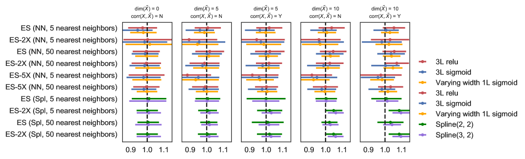
Figure 7: Performance of ES with different estimators for $\Sigma(X)^{-1}$ in the score expression

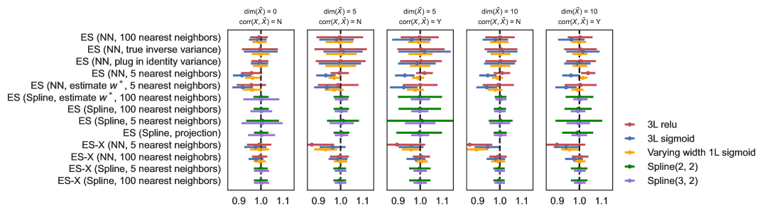
Figure 8: Performance of ES with different estimators for $\Sigma(X)^{-1}$ in the score expression

Below, we describe the procedures underlying Figure 2, which are representative of the procedures in Figures 1, 3 and 4. We also describe the procedures for Figures 5 and 6, which are in turn representative of the procedures in Figures 7, 8, 7 and 9.

Monte Carlo	Learning rate	# steps
1(b)	0.01	6000–10000
2	0.01	3000–5000
3(a)	0.01	7000–10000
3(b)	0.01	7000–10000
4	0.005	6000–10000
5	0.001	1500–2000

Table 1: Optimizer parameter choices for ANN SMD for $h$ for the NPIV designs. The number of steps is of the form (minimum number of steps)–(maximum number of steps), where an ad hoc stopping rule is used when the step size is in between, based on how much progress the optimization procedure is making. In our experience, in practice, the optimizer stops at near the minimum number of steps. We use PyTorch’s implementation of the Adam optimizer (torch.optim.Adam) throughout our experiments.

1. Figure 2 reports Monte Carlo means and standard deviations for the design in Monte Carlo design 2, using ANN SMD estimators under a variety of model specifications on true $h_{0}$.

   In particular, we make the following choices for estimation of various nuisance parameters.

   1. Identity-weighted SMD with simple plug-in: $\hat{\theta}_{\mathrm{SP}}\left({\hat{h}_{\mathrm{ISMD}}}\right)$ defined in Section 3.1. We specify choices of the linear sieve basis $\phi(\cdot)$ for instruments

      1. $\phi(X)=[\phi_{1}(X_{1},X_{2},X_{3}),\phi_{2}(X,\tilde{X})]$, where $\phi_{1}(X_{1},X_{2},X_{3})$ follows the basis choice made in Chen (2007) (p.5581–5582), and $\phi_{2}(X,\tilde{X})=[\tilde{X},\tilde{X}^{2},(X_{i}\tilde{X}_{j})_{i,j}]$ contains second-order polynomials for $\tilde{X}$ and interactions $X_{i}\tilde{X}_{j}$.

   2. Optimally-weighted SMD with orthogonalized plug-in: $\hat{\theta}_{\mathrm{OP}}\left({\hat{h}_{\mathrm{OSMD}},\hat{\Gamma}}\right)$ defined in Section 3.1. We specify estimation details for the nuisance functions $\Sigma(X),\Gamma(X)$:

      1. $\hat{\Sigma}(\cdot)$: Form the squared residuals from the identity-weighted estimator $v\equiv(y_{1}-\hat{h}_{\mathrm{ISMD}}(y_{2}))^{2}$ and estimate $\Sigma$ by $k=5$-nearest neighbors.

      2. $\hat{\Gamma}(\cdot)$: Given an estimate $\hat{\Sigma}$, it suffices to estimate

         $$\mathbb{E}[(\nabla_{1}h_{0}(Y_{2})-\theta_{0})(Y_{1}-h_{0}(Y_{2}))\mid X].$$

         Form $u\equiv\left[{\nabla_{1}\hat{h}_{\mathrm{OSMD}}(y_{2})-\hat{\theta}_{\mathrm{SP}}\left({\hat{h}_{\mathrm{ISMD}}}\right)}\right]\left({y_{1}-\hat{h}_{\mathrm{OSMD}}(y_{2})}\right)$ and project it on $\phi(X)$: i.e. $[\hat{\Gamma}(x_{1}),\ldots,\hat{\Gamma}(x_{n})]^{\prime}\equiv(P_{\phi}(\hat{\Sigma}^{-1}u))$.

   For Figure 2,

   1. The first column of Figure 2 reports results where the ANN SMD estimators are computed assuming $h_{0}$ is fully nonparametric.

   2. The second column of Figure 2 follows Section 3.4 in that we assume a partially linear structure on $h_{0}$, which is of the form $R_{1}\theta+h(R_{2},X_{2},\tilde{X})$.

   3. The third and the fourth columns of Figure 2 follow Section 3.4 in that we maintain the partially additive structure on $h_{0}$, which is of the form $R_{1}\theta+h_{1}(R_{2})+h_{2}(X_{2})+h_{3}(\tilde{X})$, where the unknown $h_{3}(\cdot)$ is approximated via ANNs. We use ANN sieves to approximate the scalar functions $h_{1},h_{2}$ in the 3rd column, whereas the fourth column uses spline sieves to approximate $h_{1},h_{2}$.

2. Figures 5 and 6 reports Monte Carlo means and standard deviations for a wide class of estimators (not limited to ANN SMD) for Monte Carlo design 2.

   1. ANN SMD: Follow Item 1 for Figure 2.

   2. Spline SMD:

      1. tensorLet $\lambda(x)$ be a spline basis for the instrument space of $X$, and let $\nu(y_{2})$ be a spline basis for the structural function $h(\cdot)$. Both $\lambda$ and $\nu$ are of the forms where each entry expands into a $\text{Spline}(k,2)$ basis, and pairwise interactions (of the form $x_{i}x_{j}$, but we do not include more complex interactions $f(x_{i})g(x_{j})$) are included in lieu of tensor product splines. The choice of order $k$ for $\lambda(x)$ is 1 more than that for $\nu(y_{2})$.

      2. Given $\lambda,\nu$, we estimate P-ISMD, OP-OSMD as in Item 1, where we optimize over candidate structural functions of the form $\nu(\cdot)^{\prime}\gamma$, and estimate $\Sigma$ and $\Gamma$ by least squares projections onto the instrument sieve $\lambda$.

   3. Score/influence function estimators: Let $\lambda(x),\nu(y_{2})$ be the spline bases used for the spline SMD in Item 2(b).

      1. IS:

         1. Estimate $\hat{h}_{\mathrm{ISMD}}$ as in Item 1(a) for ANN ISMD and as in Item 2(b) for spline ISMD.

         2. wstar$v^{\star}(y_{2})$ can be computed by solving (17). To do so, we approximate $w^{\star}(y_{2})$ with $\nu(y_{2})\beta$ for some coefficients $\beta$, and the $\mathbb{E}[\cdot\mid X]$ operator with $P_{\lambda}$. Doing so makes (17) a least-squares problem in the unknown coefficients $\beta$. In fact, the closed form solution is

            $$\hat{\beta}=-\left({\frac{1}{n}\nu(y_{2})^{\prime}P_{\lambda}\nu(y_{2})+\frac{1}{n^{2}}\nabla_{1}\nu(y_{2})11^{\prime}\nabla_{1}\nu(y_{2})}\right)^{-1}\left({\frac{1}{n}[\nabla_{1}\nu(y_{2})]^{\prime}1}\right),$$

            where $\nabla_{1}\nu(y_{2})\in\mathbb{R}^{n\times d_{\nu}}$ takes the partial derivative entry-wise. Therefore $\nu(y_{2})\hat{\beta}$ is the estimator for $w^{\star}$, and this gives an estimator for $v^{\star}$ by plugging in.

         3. Given $\hat{v}^{\star}(y_{2})$, we estimate $\kappa_{\mathrm{ID}}$ with $\hat{\kappa}_{\mathrm{ID}}(x)=P_{\lambda}\cdot\hat{v}^{\star}(y_{2})$.

         4. Plug $\hat{\kappa}_{\mathrm{ID}}(x)$ and $\hat{h}$ to the inefficient influence function and compute $\hat{\theta}_{\mathrm{IS}}$.

      2. ES:

         1. Estimate $\hat{h},\hat{\Gamma}$ as in Item 1(b) for ANN OSMD and as in Item 2(b) for spline OSMD.

         2. Estimate $v^{\star}$ by (20).

         3. Estimate $\Sigma$

         4. Form $\hat{\kappa}_{\mathrm{EIF}}(x)=\hat{\Gamma}(x)-P_{\lambda}[\hat{v}^{\star}(y_{2})]\hat{\Sigma}(x)^{-1}$, where $\Sigma$ estimated via $k(n)$-nearest neighbors, with $k(n)>5$.

         5. Plug $\hat{\kappa}_{\mathrm{EIF}}(x)$ and $\hat{h}$ to the efficient influence function and compute $\hat{\theta}_{\mathrm{ES}}$.

   4. AGMM: First we apply Dikkala et al. (2020)’s code to estimate structural function $h_{0}$ by $\hat{h}_{\mathrm{AGMM}}$. Then compute the simple plug-in $\hat{\theta}_{\mathrm{SP}}\left({\hat{h}_{\mathrm{AGMM}}}\right)$ defined in Section 3.1.

4.3 Monte Carlo Results

Due to the length of the paper, we report representative simulation results in a sequence of figures and tables below.

4.3.1 Performance of point estimates in terms of (Monte Carlo) bias and variance

condexpresultsFor Monte Carlo design 1(a), we compare the performance of a ReLU network (one hidden layer, 40 neurons) with the performance of a spline basis in Table 2. The performance metric we choose is the scaled integrated MSE:

$$R^{2}=1-\frac{\sum(\hat{f}(X_{i})-f(X_{i}))^{2}}{\min_{c}\sum(f(X_{i})-c)^{2}},$$

on 1000 out-of-sample data points. $R^{2}=1$ indicates perfect estimation of $f$, and $R^{2}=0$ indicates estimation quality on par with using a constant prediction. We find that for low and moderate noise, neural networks perform better than splines, presumably since it captures more complex interaction patterns in $f$. In the high noise regime, neural network underperforms, as neural networks overfit. In the very-high-noise regime, both estimators overfit and are in fact worse than simply using a constant. We caution that these performance of neural networks results from very minimal tuning, in particular, without validation samples. mcsimplediscNext, for Monte Carlo design 1(b), we show the results in Figure 1 for P-ISMD estimators, varying over the dimension $p$. We see that, despite the DGP involving a neural network, using neural network estimators only attains a modest improvement over spline estimators, in terms of slightly lower bias, consistent with our findings in the main text.

Table 2: Performance of ANN and spline for nonparametric regression

Noise-to-signal ratio	Spline $R^{2}$	Neural net $R^{2}$
0.0	0.60	0.91
0.1	0.58	0.80
1.0	0.48	0.30
10.0	-0.55	-2.55

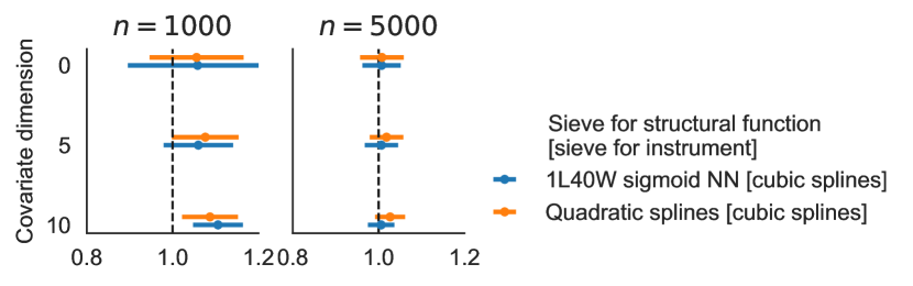
Figure 1: Performance of P-ISMD estimators on Monte Carlo design 1, where we vary over the dimension $p$ of the covariates $X$.

The rest of the figures correspond to more difficult Monte Carlo designs 2, 3 and 4 where the first element of $Y_{2}$ is endogenous ($R_{1}$). Figure 2 reports the performance of various ANN SMD estimators for $\theta$ in Monte Carlo design 2. The top display plots the results for $n=1000$ and the bottom for $n=5000$. Note here that the columns correspond to various assumptions we maintain on what the econometrician knows about the true structure of $h_{0}(.)$ in the model $\mathbb{E}[Y_{1}-h_{0}(Y_{2})|X]=0.$ The true design is partially additive, and the first column, NP, assumes that the econometrician has no knowledge of the true structure. As we can see, across all implementations (the rows), most of the ANN SMD estimators perform well, which indicates that ANNs seem able to adapt to the unknown structure of $h_{0}$. The second column labeled PL (for partially linear) assumes that $h_{0}(Y_{2})$ is partially linear (i.e., $h_{0}(Y_{2})=\theta R_{1}+h(R_{2},X_{2},\tilde{X})$) while the third column labeled PA assumes the correct additive structure (i.e., $h_{0}(Y_{2})=\theta R_{1}+h_{1}(R_{2})+h_{2}(X_{2})+h_{3}(\tilde{X})$) in the Monte Carlo design is known to the econometrician (but the functions $h_{1},h_{2},h_{3}$ within it are of course not known). PA column corresponds to the case where we use ANN sieves to learn all the unknown functions $h_{1},h_{2},h_{3}$ although $h_{1},h_{2}$ are functions of scalar random variable. Its performance slightly deteriorates as compared to the NP and PL columns. Notice here that for comparison, the last column for the PA case uses splines to approximate the two scalar valued unknown functions $h_{1}$ and $h_{2}$ while $h_{3}$ is always estimated via ANN (since it is of higher dimensions (at least when $\dim(\tilde{X})>0$). We see that the spline results are in line with the PL and NP results, and are adequate here.

In Figure 3, we report results for the various estimators for Monte Carlo design 3, where the unknown function $h_{0}$ is now nonlinear in the endogenous $R_{1}$ (the first element of $Y_{2}$). In the top panel (a), we report results for the case with $R^{2}/2$ and panel (b) reports results for the case where the unknown function is $R_{1}^{2}/2+R_{1}f(X_{2})$, where now the derivative depends on the regressor $X_{2}$ nonlinearly (as the function $f$ is highly nonlinear). Both results are for $n=1000,5000.$ For panel (a) we see that the spline estimator remain well behaved across all designs (across rows), the single-hidden layer (1L) sigmoid ANN estimators remain adequate while both versions of the AGMM estimators (Dikkala et al., 2020) exhibit some bias. In panel (b), spline remains well behaved and so are the ANN estimators. In Figure 4 we show estimates of the partial derivative evaluated at various fixed values for some regressors. Though the estimators do not track the function well, especially in the tails in the bottom display, the average derivative is estimated well. Interestingly, 3L relu ANN seems to estimate the derivative function marginally better than splines, perhaps since ANNs are able to automatically generate rich interaction behavior, whereas specifying tensor products for spline sieves is somewhat onerous.

We now examine various implementation choices for Monte Carlo design 2. In Figures 5 and 6, we compare various implementations of ANN estimators and spline estimators in Monte Carlo design 2. In Figure 5, we compare identity-weighted estimators (IS, P-ISMD, AGMM, IS-X). Note that P-ISMD and OP-OSMD are the plug in and optimal plug in SMD estimators. In Figure 6, we compare optimally-weighted estimators that are semiparametrically efficient under suitable regularity conditions (ES, OP-OSMD, ES-X). It is important at the outset to keep in mind that all ANN implementations require some non-negligible tuning as the optimization problem is non-convex and the problem itself with endogeneity, correlation among the regressors, and high dimensions is not easy to tune. Also, currently and for NPIV models, there is no theory for data driven approaches to picking width, depth, or activation functions and finite sample behavior in our design varied (For linear splines, there are data-driven choice of sieve terms, see Chen, Christensen and Kankanala, 2021a). The results across various combinations of $\dim(\tilde{X})$ and correlations for $n=1000,5000$ indicate first that ANN OP-OSMD and especially spline estimators seem to behave best. In particular, spline estimators require little tuning and are more stable than all ANN based estimators we use. The SMD ANN estimators are adequate with slight bias for the single-layer, varying-width case. IS and ES ANN estimators are generally less biased and slightly higher variance than P-ISMD and OP-OSMD ANN estimators, but we note that good performance of ES (in the ANN case) is very sensitive to the choice of $\hat{\Sigma}(X)^{-1}$ in the “optimally-weighted” Riesz representer estimation. Figures 7 and 8 compare the performances of ES in a variety of choices for $\hat{\Sigma}(X)$. It is interesting that the poor choice of $\hat{\Sigma}(X)^{-1}$ leads to biased estimation of ES and its cross-fitted versions.

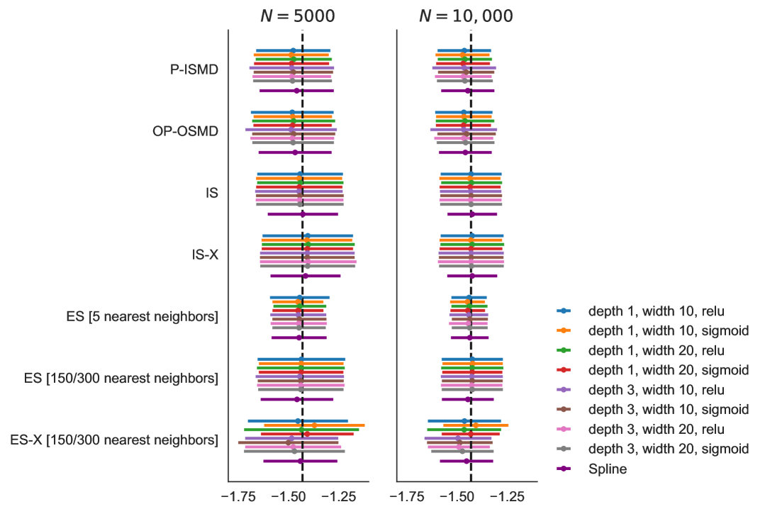
Figure 9: Performance of various estimators in Monte Carlo design 4 across two sample sizes

calibrateddiscLastly, Figure 9 examines various estimators on the empirical calibration Monte Carlo design 4. Consistent with the findings in other Monte Carlo settings, we generally find that all estimators perform adequately, with similar performance across a variety of neural architectures. We also continue to find that SMD estimators P-ISMD , OP-OSMD have slightly better mean-squared error performance than the score-based estimators in exchange for slightly higher bias. The one exception is ES with variance estimation with only five nearest neighbors, which performs best across the specifications. We conjecture that this is due to how we constructed the residuals in Monte Carlo design 4. In particular, we multiply standard Gaussians with estimated residuals $R_{i}^{P},R_{i}^{Y}$, which may result in a conditional variance function that is highly non-smooth, and, as a result, a low number of nearest neighbor estimates performs well. In any case, the performance of ES and ES-X continues to show that it is sensitive to $\hat{\Sigma}(X)$, as is shown in Figures 7 and 8.

See Appendix A for additional Monte Carlo results.

4.3.2 Performance of inference statistics

Tables 6 and 7 provides various inference statistics for the ANN SMD estimators P-ISMD and OP-OSMD for Monte Carlo design 2, without assuming any semiparametric structure on $h(\cdot)$ beyond smoothness. In particular, we report bootstrapped confidence intervals for ReLU and sigmoid and for depths 1 and 3 when the dimension of the nuisance variables $\tilde{X}$ ranges from 0 to 10. The results are also given for sample sizes $n=1000$ and $n=5000.$ Across all specifications, the two ANN estimators perform adequately.

In Figure 10, we examine various standard error approaches for a set of estimators in Monte Carlo design 2. For each of these, we compute the MC standard deviation, a feasible estimator based on the estimator variance derived from theory, and a bootstrapped standard error. Overall, the theory and bootstrapped standard errors are adequate. In unreported results, criterion (SMD) based bootstrap confidence intervals showed reasonable coverage performance.

4.3.3 Overall simulation findings

Overall, it seems that ANN methods are useful in approximating potentially high dimensional functions in NPIV models. Also, in the class of models we investigated, choices of layers, widths or activation functions are not very consequential in terms of finite sample performance. On the other hand, ANN based estimators in these non-standard NPIV models are hard to tune, and a researcher needs to choose many smoothing parameters. These ANN estimators are also unstable in some runs as they are based on highly complex (and non-convex) optimization programs. In addition, ANNs are not as effective in estimating univariate functions. Finally, to our surprise, We find that various plug-in spline SMD estimators appear stable, less biased generally and can outperform ANNs for NPIV models even in high dimensional cases with 13 continuous regressors.

5 Empirical Illustrations

We present two empirical applications of estimating average derivatives with respect to endogenous price of a nonparametric demand $h_{0}(Y_{2})$ for some non-durable goods. We apply ANN sieves to approximate $h_{0}(\cdot)$ nonparametrically when its argument $Y_{2}$ consists of 7 covariates (for gasoline demand) and 6 covariates (for strawberry demand). In the existing literature researchers have used both data sets to estimate unknown $h_{0}(\cdot)$ in the model $\mathbb{E}[Y_{1}-h_{0}(Y_{2})\mid X]=0$ by assuming $h$ takes some parametric or semiparametric (such as partially linear) form to avoid the “curse of dimensionality” of $Y_{2}$. Although served as illustrations, our applications below are the first to estimate the endogenous demand function $h_{0}(\cdot)$ fully nonparametrically when $\dim(Y_{2})>5$.

5.1 Gasoline demand

We use data on gasoline demand from the 2001 National Household Travel Survey (Blundell, Horowitz and Parey, 2012). The sample we use include 4,812 observations in the full sample as in Chen and Christensen (2018). We estimate an NPIV analogue of the model (11) in Blundell, Horowitz and Parey (2012), $\mathbb{E}[Y_{1}-h_{0}(Y_{2})\mid X]=0$ where $Y_{1}$ is the log gasoline demand, and $Y_{2}$ is a vector of 7 random variables consisting of the log gasoline price (possibly endogenous) and the other included covariates following Column (3) in Table 2 of Blundell, Horowitz and Parey (2012). The instrument is the distance from the Gulf coast. We define the estimand as the average price derivative of the unknown structural function $h_{0}(\cdot)$, which has an average elasticity interpretation. blundell2012measuring via OLS, and

Table 3: Estimates of price elasticity for gasoline in National Household Travel Survey data (Blundell, Horowitz and Parey, 2012)

	P-ISMD	OP-OSMD	IS
Sigmoid [1L]	-1.28	-1.24	-1.12
	[-1.69, -0.9]	[-1.64, -0.87]	(0.22)
Sigmoid [3L]	-1.24	-1.28	-1.11
	[-1.65, -0.9]	[-1.64, -0.87]	(0.22)
ReLU [3L]	-1.27	-1.25	-1.14
	[-1.65, -0.9]	[-1.64, -0.87]	(0.22)
Spline(3, 2)	-1.17	-1.2
	[-1.57, -0.8]	[-1.6,-0.8]
	Blundell et al. (2012) OLS	OLS	TSLS
	-0.83	-0.85	-1.24
	(0.148)	(0.15)	(0.2)

Notes.

The 7 included covariates ($Y_{2}$) are: log gasoline price, log income, household size, driver, household age, number working, public transit distance. We instrument gasoline price with distance to Gulf of Mexico. ∎

Table 3 shows our estimates for the average price elasticity (and bootstrapped $95\%$ confidence intervals). Broadly speaking, these estimates point to a similar range of values and are similar to a parametric two-stage least-squares specification. Across estimator classes, the ANN SMD estimates are slightly larger in magnitude than the spline SMD estimates and the ANN IS estimates. Within the ANN SMD estimator class, architecture choices of the networks do not appear to matter much for the result.

5.2 Strawberry demand

Table 4: Estimate of demand average derivatives from Nielsen strawberry demand data (Compiani, 2019)

Non-organic

	IS	P-ISMD	OP-OSMD
Sigm [1L]	-1.649	-1.530	-1.747
	(0.04)	(0.04)	(0.03)
		[-1.8, -1.7]	[-2.3, -1.8]
Relu [1L]	-1.648	-1.590	-1.706
	(0.04)	(0.04)	(0.04)
		[-1.9, -1.7]	[-2.3, -1.8]
Relu [3L]	-1.648	-1.634	-1.659
	(0.04)	(0.04)	(0.06)
		[-1.9, -1.55]	[-2.2, -1.5]
Spline(3,2)	-1.611	-1.648	-1.676
	(0.04)	(0.04)	(0.04)

Organic

	IS	P-ISMD	OP-OSMD
Sigm [1L]	-3.235	-2.409	-3.382
	(0.07)	(0.09)	(0.06)
		[-2.7, -2.44]	[-4.3, -3.5]
Relu [1L]	-3.236	-2.197	-2.129
	(0.07)	(0.06)	(0.08)
		[-2.4, -2.11]	[-2.4, -2.06]
Relu [3L]	-3.232	-2.206	-2.122
	(0.07)	(0.07)	(0.14)
		[-3.1, -2.08]	[-2.36, -2.06]
Spline(3,2)	-3.194	-3.232	-3.124
	(0.06)	(0.07)	(0.06)

Notes.

The 6 included covariates ($Y_{2}$) are: strawberry prices (non-organic, organic), income, lettuce demand (taste for organic proxy), state-level sale of non-strawberry fresh fruits, average outside good price. The excluded instruments are 3 Hausman IV (prices in neighbouring markets)+ 2 strawberry spot prices (marginal cost measures). A market is defined at the store-week level and there are $N=38,800$ markets. ∎

We also consider a setting where consumers choose two substitutable goods. We use the Nielsen dataset from Compiani (2019), where consumers in California choose from strawberries, organic strawberries, and an outside option. We observe the market share of each type of product, their prices, and a variety of covariates at the market (store-week) level. In the analysis, we consider NPIV model $\mathbb{E}[Y_{1}-h_{0}(Y_{2})\mid X]=0$ where $Y_{1}$ is the log market share of a type of good (non-organic or organic strawberries) and $Y_{2}$ is a vector of 6 random variables, including endogenous prices for both types of strawberries and the outside good, and other market-level covariates. The instruments $X$ include Hausman instruments as well as cost shifters such as measurements of consumer taste and income at the market level. We focus on the target parameter $\theta_{0}=\mathbb{E}[\nabla_{1}h_{0}]$, which is the average derivative of $h$ with respect to the own-price in logs, which we interpret as a version of price elasticity.

We present the results in Table 4. As is perhaps expected from a casual intuition, estimates of $\theta_{0}$ are negative across both products, and more negative for the more price-sensitive product (organic strawberry). Moreover, results are broadly similar across estimation methods (SMD vs. score) and sieve choices (spline vs. neural net), with perhaps more variability for neural networks in organic strawberries. The estimates for non-organic strawberries hover around $-1.5$, and are reasonably stable across choices of tuning parameters and estimators (IS vs. SMD estimators). The estimates for organic strawberries are more variable across specification of nuisance parameters and neural architectures, but seem to be around $-2$ and $-3$, and larger in magnitude than the own-price elasticity estimate for non-organic strawberries.

These estimates are qualitatively similar to Compiani (2019)’s estimates, which reports median own-price elasticities of $-1.4$ (0.03) for non-organic strawberries and $-5.5$ (0.7) for organic strawberries. Our estimates are more dissimilar for organic strawberries, for which we offer a few conjectures. First, Compiani (2019) reports estimates following Berry and Haile (2016)’s approach to demand estimation, that accounts for price endogeneity differently. Under his assumptions, it is possible that our estimator is consistent for a different parameter than his. Second, organic strawberry market shares are very small, and hence fluctuates more on a log scale, thereby resulting in worse estimation precision.

6 Conclusion

conc In this paper, we present two classes of semiparametric efficient estimators for weighted average derivatives (WADs) of nonparametric instrumental variables regressions (NPIV) of moderate and high dimensional endogenous and exogenous regressors. We have conducted detailed Monte Carlo comparisons of finite sample performance of various inefficient and efficient estimators of the WADs using various ANN sieves. The simulation studies and empirical applications confirm the theoretical advantage of ANN approximation of unknown continuous functions of moderately high-dimensional variables, after some tuning of hyper-parameters. Perhaps the most practical findings from our large amount of reported and unreported simulation studies using moderate sample sizes are as follows: the ANN efficient SMD estimators have smaller biases than those of the ANN inefficient SMD estimators, and are less sensitive to the tuning parameters than those of the ANN efficient score estimators. In addition, simple spline based estimators of WADs of NPIVs perform very well in terms of finite sample biases and variances. More research is needed to close the gap between approximation theory and finite sample computational performance in applying flexible ANNs to nonparametric models with endogeneity.

Figure 2: ANN SMD estimators for Monte Carlo design 2

(a) $n=1000$

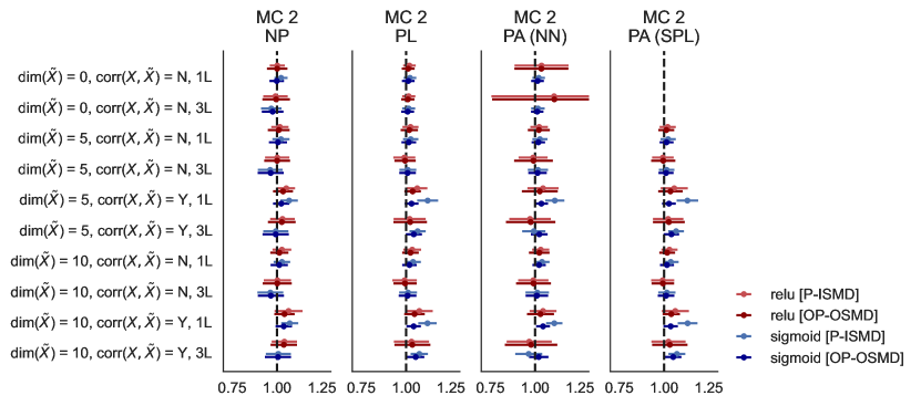
(b) $n=5000$

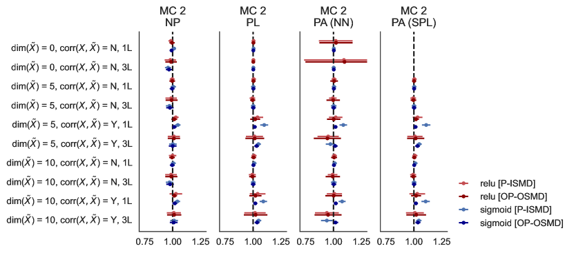
Notes.

Monte Carlo Mean $\pm 1$ Monte Carlo standard deviation across 1,000 replications.

The columns are estimators where different correct assumptions of the data-generating process are placed. The first column (NP: nonparametric) shows estimated average derivative of an NPIV model, where the unknown function $h(Y_{2})$ is not assumed to have separable structure. The second column (PL: partially linear) assumes $h(Y_{2})=\theta R_{1}+h_{1}(R_{2},X_{2},\tilde{X})$. The third and fourth columns (PA: partially additive) assumes $h(Y_{2})=\theta R_{1}+h_{1}(R_{2})+h_{2}(X_{2})+h_{3}(\tilde{X})$. The third column uses neural networks to approximate the scalar functions $h_{1},h_{2}$, and the fourth column uses splines to approximate $h_{1},h_{2}$ (while $h_{3}$ is always estimated via ANN).

For each type of assumption placed on the true $h_{0}(Y_{2})$, we vary the data-generating process by varying the dimension of $\tilde{X}$ and the level of correlation between $(X_{1},X_{2},X_{3})$ and $\tilde{X}$. We also vary the network architecture by $\{\text{ReLU},\text{Sigmoid}\}\times\{\text{1L, 3L}\}\times\{\text{10W}\}.$ Lastly, we vary the type of estimator used from simple plug-in with the identity-weighted SMD estimator to orthogonalized plug-in with the optimally-weighted SMD estimator. ∎

Figure 3: Estimation quality of average derivative parameter in Monte Carlo design 3 across a variety of NPIV estimators

(a) Monte Carlo design 3(a)

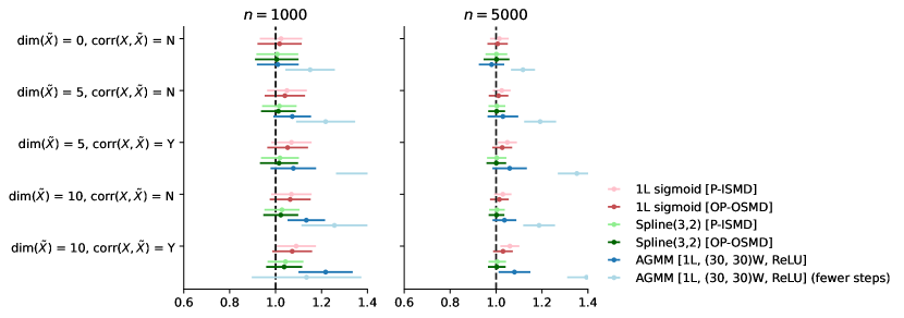
(b) Monte Carlo design 3(b)

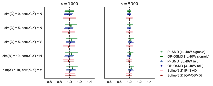
Figure 4: Estimation quality of the partial derivative function in Monte Carlo design 3(b) across a variety of estimators

(a) Estimated $f_{1}$ versus true $f_{1}$. Single sample for $N=5,000$

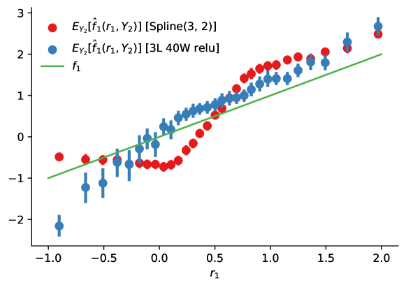
(b) Estimated $f_{2}$ versus true $f_{2}$. Single sample for $N=5,000$

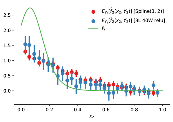
Notes.

In the DGP Monte Carlo design 3(b), the partial derivative $\nabla_{1}h_{0}$ is of the form $f_{1}(R_{2})+f_{2}(X_{2})$, and we evaluate performance estimating $f_{1},f_{2}$. Estimated $f_{1}$ is calculated by taking $\nabla_{1}\hat{h}-f_{2}(x_{2})$. We plot expectation marginalizing over variables other than $r_{1}$. Estimated $f_{2}$ is calculated by taking $\nabla_{1}\hat{h}-f_{1}(r_{1})$. We plot expectation marginalizing over variables other than $x_{2}$. Both estimators use the same instrument basis. ∎

Figure 5: Estimation quality of average derivative parameter in Monte Carlo design 2 across a variety of identity-weighted estimators

(a) Monte Carlo design 2, Nonparametric, $n=1000$

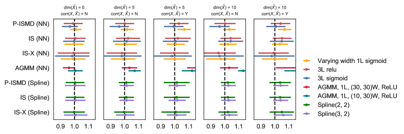
(b) Monte Carlo design 2, Nonparametric, $n=5000$

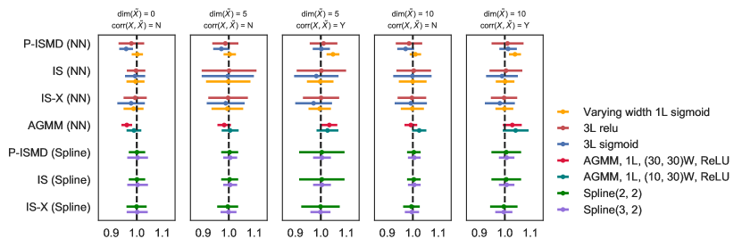
Notes.

Monte Carlo Mean $\pm 1$ Monte Carlo standard deviation across 1,000 replications.

We consider a few different estimation strategies and vary over choice of tuning parameters for nuisance parameters in these estimation strategies.

In terms of estimation strategies, IS stands for identity score estimators, detailed in Item 2, whereas IS-X stands for the score estimators, but with two-fold cross-fitting. AGMM uses the adversarial GMM estimation algorithm in Dikkala et al. (2020) to compute $\hat{h}$, and outputs the simple plug-in estimator for $\theta$. P-ISMD estimators follow Item 1.

In terms of neural architecture and spline parameter choices, varying width 1L sigmoid refers to using 1-layer sigmoid network, but vary the width of the network according to $\dim(\tilde{X})$, as opposed to fixing the width at 10. The two AGMM architecture choices refer to different widths for the network estimating $h$ and the adversarial network approximating the instrument test functions, where (10,30)W refers to using width-10 for $h$ and width-30 for the instruments. Lastly, $\text{Spline}(a,b)$ is a spline basis for approximating $h$ such that each spline function is an $(a-1)$-degree piecewise polynomial that have $b$ knots, where we include pairwise interactions in lieu of tensor products. In the spline scenarios, $\text{Spline}(a+1,b)$ is used as a spline basis for the instruments. Tuning parameter choices for estimation of additional nuisance parameters are detailed in Table 5. ∎

Figure 6: Estimation quality of average derivative parameter in Monte Carlo design 2 across a variety of optimally weighted estimators

(a) Monte Carlo design 2, Nonparametric, $n=1000$

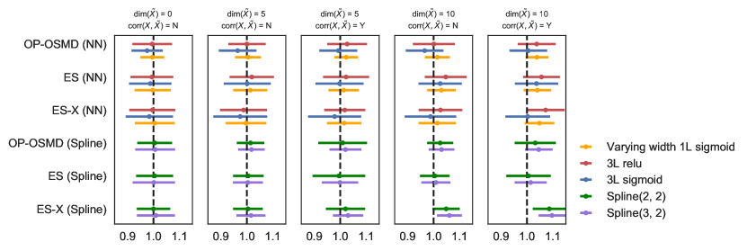
(b) Monte Carlo design 2, Nonparametric, $n=5000$

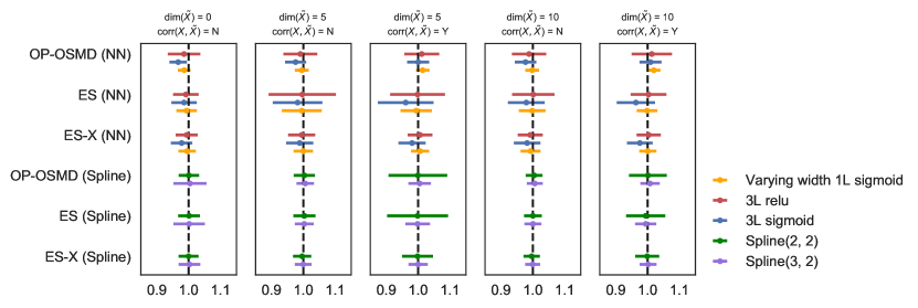
Notes.

Monte Carlo Mean $\pm 1$ Monte Carlo standard deviation across 1,000 replications.

We consider a few different estimation strategies and vary over choice of tuning parameters for nuisance parameters in these estimation strategies.

In terms of estimation strategies, ES stands for efficient score estimators, detailed in Item 2, whereas ES-X stands for the score estimators, but with two-fold cross-fitting. OP-OSMD estimators follow Item 1.

In terms of neural architecture and spline parameter choices, varying width 1L sigmoid refers to using 1-layer sigmoid network, but vary the width of the network according to $\dim(\tilde{X})$, as opposed to fixing the width at 10. Lastly, $\text{Spline}(a,b)$ is a spline basis for approximating $h$ such that each spline function is an $(a-1)$-degree piecewise polynomial that have $b$ knots, where we include pairwise interactions in lieu of tensor products. In the spline scenarios, $\text{Spline}(a+1,b)$ is used as a spline basis for the instruments. Tuning parameter choices for estimation of additional nuisance parameters are detailed in Table 5. ∎

$n=1000$

Notes.

Monte Carlo Mean $\pm 1$ Monte Carlo standard deviation across 1,000 replications.

“$k$-nearest neighbors”: Use $k$-nearest neighbors to estimate $\Sigma(X)$ in the score (in $\mathbb{E}[v^{\star}\mid X]\Sigma(X)^{-1}$).

“True inverse variance”: Plug in the true $\Sigma(X)$ for that in the score.

“Plug in identity”: Plug in the identity matrix for $\Sigma(X)$ in the score.

“Projection”: Use the projection of the squared residuals onto spline bases for $\Sigma(X)$.

“Estimate $w^{\star}$”: Instead of estimating $v^{\star}$ with sieves, we estimate $w^{\star}$ with sieves and form $v^{\star}$ via plugging in estimates of other nuisance parameters. ∎

$n=5000$

Notes.

Monte Carlo Mean $\pm 1$ Monte Carlo standard deviation across 1,000 replications.

“$k$-nearest neighbors”: Use $k$-nearest neighbors to estimate $\Sigma(X)$ in the score (in $\mathbb{E}[v^{\star}\mid X]\Sigma(X)^{-1}$).

“True inverse variance”: Plug in the true $\Sigma(X)$ for that in the score.

“Plug in identity”: Plug in the identity matrix for $\Sigma(X)$ in the score.

“Projection”: Use the projection of the squared residuals onto spline bases for $\Sigma(X)$.

“Estimate $w^{\star}$”: Instead of estimating $v^{\star}$ with sieves, we estimate $w^{\star}$ with sieves and form $v^{\star}$ via plugging in estimates of other nuisance parameters. ∎

Notes.

Monte Carlo Mean $\pm 1$ Monte Carlo standard deviation across 1,000 replications.

“150/300 nearest neighbors”: 150 nearest neighbors for $N=5000$, 300 nearest neighbors for $N=10000$ in estimating $\hat{\Sigma}(X)$.

Splines use two knot cubic splines for instrument basis, and two knot quadratic splines for endogenous functions. ∎

Estimator type	$\Sigma(X)$ [SMD]	$\Gamma(X)$	$\Sigma(X)$ [Score]	$v^{\star}$ [Score]
P-ISMD [NN]
OP-OSMD [NN]	5 nearest neighbors	Projection of demeaned $(\nabla\hat{h}-\overline{\nabla\hat{h}})((y-\hat{h})-\overline{(y-\hat{h})})$ on instrument basis ($\phi$) used in SMD estimation. Then multiply $\Sigma(X)^{-1}$ estimate for SMD. Project the result onto the sieve basis for the instruments.
IS [NN]				Sieve calculation of (17) with Spline(3, 2) ($\lambda$)
ES [NN]	Same as OP-OSMD [NN]	Same as OP-OSMD [NN]	50 nearest neighbors for $n=1000$, 100 for $n=5000$	Sieve calculation of (20) with Spline(3, 2) ($\lambda$)
IS/ES-X [NN]	Both scores take the form of $\nabla\hat{h}-\lambda(x)^{\prime}\hat{\xi}\cdot(y-\hat{h})$ where $\lambda(x)$ is a sieve basis (Spline(3, 2)). The sample is split so that $\hat{h}$ and $\hat{\xi}$ are estimated from one half and the score is computed on the other. The roles of the two subsamples are then exchanged.
P-ISMD [Spl]
OP-OSMD [Spl]	Projection onto sieve basis $(\lambda)$ for the instruments	Projection of demeaned $(\nabla\hat{h}-\overline{\nabla\hat{h}})((y-\hat{h})-\overline{(y-\hat{h})})$ on instrument basis ($\lambda$) used in SMD estimation. Then multiply $\Sigma(X)^{-1}$ estimate from SMD. Project the result onto the sieve basis for the instruments.
IS [Spl]				Sieve calculation of (17) with same spline basis ($\lambda$) as the instruments
ES [Spl]	Same as OP-OSMD [Spl]	Same as OP-OSMD [Spl]	50 nearest neighbors for $n=1000$, 100 for $n=5000$	Sieve calculation of (20) with same spline basis ($\lambda$) as the instruments
IS/ES-X [Spl]	Both scores take the form of $\nu(y_{2})^{\prime}\hat{\beta}-\lambda(x)^{\prime}\hat{\xi}\cdot(y-\hat{h})$ where $\lambda(x),\nu(y_{2})$ are sieve bases. The sample is split so that $\hat{\beta}$ and $\hat{\xi}$ are estimated from one half and the score is computed on the other. The roles of the two subsamples are then exchanged.

Table 5: Estimation of additional nuisance parameters

Table 6: SMD inference results for P-ISMD and OP-OSMD average derivative parameter in Monte Carlo design 2, $n=1000$

				P-ISMD					OP-OSMD
				Mean	Std	Med. Est. SE	Boot. LB	Boot. UB	Mean	Std	Med. Est. SE	Boot. LB	Boot. UB
Nui. Dim	Corr($X,\tilde{X}$)	Depth	Activation
0	0.0000	1	relu	1.001	0.042	0.045	0.948	1.077	1.001	0.057	0.029	0.909	1.102
			sigmoid	1.022	0.036	0.046	0.978	1.118	0.998	0.040	0.026	0.913	1.108
		3	relu	0.991	0.068	0.053	0.913	1.087	0.995	0.076	0.033	0.840	1.235
			sigmoid	0.968	0.057	0.069	0.871	1.107	0.975	0.060	0.043	0.883	1.126
5	0.0000	1	relu	1.016	0.048	0.054	0.889	1.200	1.009	0.061	0.040	0.870	1.218
			sigmoid	1.022	0.048	0.057	0.873	1.103	1.005	0.050	0.037	0.893	1.133
		3	relu	1.001	0.068	0.061	0.878	1.085	1.000	0.072	0.043	0.875	1.096
			sigmoid	0.962	0.069	0.088	0.713	1.024	0.964	0.072	0.061	0.722	1.048
	0.5000	1	relu	1.052	0.049	0.052	0.946	1.159	1.033	0.055	0.038	0.906	1.142
			sigmoid	1.067	0.048	0.053	0.921	1.163	1.023	0.046	0.035	0.904	1.116
		3	relu	1.030	0.068	0.060	0.895	1.143	1.026	0.077	0.043	0.905	1.167
			sigmoid	0.993	0.070	0.090	0.740	1.054	0.992	0.073	0.062	0.722	1.072
10	0.0000	1	relu	1.027	0.052	0.061	0.915	1.090	1.013	0.051	0.045	0.908	1.104
			sigmoid	1.027	0.046	0.062	0.900	1.111	1.012	0.048	0.042	0.940	1.157
		3	relu	1.002	0.076	0.070	0.749	1.179	1.001	0.081	0.052	0.753	1.184
			sigmoid	0.963	0.072	0.101	0.670	1.015	0.965	0.073	0.072	0.682	1.026
	0.5000	1	relu	1.064	0.078	0.064	0.968	1.147	1.041	0.057	0.045	0.959	1.148
			sigmoid	1.071	0.047	0.064	0.931	1.133	1.037	0.046	0.044	0.935	1.135
		3	relu	1.041	0.070	0.073	0.865	1.251	1.038	0.073	0.052	0.867	1.278
			sigmoid	1.007	0.070	0.105	0.749	1.041	1.005	0.073	0.075	0.740	1.056

Notes.

1000 Monte Carlo replications. Bootstrap CIs based on a single replication. ∎

Table 7: SMD inference results for P-ISMD and OP-OSMD average derivative parameter in Monte Carlo design 2, $n=5000$

				P-ISMD					OP-OSMD
				Mean	Std	Med. Est. SE	Boot. LB	Boot. UB	Mean	Std	Med. Est. SE	Boot. LB	Boot. UB
Nui. Dim	Corr($X,\tilde{X}$)	Depth	Activation
0	0.0000	1	relu	0.985	0.022	0.021	0.966	1.036	0.994	0.023	0.013	0.897	1.031
			sigmoid	1.013	0.018	0.021	0.976	1.054	0.990	0.018	0.011	0.942	1.026
		3	relu	0.979	0.050	0.023	0.933	1.012	0.986	0.051	0.014	0.850	1.056
			sigmoid	0.958	0.027	0.033	0.876	0.978	0.967	0.027	0.021	0.881	1.035
5	0.0000	1	relu	0.996	0.022	0.024	0.968	1.079	0.997	0.025	0.017	0.912	1.076
			sigmoid	1.006	0.024	0.025	0.964	1.065	0.995	0.022	0.015	0.940	1.034
		3	relu	0.986	0.051	0.026	0.922	1.041	0.990	0.053	0.018	0.914	1.043
			sigmoid	0.971	0.032	0.037	0.938	1.071	0.976	0.033	0.024	0.933	1.078
	0.5000	1	relu	1.028	0.025	0.023	0.976	1.071	1.014	0.025	0.016	0.907	1.052
			sigmoid	1.046	0.024	0.022	1.002	1.117	1.014	0.021	0.014	0.960	1.049
		3	relu	1.011	0.054	0.025	0.942	1.045	1.011	0.055	0.018	0.923	1.038
			sigmoid	1.002	0.033	0.037	0.927	1.066	1.000	0.034	0.025	0.908	1.060
10	0.0000	1	relu	0.999	0.033	0.025	0.959	1.044	0.994	0.025	0.018	0.933	1.031
			sigmoid	1.005	0.022	0.025	0.969	1.064	0.997	0.022	0.016	0.936	1.032
		3	relu	0.985	0.052	0.027	0.848	1.050	0.988	0.054	0.019	0.848	1.055
			sigmoid	0.972	0.033	0.039	0.930	1.064	0.977	0.034	0.027	0.932	1.068
	0.5000	1	relu	1.029	0.056	0.025	0.981	1.065	1.016	0.023	0.018	0.956	1.047
			sigmoid	1.042	0.025	0.024	1.008	1.113	1.020	0.021	0.016	0.973	1.065
		3	relu	1.010	0.062	0.028	0.911	1.126	1.013	0.063	0.020	0.901	1.122
			sigmoid	1.013	0.034	0.041	0.937	1.073	1.009	0.035	0.028	0.927	1.065

Notes.

1000 Monte Carlo replications. Bootstrap CIs based on a single replication. ∎

Figure 10: Inference quality of average derivatrive parameter in Monte Carlo design 2 across a variety of estimators

(a) Monte Carlo design 2, Nonparametric, $n=1000$

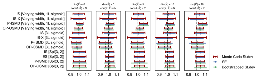
(b) Monte Carlo design 2, Nonparametric, $n=5000$

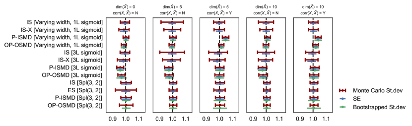
Notes.

Monte Carlo Mean $\pm 1\{\text{Monte Carlo st. dev., estimated s.e., bootstrapped s.e.}\}$ across 1,000 replications.

Bootstrap SEs are based on one realization of the data. ∎

Appendix A Appendix: Additional Monte Carlo Results

An additional Monte Carlo and sensitivity to instrument basis.

Monte Carlo design 5.

This is an augmentation of the design in Chen (2007). This design has a simpler functional form of $h_{0}$:

$$Y_{1}=h_{0}(Y_{2})+U=X_{1}+h_{01}(R)+h_{02}(X_{2})+h_{03}(\tilde{X})+U,\quad\mathbb{E}[U\mid X_{1},X_{2},X_{3},\tilde{X}]=0,$$

where we generate

$$h_{01}:\mathbb{R}\to\mathbb{R} \quad t\mapsto\frac{1}{1+\exp(-t)}$$

$$h_{02}(t):\mathbb{R}\to\mathbb{R} \quad t\mapsto\log(1+t)$$

$$h_{03}:\mathbb{R}^{d_{\tilde{x}}}\to\mathbb{R} \quad\tilde{x}\mapsto 5\tilde{x}_{1}^{3}+\tilde{x}_{2}\cdot\max_{j=1,\ldots,d_{\tilde{x}}}\left({\tilde{x}_{j}\vee 0.5}\right)+0.5\exp(-\tilde{x}_{d_{\tilde{x}}})$$

$$X_{1},X_{2},X_{3} \sim\operatorname{Unif}[0,1]$$

$$U\mid X_{1},X_{2},X_{3} \sim\mathcal{N}\left({0,\frac{1}{3}(X_{1}^{2}+X_{2}^{2}+X_{3}^{2})}\right)$$

$$\epsilon \sim\mathcal{N}(0,0.1)$$

$$R =X_{1}+X_{2}+X_{3}+0.9U+\epsilon.$$

The process generating $\tilde{X}$ is somewhat complex. First, we generate a covariance matrix $\Sigma\propto(I+Z^{\prime}Z)$, normalized to unit diagonals, where $Z$’s entries are i.i.d. standard Normal. The seed generating the covariance matrix is held fixed over different samples, and so $\Sigma$ should be viewed as fixed a priori. Next, let $\rho\in[-1,1]$ denote a correlation level and we let

$$\tilde{X}=\Phi\left({\rho(X_{1}+X_{2}+X_{3})+\sqrt{1-\rho^{2}}T}\right)\quad T\sim\mathcal{N}(0,\Sigma),$$ (22)

where $\Phi(\cdot)$ is the standard Normal CDF, and $\Phi(\cdot)$ and addition are applied elementwise. In the exercises reported, we use $\rho\in\{0,0.5\}$ for correlation levels. This Monte Carlo design becomes identical to the one used in Chen (2007) when $\tilde{X}$ is an empty vector. We increase the dimension of $\tilde{X}$ to $5$ and $10$ to make the estimation problem more difficult. Note that this design allows for correlation among regressors both endogenous and exogenous. It also allows for heteroskedasticity and possibly large dimensions by increasing the dimension of $\tilde{X}$. We have also tried different conditional variance of $U$, the simulation results are similar.

To connect with the notation in the previous sections, let $Y_{2}=[X_{1},R,X_{2},\tilde{X}]$ and $X=[X_{1},X_{2},X_{3},\tilde{X}]$. The parameter of interest is $\theta_{0}=\mathbb{E}\left[{\frac{\partial{h_{0}(Y_{2})}}{\partial{X_{1}}}}\right]=1$.

The estimation choices for Monte Carlo design 5 are exactly as in Item 1. Figure 11 plots the performance of various ANN SMD estimators in terms of mean $\pm$ one (Monte Carlo) standard deviation across 1000 replications for Monte Carlo design 5, in which the first element of $Y_{2}$ is exogenous ($X_{1}$). As a reminder, P-ISMD is the simple plug in estimator of $\theta$ with identity weighting, while OP-OSMD is the orthogonalized plug in with optimal weighting for the SMD objective. As we can see across layers and activation function, and whether we have a low dimensional regime in the left hand side columns or large dimensional regimes in the right hand columns, or whether there is correlation across regressors (denoted by Y(es) or N(o) on top of each column), the behavior of these ANN estimators is similar and adequate. All the intervals are more or less centered on top of the truth, $\theta_{0}=1$, while the efficient estimator OP-OSMD is slightly less biased.

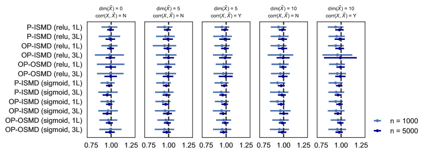
Figure 11: ANN SMD estimators for the average derivative parameter in Monte Carlo design 5

Notes.

Monte Carlo Mean $\pm 1$ Monte Carlo standard deviation across 1,000 replications. ∎

Figures 12 and 13 are replicates of Figures 11 and 2 respectively, except for slightly smaller instrument sieve bases. Specifically, we only use $\phi_{1}$ in item 1(a)i in Section 4.2 as the basis, as opposed to using both $\phi_{1},\phi_{2}$. We see that the ANN SMD estimates for the simpler Monte Carlo design 5 are not sensitive to the choice of instrument sieves, while the ANN SMD estimates for Monte Carlo design 2 are slightly more sensitive to the choice of instrument sieves.

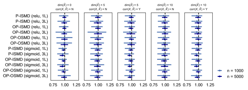
Figure 12: ANN SMD estimators for Monte Carlo design 5 with smaller instrument basis

Notes.

Monte Carlo Mean $\pm 1$ Monte Carlo standard deviation across 1,000 replications.

∎

Figure 13: ANN SMD estimators for Monte Carlo design 2 with smaller instrument basis

(a) $n=1000$ (Smaller instrument basis)

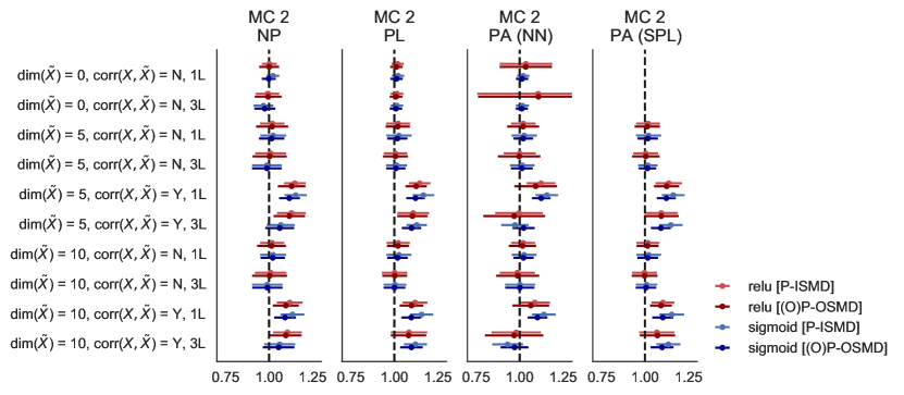
(b) $n=5000$ (Smaller instrument basis)

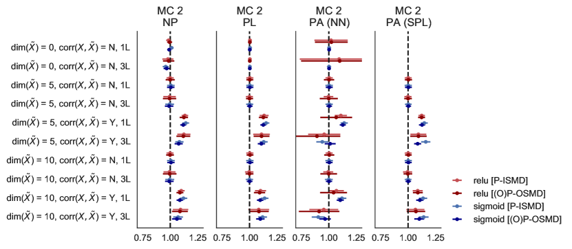
Notes.

Monte Carlo Mean $\pm 1$ Monte Carlo standard deviation across 1,000 replications.

The columns are estimators where different correct assumptions of the data-generating process are placed. The first column (NP: nonparametric) shows estimated average derivative of an NPIV model, where the unknown function $h(Y_{2})$ is not assumed to have separable structure. The second column (PL: partially linear) assumes $h(Y_{2})=\theta R_{1}+h_{1}(R_{2},X_{2},\tilde{X})$. The third and fourth columns (PA: partially additive) assumes $h(Y_{2})=\theta R_{1}+h_{1}(R_{2})+h_{2}(X_{2})+h_{3}(\tilde{X})$. The third column uses neural networks to approximate the scalar functions $h_{1},h_{2}$, and the fourth column uses splines to approximate $h_{1},h_{2}$.

For each type of assumption placed on the true $h_{0}(Y_{2})$, we vary the data-generating process by varying the dimension of $\tilde{X}$ and the level of correlation between $(X_{1},X_{2},X_{3})$ and $\tilde{X}$. We also vary the network architecture by $\{\text{ReLU},\text{Sigmoid}\}\times\{\text{1L, 3L}\}.$ Lastly, we vary the type of estimator used from simple plug-in with the identity-weighted SMD estimator to orthogonalized plug-in with the optimally-weighted SMD estimator. ∎

Appendix B Appendix: Analysis of the optimally weighted SMD as sequential GMM

Recall that we can view the SMD estimator as a plug-in:

$$\hat{\theta}-\theta_{0}=\frac{1}{n}\sum_{i=1}^{n}\left[a(Y_{2i})\nabla_{1}\hat{h}(Y_{2i})-\theta_{0}-\hat{\Gamma}(X_{i})(Y_{1i}-\hat{h}(Y_{2i}))\right]$$

Again, we linearize

$$\hat{\theta}-\theta_{0}\approx\frac{1}{n}\sum_{i=1}^{n}\left[a(Y_{2i})\nabla_{1}h_{0}(Y_{2i})-\theta_{0}-\Gamma(X_{i})(Y_{1i}-h_{0}(Y_{2i}))+\frac{d\mathbb{E}[\varepsilon(Z,\alpha_{0})]}{dh}[\hat{h}-h_{0}]\right]$$

and define

$$v\mapsto\frac{d\mathbb{E}[\varepsilon(Z,\alpha_{0})]}{dh}[v]$$

as a linear operator which admits a Riesz representation under the inner product for the first-step SMD estimation:

$$\langle u,v\rangle_{\rho_{2}}=\mathbb{E}\left[{\frac{d\mathbb{E}[Y_{1}-h_{0}(Y_{2})\mid X]}{dh}[u]^{\prime}\Sigma(X)^{-1}\frac{d\mathbb{E}[Y_{1}-h_{0}(Y_{2})\mid X]}{dh}[v]}\right]=\mathbb{E}\left[{\mathbb{E}[u\mid X]\Sigma(X)^{-1}\mathbb{E}[v\mid X]}\right],$$

since the pathwise derivative is

$$\frac{d\mathbb{E}[Y_{1}-h_{0}(Y_{2})\mid X]}{dh}[v]=-\mathbb{E}[v\mid X].$$

Note that $\Sigma(X)$ is the scalar variance $\operatorname{Var}(Y_{1}-h_{0}(Y_{2})|X)$. Let $v^{\star}_{\rho_{2}}$ be the Riesz representer. Applying Chen and Liao (2015) we obtain the asymptotic influence function expansion:

$$\hat{\theta}-\theta_{0}\approx\frac{1}{n}\sum_{i=1}^{n}\left[a(Y_{2i})\nabla_{1}h_{0}(Y_{2i})-\theta_{0}-\Gamma(X_{i})(Y_{1i}-h_{0}(Y_{2i}))+\frac{\mathbb{E}[v^{\star}_{\rho_{2}}\mid X]}{\Sigma(X)}(Y_{1}-h_{0}(Y_{2}))\right],$$ (23)

which also verifies that $v_{\rho_{2}}^{\star}=v_{h}^{\star}$ are the same object.

This alternative analysis allows us to estimate $v_{\rho_{2}}^{\star}$ directly, instead of estimating $w^{\star}$ as in the optimal weighed SMD case, since it shows that $v_{\rho_{2}}^{\star}=v_{h}^{\star}$ is in fact a Riesz representer on its own with respect to a different inner product. The definition of the Riesz representer is such that

$$\mathbb{E}[\mathbb{E}[v_{\rho_{2}}^{\star}\mid X]\Sigma(X)^{-1}\mathbb{E}[v\mid X]]=\mathbb{E}[a(Y_{2})\nabla_{1}v+\Gamma(X)v]\quad\lVert v^{\star}_{\rho_{2}}\rVert_{\rho_{2}}^{2}=\sup_{v}\frac{(\mathbb{E}[a(Y_{2})\nabla_{1}v+\Gamma(X)v])^{2}}{\mathbb{E}[\Sigma(X)^{-1}\mathbb{E}[v\mid X]^{2}]}.$$

Though this population version is difficult to characterize, it again can be approximated via linear sieve $\mathcal{V}_{n}=\{\nu(Y_{2})^{\prime}\gamma:\gamma\}$ (for instance one can think of $\nu(Y_{2})$ as a power series or splines or Fourier series in $Y_{2}$)

$$\lVert v^{\star}_{\rho_{2},n}\rVert_{\rho_{2}}^{2}=\sup_{v\in\mathcal{V}_{n}}\frac{(\mathbb{E}[a(Y_{2})\nabla_{1}v+\Gamma(X)v])^{2}}{\mathbb{E}[\Sigma(X)^{-1}\mathbb{E}[v\mid X]^{2}]}$$

then the sieve version of the Riesz representer is easy to compute. For completeness, the sieve Riesz representer is

$$v^{\star}_{\rho_{2},n}=\nu(Y_{2})^{\prime}\mathbb{E}[\Sigma(X)^{-1}\mathbb{E}[\nu\mid X]\mathbb{E}[\nu\mid X]^{\prime}]^{-1}\mathbb{E}[a(Y_{2})\nabla_{1}\nu+\Gamma(X)\nu]$$

as a specialization of Chen and Liao (2015).

The root-$n$ asymptotic normality now can be established by checking the sufficient conditions in Chen and Liao (2015).

References

- Ai and Chen (2003) Ai, C. and Chen, X. (2003). Efficient estimation of models with conditional moment restrictions containing unknown functions. Econometrica, 71 (6), 1795–1843.
- Ai and Chen (2007) — and — (2007). Estimation of possibly misspecified semiparametric conditional moment restriction models with different conditioning variables. Journal of Econometrics, 141 (1), 5–43.
- Ai and Chen (2012) — and — (2012). The semiparametric efficiency bound for models of sequential moment restrictions containing unknown functions. Journal of Econometrics, 170 (2), 442–457.
- Andrews (2017) Andrews, D. W. (2017). Examples of l2-complete and boundedly-complete distributions. Journal of econometrics, 199 (2), 213–220.
- Athey et al. (2019) Athey, S., Imbens, G. W., Metzger, J. and Munro, E. M. (2019). Using Wasserstein Generative Adversarial Networks for the Design of Monte Carlo Simulations. Tech. rep., National Bureau of Economic Research.
- Barron (1993) Barron, A. R. (1993). Universal approximation bounds for superpositions of a sigmoidal function. IEEE Transactions on Information theory, 39 (3), 930–945.
- Berry and Haile (2016) Berry, S. and Haile, P. (2016). Identification in differentiated products markets. Annual Review of Economics, 8 (1), 27–52.
- Bickel et al. (1993) Bickel, P. J., Klaassen, C. A., Bickel, P. J., Ritov, Y., Klaassen, J., Wellner, J. A. and Ritov, Y. (1993). Efficient and adaptive estimation for semiparametric models, vol. 4. Johns Hopkins University Press Baltimore.
- Blundell et al. (2007) Blundell, R., Chen, X. and Kristensen, D. (2007). Semi-nonparametric iv estimation of shape-invariant engel curves. Econometrica, 75 (6), 1613–1669.
- Blundell et al. (2012) —, Horowitz, J. L. and Parey, M. (2012). Measuring the price responsiveness of gasoline demand: Economic shape restrictions and nonparametric demand estimation. Quantitative Economics, 3 (1), 29–51.
- Chamberlain (1992) Chamberlain, G. (1992). Comment: sequential moment restrictions in panel data. Journal of Business and Economic Statistics, 10, 20–26.
- Chen (2007) Chen, X. (2007). Large sample sieve estimation of semi-nonparametric models. Handbook of econometrics, 6, 5549–5632.
- Chen et al. (2021a) —, Christensen, T. and Kankanala, S. (2021a). Adaptive estimation and uniform confidence bands for nonparametric iv. arXiv preprint arXiv:2107.11869.
- Chen and Christensen (2018) — and Christensen, T. M. (2018). Optimal sup-norm rates and uniform inference on nonlinear functionals of nonparametric iv regression. Quantitative Economics, 9 (1), 39–84.
- Chen et al. (2021b) —, Liao, Y. and Wang, W. (2021b). Neural Network Inference on Nonparametric Conditional Moment Restrictions with Weakly Dependent Data. Tech. rep.
- Chen and Liao (2015) — and Liao, Z. (2015). Sieve semiparametric two-step gmm under weak dependence. Journal of Econometrics, 189, 163–186.
- Chen and Ludvigson (2009) — and Ludvigson, S. C. (2009). Land of addicts? an empirical investigation of habit-based asset pricing models. Journal of Applied Econometrics, 24 (7), 1057–1093.
- Chen and Pouzo (2015) — and Pouzo, D. (2015). Sieve wald and qlr inferences on semi/nonparametric conditional moment models. Econometrica, 83 (3), 1013–1079.
- Chen et al. (2019) —, — and Powell, J. L. (2019). Penalized sieve gel for weighted average derivatives of nonparametric quantile iv regressions. Journal of Econometrics, 213 (1), 30–53.
- Chen and Qiu (2016) — and Qiu, Y. J. J. (2016). Methods for nonparametric and semiparametric regressions with endogeneity: A gentle guide. Annual review of economics, 8, 259–290.
- Chen and White (1999) — and White, H. (1999). Improved rates and asymptotic normality for nonparametric neural network estimators. IEEE Transactions on Information Theory, 45 (2), 682–691.
- Chernozhukov et al. (2018) Chernozhukov, V., Chetverikov, D., Demirer, M., Duflo, E., Hansen, C., Newey, W. and Robins, J. (2018). Double/debiased machine learning for treatment and structural parameters.
- Chernozhukov et al. (2021) —, Escanciano, J. C., Ichimura, H., Newey, W. K. and Robins, J. M. (2021). Locally robust semiparametric estimation. arXiv preprint arXiv:1608.00033.
- Compiani (2019) Compiani, G. (2019). Market counterfactuals and the specification of multi-product demand: A nonparametric approach. Available at SSRN.
- Dikkala et al. (2020) Dikkala, N., Lewis, G., Mackey, L. and Syrgkanis, V. (2020). Minimax estimation of conditional moment models. arXiv preprint arXiv:2006.07201.
- Farrell et al. (2018) Farrell, M. H., Liang, T. and Misra, S. (2018). Deep neural networks for estimation and inference. arXiv preprint arXiv:1809.09953.
- Hartford et al. (2017) Hartford, J., Lewis, G., Leyton-Brown, K. and Taddy, M. (2017). Deep iv: A flexible approach for counterfactual prediction. In International Conference on Machine Learning, pp. 1414–1423.
- Hornik et al. (1989) Hornik, K., Stinchcombe, M. and White, H. (1989). Multilayer feedforward networks are universal approximators. Neural networks, 2 (5), 359–366.
- Kingma and Ba (2014) Kingma, D. and Ba, J. (2014). Adam: A method for stochastic optimization. arXiv preprint arXiv:1412.6980.
- Lee et al. (1993) Lee, T.-H., White, H. and Granger, C. W. (1993). Testing for neglected nonlinearity in time series models: A comparison of neural network methods and alternative tests. Journal of Econometrics, 56 (3), 269–290.
- Newey and Powell (2003) Newey, W. K. and Powell, J. L. (2003). Instrumental variable estimation of nonparametric models. Econometrica, 71 (5), 1565–1578.
- Paszke et al. (2017) Paszke, A., Gross, S., Chintala, S., Chanan, G., Yang, E., DeVito, Z., Lin, Z., Desmaison, A., Antiga, L. and Lerer, A. (2017). Automatic differentiation in pytorch.
- Pfanzagl (1982) Pfanzagl, J. (1982). Lecture notes in statistics. Contributions to a general asymptotic statistical theory, 13.
- Santos (2011) Santos, A. (2011). Instrumental variable methods for recovering continuous linear functionals. Journal of Econometrics, 161 (2), 129–146.
- Schmidt-Hieber (2019) Schmidt-Hieber, J. (2019). Deep relu network approximation of functions on a manifold. arXiv preprint arXiv:1908.00695.
- Severini and Tripathi (2013) Severini, T. and Tripathi, G. (2013). Semiparametric efficiency bounds for microeconometric models: A survey. Foundations and Trends® in Econometrics, 6 (3–4), 163–397.
- Shen et al. (2021a) Shen, Z., Yang, H. and Zhang, S. (2021a). Neural network approximation: Three hidden layers are enough. Neural Networks, 141, 160–173.
- Shen et al. (2021b) —, — and — (2021b). Optimal approximation rate of relu networks in terms of width and depth. arXiv preprint arXiv:2103.00502.
- Van der Vaart (2000) Van der Vaart, A. W. (2000). Asymptotic statistics, vol. 3. Cambridge university press.
- Yarotsky (2017) Yarotsky, D. (2017). Error bounds for approximations with deep relu networks. Neural Networks, 94, 103–114.
(a)
(b)
Notes.