libdlr: Efficient imaginary time calculations using
the discrete Lehmann representation

Abstract

We introduce libdlr, a library implementing the recently introduced discrete Lehmann representation (DLR) of imaginary time Green’s functions. The DLR basis consists of a collection of exponentials chosen by the interpolative decomposition to ensure stable and efficient recovery of Green’s functions from imaginary time or Matsubara frequency samples. The library provides subroutines to build the DLR basis and grids, and to carry out various standard operations. The simplicity of the DLR makes it straightforward to incorporate into existing codes as a replacement for less efficient representations of imaginary time Green’s functions, and libdlr is intended to facilitate this process. libdlr is written in Fortran, provides a C header interface, and contains a Python module pydlr. We also introduce a stand-alone Julia implementation, Lehmann.jl.

1 Introduction

Imaginary time Green’s functions are a fundamental component of quantum many-body calculations at finite temperature. Since the cost of many algorithms scales with the number of imaginary time degrees of freedom, there has been significant recent interest in developing efficient methods of discretizing the imaginary time domain.

The most common approach used in scientific codes is to discretize imaginary time Green’s functions on a uniform grid, or equivalently by a Fourier series. Although it is simple to use, this representation requires $\mathcal{O}\left(\Lambda/\epsilon\right)$ degrees of freedom, where $\epsilon$ is the desired accuracy and $\Lambda=\beta\omega_{\max}$ is a dimensionless energy cutoff depending on the inverse temperature $\beta$ and a real frequency cutoff $\omega_{\max}$. This scaling makes calculations at low temperature and high accuracy prohibitively expensive. Representations of Green’s functions by orthogonal polynomials require $\mathcal{O}\left(\sqrt{\Lambda}\log(1/\epsilon)\right)$ degrees of freedom, largely addressing the accuracy issue but remaining suboptimal in the low temperature limit [1, 2, 3]. This has motivated the development of optimized basis sets in which to expand imaginary time Green’s functions; namely the intermediate representation (IR) [4, 5, 6] with sparse sampling [7], and the more recently introduced discrete Lehmann representation (DLR) [8]. Both methods require only $\mathcal{O}\left(\log(\Lambda)\log(1/\epsilon)\right)$ degrees of freedom, enabling accurate and efficient calculations at very low temperature. The library libdlr implements the DLR, and is intended to provide the same ease of use as standard uniform grid/Fourier series discretizations.

Both the IR and the DLR are derived from the spectral Lehmann representation of imaginary time Green’s functions, given by [9]

$$G(\tau)=-\int_{-\infty}^{\infty}K(\tau,\omega)\rho(\omega)\,d\omega$$ (1)

for $\tau\in[0,\beta]$, with

$$K(\tau,\omega)=\frac{e^{-\omega\tau}}{1+e^{-\beta\omega}}$$ (2)

and $\rho$ an integrable spectral density. The main observation underlying these representations is that the integral operator in (1), with limits of integration suitably truncated to the support $[-\omega_{\max},\omega_{\max}]$ of $\rho$, is well approximated by a low rank operator, so that its image is well represented by a compact basis. The IR uses the singular value decomposition of a suitable discretization of the operator, and the IR basis is constructed from the left singular vectors. The DLR instead uses the interpolative decomposition (ID) [10, 11], and the DLR basis is given explicitly by the functions $K(\tau,\omega_{l})$ for a representative set of frequencies $\{\omega_{l}\}_{l=1}^{r}$. In other words, any imaginary time Green’s function obeying a given energy cutoff $\Lambda$ has a representation

$$G(\tau)\approx G_{\text{DLR}}(\tau)=\sum_{l=1}^{r}K(\tau,\omega_{l})\widehat{g}_{l},$$ (3)

for some coefficients $\widehat{g}_{l}$, accurate to a user-provided tolerance $\epsilon$. Whereas the IR basis is orthogonal and non-explicit, the DLR basis is non-orthogonal and explicit—the basis functions are simply exponentials. We emphasize that the frequencies $\omega_{l}$ depend only on $\Lambda$ and $\epsilon$, and not on a particular Green’s function.

The simple form of the DLR basis makes it easy to work with. Standard operations, including transformation to the Matsubara frequency domain, convolution, and integration, can be carried out explicitly. Compact grids can be constructed, in both the imaginary time and Matsubara frequency domains, so that the DLR coefficients $\widehat{g}_{l}$ of a given Green’s function $G$ can be recovered in a stable manner from the values of $G$ at the grid points. DLR expansions can be multiplied, either in imaginary time or Matsubara frequency, by simply multiplying their values on the corresponding grids. Furthermore, algorithms are available to build the DLR basis and grids at a cost which is typically negligible even for extremely low temperature calculations, and with controllable, user-determined accuracy guarantees. It is therefore straightforward to replace less efficient discretizations of imaginary time Green’s functions by the DLR.

The library libdlr provides routines to build the DLR and associated grids, and to carry out basic operations involving imaginary time Green’s functions. The library is implemented in Fortran and its only external dependencies are BLAS and LAPACK. It is straightforward to use on its own, or to incorporate into existing codes. The library includes a Python module, pydlr, which can be used independently or as a wrapper to call libdlr. We have also built a stand-alone Julia implementation, Lehmann.jl, which provides similar functionality.

This paper is organized as follows. In Section 2, we provide a brief overview of the DLR. Section 3 describes the main features of libdlr. In Section 4, we give a few Fortran code examples, demonstrating recovery of a DLR from samples of a Green’s function, and the efficient self-consistent solution of the Sachdev-Ye-Kitaev model. A concluding discussion is given in Section 5. Appendices A and B discuss pydlr and Lehmann.jl, respectively, with several code examples. Appendix C contains a technical discussion on the relative format used to represent imaginary time points for high accuracy calculations in libdlr.

2 Discrete Lehmann representation

We begin with a brief overview of the DLR, following [8], where more details can be found. The derivation starts with the Lehmann representation (1). We assume the support of the spectral density $\rho$ is contained in $[-\omega_{\max},\omega_{\max}]$, and transform to the dimensionless variables $\tau\leftarrow\tau/\beta$ and $\omega\leftarrow\beta\omega$. In these variables, $G$ satisfies a truncated Lehmann representation

$$G(\tau)=-\int_{-\Lambda}^{\Lambda}K(\tau,\omega)\rho(\omega)\,d\omega,$$ (4)

for $K$ given by (2) with $\beta=1$, $\tau\in[0,1]$, and $\Lambda=\beta\omega_{\max}$. It has been observed that the singular values of the integral operator in (4) decay super-exponentially [4, 8], suggesting the possibility of approximating it to accuracy $\epsilon$ by a low rank operator.

In particular, the DLR makes use of a low rank decomposition of $K$ of the form

$$K(\tau,\omega)\approx\sum_{l=1}^{r}K(\tau,\omega_{l})\pi_{l}(\omega),$$ (5)

for smooth functions $\pi_{l}$. Substitution of such a decomposition into (4) yields the DLR (3), demonstrating its existence in principle. As we will see, in practice, we do not obtain the DLR expansion of a Green’s function in this manner, since the spectral function $\rho$ is typically not known.

The DLR basis $\{K(\tau,\omega_{l})\}_{l=1}^{r}$ is characterized by the DLR frequencies $\{\omega_{l}\}_{l=1}^{r}$, which depend only on the high energy cutoff $\Lambda$ and the desired accuracy $\epsilon$, both user-defined parameters. The DLR frequencies are obtained by a two-step procedure. First, the kernel $K(\tau,\omega)$ is discretized on a high-order, adaptive fine grid $(\tau_{i}^{f},\omega_{j}^{f})_{i,j=1}^{M,N}\subset[0,1]\times[-\Lambda,\Lambda]$, constructed to efficiently resolve small scale features. This yields an accurate discretization $A_{ij}=K(\tau_{i}^{f},\omega_{j}^{f})$ of the integral operator in (4). Then, a rank revealing column pivoted QR algorithm is applied to $A$, yielding a minimal collection of columns sufficient to span the full column space of $A$ to accuracy $\epsilon$. Since the matrix $A$ provides an accurate discretization of the kernel $K(\tau,\omega)$, the selected columns, which correspond to selected frequencies $\{\omega_{l}\}_{l=1}^{r}$, define an accurate approximate basis $\{K(\tau,\omega_{l})\}_{l=1}^{r}$ of the column space of the Lehmann representation integral operator. The number $r$ of DLR basis functions is shown as a function of $\Lambda$ for a few choices of $\epsilon$ in Figure 2, and an example of the selected DLR frequencies for a given choice of $\Lambda$ and $\epsilon$ is shown in the first panel of Figure 2. The number of basis functions, called the DLR rank, is observed to scale as $r=\mathcal{O}\left(\log\left(\Lambda\right)\log\left(1/\epsilon\right)\right)$.

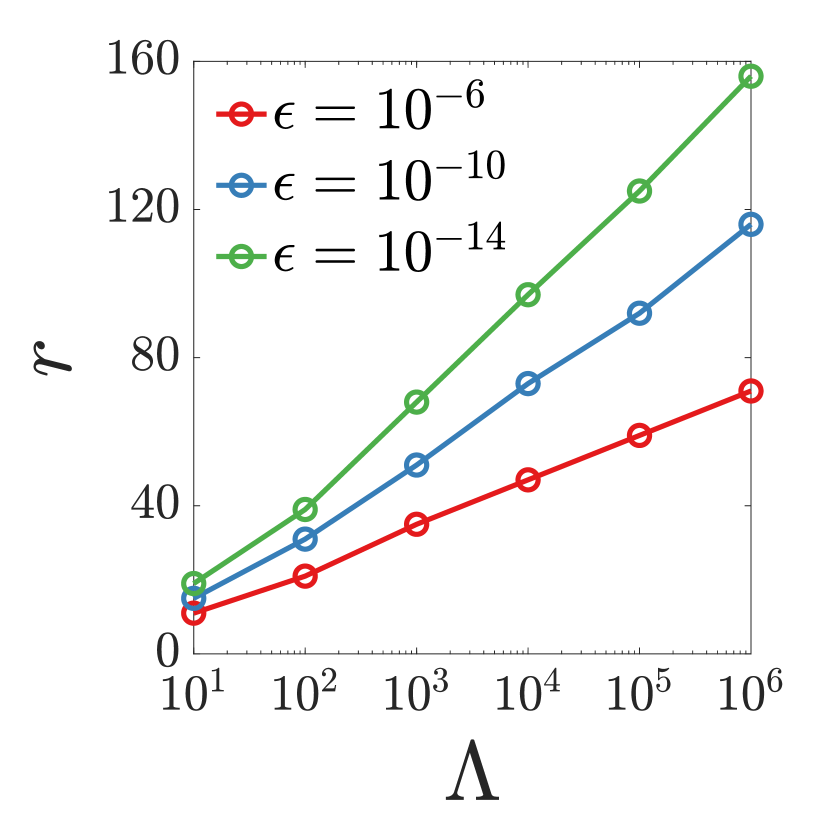
Figure 1: Number $r$ of DLR basis functions for different values of $\Lambda$ and $\epsilon$; observed scaling is $r=\mathcal{O}\left(\log\left(\Lambda\right)\log\left(1/\epsilon\right)\right)$. This figure uses data from [8].

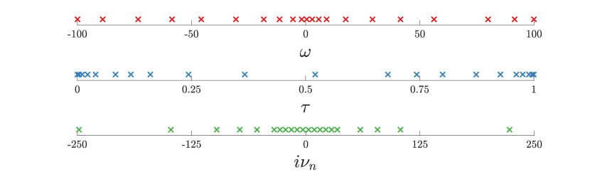
Figure 2: The 21 DLR frequencies, imaginary time nodes, and Matsubara frequency nodes for $\Lambda=100$ and $\epsilon=10^{-6}$. The clustering of each set of nodes reflects the structure of Green’s functions in the respective domains, and is automatically determined by the pivoted QR procedure.

The DLR coefficients $\widehat{g}_{l}$ of a given Green’s function $G$ can be recovered directly from samples $\{G(\tau_{k}^{s})\}_{k=1}^{n}$, for some sampling nodes $\tau_{k}^{s}$. This can be done by solving a linear system

$$\sum_{l=1}^{r}K(\tau_{k}^{s},\omega_{l})\widehat{g}_{l}=G(\tau_{k}^{s}),$$ (6)

for $k=1,\ldots,n$. We consider two possible scenarios: (i) Applying the rank revealing row pivoted QR algorithm to the matrix $K(\tau_{i}^{f},\omega_{l})$ yields a set of interpolation nodes $\{\tau_{k}\}_{k=1}^{r}$, called the DLR imaginary time nodes, such that the coefficients can be recovered from the samples $\{G(\tau_{k})\}_{k=1}^{r}$. Thus, if $G(\tau)$ can be evaluated at arbitrary imaginary time points, then we can take $n=r$ and $\tau_{k}^{s}=\tau_{k}$ in (6) and solve the resulting small square linear system to obtain an interpolant of $G(\tau)$. An example of the DLR imaginary time nodes is shown in the second panel of Figure 2. (ii) If samples of $G$ are given at a collection of $n>r$ scattered or uniform grid points $\tau_{k}^{s}$, then (6) is an overdetermined system and can be solved by ordinary least squares fitting.

Since the DLR basis functions are given explicitly, a DLR expansion can be analytically transformed to the Matsubara frequency domain. We have

$$K(i\nu_{n},\omega)=\int_{0}^{\beta}K(\tau,\omega)e^{-i\nu_{n}\tau}\,d\tau=\left(\omega+i\nu_{n}\right)^{-1},$$ (7)

with the Matsubara frequencies given by

$$i\nu_{n}=\begin{cases}i(2n+1)\pi/\beta&\text{ for fermionic Green's functions}\\ i(2n)\pi/\beta&\text{ for bosonic Green's functions}\end{cases}$$ (8)

in unscaled coordinates. In scaled coordinates, we simply set $i\nu_{n}\leftarrow i\beta\nu_{n}$. The DLR expansion in the Matsubara frequency domain is then

$$G_{\text{DLR}}(i\nu_{n})=\sum_{l=1}^{r}K(i\nu_{n},\omega_{l})\widehat{g}_{l}.$$

As in the imaginary time domain, there is a set of Matsubara frequencies $\{i\nu_{n_{k}}\}_{k=1}^{r}$, the DLR Matsubara frequency nodes, such that the coefficients can be recovered from samples $\{G(i\nu_{n_{k}})\}_{k=1}^{r}$ by interpolation; or, one can recover the expansion by least squares fitting. An example of the DLR Matsubara frequency nodes for a given choice of $\Lambda$ and $\epsilon$ is shown in the third panel of Figure 2.

For further details on the algorithm used to obtain the DLR frequencies, imaginary time nodes, and Matsubara frequencies, as well as a detailed analysis of the accuracy and stability of the method, we again refer the reader to [8].

3 Features and layout of the library

We list the main capabilities of libdlr:

• Given a choice of $\Lambda$ and $\epsilon$, obtain the DLR frequencies $\{\omega_{l}\}_{l=1}^{r}$ characterizing the DLR basis

• Obtain the DLR imaginary time and Matsubara frequency grids

• Recover the DLR coefficients of an imaginary time Green’s function from its samples on the DLR grids or from noisy data

• Evaluate a DLR expansion at arbitrary points in the imaginary time and Matsubara frequency domains

• Compute the convolution of imaginary time Green’s functions

• Solve the Dyson equation in imaginary time or Matsubara frequency

The computational cost of building the DLR basis and grids is typically negligible even for large values of $\Lambda$, and subsequent operations involve standard numerical linear algebra procedures with small matrices.

libdlr is implemented in Fortran, provides a C header interface, and includes a Python module, pydlr. More information on pydlr is contained in Appendix A. The documentation for the library [12] includes installation intructions, API information, and several examples. The source code is available as a Git repository [13]. The subfolder libdlr/test contains example programs which are run after compilation as tests, and the subfolder libdlr/demo contains additional example programs. An example C program using the C header interface may be found in libdlr/test/ha_it.c.

We have made the Julia package Lehmann.jl, which implements functionality similar to libdlr, available in a separate Git repository [14]. More information on Lehmann.jl is contained in Appendix B, and in the documentation [15].

4 Examples of usage

We describe two examples illustrating the functionality of libdlr. First, we demonstrate recovery of the DLR coefficients of a Green’s function both from its values on the DLR imaginary time grid and from noisy data on a uniform grid. Second, we demonstrate the process of solving the Dyson equation self-consistently for the Sachdev-Ye-Kitaev model [16, 17, 18]. All examples are implemented in Fortran; Appendices A and B contain analogous examples implemented using pydlr and Lehmann.jl, respectively.

4.1 Obtaining a DLR expansion from Green’s function samples

We consider the Green’s function given by the Lehmann representation (1) with spectral density

$$\rho(\omega)=\frac{2}{\pi}\sqrt{1-\omega^{2}}\,\theta(1-\omega^{2}).$$ (9)

Here, $\theta$ is the Heaviside function. In practical calculations, the spectral density is usually not known, so one must recover the DLR from samples of the Green’s function itself. We use a Green’s function with known spectral density for illustrative purposes, since we can evaluate it with high accuracy by numerical integration of (1) and thereby test our results.

Since $\operatorname{supp}\rho\subset[-1,1]$, we can take the frequency support cutoff $\omega_{\max}=1$. Then $\Lambda=\beta\omega_{\max}\geq\beta$ is a sufficient high energy cutoff. In practice, $\omega_{\max}$ can typically be estimated on physical grounds, giving an estimate of $\Lambda$. Calculations can then be converged with respect to $\Lambda$ to ensure accuracy. The error tolerance $\epsilon$ should be chosen based on the desired accuracy, in order to obtain the smallest possible number of basis functions. In this example, we take $\beta=1000$, and fix $\Lambda=1000$.

We note also that libdlr routines work by default with matrix-valued Green’s functions $G_{ij}$, where $i$ and $j$ are typically orbital indices. However, in all examples presented here, we work with scalar-valued Green’s functions, and therefore set the parameter n determining the number of orbital indices to $1$.

4.1.1 Recovery of DLR from imaginary time grid values

We first consider recovery of the DLR coefficients $\widehat{g}_{l}$ from samples of $G(\tau)$ on the DLR imaginary time nodes $\tau_{k}$. This is the first scenario mentioned in Section 2, and generates an interpolant at the nodes $\tau_{k}$. Figure 3 shows a condensed version of a Fortran code implementing the example using libdlr. In this and all other sample Fortran codes, we do not show variable allocations or steps which do not involve libdlr subroutines, as indicated in the code comments. A complete Fortran code demonstrating this example can be found in the file libdlr/demo/sc_it.f90. The file libdlr/demo/sc_mf.f90 contains a demonstration of the process of obtaining a DLR from values of a Green’s function on the DLR Matsubara frequency nodes.

⬇

! Set parameters and build DLR basis, imaginary time grid

lambda = 1000.0d0 ! DLR high energy cutoff

eps = 1.0d-10 ! DLR error tolerance

xi = -1 ! Fermionic Green’s function

n = 1 ! # orbital indices

call dlr_it_build(lambda,eps,r,dlrrf,dlrit)

! Recovery of DLR from DLR imaginary time nodes (assume values of G

! on DLR imaginary time grid dlrit stored in array g)

call dlr_it2cf_init(r,dlrrf,dlrit,it2cf,it2cfp)

call dlr_it2cf(r,n,it2cf,it2cfp,g,gc)

! Evaluate on imaginary time output grid of nout points

call eqpts_rel(nout,tout) ! Equispaced grid in relative format

do i=1,nout

call dlr_it_eval(r,n,dlrrf,gc,tout(i),gout_it(i))

enddo

! Evaluate on Matsubara frequency output grid with cutoff index

! nmfmax

do nmf=-nmfmax,nmfmax

call dlr_mf_eval(r,n,dlrrf,xi,gc,nmf,gout_mf(nmf))

enddo

Figure 3: libdlr Fortran code to obtain DLR from values of a Green’s function on the DLR imaginary time grid. To emphasize the usage of libdlr subroutines, we do not show variable allocations or the external procedures used to sample the Green’s function, as indicated in the code comments.

We first set $\Lambda$ and $\epsilon$, and then build the DLR basis by obtaining the DLR real frequencies $\omega_{l}$, stored in the array dlrrf, using the subroutine dlr_it_build. This subroutine also produces the $r$ DLR imaginary time nodes $\tau_{k}$, which are stored in the array dlrit.

Next, we assume that the values $G(\tau_{k})$ have been obtained by some external procedure, and stored in the array g. In this case, we used numerical integration with the known spectral function to obtain the samples. To obtain the DLR coefficients $\widehat{g}_{l}$, one must solve the linear system (6), with $n=r$. The subroutine dlr_it2cf_init initializes this procedure by computing the LU factorization of the system matrix. The LU factors and pivots are stored in the arrays it2cf and it2cfp, respectively. The linear solve is then carried out by the subroutine dlr_it2cf, which returns the DLR coefficients $\widehat{g}_{l}$ in the array gc.

We can then evaluate the DLR expansion on output grids in imaginary time and Matsubara frequency. The subroutine eqpts_rel generates a uniform grid of imaginary time points in the relative format employed by the library (see Appendix C for an explanation of the relative format) and dlr_it_eval evaluates the expansion. The subroutine dlr_mf_eval evaluates the DLR expansion in the Matsubara frequency domain.

4.1.2 Recovery of DLR from noisy data

We next consider DLR fitting from noisy data, the second scenario mentioned in Section 2. A condensed sample code is given in Figure 4, and a complete example can be found in the file libdlr/demo/sc_it_fit.f90. We assume noisy samples $G(\tau_{k}^{s})$ have been obtained by an external procedure and stored in the array g. The subroutine dlr_it_fit fits a DLR expansion to the data by solving the overdetermined system (6). The resulting DLR coefficients, stored in the array gc, can be used to evaluate the DLR expansion as in the previous example.

⬇

! Set parameters and build DLR basis, imaginary time grid

lambda = 1000.0d0 ! DLR high energy cutoff

eps = 1.0d-4 ! DLR error tolerance

n = 1 ! # orbital indices

call dlr_it_build(lambda,eps,r,dlrrf,dlrit)

! Recovery of DLR from noisy data on uniform grid (assume data

! given at m equispaced grid points t stored in array g)

call dlr_it_fit(r,n,dlrrf,m,t,g,gc)

Figure 4: libdlr Fortran code to obtain DLR from noisy data on a uniform grid.

4.1.3 Numerical results

Figure 5 presents some numerical results for the two examples. In Figure 5a, we plot the Green’s function $G(\tau)$ with spectral density (9) and $\beta=1000$, along with noisy data obtained on a uniform grid of $n=2500$ points by adding uniform random numbers of magnitude $\eta=10^{-2}$ to accurate values computed by numerical integration. We see that the DLR fit $G_{\text{DLR}}$ to this data with $\epsilon=10^{-2}$ agrees well with $G(\tau)$. Pointwise errors for this example, and examples with different noise levels $\eta$, are given in Figure 5c. In all cases we take $\epsilon=\eta$, and observe that the DLR fitting process is stable; the fitting process does not introduce a significant error above the magnitude of the noise. Pointwise errors for the DLR obtained from numerically exact samples on the DLR imaginary time grid are shown in Figure 5b, and we see that the error is well controlled by $\epsilon$.

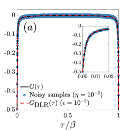
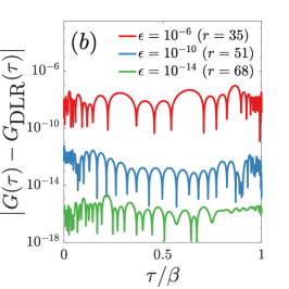
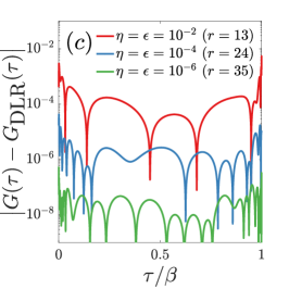
Figure 5: DLR expansion of a Green’s function with spectral density (9), for $\beta=1000$, $\Lambda=1000$. (a) Noisy imaginary time data (noise of magnitude $\eta=10^{-2}$) with DLR fit ($\epsilon=10^{-2}$, $r=13$). (b) Error of DLR expansion obtained from imaginary time grid sampling, with different choices of $\epsilon$. DLR rank $r$ obtained for each choice of $\epsilon$ also indicated. (c) Error of DLR expansion obtained from fit of $n=2500$ noisy uniform grid samples, with different noise levels $\eta$, and $\epsilon=\eta$.

4.2 Solving the Sachdev-Ye-Kitaev model

The Dyson equation for a given self-energy $\Sigma$ can be written in the Matsubara frequency domain as

$$G^{-1}(i\nu_{n})=G^{-1}_{0}(i\nu_{n})-\Sigma(i\nu_{n}).$$ (10)

Here $G_{0}(i\nu_{n})=(i\nu_{n}+\mu)^{-1}$ is the free particle Green’s function, with chemical potential $\mu$. This equation can be solved for $G$ by pointwise inversion on the $r$ DLR Matsubara frequency nodes.

In typical applications, $\Sigma$ is a function of $G$, $\Sigma=\Sigma\left[G\right]$, which is most easily evaluated in the imaginary time domain. In this case, (10) becomes nonlinear, and must be solved by self-consistent iteration. The standard method is to solve the Dyson equation using (10) for a given iterate of $\Sigma$, transform the solution $G$ to the imaginary time domain to evaluate a new iterate of $\Sigma$, and then transform $\Sigma$ back to the Matsubara frequency domain to solve (10) for the next iteration. The standard implementation of this approach represents $G$ and $\Sigma$ on fine equispaced grids in imaginary time, and uses the fast Fourier transform to move between the imaginary time and Matsubara frequency domains. The process can be carried out significantly more efficiently using the DLR.

As an example, we consider the Dyson equation given by (10) with the Sachdev-Ye-Kitaev (SYK) [16, 17, 18] self-energy

$$\Sigma(\tau)=J^{2}G^{2}(\tau)G(\beta-\tau).$$ (11)

Here $J$ is a coupling constant. We consider this example with $\beta=1000$, $\mu=0$, and $J=1$, and set $\Lambda=5000$. We note that $G$ is a fermionic Green’s function, so we use a fermionic Matsubara frequency grid.

Figure 6 gives sample code for a solver which uses a weighted fixed point iteration to handle the nonlinearity:

$$\Sigma^{(m+1)}=\Sigma[w\,G^{(m)}+(1-w)\,G^{(m-1)}].$$ (12)

Here, $m$ refers to the iterate, and $w$ is a weighting parameter which can be selected to improve convergence; we use $w=0.3$. A complete code demonstrating this example can be found in the file libdlr/demo/syk_mf.f90.

⬇

! Set DLR parameters and build DLR basis, imaginary time grid,

! Matsubara frequency grid

lambda = 5000.0d0 ! DLR high energy cutoff

eps = 1.0d-10 ! DLR error tolerance

nmfmax = 5000 ! DLR Matsubara frequency cutoff

xi = -1 ! Fermionic Green’s function

n = 1 ! # orbital indices

call dlr_it_build(lambda,eps,r,dlrrf,dlrit)

call dlr_mf(nmfmax,r,dlrrf,xi,dlrmf)

! Set problem parameters and parameters for nonlinear iteration

beta = 1000.0d0 ! Inverse temperature

mu = 0.0d0 ! Chemical potential

j = 1.0d0 ! Coupling constant

numit = 100 ! Max # weighted fixed point iterations

fptol = 1.0d-10 ! Fixed point tolerance

w = 0.3d0 ! Fixed point weighting parameter

! Initialize transformations between imaginary time, Matsubara

! frequency grids and DLR coefficients

call dlr_it2cf_init(r,dlrrf,dlrit,it2cf,it2cfp)

call dlr_cf2it_init(r,dlrrf,dlrit,cf2it)

call dlr_mf2cf_init(nmfmax,r,dlrrf,dlrmf,xi,mf2cf,mf2cfp)

call dlr_cf2mf_init(r,dlrrf,dlrmf,xi,cf2mf)

call dlr_it2itr_init(r,dlrrf,dlrit,it2cf,it2cfp,it2itr)

! Get free particle Green’s function on Matsubara frequency grid

call g0_mf(beta,r,dlrmf,mu,g0)

! Get free particle Green’s function on imaginary time grid for

! initial guess in nonlinear iteration

call g0_it(beta,r,dlrit,mu,g)

! Weighted fixed point iteration

do i=1,numit

gprev = g ! Store previous iterate

call sigfun(r,j,it2itr,g,sig) ! Evaluate self-energy

call dlr_it2cf(r,n,it2cf,it2cfp,sig,sigc) ! Imaginary time grid -> DLR coeffs

call dlr_cf2mf(r,n,cf2mf,sigc,sigmf) ! DLR coeffs -> Matsubara frequency grid

call dyson_mf(beta,r,n,g0,sigmf,gmf) ! Solve Dyson equation

call dlr_mf2cf(r,n,mf2cf,mf2cfp,gmf,gc) ! Matsubara frequency grid -> DLR coeffs

call dlr_cf2it(r,n,cf2it,gc,g) ! DLR coeffs -> imaginary time grid

if (maxval(abs(gprev-g))<fptol) then ! Check self-consistency

return

else

g = w*g + (1.0d0-w)*gprev ! Reweight

endif

enddo

Figure 6: libdlr Fortran code to solve the SYK model.

As in the previous example, the code begins by obtaining the DLR frequencies and imaginary time grid. Here, the DLR Matsubara frequency grid is also built, using the subroutine dlr_mf, with a Matsubara frequency cutoff nmax. This cutoff should in principle be taken larger and larger until the selected DLR Matsubara frequencies no longer change, but in practice we find that setting it to $\Lambda$ is usually sufficient (see the discussion in [8, Sec. IV D]).

The next several lines define physical problem parameters, and parameters for the weighted fixed point iteration. Then, several initialization routines are called which prepare transformations between the imaginary time and Matsubara frequency grid representations of the Green’s function, and the DLR coefficients. These transformations are used to convert between imaginary time and Matsubara frequency representations in the self-consistent iteration. The subroutine dlr_it2itr_init prepares a transformation between a Green’s function $G(\tau)$ on the imaginary time grid and its reflection $G(\beta-\tau)$ on the same grid, which is needed to evaluate the SYK self-energy.

The free particle Green’s function $G_{0}$ appearing in (10) is then evaluated on the Matsubara frequency grid, since it appears in the Dyson equation, and on the imaginary time grid, to serve as an initial guess in the iteration. In the weighted fixed point iteration, the self-energy is evaluated on the imaginary time grid, and then transformed to the Matsubara frequency domain, where the Dyson equation is solved. Then the result is transformed back to the imaginary time grid, where the self-consistency of the solver is checked. Figure 7 shows the subroutine used to evaluate the SYK self-energy in imaginary time. Once self-consistency is reached, the solution is returned on the imaginary time grid. It can be expanded in a DLR and evaluated in imaginary time or Matsubara frequency as in the previous example.

⬇

subroutine sigfun(r,j,it2itr,g,sig)

! Evaluate SYK self-energy

n = 1 ! Scalar-valued G

call dlr_it2itr(r,n,it2itr,g,gr) ! Get G(beta-tau)

sig = j*j*g*g*gr ! Get Sigma(tau)

end subroutine sigfun

Figure 7: Evaluation subroutine for SYK self-energy, used in the SYK solver shown in Figure 6.

Plots of the solution and of the DLR nodes are given in Figure 8, both in imaginary time and Matsubara frequency. For $\Lambda=5000$ and $\epsilon=10^{-10}$, there are $r=66$ DLR nodes discretizing each domain.

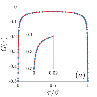
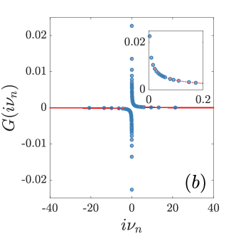
Figure 8: Solution of the SYK model with $\beta=1000$, $\mu=0$, and $J=1$. (a) $G(\tau)$, with $r=66$ DLR imaginary time nodes for $\epsilon=10^{-10}$ accuracy indicated by the blue circles. (b) $G(i\nu_{n})$, with DLR Matsubara frequency nodes.

We remark that the Dyson equation (10) may be written in the imaginary time domain as

$$G(\tau)-\int_{0}^{\beta}d\tau^{\prime}G_{0}(\tau-\tau^{\prime})\int_{0}^{\beta}d\tau^{\prime\prime}\Sigma(\tau^{\prime}-\tau^{\prime\prime})G(\tau^{\prime\prime})=G_{0}(\tau).$$ (13)

In [8], an efficient method is presented of solving (13) by discretizing the convolutions using the DLR. This approach may be advantageous in certain cases, and can also be implemented using libdlr. A demonstration for the SYK model is given in the file libdlr/demo/syk_it.f90.

We also note that the convergence properties of nonlinear iteration in the self-consistent solution of the Dyson equation are problem-dependent. For the SYK model (11), which belongs to a particular subclass of approximations [19], we find that the weighted fix point iteration (12) may fail to converge or converge to spurious local fixed points, particularly at extremely low temperatures. Many standard strategies can be used to improve convergence, including the careful selection of an initial guess by adiabatic variation of parameters like $\beta$ or $\mu$, mixing, and more sophisticated nonlinear iteration procedures. Two other methods have been observed to improve performance in certain difficult cases: the use of explicitly symmetrized DLR grids, and mild oversampling in the Matsubara frequency domain followed by least squares fitting to a DLR expansion. These are topics of our current research, and will be reported on in detail at a later date. Lastly, we have observed that solving (13) directly in the imaginary time domain, as mentioned in the previous paragraph, tends to lead to more robust convergence.

5 Conclusion

libdlr facilitates the efficient representation and manipulation of imaginary time Green’s functions using the DLR. In this framework, working with imaginary time Green’s functions is as simple as with standard discretizations, but involves many fewer degrees of freedom, and user-tuneable accuracy down to the level of machine precision.

As a result, we anticipate the use of the DLR as a basic working tool a variety of equilibrium applications, including continous-time quantum Monte Carlo [20], dynamical mean-field theory [21], self-consistent perturbation theory in both quantum chemistry (GF2) [22, 23, 24, 25] and condensed matter physics [26], as well as Hedin’s GW approximation [27, 28], including vertex corrections [29, 30]. In [31], the DLR was used to discretize imaginary time variables in equilibrium real time contour Green’s functions. In nonequilibrium calculations involving two-time Green’s functions, it can replace the equispaced imaginary time grids currently in use [32, 33], and further improve the efficiency of algorithms making use of low rank compression to reduce the cost of time propagation [34].

Appendix A Python module pydlr

The library libdlr provides a stand-alone Python module pydlr, so that small-scale tests can be easily carried out in Python. The libdlr documentation [12] includes usage examples and API instructions for pydlr. Here, we show how the examples discussed in Section 4 can be implemented using pydlr.

1. The first example, demonstrating recovery of the DLR coefficients $\widehat{g}_{l}$ from values of a Green’s function at the DLR imaginary time nodes $\tau_{k}$, is shown in Figure 9. We also demonstrate the evaluation of the DLR at arbitrary imaginary time points. We again use the example of the Green’s function with spectral density (9).

2. The second example, demonstrating recovery of the DLR coefficients from noisy data in imaginary time, is shown in Figure 10.

3. The final example, demonstrating the iterative solution of the SYK model, is shown in Figure 11.

⬇

import numpy as np

from pydlr import dlr

from pydlr.utils import analytic_bethe_G_tau as true_G_tau

beta = 1000. # Inverse temperature

d = dlr(lamb=1000., eps=1e-14) # Initialize DLR object

tau_k = d.get_tau(beta) # DLR imaginary time points

G_k = true_G_tau(tau_k, beta) # Evaluate known G at tau_k

G_x = d.dlr_from_tau(G_k) # DLR coeffs from G_k

tau_i = np.linspace(0, beta, num=40) # Equispaced tau grid

G_i = d.eval_dlr_tau(G_x, tau_i, beta) # Evaluate DLR at tau_i

Figure 9: pydlr Python code to obtain DLR from values of the Green’s function with spectral density (9) on the DLR imaginary time grid, and to evaluate the DLR at arbitrary points in imaginary time.

⬇

import numpy as np

from pydlr import dlr

eta = 1e-3 # Noise level

beta = 1000 # Inverse temperature

d = dlr(lamb=1000., eps=1e-14) # Initialize DLR object

# Generate noisy data

from pydlr.utils import analytic_bethe_G_tau as true_G_tau

tau_i = np.linspace(0, beta, num=100)

G_i = true_G_tau(tau_i, beta)

G_i_noisy = G_i + eta*(np.random.random(G_i.shape)-.5)

# Fit DLR coeffs from noisy data

G_x = d.lstsq_dlr_from_tau(tau_i, G_i_noisy, beta)

# Evaluate DLR

G_i_fit = d.eval_dlr_tau(G_x, tau_i, beta)

Figure 10: pydlr Python code to obtain DLR from noisy data on a uniform grid.

⬇

import numpy as np

from pydlr import dlr

def syk_sigma_dlr(d, G_x, beta, J=1.):

tau_k = d.get_tau(beta) # DLR imaginary time nodes

tau_k_rev = beta - tau_k # Reversed imaginary time nodes

G_k = d.tau_from_dlr(G_x) # G at tau_k

G_k_rev = d.eval_dlr_tau(G_x, tau_k_rev, beta) # G at beta - tau_k

Sigma_k = J**2 * G_k**2 * G_k_rev # SYK self-energy in imaginary time

Sigma_x = d.dlr_from_tau(Sigma_k) # DLR coeffs of self-energy

return Sigma_x

def solve_syk_with_fixpoint_iter(d, mu, beta, tol=1e-14, mix=0.3, maxiter=100):

Sigma_q = np.zeros((len(d), 1, 1)) # Initial guess

for iter in range(maxiter):

G_q = d.dyson_matsubara(np.array([[-mu]]), Sigma_q, beta) # Solve Dyson

G_x = d.dlr_from_matsubara(G_q, beta) # Get DLR coeffs

Sigma_x_new = syk_sigma_dlr(d, G_x, beta) # Compute self-energy

Sigma_q_new = d.matsubara_from_dlr(Sigma_x_new, beta) # Transform self-energy to Matsubara frequency

if np.max(np.abs(Sigma_q_new - Sigma_q)) < tol: break # Check self-consistency

Sigma_q = mix * Sigma_q_new + (1-mix) * Sigma_q # Linear mixing

return G_q

d = dlr(lamb=5000., eps=1e-14)

G_q = solve_syk_with_fixpoint_iter(d, mu=0., beta=1000.)

Figure 11: pydlr Python code to solve the SYK model.

Appendix B Julia module Lehmann.jl

The stand-alone package Lehmann.jl provides a pure Julia implementation of the DLR. The Lehmann.jl documentation [15] includes usage examples and API instructions. The examples discussed in Section 4 and Appendix A can be implemented using Lehmann.jl, as shown in Figures 12, 13, and 14.

⬇

using Lehmann

beta = 1000.0 # Inverse temperature

Euv = 1.0 # We define Lambda = Euv * beta

d = DLRGrid(Euv, beta, rtol = 1e-14, isFermi = true) # Initialize DLR object (fermionic Green’s function)

tau_k = d.tau # DLR imaginary time points

G_k = true_G_tau(tau_i, d.beta) # Evaluate known G at tau_k

G_x = tau2dlr(d, G_k) # DLR coeffs from G_k

tau_i = collect(LinRange(0, d.beta, 40)) # Equispaced tau grid

G_i = dlr2tau(d, G_x, tau_i) # Evaluate DLR at tau_i

Figure 12: Lehmann.jl Julia code to obtain DLR from values of the Green’s function with spectral density (9) on the DLR imaginary time grid, and to evaluate the DLR at arbitrary points in imaginary time.

⬇

using Lehmann

eta = 1e-3 # Noise level

beta = 1000 # Inverse temperature

Euv = 1.0 # Lambda = Euv * beta

d = DLRGrid(Euv, beta, rtol = 1e-14, isFermi = true) # Initialize DLR object

# Generate noisy data

tau_i = collect(LinRange(0, d.beta, 100))

G_i = true_G_tau(tau_i, d.beta)

G_i_noisy = G_i .+ eta .* (rand(length(G_i)) .- 0.5)

# Fit DLR coeffs from noisy data

G_x = tau2dlr(d, G_i_noisy, tau_i)

# Evaluate DLR

G_i_fit = dlr2tau(d, G_x, tau_i)

Figure 13: Lehmann.jl Julia code to obtain DLR from noisy data on a uniform grid.

⬇

using Lehmann

function syk_sigma_dlr(d, G_x, J = 1.0)

tau_k = d.tau # DLR imaginary time nodes

tau_k_rev = d.beta .- tau_k # Reversed imaginary time nodes

G_k = dlr2tau(d, G_x) # G at tau_k

G_k_rev = dlr2tau(d, G_x, tau_k_rev) # G at beta - tau_k

Sigma_k = J .^ 2 .* G_k .^ 2 .* G_k_rev # SYK self-energy in imaginary time

Sigma_x = tau2dlr(d, Sigma_k) # DLR coeffs of self-energy

return Sigma_x

end

function solve_syk_with_fixpoint_iter(d, mu, tol = d.rtol, mix = 0.3, maxiter = 100)

Sigma_q = zeros(length(d)) # Initial guess

G_q = zeros(ComplexF64, length(d))

for iter in 1:maxiter

G_q .= -1 ./ (d.omegaN * 1im .- mu .+ Sigma_q) # Solve Dyson

G_x = matfreq2dlr(d, G_q) # Get DLR coeffs

Sigma_x_new = syk_sigma_dlr(d, G_x) # Compute self-energy

Sigma_q_new = dlr2matfreq(d, Sigma_x_new) # Transform self-energy to Matsubara frequency

if maximum(abs.(Sigma_q_new .- Sigma_q)) < tol # Check self-consistency

break

end

Sigma_q = mix * Sigma_q_new + (1 - mix) * Sigma_q # Linear mixing

end

return G_q

end

d = DLRGrid(Euv = 5.0, beta = 1000.0, isFermi = true, rtol = 1e-14)

G_q = solve_syk_with_fixpoint_iter(d, 0.0)

Figure 14: Lehmann.jl Julia code to solve the SYK model.

Appendix C Stable kernel evaluation and relative format for imaginary time points

In libdlr, we work in the dimensionless variables defined at the beginning of Section 2, in which the kernel $K(\tau,\omega)$ is given by

$$K(\tau,\omega)=\frac{e^{-\tau\omega}}{1+e^{-\omega}}$$ (14)

for $\tau\in[0,1]$ and $\omega\in(-\infty,\infty)$. When $\omega\geq 0$, this formula is numerically stable. If $\omega\ll 0$, it can overflow, and we instead use the mathematically equivalent formula

$$K(\tau,\omega)=\frac{e^{(1-\tau)\omega}}{1+e^{\omega}}.$$ (15)

This formula, however, leads to another problem: when $\left|\omega\right|$ is large, catastrophic cancellation in the calculation of $1-\tau$ for $\tau$ near $1$ leads to a loss of accuracy in floating point arithmetic.

To fix this problem, we define a relative format for representing imaginary time values $\tau\in(0.5,1)$. Rather than representing them directly, which we refer to as the absolute format, we instead store $\tau^{*}=\tau-1\in(-0.5,0)$ to full relative accuracy. Then the kernel is evaluated as $K(-\tau^{*},-\omega)$. If $\omega>0$, (15) then yields the numerically stable formula

$$K(-\tau^{*},-\omega)=\frac{e^{-(1+\tau^{*})\omega}}{1+e^{-\omega}}.$$

Since

$$\frac{e^{-(1+\tau^{*})\omega}}{1+e^{-\omega}}=\frac{e^{-\tau\omega}}{1+e^{-\omega}}=K(\tau,\omega),$$

this formula gives the desired result. If $\omega<0$, then (14) yields

$$K(-\tau^{*},-\omega)=\frac{e^{-\tau^{*}\omega}}{1+e^{\omega}}$$ (16)

which is also numerically stable. We again have

$$\frac{e^{-\tau^{*}\omega}}{1+e^{\omega}}=\frac{e^{(1-\tau)\omega}}{1+e^{\omega}}=K(\tau,\omega).$$

Let us illustrate the advantage with a concrete example. For simplicity, we assume we are working in three-digit arithmetic. We first consider the evaluation of $K(\tau,\omega)$ for $\tau=$0.50110-3$$ and $\omega=1000$. No problem arises in this case; we use the formula (14), and obtain the correct value

$$K(\tau,\omega)=\frac{e^{-0.501}}{1+e^{-1000}}.$$

However, if we instead want to calculate $K(\tau,\omega)$ for $\tau=1-$0.50110-3$=0.999499$ and $\omega=-1000$, the situation is different. In three-digit arithmetic, using the absolute format, we must round to $\tau=0.999$. Then we find

$$1-\tau=0.001\implies(1-\tau)\omega=-1,$$

and using (15) directly gives

$$K(\tau,\omega)=\frac{e^{-1}}{1+e^{-1000}},$$

which is far from the correct value. If we instead use the relative format, $\tau$ is stored as $\tau^{*}=$-0.50110-3$$, and using (16) gives precisely the correct value.

In practice, with double precision arithmetic, using the absolute format only leads to a significant loss of accuracy for very large $\Lambda$ and small $\epsilon$. However, to enable calculations to high accuracy in extreme scenarios, all subroutines in libdlr take in imaginary time values in the relative format. Of course, maintaining full relative precision also requires external procedures, such as those used to evaluate Green’s functions, to be similarly careful about this issue.

Many users are likely not operating in regimes in which it is important to maintain full relative precision for extreme parameter values. These users can simply ignore this discussion. However, they must still convert imaginary time values to the relative format before using them as inputs to libdlr subroutines (though, of course, imaginary time values which are converted from the absolute format to the relative format are only accurate to the original absolute precision). The subroutine abs2rel performs this conversion. Similarly, the subroutine rel2abs converts imaginary time values in the relative format used by libdlr to the ordinary absolute format.

References

- [1] L. Boehnke, H. Hafermann, M. Ferrero, F. Lechermann, and O. Parcollet, “Orthogonal polynomial representation of imaginary-time Green’s functions,” Phys. Rev. B, vol. 84, p. 075145, 2011.
- [2] E. Gull, S. Iskakov, I. Krivenko, A. A. Rusakov, and D. Zgid, “Chebyshev polynomial representation of imaginary-time response functions,” Phys. Rev. B, vol. 98, p. 075127, 2018.
- [3] X. Dong, D. Zgid, E. Gull, and H. U. R. Strand, “Legendre-spectral Dyson equation solver with super-exponential convergence,” J. Chem. Phys., vol. 152, no. 13, p. 134107, 2020.
- [4] H. Shinaoka, J. Otsuki, M. Ohzeki, and K. Yoshimi, “Compressing Green’s function using intermediate representation between imaginary-time and real-frequency domains,” Phys. Rev. B, vol. 96, no. 3, p. 035147, 2017.
- [5] N. Chikano, J. Otsuki, and H. Shinaoka, “Performance analysis of a physically constructed orthogonal representation of imaginary-time Green’s function,” Phys. Rev. B, vol. 98, no. 3, p. 035104, 2018.
- [6] N. Chikano, K. Yoshimi, J. Otsuki, and H. Shinaoka, “irbasis: Open-source database and software for intermediate-representation basis functions of imaginary-time Green’s function,” Comput. Phys. Commun., vol. 240, pp. 181–188, 2019.
- [7] J. Li, M. Wallerberger, N. Chikano, C.-N. Yeh, E. Gull, and H. Shinaoka, “Sparse sampling approach to efficient ab initio calculations at finite temperature,” Phys. Rev. B, vol. 101, no. 3, p. 035144, 2020.
- [8] J. Kaye, K. Chen, and O. Parcollet, “Discrete Lehmann representation of imaginary time Green’s functions,” Phys. Rev. B, vol. 105, p. 235115, 2022.
- [9] M. Jarrell and J. Gubernatis, “Bayesian inference and the analytic continuation of imaginary-time quantum Monte Carlo data,” Phys. Rep., vol. 269, no. 3, pp. 133–195, 1996.
- [10] H. Cheng, Z. Gimbutas, P.-G. Martinsson, and V. Rokhlin, “On the compression of low rank matrices,” SIAM J. Sci. Comput., vol. 26, no. 4, pp. 1389–1404, 2005.
- [11] E. Liberty, F. Woolfe, P.-G. Martinsson, V. Rokhlin, and M. Tygert, “Randomized algorithms for the low-rank approximation of matrices,” Proc. Natl. Acad. Sci. U.S.A., vol. 104, no. 51, pp. 20167–20172, 2007.
- [12] https://libdlr.readthedocs.io.
- [13] https://github.com/jasonkaye/libdlr.
- [14] https://github.com/numericalEFT/lehmann.jl.
- [15] https://numericaleft.github.io/Lehmann.jl/dev/.
- [16] S. Sachdev and J. Ye, “Gapless spin-fluid ground state in a random quantum Heisenberg magnet,” Phys. Rev. Lett., vol. 70, pp. 3339–3342, 1993.
- [17] Y. Gu, A. Kitaev, S. Sachdev, and G. Tarnopolsky, “Notes on the complex Sachdev-Ye-Kitaev model,” J. High Energy Phys., vol. 2020, no. 2, pp. 1–74, 2020.
- [18] D. Chowdhury, A. Georges, O. Parcollet, and S. Sachdev, “Sachdev-Ye-Kitaev models and beyond: A window into non-Fermi liquids,” 2021. arXiv:2109.05037.
- [19] M. J. Hyrkäs, D. Karlsson, and R. van Leeuwen, “Cutting rules and positivity in finite temperature many-body theory,” 2022. arXiv:2203.11083.
- [20] E. Gull, A. J. Millis, A. I. Lichtenstein, A. N. Rubtsov, M. Troyer, and P. Werner, “Continuous-time Monte Carlo methods for quantum impurity models,” Rev. Mod. Phys., vol. 83, pp. 349–404, 2011.
- [21] A. Georges, G. Kotliar, W. Krauth, and M. J. Rozenberg, “Dynamical mean-field theory of strongly correlated fermion systems and the limit of infinite dimensions,” Rev. Mod. Phys., vol. 68, no. 1, pp. 13–125, 1996.
- [22] N. E. Dahlen and R. van Leeuwen, “Self-consistent solution of the Dyson equation for atoms and molecules within a conserving approximation,” J. Chem. Phys., vol. 122, no. 16, p. 164102, 2005.
- [23] J. J. Phillips and D. Zgid, “Communication: The description of strong correlation within self-consistent Green’s function second-order perturbation theory,” J. Chem. Phys., vol. 140, no. 24, p. 241101, 2014.
- [24] M. Schüler and Y. Pavlyukh, “Spectral properties from Matsubara Green’s function approach: Application to molecules,” Phys. Rev. B, vol. 97, p. 115164, 2018.
- [25] X. Dong, D. Zgid, E. Gull, and H. U. R. Strand, “Legendre-spectral Dyson equation solver with super-exponential convergence,” J. Chem. Phys., vol. 152, no. 13, p. 134107, 2020.
- [26] A. A. Rusakov and D. Zgid, “Self-consistent second-order Green’s function perturbation theory for periodic systems,” J. Chem. Phys., vol. 144, no. 5, 2016.
- [27] L. Hedin, “New method for calculating the one-particle Green’s function with application to the electron-gas problem,” Phys. Rev., vol. 139, no. 3A, 1965.
- [28] D. Golze, M. Dvorak, and P. Rinke, “The compendium: A practical guide to theoretical photoemission spectroscopy,” Front. Chem., vol. 7, p. 377, 2019.
- [29] A. L. Kutepov, “Electronic structure of and from a self-consistent vertex-corrected approach,” Phys. Rev. B, vol. 104, p. 085109, 2021.
- [30] G. Stefanucci, Y. Pavlyukh, A.-M. Uimonen, and R. van Leeuwen, “Diagrammatic expansion for positive spectral functions beyond : Application to vertex corrections in the electron gas,” Phys. Rev. B, vol. 90, p. 115134, 2014.
- [31] J. Kaye and H. U. R. Strand, “A fast time domain solver for the equilibrium Dyson equation,” 2021. arXiv:2110.06120.
- [32] A. Stan, N. E. Dahlen, and R. van Leeuwen, “Time propagation of the Kadanoff–Baym equations for inhomogeneous systems,” J. Chem. Phys., vol. 130, no. 22, p. 224101, 2009.
- [33] M. Schüler, D. Golež, Y. Murakami, N. Bittner, A. Herrmann, H. U. R. Strand, P. Werner, and M. Eckstein, “NESSi: The Non-Equilibrium Systems Simulation package,” Comput. Phys. Commun., vol. 257, p. 107484, 2020.
- [34] J. Kaye and D. Golež, “Low rank compression in the numerical solution of the nonequilibrium Dyson equation,” SciPost Phys., vol. 10, p. 91, 2021.