Uncertainty in Data-Driven Kalman Filtering for Partially known State-Space Models

Abstract

Providing a metric of uncertainty alongside a state estimate is often crucial when tracking a dynamical system. Classic state estimators, such as the kf (kf), provide a time-dependent uncertainty measure from knowledge of the underlying statistics; however, dl based tracking systems struggle to reliably characterize uncertainty. In this paper, we investigate the ability of kn, a recently proposed; hybrid; mb; deep state tracking algorithm, to estimate an uncertainty measure. By exploiting the interpretable nature of kn, we show that the error covariance matrix can be computed based on its internal features, as an uncertainty measure. We demonstrate that when the system dynamics are known, kn—which learns its mapping from data without access to the statistics—provides uncertainty similar to that provided by the kf; and while in the presence of evolution model-mismatch, kn provides a more accurate error estimation.

Index Terms—  kf, dl, uncertainty

1 Introduction

Tracking a hidden state vector from noisy observations in rt is at the core of many sp applications. A leading approach to the task is the kf [1], which operates with low complexity and achieves a mmse (mmse) in setups characterized by lg ss (ss) models. A key merit of the kf, which is of paramount importance in safety critical applications, e.g., autonomous driving, aviation, and medical, is its ability to provide uncertainty alongside state estimation [2, Ch. 4]. kf and its variants are mb (mb) algorithms, and are therefore sensitive to inaccuracies in modeling the system dynamics using the ss model.

The recent success of deep learning architectures, such as rnn [3] and attention mechanisms [4], in learning from complex time-series data in unstructured environments and in a model-agnostic manner, evoked interest in using them for tracking dynamical systems. However, the lack of interpretability of deep architectures and their inability to capture uncertainty [5], together with the fact that they require many trainable parameters and large data sets even for simple setups [6], limit their applicability for safety-critical applications in hardware-limited systems.

Characterizing uncertainty in dnn is an active area of research [7, 8, 9]. One approach is to use Bayesian dnn [10], which, when combined with ss models, enables extraction of the uncertainty. See, e.g., [11, 12, 13]. However, doing so relies on variational inference, which makes learning more complex and less scalable, and cannot be used directly for state estimation [5]. Alternatively, one can use deep learning techniques to estimate the ss model parameters and then plug them into a variant of a kf that provides uncertainty; e.g., [14, 15, 16, 17]. These approaches are limited in accuracy and complexity, requiring linearization of the second-order moments to compute the error covariance as required by the mb kf. The kf-inspired rnn proposed [5] was trained to predict both the state and the error. However, [5] focused on specific factorizable ss models with partially observable states, for which the kf is simplified to parallel scalar operations, and the proposed architecture does not naturally extend to general ss models.

The recently proposed kn [18] utilizes rnn to enhance the robustness of the kf for complex and mismatched models as a form of mb deep learning [19]. kn was shown to operate reliably in practical hardware-limited systems [20] due to its principled incorporation of partial domain knowledge. In this work we show how kn can be extended to provide uncertainty measures, by exploiting its interpretable architectures and the fact that it preserves the internal flow of the kf. In particular, we build upon the identification of an internal feature as the estimated kg (kg), and show that when combined with partial domain knowledge, it can be used to compute the time-dependent error covariance matrix. We numerically show that the extracted uncertainty indeed reflects the performance of kn, providing similar state estimates and error measures as the kf—which knows the ss model—while being notably more reliable in terms of tracking and uncertainty in the presence of mismatched models.

The rest of the paper is organized as follows: Section 2 reviews the ss model and recalls the kf and kn. Section 3 analyzes the extraction of uncertainty in kn, while Section 4 presents a numerical study.

2 System Model and Preliminaries

We review the ss model and briefly recall the mb kf, since its operation serves as the baseline for kn and for its uncertainty extraction scheme detailed in Section 3. We then recap the dd filtering problem and the architecture of kn. For simplicity, we focus on linear ss models, although the derivations can also be used for non-linear models in the same manner as the extended kf [2, Ch. 10].

2.1 System Model and Model-Based Kalman Filtering

We consider a dynamical system characterized by a linear, Gaussian, continuous evolution model in dt. For $t\in\mathbb{Z}$, this ss model is defined by [21]

$$\mathbf{x}_{t} =\mathbf{F}\cdot{\mathbf{x}_{t-1}}+\mathbf{w}_{t}, \mathbf{w}_{t}\sim\mathcal{N}\left(\mathbf{0},\mathbf{Q}\right), \quad\mathbf{x}_{t}\in\mathbb{R}^{m},$$ (1a)

$$\mathbf{y}_{t} =\mathbf{H}\cdot{\mathbf{x}_{t}}+\mathbf{v}_{t}, \mathbf{v}_{t}\sim\mathcal{N}\left(\mathbf{0},\mathbf{R}\right), \quad\mathbf{y}_{t}\in\mathbb{R}^{n}.$$ (1b)

In (1a), $\mathbf{x}_{t}$ is the latent state vector of the system at time $t$, which evolves by a linear state evolution matrix $\mathbf{F}$ and by an awgn (awgn) $\mathbf{w}_{t}$ with noise covariance $\mathbf{Q}$. In (1b), $\mathbf{y}_{t}$ is the vector of observations at time $t$, $\mathbf{H}$ is the measurement matrix, and $\mathbf{v}_{t}$ is an awgn with measurement noise covariance $\mathbf{R}$. The filtering problem deals with rt se; i.e., the recovery of $\mathbf{x}_{t}$ from $\{\mathbf{y}_{\tau}\}_{\tau\leq t}$ for each time instance $t$ [2].

The kf is a two-step, low complexity, recursive algorithm that produces a new estimate $\hat{\mathbf{x}}_{t}$ from a new observation $\mathbf{y}_{t}$ based on the previous estimate $\hat{\mathbf{x}}_{t-1}$ as a sufficient statistic. In the first step it predicts the statistical moments based on the previous a posteriori estimates:

$$\hat{\mathbf{x}}_{t\left|t-1\right.} =\mathbf{F}\cdot{\hat{\mathbf{x}}_{t-1}},\quad\boldsymbol{\Sigma}_{t\left|t-1\right.}\!=\!\mathbf{F}\cdot\boldsymbol{\Sigma}_{t-1}\cdot\mathbf{F}^{\top}\!+\!\mathbf{Q},$$ (2a)

$$\hat{\mathbf{y}}_{t\left|t-1\right.} =\mathbf{H}\cdot{\hat{\mathbf{x}}_{t\left|t-1\right.}},\hskip 2.13387pt\mathbf{S}_{t\left|t-1\right.}\!=\!\mathbf{H}\cdot\boldsymbol{\Sigma}_{t\left|t-1\right.}\cdot\mathbf{H}^{\top}\!+\!\mathbf{R}.$$ (2b)

In the second step, the a posteriori moments are updated based on the a priori moments. The pivot computation for this step is the kg $\mathbfcal{K}_{t}$:

$$\mathbfcal{K}_{t}={\boldsymbol{\Sigma}}_{t\left|t-1\right.}\cdot{\mathbf{H}}^{\top}\cdot{\mathbf{S}}^{-1}_{t\left|t-1\right.}.$$ (3)

Given the new observation $\mathbf{y}_{t}$, the state estimate, i.e., the first-order posterior, is obtained via

$$\hat{\mathbf{x}}_{t}=\hat{\mathbf{x}}_{t\left|t-1\right.}+\mathbfcal{K}_{t}\cdot\Delta\mathbf{y}_{t},\quad\Delta\mathbf{y}_{t}=\mathbf{y}_{t}-\hat{\mathbf{y}}_{t\left|t-1\right.}.$$ (4)

The second-order posterior, which is the estimation error covariance, is then computed as

$${\boldsymbol{\Sigma}}_{t}={\boldsymbol{\Sigma}}_{t\left|t-1\right.}-\mathbfcal{K}_{t}\cdot{\mathbf{S}}_{t\left|t-1\right.}\cdot\mathbfcal{K}^{\top}_{t}.$$ (5)

When the noise is Gaussian and the ss model parameters (1) are fully known, the kf is the mmse estimator.

2.2 Data-Driven Filtering with KalmanNet

In practice, the state evolution model (1a) is determined by the complex dynamics of the underlying system, while the observation model (1b) is dictated by the type and quality of the observations. For instance, $\mathbf{x}_{t}$ can be the location, velocity, and acceleration of a vehicle, while $\mathbf{y}_{t}$ are measurements obtained from several sensors. For rw problems it is often difficult to characterize the ss model accurately. In data-driven filtering, one relies on a labeled ds—i.e., $\mathbf{y}_{t}$ with its corresponding gt $\mathbf{x}_{t}$—to fill the information gap.

kn [18] is a dnn-aided architecture for se and filtering with partial domain knowledge. It considers filtering without knowledge of the noise covariance matrices and with a possibly inaccurate description of the evolution matrix $\mathbf{F}$ and the observation model $\mathbf{H}$, obtained from, e.g., understanding of the system dynamics and the sensing setup. Although $\mathbf{R}$, the observation covariance, is not needed for state estimation with kn, for simplicity of derivation, here we assume that it is known (or estimated) and thus set $\mathbf{R}=\mathbf{I}_{n}$, since one can always process $\mathbf{R}^{-1/2}\mathbf{y}_{t}$ without altering the achievable mse (mse).

kn [18] implements data-driven filtering by augmenting the theoretically solid flow of the mb kf with a rnn. The latter is designed to learn to estimate the kg, whose mb computation encapsulates the missing domain knowledge, from data. The inherent memory of the rnn allows implicit tracking of the second-order statistical moments without requiring knowledge of the underlying noise statistics. In a similar manner as the kf, it predicts the first-order moments $\hat{\mathbf{x}}_{t\left|t-1\right.}$ and $\hat{\mathbf{y}}_{t\left|t-1\right.}$, which are then used to estimate $\mathbf{x}_{t}$ via (4). The overall system, illustrated in Fig. 1, is trained end-to-end to minimize the mse between $\hat{\mathbf{x}}_{t}$ and the true $\mathbf{x}_{t}$.

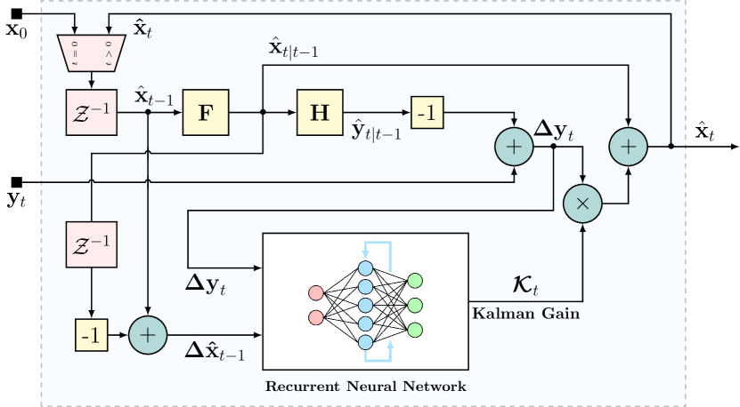
Fig. 1: kn block diagram.

3 Uncertainty in KalmanNet

kn, detailed in Subsection 2.2, is designed and trained to estimate the state variable $\mathbf{x}_{t}$. Neither its architecture nor the loss measure it uses for training encourage kn to maintain an estimate of its error covariance, which the kf provides. However, as we show here, the fact that kn preserves the flow of the kf allows to estimate its error covariance from its internal features.

3.1 Kalman Gain-based Error Covariance

To extend kn to provide uncertainty, we build on top of the interpretable feature of kn, which is the estimated kg. Combined with the observation model, the kg can be used to compute the time-dependent, error covariance matrix $\boldsymbol{\Sigma}_{t}$, thus bypassing the need to explicitly estimate the evolution model, as stated in the following theorem:

Theorem 1.

Consider the ss model (1) where $\mathbf{H}$ has full column rank; i.e., $\tilde{\mathbf{H}}=\left(\mathbf{H}^{\top}\cdot\mathbf{H}\right)^{-1}$ exists. Then, filtering with the kg $\mathbfcal{K}_{t}$ (3) results in estimation with error covariance

$${\boldsymbol{\Sigma}}_{t}=\left(\mathbf{I}_{m}-\mathbfcal{K}_{t}\cdot\mathbf{H}\right) \cdot\tilde{\mathbf{H}}\cdot\mathbf{H}^{\top}\left(\mathbf{I}_{n}-\mathbf{H}\cdot\mathbfcal{K}_{t}\right)^{-1}$$

$$\cdot\mathbf{H}\cdot\mathbfcal{K}_{t}\cdot\mathbf{H}\cdot\tilde{\mathbf{H}}.$$ (6)

Proof.

By combining (3) and (5), the error covariance can be written as ${\boldsymbol{\Sigma}}_{t}=\left(\mathbf{I}_{m}-\mathbfcal{K}_{t}\cdot\mathbf{H}\right){\boldsymbol{\Sigma}}_{t|t-1}$. Thus, to estimate ${\boldsymbol{\Sigma}}_{t}$, we express ${\boldsymbol{\Sigma}}_{t|t-1}$ using $\mathbfcal{K}_{t}$ and the available domain knowledge. To that end, multiplying (3) by $\mathbf{H}$ gives

$$\mathbf{H}\cdot\mathbfcal{K}_{t}=\mathbf{H}\cdot{\boldsymbol{\Sigma}}_{t\left|t-1\right.}\cdot{\mathbf{H}}^{\top}\cdot{\mathbf{S}}^{-1}_{t\left|t-1\right.}.$$ (7)

Next, (7) is multiplied by $\mathbf{S}_{t\left|t-1\right.}$ from the right side, followed by substitution of (2b), which yields

$$\mathbf{H}\cdot\mathbfcal{K}_{t}\cdot\left(\mathbf{H}\cdot\boldsymbol{\Sigma}_{t\left|t-1\right.}\cdot\mathbf{H}^{\top}+\mathbf{R}\right)=\mathbf{H}\cdot{\boldsymbol{\Sigma}}_{t\left|t-1\right.}\cdot{\mathbf{H}}^{\top}.$$ (8)

Combining terms in (8) results in

$$\mathbf{H}\cdot\boldsymbol{\Sigma}_{t\left|t-1\right.}\cdot\mathbf{H}^{\top}=\left(\mathbf{I}_{n}-\mathbf{H}\cdot\mathbfcal{K}_{t}\right)^{-1}\cdot\mathbf{H}\cdot\mathbfcal{K}_{t}.$$ (9)

Multiplying (9) from the left by $\mathbf{H}^{\top}$ and from the right by $\mathbf{H}$ yields $\mathbf{H}^{\top}\cdot\mathbf{H}\cdot\boldsymbol{\Sigma}_{t\left|t-1\right.}\cdot\mathbf{H}^{\top}\cdot\mathbf{H}=\mathbf{H}^{\top}\left(\mathbf{I}_{n}-\mathbf{H}\cdot\mathbfcal{K}_{t}\right)^{-1}\cdot\mathbf{H}\cdot\mathbfcal{K}_{t}\cdot\mathbf{H}$, which, when $\tilde{\mathbf{H}}=\left(\mathbf{H}^{\top}\cdot\mathbf{H}\right)^{-1}$ exists, results in

$$\boldsymbol{\Sigma}_{t\left|t-1\right.}=\tilde{\mathbf{H}}\cdot\mathbf{H}^{\top}\left(\mathbf{I}_{n}-\mathbf{H}\cdot\mathbfcal{K}_{t}\right)^{-1}\cdot\mathbf{H}\cdot\mathbfcal{K}_{t}\cdot\mathbf{H}\cdot\tilde{\mathbf{H}},$$ (10)

concluding the proof of the theorem. ∎

Theorem 1 indicates that when the observation model is known and $\mathbf{H}$ has full column rank—requiring that the number of measurements not be smaller than the number of tracked states—then one can extend kn to predict its error covariance alongside its state estimation. The resulting procedure is summarized as Algorithm 1.

3.2 Discussion

Init: Trained kn, previous estimate $\hat{\mathbf{x}}_{t-1}$, incoming observations $\mathbf{y}_{t}$;

1 Filtering: Apply kn to estimate $\hat{\mathbf{x}}_{t}$;

2 Error prediction: Estimate $\hat{\boldsymbol{\Sigma}}_{t}$ via (6) with $\mathbfcal{K}_{t}$ being the output of the internal rnn of kn;

Output: Predicted state $\hat{\mathbf{x}}_{t}$ and error $\hat{\boldsymbol{\Sigma}}_{t}$

Algorithm 1 kn with error prediction

kn [18] was designed for rt tracking in nl ss models with unknown noise statistics. Algorithm 1 extends it to provide not only $\hat{\mathbf{x}}_{t}$, an estimate of the state—i.e., for which it was previously derived and trained—but also $\hat{\boldsymbol{\Sigma}}_{t}$, an estimate of the time-dependent covariance matrix as an uncertainty measure. This is achieved since kn retains the interpretable flow of the mb kf, where the kg is learned by a dedicated rnn. Numerical evaluations presented in Section 4 indicate that kn computes the true covariance matrix as it reflects the true empirical error—as expected from the mse bias variance decomposition theorem [22].

For simplicity and clarity of exposition, Algorithm 1 was derived for linear ss models. In Section 4 we also present results for a nl chaotic system, where the extended kf derivation is used; i.e., the ss model matrices are replaced with their respecting Jacobians [2, Ch. 10]. The additional requirement—that observation noise covariance $\mathbf{R}$ is known and needed only for the purpose of estimating the covariance—is often satisfied, as in many applications the main modelling challenge is related to the state evolution rather than the measurement noise. Since we assume that we have access to a labeled ds, one can estimate $\mathbf{R}$ with standard techniques without assumptions regarding the evolution. The case where $\mathbf{H}$ is not full column rank is left for future work.

4 Numerical Evaluations

In this section we numerically compare the covarince computed by kn to the one computed by the kf in the linear and nl cases.

We start with the lg ss model, for which the kf achieves the mmse lower bound, and is an unbiased estimator [23]. We generate data from a scalar ss model where $\mathbf{H}=\mathbf{Q}=\mathbf{R}=1$ and $\mathbf{F}=0.9$, with sequence length of $100$ samples, and compare the error predicted by kn and its deviation from the true error to those computed by the mb kf that knows the ss model. We observe in Fig. 2 that the theoretical error computed by kf for each time step $t$ and the error predicted by kn coincide, and that both algorithms have a similar empirical error. In Fig. 3 we demonstrate that for a single realization of gt trajectory, both algorithms produce the same uncertainty bounds. Next, we consider the case where both kn and the mb kf are plugged in with a mismatched model parameter $\mathbf{F}=0.5$. In Figs. 4 and 5 we observe that for such a model mismatch, kn produces uncertainty similar to the empirical error, while the kf underestimates its empirical error.

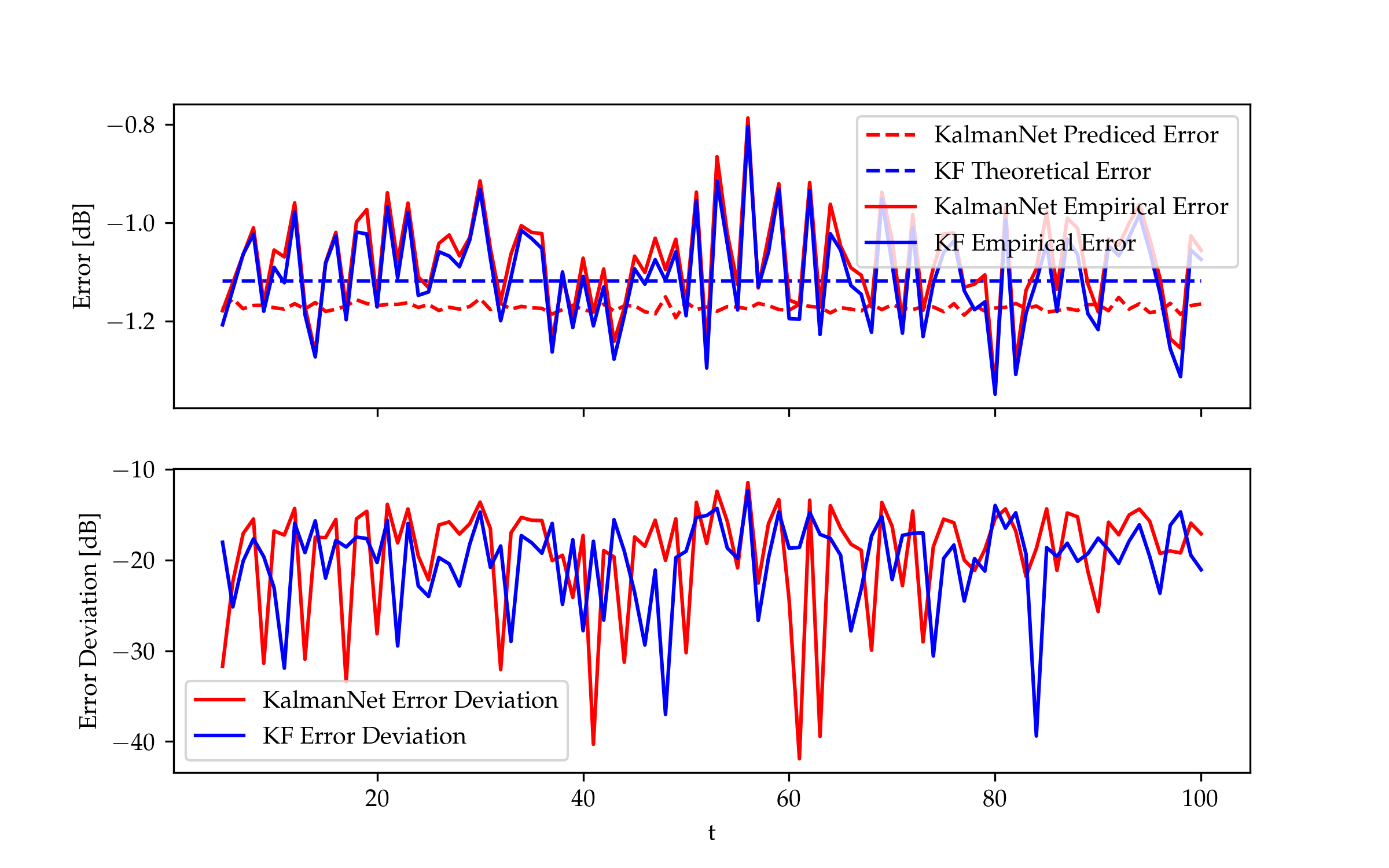
Fig. 2: Average error, linear ss model.

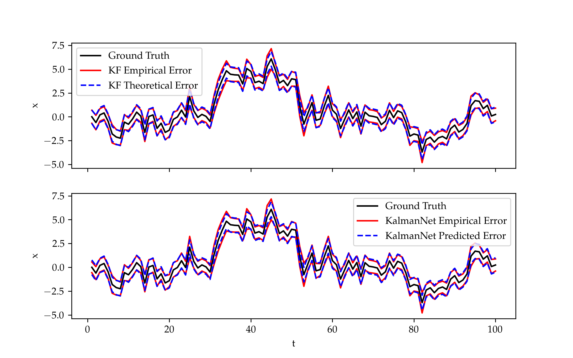
Fig. 3: Single trajectory, linear ss model.

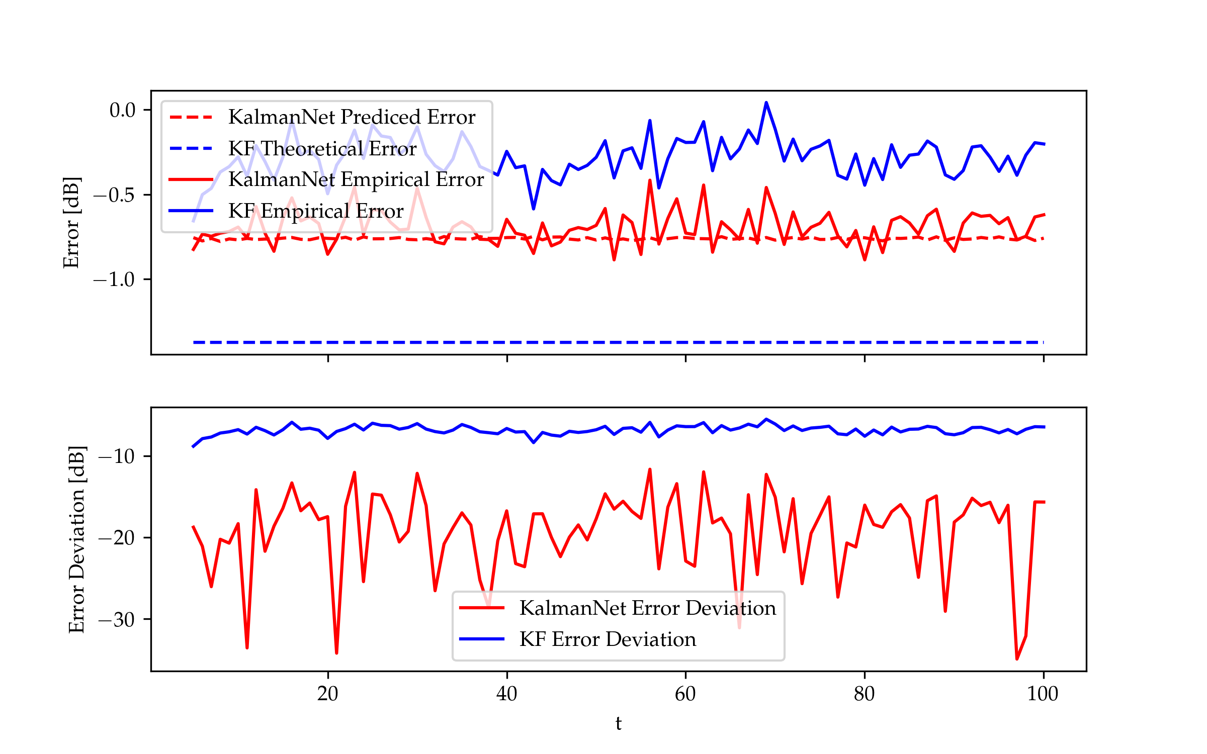
Fig. 4: Average error, linear ss model with mismatch.

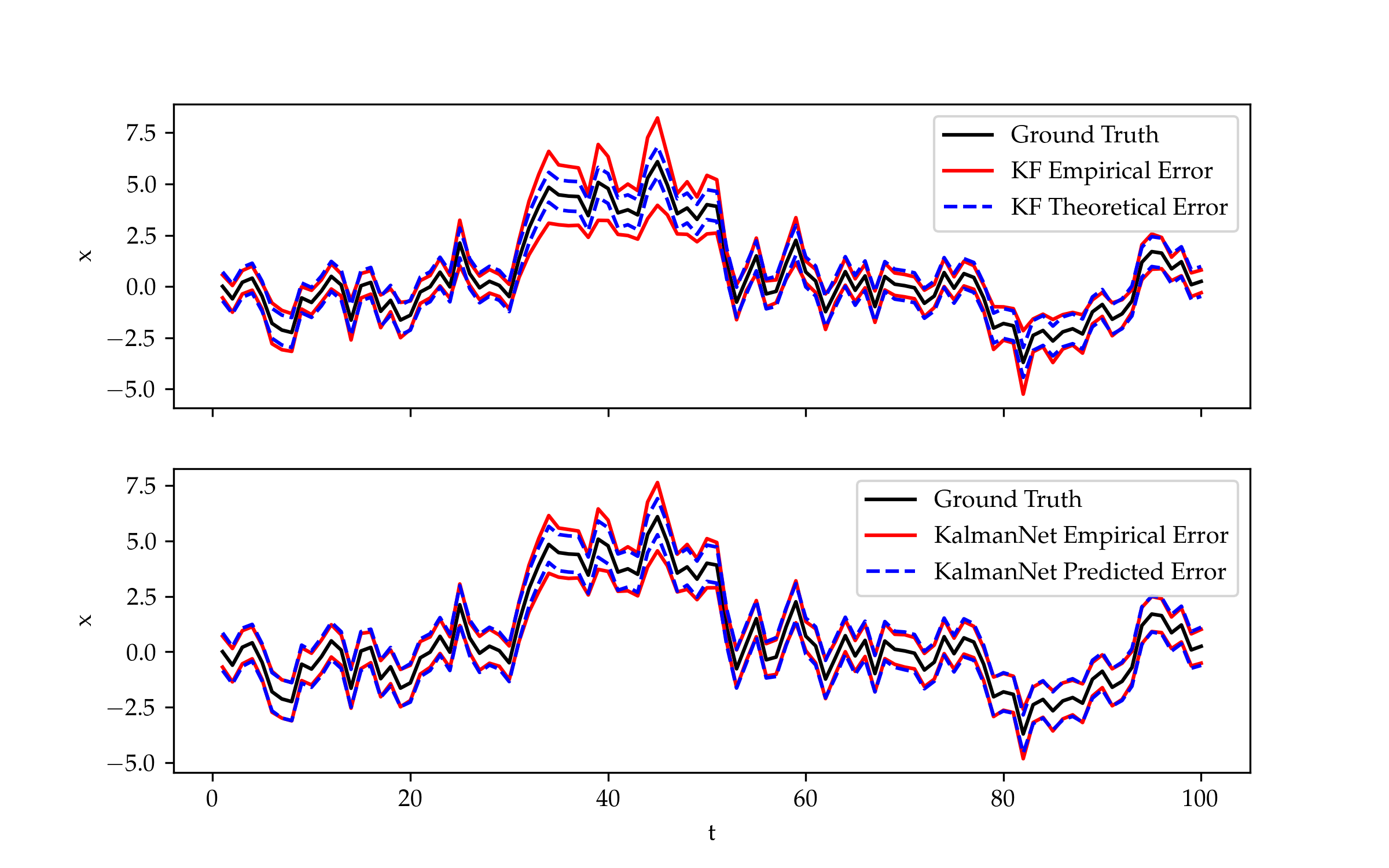
Fig. 5: Single trajectory, linear ss model with mismatch.

Next, we demonstrate the merits of kn when filtering the la—a challenging three-dimensional nl chaotic system—and compare its performance to the extended kf. See [18] for a detailed description of this setup. The model mismatch in this case is due to sampling a ct system characterized by differential equations to dt. In Fig. 6 we clearly observe that kn achieves a lower mse and estimates its error fairly accurately, while the extended kf overestimates it.

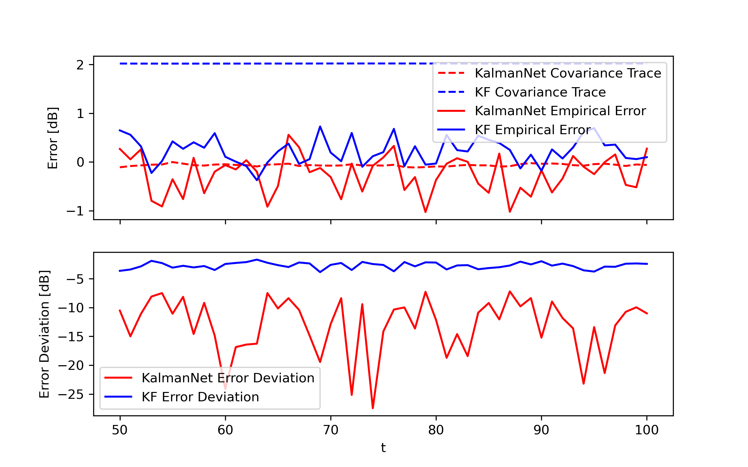
Fig. 6: Average error, nl la model.

5 Conclusions

In this work we extended the recently proposed kn state estimator to predict its error alongside the latent state. This is achieved by exploiting the hybrid mb/dd architecture of kn, which produces the kg as an internal feature. We prove that one can often utilize the learned kg to predict the error covariance as a measure of uncertainty. Our numerical results demonstrate that this extension allows kn to accurately predict both the state and error, improving upon the kf in the presence of model-mismatch and non-linearities.

References

- [1] Rudolph Emil Kalman, “A new approach to linear filtering and prediction problems,” Journal of Basic Engineering, vol. 82, no. 1, pp. 35–45, 1960.
- [2] James Durbin and Siem Jan Koopman, Time series analysis by state space methods, Oxford University Press, 2012.
- [3] Junyoung Chung, Caglar Gulcehre, KyungHyun Cho, and Yoshua Bengio, “Empirical evaluation of gated recurrent neural networks on sequence modeling,” preprint arXiv:1412.3555, 2014.
- [4] Ashish Vaswani, Noam Shazeer, Niki Parmar, Jakob Uszkoreit, Llion Jones, Aidan N Gomez, Lukasz Kaiser, and Illia Polosukhin, “Attention is all you need,” preprint arXiv:1706.03762, 2017.
- [5] Philipp Becker, Harit Pandya, Gregor Gebhardt, Cheng Zhao, C James Taylor, and Gerhard Neumann, “Recurrent Kalman networks: Factorized inference in high-dimensional deep feature spaces,” in International Conference on Machine Learning, 2019, pp. 544–552.
- [6] Manzil Zaheer, Amr Ahmed, and Alexander J Smola, “Latent LSTM allocation: Joint clustering and non-linear dynamic modeling of sequence data,” in International Conference on Machine Learning, 2017, pp. 3967–3976.
- [7] Anh Nguyen, Jason Yosinski, and Jeff Clune, “Deep neural networks are easily fooled: High confidence predictions for unrecognizable images,” in Proceedings of the IEEE conference on computer vision and pattern recognition, 2015, pp. 427–436.
- [8] Matteo Poggi, Fabio Tosi, and Stefano Mattoccia, “Quantitative evaluation of confidence measures in a machine learning world,” in Proceedings of the IEEE International Conference on Computer Vision, 2017, pp. 5228–5237.
- [9] Ian Osband, Zheng Wen, Mohammad Asghari, Morteza Ibrahimi, Xiyuan Lu, and Benjamin Van Roy, “Epistemic neural networks,” preprint arXiv:2107.08924, 2021.
- [10] Laurent Valentin Jospin, Wray Buntine, Farid Boussaid, Hamid Laga, and Mohammed Bennamoun, “Hands-on Bayesian neural networks–a tutorial for deep learning users,” preprint arXiv:2007.06823, 2020.
- [11] Maximilian Karl, Maximilian Soelch, Justin Bayer, and Patrick Van der Smagt, “Deep variational Bayes filters: Unsupervised learning of state space models from raw data,” preprint arXiv:1605.06432, 2016.
- [12] Rahul Krishnan, Uri Shalit, and David Sontag, “Structured inference networks for nonlinear state space models,” in Proceedings of the AAAI Conference on Artificial Intelligence, 2017, vol. 31.
- [13] Christian Naesseth, Scott Linderman, Rajesh Ranganath, and David Blei, “Variational sequential Monte Carlo,” in International Conference on Artificial Intelligence and Statistics. PMLR, 2018, pp. 968–977.
- [14] Pieter Abbeel, Adam Coates, Michael Montemerlo, Andrew Y Ng, and Sebastian Thrun, “Discriminative training of Kalman filters,” in Robotics: Science and Systems, 2005, vol. 2, p. 1.
- [15] Tuomas Haarnoja, Anurag Ajay, Sergey Levine, and Pieter Abbeel, “Backprop KF: Learning discriminative deterministic state estimators,” in Advances in Neural Information Processing Systems, 2016, pp. 4376–4384.
- [16] Bracha Laufer-Goldshtein, Ronen Talmon, and Sharon Gannot, “A hybrid approach for speaker tracking based on TDOA and data-driven models,” IEEE/ACM Trans. Audio, Speech, Language Process., vol. 26, no. 4, pp. 725–735, 2018.
- [17] Liang Xu and Ruixin Niu, “EKFNet: Learning system noise statistics from measurement data,” in Proc. IEEE ICASSP, 2021, pp. 4560–4564.
- [18] Guy Revach, Nir Shlezinger, Xiaoyong Ni, Adria Lopez Escoriza, Ruud JG van Sloun, and Yonina C Eldar, “KalmanNet: Neural network aided Kalman filtering for partially known dynamics,” preprint arXiv:2107.10043, 2021.
- [19] Nir Shlezinger, Jay Whang, Yonina C Eldar, and Alexandros G Dimakis, “Model-based deep learning,” preprint arXiv:2012.08405, 2020.
- [20] Adrià López Escoriza, Guy Revach, Nir Shlezinger, and Ruud J G van Sloun, “Data-driven Kalman-based velocity estimation for autonomous racing,” in Proc. IEEE ICAS, 2021.
- [21] Yaakov Bar-Shalom, X Rong Li, and Thiagalingam Kirubarajan, Estimation with applications to tracking and navigation: Theory algorithms and software, John Wiley & Sons, 2004.
- [22] Jerome Friedman, Trevor Hastie, and Robert Tibshirani, The elements of statistical learning, vol. 1, Springer series in Statistics, New York, 2001.
- [23] Jeffrey Humpherys, Preston Redd, and Jeremy West, “A fresh look at the Kalman filter,” SIAM Review, vol. 54, no. 4, pp. 801–823, 2012.