An SDP method for Fractional Semi-infinite Programming Problems with SOS-convex polynomials

Abstract.

In this paper, we study a class of fractional semi-infinite polynomial programming problems involving sos-convex polynomial functions. For such a problem, by a conic reformulation proposed in our previous work and the quadratic modules associated with the index set, a hierarchy of semidefinite programming (SDP) relaxations can be constructed and convergent upper bounds of the optimum can be obtained. In this paper, by introducing Lasserre’s measure-based representation of nonnegative polynomials on the index set to the conic reformulation, we present a new SDP relaxation method for the considered problem. This method enables us to compute convergent lower bounds of the optimum and extract approximate minimizers. Moreover, for a set defined by infinitely many sos-convex polynomial inequalities, we obtain a procedure to construct a convergent sequence of outer approximations which have semidefinite representations (SDr). The convergence rate of the lower bounds and outer SDr approximations are also discussed.

1. Introduction

The fractional semi-infinite polynomial programming (FSIPP) problem considered in this paper is in the following form:

$$\left\{\begin{aligned} r^{\star}:=\min_{x\in{\mathbb{R}}^{m}}&\ \frac{f(x)}{g(x)}\\ \text{s.t.}&\ \varphi_{1}(x)\leq 0,\ldots,\varphi_{s}(x)\leq 0,\\ &\ p(x,y)\leq 0,\ \ \forall y\in\mathbf{Y}\subset{\mathbb{R}}^{n},\end{aligned}\right.$$ (FSIPP)

where $f,g$, $\varphi_{1},\ldots,\varphi_{s}\in{\mathbb{R}}[x]$ and $p\in{\mathbb{R}}[x,y]$. Here, ${\mathbb{R}}[x]$ (resp. ${\mathbb{R}}[x,y]$) denotes the ring of real polynomials in $x=(x_{1},\ldots,x_{m})$ (resp., $x=(x_{1},\ldots,x_{m})$ and $y=(y_{1},\ldots,y_{n})$). We denote by $\mathbf{K}$ and $\mathbf{S}$ the feasible set and the set of optimal solutions of (FSIPP), respectively. In this paper, we assume that $\mathbf{S}\neq\emptyset$ and consider the following assumptions on (FSIPP): A1: (i) $\mathbf{Y}\subseteq[-1,1]^{n}$ and is closed; (ii) $\varphi_{j}$, $j=1,\ldots,s,$ $p(\cdot,y)$, $y\in\mathbf{Y}$ are all sos-convex;
A2: (i) $f$, $-g$ are both sos-convex; (ii) Either $f(x)\geq 0$ and $g(x)>0$ for all $x\in\mathbf{K}$, or $g(x)$ is affine and $g(x)>0$ for all $x\in\mathbf{K}.$

A convex polynomial is called sos-convex if its Hessian matrix can be written as the product of a polynomial matrix and its transpose (see Definition 2.1). In particular, separable convex polynomials and convex quadratic functions are sos-convex. Therefore, our model (FSIPP) under A1-2 contains subclasses of linear semi-infinite programming and convex quadratic semi-infinite programming with polynomial parametrizations. Moreover, if $\mathbf{Y}$ is defined by finitely many polynomial inequalities, then the problem of minimizing a polynomial $h(y)\in{\mathbb{R}}[y]$ over $\mathbf{Y}$ can be reformulated as an FSIPP problem satisfying A1-2. As is well known, the polynomial optimization problem is NP-hard even when $n>1$, $h(y)$ is a nonconvex quadratic polynomial and $\mathbf{Y}$ is a polytope (c.f. [38]). Hence, in general the FSIPP problem considered in this paper cannot be expected to be solved in polynomial time unless P=NP. Particularly, minimizing a ratio of quadratic functions is of great importance and some methods can be found in [21, 46, 49]. However, these methods were given for dealing with finitely constrained problems, while we aim to solve the problem (FSIPP) with infinitely many constraints.

Over the last several decades, due to a great number of applications in many fields, semi-infinite programming (SIP) has attracted a great deal of interest and been very active research areas [12, 13, 19, 32]. Numerically, SIP problems can be solved by different approaches including, for instance, discretization methods, local reduction methods, exchange methods, simplex-like methods etc; see [12, 19, 32] and the references therein for details. If the functions involved in SIP are polynomials, the representations of nonnegative polynomials over semi-algebraic sets from real algebraic geometry allow us to derive semidefinite programming (SDP) [47] relaxations for such problems [16, 27, 45, 48].

In our previous work [15], instead of sos-convexity, we deal with the FSIPP problems under convexity assumption. In [15], we first reformulate the FSIPP problem to a conic optimization problem. This conic reformulation, together with inner approximations with sums-of-square structures of the cone of nonnagative polynomials on $\mathbf{Y}$ (e.g. the quadratic modules [40] associated with $\mathbf{Y}$), enables us to derive a hierarchy of SDP relaxations of (FSIPP). Applying such appoach to (FSIPP) under sos-convexity assumption, we can obtain convergent upper bounds of $r^{\star}$. In this paper, we follow the methodology in [15] and present a new SDP method for (FSIPP) under A1-2. Instead of the quadratic modules associated with $\mathbf{Y}$, we introduce Lasserre’s measure-based representation of nonnegative polynomials on $\mathbf{Y}$ (c.f. [26]) to the conic reformulation of (FSIPP). With the new SDP method, we can compute convergent lower bounds of $r^{\star}$ and extract approximate minimizers of (FSIPP) in the case when $\mathbf{Y}$ is a simple set, like a box, a ball, a sphere, or a polytope.

We say that a convex set $C$ in ${\mathbb{R}}^{m}$ has a semidefinite representation (SDr) if there exist some integers $l,k$ and real $k\times k$ symmetric matrices $\{A_{i}\}_{i=0}^{m}$ and $\{B_{j}\}_{j=1}^{l}$ such that

$$C=\left\{x\in{\mathbb{R}}^{m}\ \Big{|}\ \exists w\in{\mathbb{R}}^{l},\ \text{s.t.}\ A_{0}+\sum_{i=1}^{m}A_{i}x_{i}+\sum_{j=1}^{l}B_{j}w_{j}\succeq 0\right\}.$$ (1)

Semidefinite representations of convex sets can help us to build SDP relaxations of many computationally intractable optimization problems. Arising from it, one of the basic issues in convex algebraic geometry is to characterize convex sets in ${\mathbb{R}}^{m}$ which are SDr sets and give systematic procedures to obtain their semidefinite representations (or arbitrarily close SDr approximations) [6, 14, 17, 18, 24, 28, 33]. Observe that the feasible set of (FSIPP) is a subset of ${\mathbb{R}}^{m}$ defined by infinitely many sos-convex polynomial inequalities. For a set of this form, applying the approach in our previous work [16], a convergent sequence of inner SDr approximations can be constructed. In this paper, from the new SDP relaxations of (FSIPP), we obtain a procedure to construct a convergent sequence of outer SDr approximations of such a set.

Remark that the main ingredient in our method to obtain the lower bounds of $r^{\star}$ and the outer SDr approximations of $\mathbf{K}$ is Lasserre’s measure-based representation of nonnegative polynomials on the index set [26]. For polynomial minimization problems which can be regarded as a special case of (FSIPP), the convergence rate of Lasserre’s measure-based upper bounds is well studied in [44] in difference situations. By combining the results in [44] and the metric regularity of semi-infinite convex inequality system (c.f. [7]), we derive some convergence analysis of the lower bounds of $r^{\star}$ and the outer SDr approximations of $\mathbf{K}$ obtained in this paper.

This paper is organized as follows. In Section 2, some notation and preliminaries are given. In Section 3, we present a hierarchy of SDP relaxations for the lower bounds of $r^{\star}$ and a procedure to construct a convergent sequence of outer SDr approximations of $\mathbf{K}$. The convergence rate of the lower bounds and outer SDr approximations is discussed in Section 4. Some numerical experiments are given in Section 5.

2. Preliminaries

In this section, we collect some notation and preliminary results which will be used in this paper. We denote by $x$ (resp., $y$) the $m$-tuple (resp., $n$-tuple) of variables $(x_{1},\ldots,x_{m})$ (resp., $(y_{1},\ldots,y_{n})$). The symbol $\mathbb{N}$ (resp., $\mathbb{R}$, ${\mathbb{R}}_{+}$) denotes the set of nonnegative integers (resp., real numbers, nonnegative real numbers). For any $t\in\mathbb{R}$, $\lceil t\rceil$ denotes the smallest integer that is not smaller than $t$. For $u\in\mathbb{R}^{m}$, $\|u\|$ denotes the standard Euclidean norm of $u$. For $\alpha=(\alpha_{1},\ldots,\alpha_{n})\in\mathbb{N}^{n}$, $|\alpha|=\alpha_{1}+\cdots+\alpha_{n}$. For $k\in\mathbb{N}$, denote $\mathbb{N}^{n}_{k}=\{\alpha\in\mathbb{N}^{n}\mid|\alpha|\leq k\}$ and $|\mathbb{N}^{n}_{k}|$ its cardinality. For variables $x\in\mathbb{R}^{m}$, $y\in\mathbb{R}^{n}$ and $\beta\in\mathbb{N}^{m},\alpha\in\mathbb{N}^{n}$, $x^{\beta}$, $y^{\alpha}$ denote $x_{1}^{\beta_{1}}\cdots x_{m}^{\beta_{m}}$, $y_{1}^{\alpha_{1}}\cdots y_{n}^{\alpha_{n}}$, respectively. ${\mathbb{R}}[x]$ (resp., $\mathbb{R}[y]$) denotes the ring of polynomials in $x$ (resp., $y$) with real coefficients. For $h\in{\mathbb{R}}[x]$ (resp. $\in{\mathbb{R}}[y]$), we denote by $\deg_{x}(h)$ (resp. $\deg_{y}(h)$) its (total) degree. For $k\in\mathbb{N}$, denote by ${\mathbb{R}}[x]_{k}$ (resp., ${\mathbb{R}}[y]_{k}$) the set of polynomials in ${\mathbb{R}}[x]$ (resp., ${\mathbb{R}}[y]$) of degree up to $k$. For $A={\mathbb{R}}[x],\ {\mathbb{R}}[y],\ {\mathbb{R}}[x]_{k},\ {\mathbb{R}}[y]_{k}$, denote by $A^{*}$ the dual space of linear functionals from $A$ to ${\mathbb{R}}$. Denote by $\mathbf{B}^{m}$ the unit ball in ${\mathbb{R}}^{m}$ and $\mathbf{B}^{m}_{r}(u)$ (resp., $\mathbf{B}^{m}_{r}$) the ball centered at $u$ (resp., the origin) in ${\mathbb{R}}^{m}$ with the radius $r$.

One of the difficulties in solving (FSIPP) is the feasibility test of a point $u\in{\mathbb{R}}^{m}$, which is caused by the infinitely many constraints $p(u,y)\leq 0$ for all $y\in\mathbf{Y}$. Thus, it is reasonable to study the representations of nonnegative polynomials on $\mathbf{Y}$. Denote

$$d_{y}:=\deg_{y}p(x,y)\quad\text{and}\quad\mathcal{P}_{d_{y}}(\mathbf{Y}):=\{h(y)\in{\mathbb{R}}[y]_{d_{y}}\mid h(y)\geq 0,\ \forall y\in\mathbf{Y}\}.$$

Now we recall the measure-based outer approximations of $\mathcal{P}_{d_{y}}(\mathbf{Y})$ proposed by Lasserre [26].

A polynomial $h\in{\mathbb{R}}[y]$ is said to be a sum-of-squares (sos) of polynomials if it can be written as $h=\sum_{i=1}^{l}h_{i}^{2}$ for some $h_{1},\ldots,h_{l}\in{\mathbb{R}}[y]$. The symbols $\Sigma^{2}[x]$ and $\Sigma^{2}[y]$ denote the sets of polynomials that are sum-of-squares of polynomials in ${\mathbb{R}}[x]$ and ${\mathbb{R}}[y]$, respectively. For each $k\in\mathbb{N}$, denote $\Sigma^{2}_{k}[x]:=\Sigma^{2}[x]\cap{\mathbb{R}}[x]_{2k}$ and $\Sigma^{2}_{k}[y]=\Sigma^{2}[y]\cap{\mathbb{R}}[y]_{2k}$, respectively. Note that for a given $h\in{\mathbb{R}}[y]$, checking if $h\in\Sigma^{2}_{k}[y]$ is an SDP feasibility problem. In fact, denote by $\mathbf{v}_{k}$ the column vector containing all monomials in ${\mathbb{R}}[y]$ of degree at most $k$. Then, $h\in\Sigma^{2}_{k}[y]$ if and only if there exists a positive semidefinite matrix $H\in{\mathbb{R}}^{|\mathbf{v}_{k}|\times|\mathbf{v}_{k}|}$ such that $h=\langle H,\mathbf{v}_{k}{\mathbf{v}_{k}}^{T}\rangle$ (c.f. [37]).

In the rest of this paper,

let $\nu$ be a fixed and finite Borel measure with support exactly $\mathbf{Y}$.

For each $k\in\mathbb{N}$, define

$$\mathcal{P}^{k}_{d_{y}}(\mathbf{Y}):=\left\{\psi(y)\in{\mathbb{R}}[y]_{d_{y}}\mid\int_{\mathbf{Y}}\psi(y)\sigma(y)\mathrm{d}\nu(y)\geq 0,\ \forall\sigma\in\Sigma^{2}_{k}[y]\right\}.$$ (2)

Then for each $k\in\mathbb{N}$, it is clear that $\mathcal{P}^{k}_{d_{y}}(\mathbf{Y})$ is a closed subset of ${\mathbb{R}}[y]_{d_{y}}$ and $\mathcal{P}^{k}_{d_{y}}(\mathbf{Y})\supset\mathcal{P}_{d_{y}}(\mathbf{Y})$.

To lighten the notation, throughout the rest of the paper, we abbreviate the notation $\mathcal{P}_{d_{y}}(\mathbf{Y})$ and $\mathcal{P}^{k}_{d_{y}}(\mathbf{Y})$ to $\mathcal{P}(\mathbf{Y})$ and $\mathcal{P}^{k}(\mathbf{Y})$, respectively.

Theorem 2.1.

[26, Theorem 3.2] Suppose that $\mathbf{Y}\subseteq[-1,1]^{n}$, then we have $\mathcal{P}^{k_{1}}(\mathbf{Y})\supset\mathcal{P}^{k_{2}}(\mathbf{Y})\supset\mathcal{P}(\mathbf{Y})$ for $k_{1}<k_{2}$ and $\mathcal{P}(\mathbf{Y})=\cap_{k=1}^{\infty}\mathcal{P}^{k}(\mathbf{Y})$.

Remark 2.1.

As proved in [26, Theorem 3.2], it is required that $\mathbf{Y}\subseteq[-1,1]^{n}$ for the convergence result in Theorem 2.1. That is why it is assumed in A1 which, however, can be fulfilled after a possible rescaling if $\mathbf{Y}$ is compact.

For a given $\psi\in{\mathbb{R}}[y]_{d_{y}}$, it is not hard to see that $\psi\in\mathcal{P}^{k}(\mathbf{Y})$ if and only if the matrix $\int_{\mathbf{Y}}\psi\mathbf{v}_{k}{\mathbf{v}_{k}}^{T}\mathrm{d}\nu(y)$ is positive semidefinite. Observe that each entry in the matrix $\int_{\mathbf{Y}}\psi\mathbf{v}_{k}\mathbf{v}_{k}^{T}\mathrm{d}\nu(y)$ is a linear combination of the coefficients of $\psi$. It implies that each $\mathcal{P}^{k}(\mathbf{Y})$ has an SDr with no lifting ($l=0$ in (1)) and thus checking if $\psi\in\mathcal{P}^{k}(\mathbf{Y})$ is an SDP feasibility problem. We emphasize that, to get the SDr of $\mathcal{P}^{k}(\mathbf{Y})$, we need compute effectively the integrals $\int_{\mathbf{Y}}y^{\beta}\mathrm{d}\nu(y)$, $\beta\in\mathbb{N}^{n}$. There are several interesting cases of $\mathbf{Y}$ where these integrals can be obtained either explicitly in closed form or numerically (see [26] and Section 5).

Now let us recall some background above sos-convex polynomials in ${\mathbb{R}}[x]$ introduced by Helton and Nie [18].

Definition 2.1.

[18] A polynomial $h\in{\mathbb{R}}[x]$ is sos-convex if there are an integer $r$ and a matrix polynomial $H\in{\mathbb{R}}[x]^{r\times m}$ such that the Hessian $\nabla^{2}h=H(x)^{T}H(x)$.

Clearly, an sos-convex polynomial is convex. However, the converse is not true. Ahmadi and Parrilo [4] proved that the set of convex polynomials and the set of sos-convex polynomials in ${\mathbb{R}}[x]_{k}$ coincide if and only if $m=1$ or $k=2$ or $(m,k)=(2,4)$. Thus, any convex quadratic function and any convex separable polynomial is an sos-convex polynomial. The significance of sos-convexity is that it can be checked numerically by solving an SDP problem (see [18]), while checking the convexity of a polynomial is generally NP-hard (c.f. [3]). Interestingly, an extended Jensen’s inequality holds for sos-convex polynomials.

Proposition 2.1.

[25, Theorem 2.6] Let $h\in{\mathbb{R}}[x]_{2d}$ be sos-convex, and let $\mathscr{L}\in({\mathbb{R}}[x]_{2d})^{*}$ satisfy $\mathscr{L}(1)=1$ and $\mathscr{L}(\sigma)\geq 0$ for every $\sigma\in\Sigma^{2}_{d}[x]$. Then,

$$\mathscr{L}(h(x))\geq h(\mathscr{L}(x_{1}),\ldots,\mathscr{L}(x_{m})).$$

The following result plays a significant role in this paper.

Lemma 2.1.

[18, Lemma 8] Let $h\in{\mathbb{R}}[x]$ be sos-convex. If $h(u)=0$ and $\nabla h(u)=0$ for some $u\in{\mathbb{R}}^{m},$ then $h$ is an sos polynonmial.

3. SDP relaxations of FSIPP

In this section, we first recall the conic reformulation of (FSIPP) proposed in our previous work [15]. This conic reformulation, together with inner approximations with sos structures of $\mathcal{P}(\mathbf{Y})$ (e.g., the quadratic modules [40] associated with $\mathbf{Y}$), allows us to derive a hierarchy of SDP relaxations of (FSIPP) and obtain convergent upper bounds of $r^{\star}$. As a complement, we apply in this paper the outer approximations $\mathcal{P}^{k}(\mathbf{Y})$ of $\mathcal{P}(\mathbf{Y})$ to the conic reformulation and get a new SDP relaxation method of (FSIPP) which can give us convergent lower bounds of $r^{\star}$. Moreover, we gain a convergent sequence of outer SDr approximations of $\mathbf{K}$.

3.1. Conic reformulation

In this subsection, let us recall the conic reformulation of (FSIPP) proposed in [15] which makes it possible to derive SDP relaxations of (FSIPP).

Consider the problem

$$\min_{x\in\mathbf{K}}\ \ f(x)-r^{\star}g(x).$$ (3)

Note that, under A1-2, (3) is clearly a convex semi-infinite programming problem and its optimal value is $0$. Denote by $\mathcal{M}(\mathbf{Y})$ the set of finite nonnegative measures supported on $\mathbf{Y}$. Then, the Lagrangian dual of (3) reads

$$\max_{\mu\in\mathcal{M}(\mathbf{Y}),\eta_{j}\geq 0}\inf_{x\in{\mathbb{R}}^{m}}L_{f,g}(x,\mu,\eta),$$ (4)

where

$$L_{f,g}(x,\mu,\eta):=f(x)-r^{\star}g(x)+\int_{\mathbf{Y}}p(x,y)\mathrm{d}\mu(y)+\sum_{j=1}^{s}\eta_{j}\varphi_{j}(x).$$ (5)

Consider the assumption that

A3: The Slater condition holds for $\mathbf{K}$, i.e., there exists $u\in\mathbf{K}$ such that $p(u,y)<0$ for all $y\in\mathbf{Y}$ and $\varphi_{j}(u)<0$ for all $j=1,\ldots,s$.

Proposition 3.1.

(c.f. [32, 42]) Under A1-3, then there exist $\mu^{\star}\in\mathcal{M}(\mathbf{Y})$ and $\eta^{\star}\in{\mathbb{R}}_{+}^{s}$ such that $\inf_{x\in{\mathbb{R}}^{m}}L_{f,g}(x,\mu^{\star},\eta^{\star})=0$. Moreover, $\mu^{\star}$ can be chosen as an atomic measure, i.e., $\mu^{\star}=\sum_{i=1}^{l}\lambda_{i}\zeta_{v_{i}}$ where $l\leq n$, each $\lambda_{i}>0$ and $\zeta_{v_{i}}$ is the Dirac measure at $v_{i}\in\mathbf{Y}$.

Let $d_{x}:=\deg_{x}(p(x,y))$ and

$$\mathbf{d}:=\lceil\max\{\deg(f),\deg(g),\deg(\psi_{1}),\ldots,\deg(\psi_{s}),\deg_{x}(p(x,y))\}/2\rceil.$$ (6)

For $\mathscr{L}\in({\mathbb{R}}[x])^{*}$ (resp., $\mathscr{H}\in({\mathbb{R}}[y])^{*}$), denote by $\mathscr{L}(p(x,y))$ (resp., $\mathscr{H}(p(x,y))$) the image of $\mathscr{L}$ (resp., $\mathscr{H}$) on $p(x,y)$ regarded as an element in ${\mathbb{R}}[x]$ (resp., ${\mathbb{R}}[y]$) with coefficients in ${\mathbb{R}}[y]$ (resp., ${\mathbb{R}}[x]$), i.e., $\mathscr{L}(p(x,y))\in{\mathbb{R}}[y]$ (resp., $\mathscr{H}(p(x,y))\in{\mathbb{R}}[x]$).

Consider the following conic optimization problem

$$\qquad\left\{\begin{aligned} \hat{r}:=\sup_{\rho,\mathscr{H},\eta}\ &\rho&\\ \text{s.t.}\ &f(x)-\rho g(x)+\mathscr{H}(p(x,y))+\sum_{j=1}^{s}\eta_{j}\varphi_{j}(x)\in\Sigma_{\mathbf{d}}^{2}[x],&\\ &\rho\in{\mathbb{R}},\ \mathscr{H}\in(\mathcal{P}(\mathbf{Y}))^{*},\ \eta\in{\mathbb{R}}_{+}^{s}.&\end{aligned}\right.$$ (7)

Proposition 3.2.

Under A1-3, we have $\hat{r}=r^{\star}$.

Proof.

Let (atomic) $\mu^{\star}\in\mathcal{M}(\mathbf{Y})$ and $\eta^{\star}\in{\mathbb{R}}_{+}^{s}$ be the dual variables in Proposition 3.1. Define $\mathscr{H}^{\star}\in({\mathbb{R}}[y])^{*}$ by letting $\mathscr{H}^{\star}(y^{\beta})=\int_{\mathbf{Y}}y^{\beta}d\mu^{\star}(y)$ for any $\beta\in\mathbb{N}^{n}$. Then, $\mathscr{H}^{\star}\in(\mathcal{P}(\mathbf{Y}))^{*}$. Since $\mu^{\star}$ is atomic, it is easy to see that $L_{f,g}(x,\mu^{\star},\eta^{\star})$ is sos-convex under A1-2. Then, Lemma 2.1 implies that $L_{f,g}(x,\mu^{\star},\eta^{\star})\in\Sigma_{\mathbf{d}}^{2}[x]$. Therefore, $(r^{\star},\mathscr{H}^{\star},\eta^{\star})$ is feasible to (7) and $\hat{r}\geq r^{\star}$. On the other hand, for any $u^{\star}\in\mathbf{S}$ and any $(\rho,\mathscr{H},\eta)$ feasible to (7), it holds that

$$f(u^{\star})-\rho g(u^{\star})+\mathscr{H}(p(u^{\star},y))+\sum_{j=1}^{s}\eta_{j}\psi_{j}(u^{\star})\geq 0.$$

Then, the feasibility of $u^{\star}$ to (FSIPP) implies that $r^{\star}=\frac{f(u^{\star})}{g(u^{\star})}\geq\rho$ and thus $r^{\star}\geq\hat{r}$. ∎

Remark 3.1.

In view of the proof of Proposition 3.2, if we replace $\Sigma_{\mathbf{d}}^{2}[x]$ in (7) by any convex cone $\mathcal{C}[x]\subset{\mathbb{R}}[x]$ satisfying the condition

$$\Sigma_{\mathbf{d}}^{2}[x]\subseteq\mathcal{C}[x]\quad\text{and there exists }u^{\star}\in\mathbf{S}\ \text{such that }h(u^{\star})\geq 0\ \text{for all }h\in\mathcal{C}[x],$$

we still have $\hat{r}=r^{\star}$. ∎

If we substitute $\mathcal{P}(\mathbf{Y})$ in (7) by its approximations with sos structures, then (7) can be reduced to SDP problems and becomes tractable. In particular, if we replace $\mathcal{P}(\mathbf{Y})$ by the quadratic modules [40] generated by the defining polynomials of $\mathbf{Y}$, which are inner approximations of $\mathcal{P}(\mathbf{Y})$, we can obtain upper bounds of $r^{\star}$ from the resulting SDP relaxations. See [15] for more details. Our goal in this paper is to compute convergent lower bounds of $r^{\star}$ by SDP relaxations derived from (7). It will be done by substituting $\mathcal{P}(\mathbf{Y})$ with the outer approximations $\mathcal{P}^{k}(\mathbf{Y})$ in (2).

3.2. SDP relaxations for lower bounds of $r^{\star}$

In the rest of this paper, let us fix a suffciently large $\mathfrak{R}>0$ and a sufficiently small $g^{\star}>0$ such that

$$\|u^{\star}\|\leq\mathfrak{R}\quad\text{and}\quad g(u^{\star})\geq g^{\star}\quad\text{for some}\quad u^{\star}\in\mathbf{S}.$$ (8)

See [15, Remark 4.1] for the choice of $\mathfrak{R}$ and $g^{\star}$ in some circumstances. Let

$$Q=\{q_{1}(x):=\mathfrak{R}^{2}-\|x\|^{2},\ \ q_{2}(x):=g(x)-g^{\star}\},$$

and

$$\mathbf{M}_{\mathbf{d}}(Q):=\left\{\sum_{j=0}^{2}\sigma_{j}q_{j}\ \Big{|}\ q_{0}=1,\ \sigma_{j}\in\Sigma^{2}[x],\,\deg(\sigma_{j}q_{j})\leq 2\mathbf{d},\ j=0,1,2\right\},$$

i.e., $\mathbf{M}_{\mathbf{d}}(Q)$ be the $\mathbf{d}$-th quadratic module generated by $Q$ [40]. By Remark 3.1, we still have $\hat{r}=r^{\star}$ if we replace $\Sigma^{2}_{\mathbf{d}}[x]$ by $\mathbf{M}_{\mathbf{d}}(Q)$ in (7).

Consider the following problem, where we replace $\Sigma^{2}_{\mathbf{d}}[x]$ and $\mathcal{P}(\mathbf{Y})$ in (7) by $\mathbf{M}_{\mathbf{d}}(Q)$ and $\mathcal{P}^{k}(\mathbf{Y})$, respectively,

$$\qquad\left\{\begin{aligned} r_{k}^{\mbox{\tiny primal}}:=\sup_{\rho,\mathscr{H},\eta}\ &\rho&\\ \text{s.t.}\ &f(x)-\rho g(x)+\mathscr{H}(p(x,y))+\sum_{j=1}^{s}\eta_{j}\varphi_{j}(x)\in\mathbf{M}_{\mathbf{d}}(Q),&\\ &\rho\in{\mathbb{R}},\ \mathscr{H}\in\left(\mathcal{P}^{k}(\mathbf{Y})\right)^{*},\ \eta\in{\mathbb{R}}_{+}^{s}.&\end{aligned}\right. \mathrm{P}_{k}$$ ()

Its Lagrangian dual reads

$$\qquad\left\{\begin{aligned} r_{k}^{\mbox{\tiny dual}}:=\inf_{\mathscr{L}\in({\mathbb{R}}[x]_{2\mathbf{d}})^{*}}\ &\mathscr{L}(f)&\\ \text{s.t.}\ &\mathscr{L}\in(\mathbf{M}_{\mathbf{d}}(Q))^{*},\ \mathscr{L}(g)=1,&\\ &-\mathscr{L}(p(x,y))\in\mathcal{P}^{k}(\mathbf{Y}),\ \mathscr{L}(\varphi_{j})\leq 0,\ j=1,\ldots,s.\end{aligned}\right. \mathrm{D}_{k}$$ ()

For each $k\in\mathbb{N}$, recall that checking if $-\mathscr{L}(p(x,y))\in\mathcal{P}^{k}(\mathbf{Y})$ for a given $\mathscr{L}\in({\mathbb{R}}[x]_{2\mathbf{d}})^{*}$ is an SDP feasibility problem. Therefore, computing $r^{\mbox{\tiny primal}}_{k}$ and $r^{\mbox{\tiny dual}}_{k}$ is reduced to solving a pair of an SDP problem and its dual. We omit the detail for simplicity. In the following, we will show that $\{r_{k}^{\mbox{\tiny primal}}\}_{k\in\mathbb{N}}$ and $\{r_{k}^{\mbox{\tiny dual}}\}_{k\in\mathbb{N}}$ are convergent lower bounds of $r^{\star}$, and we can extract approximate minimizers of (FSIPP) from the SDP relaxations ($\mathrm{D}_{k}$). To this end, we first point out that the feasible set of the ($\mathrm{D}_{k}$) is uniformly bounded.

Proposition 3.3.

For any $\mathscr{L}\in({\mathbb{R}}[x]_{2\mathbf{d}})^{*}$ satisfying that $\mathscr{L}(\sigma_{0})\geq 0$ for any $\sigma_{0}\in\Sigma^{2}_{\mathbf{d}}[x]$ and $\mathscr{L}((\mathfrak{R}^{2}-\|x\|^{2})\sigma)\geq 0$ for any $\sigma\in\Sigma^{2}_{\mathbf{d}-1}[x]$, we have

$$\|(\mathscr{L}(x^{\alpha}))_{\alpha\in\mathbb{N}^{m}_{2\mathbf{d}}}\|\leq\mathscr{L}(1)\sqrt{\binom{m+\mathbf{d}}{m}}\sum_{i=0}^{\mathbf{d}}\mathfrak{R}^{2i}.$$

Consequently, for any $k\in\mathbb{N}$ and any $\mathscr{L}_{k}\in({\mathbb{R}}[x]_{2\mathbf{d}})^{*}$ feasible to ($\mathrm{D}_{k}$),

$$\|(\mathscr{L}_{k}(x^{\alpha}))_{\alpha\in\mathbb{N}^{m}_{2\mathbf{d}}}\|\leq\frac{1}{g^{\star}}\sqrt{\binom{m+\mathbf{d}}{m}}\sum_{i=0}^{\mathbf{d}}\mathfrak{R}^{2i}.$$

Proof.

For any $\mathscr{L}\in({\mathbb{R}}[x]_{2\mathbf{d}})^{*}$ satisfying that $\mathscr{L}(\sigma_{0})\geq 0$ for any $\sigma_{0}\in\Sigma^{2}_{\mathbf{d}}[x]$ and $\mathscr{L}((\mathfrak{R}^{2}-\|x\|^{2})\sigma)\geq 0$ for any $\sigma\in\Sigma^{2}_{\mathbf{d}-1}[x]$, by [20, Lemma 3] and its proof, it holds that

$$\sqrt{\sum_{\alpha\in\mathbb{N}^{m}_{2\mathbf{d}}}\left(\mathscr{L}(x^{\alpha})\right)^{2}}\leq\mathscr{L}(1)\sqrt{\binom{m+\mathbf{d}}{m}}\sum_{i=0}^{\mathbf{d}}\mathfrak{R}^{2i}.$$

For any $\mathscr{L}_{k}\in({\mathbb{R}}[x]_{2\mathbf{d}})^{*}$ feasible to ($\mathrm{D}_{k}$), we have $\mathscr{L}_{k}(g-g^{\star})\geq 0$ and $\mathscr{L}_{k}(g)=1$. Hence, $\mathscr{L}_{k}(1)\leq\mathscr{L}_{k}(g)/g^{\star}=1/g^{\star}$. The conlusion follows. ∎

The following theorem states that we can compute convergent lower bounds of $r^{\star}$ and extract approximate minimizers of (FSIPP) from the SDP relaxations ($\mathrm{P}_{k}$) and ($\mathrm{D}_{k}$). For any $\mathscr{L}\in({\mathbb{R}}[x]_{2\mathbf{d}})^{*}$, denote

$$\mathscr{L}(x):=(\mathscr{L}(x_{1}),\ldots,\mathscr{L}(x_{m}))\in{\mathbb{R}}^{m}.$$

Theorem 3.1.

Under A1-3, it holds that

1. $r^{\mbox{\tiny primal}}_{k}=r^{\mbox{\tiny dual}}_{k}\leq r^{\star}$ and $r^{\mbox{\tiny dual}}_{k}$ is attainable for each $k\in\mathbb{N}$;

2. $\lim_{k\rightarrow\infty}r^{\mbox{\tiny primal}}_{k}=\lim_{k\rightarrow\infty}r^{\mbox{\tiny dual}}_{k}=r^{\star}$;

3. For any convergent subsequence $\{\mathscr{L}^{\star}_{k_{i}}(x)/\mathscr{L}^{\star}_{k_{i}}(1)\}_{i}$ $($always exists$)$ of $\{\mathscr{L}^{\star}_{k}(x)/\mathscr{L}^{\star}_{k}(1)\}_{k}$ where $\mathscr{L}_{k}^{\star}$ is a minimizer of ($\mathrm{D}_{k}$), we have $\lim_{i\rightarrow\infty}\mathscr{L}^{\star}_{k_{i}}(x)/\mathscr{L}^{\star}_{k_{i}}(1)\in\mathbf{S}$. Consequently, if $\mathbf{S}$ is singleton, then $\lim_{k\rightarrow\infty}\mathscr{L}^{\star}_{k}(x)/\mathscr{L}^{\star}_{k}(1)$ is the unique minimizer of (FSIPP).

Proof.

(i) Fix a $u^{\star}\in\mathbf{S}$ satisfying (8) and define a linear functional $\mathscr{L}^{\star}\in({\mathbb{R}}[x]_{2\mathbf{d}})^{*}$ by letting $\mathscr{L}^{\star}(x^{\alpha})=\frac{(u^{\star})^{\alpha}}{g(u^{\star})}$ for each $\alpha\in\mathbb{N}^{m}_{2\mathbf{d}}$. By the definition of $\mathbf{M}_{\mathbf{d}}(Q)$ and $\mathcal{P}^{k}(\mathbf{Y})$, as well as Theorem 2.1, it is easy to see that $\mathscr{L}^{\star}$ is feasible to ($\mathrm{D}_{k}$) for each $k\in\mathbb{N}$. Then,

$$r^{\mbox{\tiny dual}}_{k}\leq\mathscr{L}^{\star}(f)=\frac{f(u^{\star})}{g(u^{\star})}=r^{\star}.$$

Then for any $k\in\mathbb{N}$, by Proposition 3.3, the feasible set of ($\mathrm{D}_{k}$) is nonempty, uniformly bounded and closed. Hence, the solution set of ($\mathrm{D}_{k}$) is nonempty and bounded, which implies that ($\mathrm{P}_{k}$) is strictly feasible (c.f. [43, Section 4.1.2]). Consequently, the strong duality $r_{k}^{\mbox{\tiny primal}}=r_{k}^{\mbox{\tiny dual}}$ holds by [43, Theorem 4.1.3].

Now we show (ii) and (iii) together. Let $\{\mathscr{L}^{\star}_{k}\}_{k\in\mathbb{N}}\subset({\mathbb{R}}[x]_{2\mathbf{d}})^{*}$ be a sequence such that $\mathscr{L}^{\star}_{k}$ is a minimizer of ($\mathrm{D}_{k}$) for each $k\in\mathbb{N}$. As $\{\mathscr{L}^{\star}_{k}(x^{\alpha})_{\alpha\in\mathbb{N}^{m}_{2\mathbf{d}}}\}_{k}$ is uniformly bounded by Proposition 3.3, there is a subsequence $\{\mathscr{L}^{\star}_{k_{i}}\}_{k_{i}}$ and a $\mathscr{L}^{\star}\in({\mathbb{R}}[x]_{2\mathbf{d}})^{*}$ such that $\lim_{i\rightarrow\infty}\mathscr{L}^{\star}_{k_{i}}(x^{\alpha})=\mathscr{L}^{\star}(x^{\alpha})$ for all $\alpha\in\mathbb{N}^{m}_{2\mathbf{d}}$. Because the sequence $\{r_{k}^{\mbox{\tiny dual}}\}_{k}$ is monotone nondecreasing and bounded by $r^{\star}$ as $k\rightarrow\infty$ , the limit of $\{r_{k}^{\mbox{\tiny dual}}\}_{k}$ exists and $\mathscr{L}^{\star}(f)=\lim_{k\rightarrow\infty}r_{k}^{\mbox{\tiny dual}}$. Moreover, from the pointwise convergence, we get the following: (a) $\mathscr{L}^{\star}\in(\mathbf{M}_{\mathbf{d}}(Q))^{*}$; (b) $\mathscr{L}^{\star}(g)=1$; (c) $-\mathscr{L}^{\star}(p(x,y))\in\cap_{k=1}^{\infty}\mathcal{P}^{k}(\mathbf{Y})$; (d) $\mathscr{L}^{\star}(\varphi_{j})\leq 0$ for $j=1,\ldots,s$. In particular, (c) holds because $\mathcal{P}^{k}(\mathbf{Y})$ is closed in ${\mathbb{R}}[y]_{d_{y}}$ and $\mathcal{P}^{k_{2}}(\mathbf{Y})\subseteq\mathcal{P}^{k_{1}}(\mathbf{Y})$ for $k_{1}<k_{2}$. We have $\mathscr{L}^{\star}(1)>0$. In fact, $\mathscr{L}^{\star}(1)\geq 0$ since $\mathscr{L}^{\star}\in(\Sigma^{2}_{\mathbf{d}}[x])^{*}$ by (a). If $\mathscr{L}^{\star}(1)=0$, then by Proposition 3.3, we have $\mathscr{L}^{\star}(x^{\alpha})=0$ for all $\alpha\in\mathbb{N}^{m}_{2\mathbf{d}}$, which contradicts (b). From (c) and Theorem 2.1, we get $-\mathscr{L}^{\star}(p(x,y))\in\mathcal{P}(\mathbf{Y})$. Then, for any $y\in\mathbf{Y}$, by Proposition 2.1,

$$p\left(\frac{\mathscr{L}^{\star}(x)}{\mathscr{L}^{\star}(1)},y\right)\leq\frac{1}{\mathscr{L}^{\star}(1)}\mathscr{L}^{\star}(p(x,y))\leq 0,$$

For the same reason, (d) implies that

$$\psi_{j}\left(\frac{\mathscr{L}^{\star}(x)}{\mathscr{L}^{\star}(1)}\right)\leq 0,\ \ j=1,\ldots,s,$$

which shows that $\mathscr{L}^{\star}(x)/\mathscr{L}^{\star}(1)\in\mathbf{K}$. Since $f(x)$ and $-g(x)$ are also sos-convex, under A2, we have

$$r^{\star}\leq\frac{f\left(\frac{\mathscr{L}^{\star}(x)}{\mathscr{L}^{\star}(1)}\right)}{g\left(\frac{\mathscr{L}^{\star}(x)}{\mathscr{L}^{\star}(1)}\right)}\leq\frac{\frac{1}{\mathscr{L}^{\star}(1)}\mathscr{L}^{\star}(f)}{\frac{1}{\mathscr{L}^{\star}(1)}\mathscr{L}^{\star}(g)}=\mathscr{L}^{\star}(f)=\lim_{k\rightarrow\infty}r_{k}^{\mbox{\tiny dual}}\leq r^{\star}.$$

It implies that $\frac{\mathscr{L}^{\star}(x)}{\mathscr{L}^{\star}(1)}\in\mathbf{S}$ and $\lim_{k\rightarrow\infty}r^{\mbox{\tiny primal}}_{k}=\lim_{k\rightarrow\infty}r^{\mbox{\tiny dual}}_{k}=r^{\star}$.

Assume that $\mathbf{S}$ is singleton and let $\mathbf{S}=\{u^{\star}\}$. The above arguments show that $\lim_{i\rightarrow\infty}\mathscr{L}^{\star}_{k_{i}}(x)/\mathscr{L}^{\star}_{k_{i}}(1)=u^{\star}$ for any convergent subsequence of $\{\mathscr{L}^{\star}_{k}(x)/\mathscr{L}^{\star}_{k}(1)\}_{k}$ which is bounded. Hence, the whole sequence $\{\mathscr{L}^{\star}_{k}(x)/\mathscr{L}^{\star}_{k}(1)\}_{k}$ converges to $u^{\star}$ as $k$ tends to $\infty$. ∎

Remark 3.2.

From its proof, we can see that Theorem 3.1 (i) still holds provided only A1-(i) and the existence of $u^{\star}\in\mathbf{S}$ satisfying (8), while the convexity of $f$, $-g$, $\varphi_{j}$’s and $p(\cdot,y)$, $y\in\mathbf{Y}$, is not necessary.

3.3. Outer SDr approximations of $\mathbf{K}$

Observe that the feasible set $\mathbf{K}$ of (FSIPP) is defined by infinitely many sos-convex polynomial inequalities. For a set of this form, applying the approach in our previous work [16], a convergent sequence of inner SDr approximations can be constructed. This appoach relies on the sos representation of the Lagrangian function $L_{f,g}(x,\mu^{\star},\eta^{\star})$ and the quadratic modules associated with $\mathbf{Y}$. Next, we show that a convergent sequence of outer SDr approximations of $\mathbf{K}$ can be constructed from the SDP relaxations ($\mathrm{D}_{k}$). For each $k\in\mathbb{N}$, define

$$\Lambda_{k}:=\left\{\mathscr{L}(x)\in{\mathbb{R}}^{m}:\left\{\begin{aligned} &\mathscr{L}(\sigma_{0})\geq 0,\ \forall\ \sigma_{0}\in\Sigma^{2}_{\mathbf{d}}[x],\\ &\mathscr{L}((\mathfrak{R}^{2}-\|x\|^{2})\sigma)\geq 0,\ \forall\ \sigma\in\Sigma^{2}_{\mathbf{d}-1}[x],\\ &-\mathscr{L}(p(x,y))\in\mathcal{P}^{k}(\mathbf{Y}),\ \mathscr{L}(1)=1,\\ &\mathscr{L}(\varphi_{j})\leq 0,\ j=1,\ldots,s.\end{aligned}\right.\right\}.$$ (9)

It is easy to see that $\Lambda_{k}$ is indeed an SDr set for each $k\in\mathbb{N}$.

Theorem 3.2.

Under A1, we have $\mathbf{K}\cap\mathbf{B}^{m}_{\mathfrak{R}}\subseteq\Lambda_{k_{2}}\subseteq\Lambda_{k_{1}}\subseteq\mathbf{B}^{m}_{\mathfrak{R}}$ for $k_{1}<k_{2}$ and $\mathbf{K}\cap\mathbf{B}^{m}_{\mathfrak{R}}=\cap_{k=1}^{\infty}\Lambda_{k}$. Consequently, if $\mathbf{K}$ is compact and $\mathfrak{R}$ is large enough such that $\mathbf{K}\subset\mathbf{B}^{m}_{\mathfrak{R}}$, then $\mathbf{K}=\cap_{k=1}^{\infty}\Lambda_{k}$.

Proof.

It is clear that $\Lambda_{k_{2}}\subseteq\Lambda_{k_{1}}$ for $k_{1}<k_{2}$. For any $u\in\mathbf{K}\cap\mathbf{B}^{m}_{\mathfrak{R}}$, let $\mathscr{L}^{\prime}\in({\mathbb{R}}[x]_{2\mathbf{d}})^{*}$ be such that $\mathscr{L}^{\prime}(x^{\alpha})=u^{\alpha}$ for each $\alpha\in\mathbb{N}^{m}_{2\mathbf{d}}$. Then by Theorem 2.1, $\mathscr{L}^{\prime}$ satisfies the conditions in (9) and hence $u\in\Lambda_{k}$ for each $k\in\mathbb{N}$. Assume that $\mathscr{L}\in({\mathbb{R}}[x]_{2\mathbf{d}})^{*}$ satisfies the conditions in (9) . As the function $\|x\|^{2}$ is sos-convex, by Proposition 2.1,

$$\|\mathscr{L}(x)\|^{2}\leq\mathscr{L}(\|x\|^{2})\leq\mathscr{L}(\mathfrak{R}^{2})=\mathfrak{R}^{2}\cdot\mathscr{L}(1)=\mathfrak{R}^{2}.$$

Hence, $\Lambda_{k}\subseteq\mathbf{B}^{m}_{\mathfrak{R}}$ for all $k\in\mathbb{N}$.

It remains to prove that $\cap_{k=1}^{\infty}\Lambda_{k}\subseteq\mathbf{K}$. Fix a point $u\in\cap_{k=1}^{\infty}\Lambda_{k}$. Then for each $k\in\mathbb{N}$, there exsits a $\mathscr{L}_{k}\in({\mathbb{R}}[x]_{2\mathbf{d}})^{*}$ satisfying the conditions in (9) and $\mathscr{L}_{k}(x)=u$. By Proposition 3.3, the vector $(\mathscr{L}_{k}(x^{\alpha}))_{\alpha\in\mathbb{N}^{m}_{2\mathbf{d}}}$ is uniformly bounded for all $k\in\mathbb{N}$. Then there exists a convergent subsequence $\{\mathscr{L}_{k_{i}}\}_{i}$ and a $\widetilde{\mathscr{L}}\in({\mathbb{R}}[x]_{2\mathbf{d}})^{*}$ such that $\lim_{i\rightarrow\infty}\mathscr{L}_{k_{i}}(x^{\alpha})=\widetilde{\mathscr{L}}(x^{\alpha})$ for each $\alpha\in\mathbb{N}^{m}_{2\mathbf{d}}$. By the pointwise convergence, we obtain that (a) $\widetilde{\mathscr{L}}(\sigma)\geq 0$ for all $\sigma\in\Sigma^{2}_{\mathbf{d}}[x]$; (b) $\widetilde{\mathscr{L}}(1)=1$; (c) $-\widetilde{\mathscr{L}}(p(x,y))\in\mathcal{P}^{k}(\mathbf{Y})$ for each $k\in\mathbb{N}$; (d) $\widetilde{\mathscr{L}}(\varphi_{j})\leq 0,\ j=1,\ldots,s.$ By (c) and Theorem 2.1, $-\widetilde{\mathscr{L}}(p(x,y))\in\mathcal{P}(\mathbf{Y})$. Then for any $y\in\mathbf{Y}$, by the sos-convexity of $p(x,y)$ in $x$, (a), (b) and Proposition 2.1 again,

$$p(u,y)=p(\widetilde{\mathscr{L}}(x),y)\leq\widetilde{\mathscr{L}}(p(x,y))\leq 0.$$

For the same reason, we have $\varphi_{j}(u)\leq 0$ for $j=1,\ldots,s$. We can conclude that $u\in\mathbf{K}$. ∎

Remark 3.3.

In [28, 33], some tractable methods using SDP are proposed to approximate semialgebraic sets defined with quantifiers. Clearly, the set $\mathbf{K}$ studied in this paper is in such a case with a universal quantifier. The method in [28, 33] works for $\mathbf{K}$ in a general form without requiring $-p(x,y)$ to be convex in $x$ and approximates $\mathbf{K}$ by a sequence of sublevel sets of a single polynomial. Different from that, we construct convergent SDr approximations of $\mathbf{K}$ by fully exploiting the sos-convexity of the defining polynomials.∎

3.4. Some discussions

Typically, lower bounds of semi-infinite programming problems can be computed by the discretization method by grids (see [19]). Compared with other numerical methods for general semi-infinite programming problems, this method can avoid globally solving the lower level problem $\max_{y\in\mathbf{Y}}p(u,y)$ to test the feasibility of a point $u\in{\mathbb{R}}^{m}$, which could be very hard and is one of the main computational problems in semi-infinite programming.

Precisely, for (FSIPP), we can replace $\mathbf{Y}$ by $\mathbf{Y}\cap T$ where $T\subset[-1,1]^{n}$ is a fixed grid, and solve the resulting finitely constrained problem

$$\left\{\begin{aligned} \min_{x\in{\mathbb{R}}^{m}}&\ \frac{f(x)}{g(x)}\\ \text{s.t.}&\ \varphi_{1}(x)\leq 0,\ldots,\varphi_{s}(x)\leq 0,\\ &\ p(x,y)\leq 0,\ \ \forall y\in\mathbf{Y}\cap T.\end{aligned}\right.$$ (10)

We suppose that the Hausdorff distance between $\mathbf{Y}$ and $\mathbf{Y}\cap T$ tends to $0$ as the grid size of $T$ vanishes. Denote by $\mathbf{K}_{T}$ the feasible set of (10). Then, under A2-(ii), we can assume that the grid size of $T$ is small enough and hence $g(x)>0$ on $\mathbf{K}_{T}$. In fact, for a fixed $u\in{\mathbb{R}}^{m}$ with $g(u)\leq 0$, if $\varphi_{i}(u)\leq 0$ for all $i=1,\ldots,s$, then there must be a point $\bar{y}\in\mathbf{Y}$ such that $p(u,\bar{y})>0$ because of A2-(ii). As the grid size of $T$ is small enough, there exists a point $\hat{y}\in\mathbf{Y}\cap T$ close to $\bar{y}$ such that $p(u,\hat{y})>0$ which implies that $u\not\in\mathbf{K}_{T}$.

We can consider the following three ways to solve (10) in the case when $g(x)$ is affine. In this case, as $g(x)>0$ on $\mathbf{K}_{T}$, it is not hard to check that $\frac{f(x)}{g(x)}$ is strictly quasiconvex on $\mathbf{K}_{T}$ under A1-2. That is, for any $u,v\in\mathbf{K}_{T}$,

$$\frac{f(u)}{g(u)}<\frac{f(v)}{g(v)}\quad\text{implies}\quad\frac{f(\lambda_{1}u+\lambda_{2}v)}{g(\lambda_{1}u+\lambda_{2}v)}<\frac{f(v)}{g(v)}\quad\text{for any}\quad\lambda_{1},\lambda_{2}>0\quad\text{with}\quad\lambda_{1}+\lambda_{2}=1.$$

Hence, the first way to solve (10), as a quasiconvex optimization problem, is by using bisection method with each step a convex feasibility problem. Second, since any local minimizer of (10) is also a global one (c.f. [39, Theorem 2]) due to the strict quasiconvexity of $\frac{f(x)}{g(x)}$ on $\mathbf{K}_{T}$, any local or global methods (e.g. interior-point methods, SQP methods, etc.) for solving general constrained nonlinear programming can be applied to (10). Third, we can also reformulate (10) to an SDP problem under the assumption that the Slater condition holds for (10). In fact, as $g(x)>0$ on $\mathbf{K}_{T}$, (10) is equivalent to

$$\max_{r\in{\mathbb{R}}}\ r\quad\text{s.t.}\quad f(x)-rg(x)\geq 0\quad\text{for all}\quad x\in\mathbf{K}_{T}.$$

Since $g(x)$ is affine, $f(x)-rg(x)$ is sos-convex for any $r\in{\mathbb{R}}$. Then, the convex positivstellensatz [25, Theorem 3.3] implies that (10) can be equivalently reformulated to

$$\left\{\begin{aligned} \max_{r\in{\mathbb{R}}}&\ r\\ \text{s.t.}&\ f(x)-rg(x)=\sigma+\sum_{i=1}^{s}\lambda_{i}\varphi_{i}(x)+\sum_{y\in\mathbf{Y}\cap T}\eta_{y}p(x,y),\\ &\ \sigma\in\Sigma^{2}_{\mathbf{d}}[x],\ \lambda_{i}\geq 0,\ i=1,\ldots,s,\ \eta_{y}\geq 0,\ y\in\mathbf{Y}\cap T,\end{aligned}\right.$$ (11)

which in fact is an SDP problem. Note that the number of nonnegative variables $\eta_{y}$ is equal to the cardinality of $\mathbf{Y}\cap T$.

Convergent lower bounds of $r^{\star}$ can be obtained by solving (10) provided that mesh size of the expansive sequence of grids tends to zero. However, in general, it is challenging to generate effcient grids for such a task. For a large $n$, if we use the regular grids

$$T_{N}:=\left\{-1+\frac{2}{N}i\right\}_{i=0,\ldots,N}\times\cdots\times\left\{-1+\frac{2}{N}i\right\}_{i=0,\ldots,N}\subset[-1,1]^{n},\quad N\in\mathbb{N},$$ (12)

the rapidly increasing grid points in $\mathbf{Y}$ as $N$ increases cause the resulting problems more and more intractable. See Example 5.2 for a comparison of our SDP method with the above discretization scheme.

To end this section, we consider the possibility of applying the diagonally dominant sum of squares (dsos) and scaled diagonally dominant sum of squares (sdsos) structures [1, 2, 34]to ($\mathrm{P}_{k}$) for handling (FSIPP) problems with large numbers $m$ and $\mathbf{d}$. For such problems, the sos structures in the quadratic module $\mathbf{M}_{\mathbf{d}}(Q)$ give rise to semidefinite constraints of very large size in ($\mathrm{P}_{k}$) and ($\mathrm{D}_{k}$), even when the order $k$ is small. In view of the capability of the state-of-the-art SDP solvers, it can cause the resulting SDP problems very hard to solve or even intractable. In this case, we may impose the dsos and sdsos structures into ($\mathrm{P}_{k}$) to trade off computation time with lower bound quality.

A symmetric matrix $A=(a_{ij})$ is diagonally dominant (dd) if $a_{ii}\geq\sum_{j\neq i}|a_{ij}|$ for all $i$. A symmetric matrix $A$ is scaled diagonally dominant (sdd) if there exists a diagonal matrix $D$, with positive diagonal entries, such that $DAD$ is diagonally dominant. A polynomial $h\in{\mathbb{R}}[x]$ of degree $2d$ is dsos (resp. sdsos) if and only if it admits a representation as $h(x)=z^{T}(x)Hz(x)$, where $z(x)$ is the standard monomial vector of degree $\leq d$ in ${\mathbb{R}}[x]$ and $H$ is a dd (resp. sdd) matrix. We denote the set of polynomials in ${\mathbb{R}}[x]_{2d}$ that are dsos (resp. sdsos) by $DSOS_{m,2d}$ (resp. $SDSOS_{m,2d}$). It is clear that $DSOS_{m,2d}\subseteq SDSOS_{m,2d}\subseteq\Sigma_{d}^{2}[x]$. In general, all these containment relationships are strict. Notice that optimization over $DSOS_{m,2d}$ (resp. $SDSOS_{m,2d}$) can be done with a linear program (resp. second-order cone program) of size polynomial in $m$ (see [2, Theorem 3.9]).

Now we replace the sos structure in the quadratic module $\mathbf{M}_{\mathbf{d}}(Q)$ by dsos and sdsos structures, respectively, and define the following cones

$$\mathbf{M}_{\mathbf{d}}^{\mbox{\tiny dsos}}(Q):=\left\{\sum_{j=0}^{2}\sigma_{j}q_{j}\ \Big{|}\ q_{0}=1,\ \sigma_{j}\text{ is dsos},\,\deg(\sigma_{j}q_{j})\leq 2\mathbf{d},\ j=0,1,2\right\},$$

and

$$\mathbf{M}_{\mathbf{d}}^{\mbox{\tiny sdsos}}(Q):=\left\{\sum_{j=0}^{2}\sigma_{j}q_{j}\ \Big{|}\ q_{0}=1,\ \sigma_{j}\text{ is sdsos},\,\deg(\sigma_{j}q_{j})\leq 2\mathbf{d},\ j=0,1,2\right\}.$$

Clearly, it holds that

$$\mathbf{M}_{\mathbf{d}}^{\mbox{\tiny dsos}}(Q)\subseteq\mathbf{M}_{\mathbf{d}}^{\mbox{\tiny sdsos}}(Q)\subseteq\mathbf{M}_{\mathbf{d}}(Q).$$

Replacing $\mathbf{M}_{\mathbf{d}}(Q)$ in ($\mathrm{P}_{k}$) by $\mathbf{M}_{\mathbf{d}}^{\mbox{\tiny dsos}}(Q)$ and $\mathbf{M}_{\mathbf{d}}^{\mbox{\tiny sdsos}}(Q)$, respectively, we obtain

$$\qquad\left\{\begin{aligned} r_{k}^{\mbox{\tiny dsos}}:=\sup_{\rho,\mathscr{H},\eta}\ &\rho&\\ \text{s.t.}\ &f(x)-\rho g(x)+\mathscr{H}(p(x,y))+\sum_{j=1}^{s}\eta_{j}\varphi_{j}(x)\in\mathbf{M}_{\mathbf{d}}^{\mbox{\tiny dsos}}(Q),&\\ &\rho\in{\mathbb{R}},\ \mathscr{H}\in\left(\mathcal{P}^{k}(\mathbf{Y})\right)^{*},\ \eta\in{\mathbb{R}}_{+}^{s},&\end{aligned}\right. \mathrm{P}^{\mbox{\tiny dsos}}_{k}$$ ()

and

$$\qquad\left\{\begin{aligned} r_{k}^{\mbox{\tiny sdsos}}:=\sup_{\rho,\mathscr{H},\eta}\ &\rho&\\ \text{s.t.}\ &f(x)-\rho g(x)+\mathscr{H}(p(x,y))+\sum_{j=1}^{s}\eta_{j}\varphi_{j}(x)\in\mathbf{M}_{\mathbf{d}}^{\mbox{\tiny sdsos}}(Q),&\\ &\rho\in{\mathbb{R}},\ \mathscr{H}\in\left(\mathcal{P}^{k}(\mathbf{Y})\right)^{*},\ \eta\in{\mathbb{R}}_{+}^{s}.&\end{aligned}\right. \mathrm{P}^{\mbox{\tiny sdsos}}_{k}$$ ()

It is obvious that $r_{k}^{\mbox{\tiny dsos}}\leq r_{k}^{\mbox{\tiny sdsos}}\leq r_{k}^{\mbox{\tiny primal}}\leq r^{\star}$ for each $k\in\mathbb{N}$, even in absence of the convexity assumption in A1-2 (see Remark 3.2). It is remarkable that the semidefinite constraints brought by $\mathbf{M}_{\mathbf{d}}(Q)$ in ($\mathrm{P}_{k}$) are replaced by a set of linear inequality constraints (resp. second-order cone constraints) in ($\mathrm{P}^{\mbox{\tiny dsos}}_{k}$) (resp. ($\mathrm{P}^{\mbox{\tiny sdsos}}_{k}$)). Although the convergence of $\{r_{k}^{\mbox{\tiny dsos}}\}_{k\in\mathbb{N}}$ (resp. $\{r_{k}^{\mbox{\tiny sdsos}}\}_{k\in\mathbb{N}}$) to $r^{\star}$ is not guaranteed, the computation time for solving ($\mathrm{P}^{\mbox{\tiny dsos}}_{k}$) (resp. ($\mathrm{P}^{\mbox{\tiny sdsos}}_{k}$)) could be considerably less than that of ($\mathrm{P}_{k}$). Consequently, for (FSIPP) problems with large $m$ and $\mathbf{d}$ that are significantly beyond the capability of the SDP relaxation ($\mathrm{P}_{k}$), we can still expect to obtain meaningful lower bounds of $r^{\star}$ in a reasonable time by solving the alternatives ($\mathrm{P}^{\mbox{\tiny dsos}}_{k}$) or ($\mathrm{P}^{\mbox{\tiny sdsos}}_{k}$) (see Example 5.3).

4. Convergence rate analysis

In this section, we consider the convergence rate of the lower bound $r^{\mbox{\tiny dual}}_{k}$ to the optimal value $r^{\star}$ and the outer approximation $\Lambda_{k}$ to the feasible set $\mathbf{K}$. This will be done by combining the convergence analysis of Lasserre’s measure-based upper bounds for polynomial minimization problems in [44] and the metric regularity of semi-infinite convex inequality system (c.f. [7]). In this section, to apply the results in [44], we assume that the measure $\nu$ (2) is the Lebesgue measure with support exactly $\mathbf{Y}$.

Define the set-valued mapping $\mathcal{G}:\ {\mathbb{R}}^{m}\ \rightrightarrows\ {\mathbb{R}}^{2}$ by

$$\mathcal{G}(x):=\{(\eta,R)\in{\mathbb{R}}^{2}\mid\|x\|\leq R,\ p(x,y)\leq\eta,\ \forall\ y\in\mathbf{Y}\}.$$

Let $\mathbf{F}:=\{x\in{\mathbb{R}}^{m}\mid\varphi_{i}(x)\leq 0,\ i=1,\ldots,s\}$. Then, it is clear that $\mathbf{K}\cap\mathbf{B}^{m}_{\mathfrak{R}}=\mathcal{G}^{-1}(0,\mathfrak{R})\cap\mathbf{F}$.

Proposition 4.1.

[7, Lemma 3] The following statements are equivalent:

1. there exists $\bar{x}\in{\mathbb{R}}^{m}$ such that $\|\bar{x}\|<\bar{R}$ and $p(\bar{x},y)<\bar{\eta}$ for all $y\in\mathbf{Y}$;

2. $\mathcal{G}$ is metrically regular at any $u\in\mathcal{G}^{-1}(\bar{\eta},\bar{R})$ for $(\bar{\eta},\bar{R})$, i.e., there exist $d_{1},d_{2}>0$ and $c\geq 0$ such that whenever $\|x-u\|<d_{1}$ and $\|(\eta,R)-(\bar{\eta},\bar{R})\|<d_{2}$, it holds that

   $$\text{\rm dist}(x,\ \mathcal{G}^{-1}(\eta,R))\leq c\cdot\text{\rm dist}((\eta,R),\ \mathcal{G}(x)).$$

Consider the assumption that

A4: There exists $\bar{x}\in{\mathbb{R}}^{m}$ such that $\|\bar{x}\|<\mathfrak{R}$ and $p(\bar{x},y)<0$ for all $y\in\mathbf{Y}$.

Corollary 4.1.

Under A4, there exist $d>0$ and $c\geq 0$ such that whenever $\|x\|\leq\mathfrak{R}$ and $\text{\rm dist}(x,\ \mathcal{G}^{-1}(0,\mathfrak{R}))<d$, it holds that

$$\text{\rm dist}(x,\ \mathcal{G}^{-1}(0,\mathfrak{R}))\leq c\cdot\max\left\{\max_{y\in\mathbf{Y}}p(x,y),\ 0\right\}.$$

Proof.

Note that for any $x\in{\mathbb{R}}^{m}$ with $\|x\|\leq\mathfrak{R}$, $(\max_{y\in\mathbf{Y}}p(x,y),\mathfrak{R})\in\mathcal{G}(x)$. Then, for any $u\in\mathcal{G}^{-1}(0,\mathfrak{R})$, by A4 and Proposition 4.1, there exist $d_{u}>0$ and $c_{u}\geq 0$ such that whenever $\|x-u\|<d_{u}$ and $\|x\|\leq\mathfrak{R}$, it holds that

$$\text{\rm dist}(x,\ \mathcal{G}^{-1}(0,\mathfrak{R})) \leq c_{u}\cdot\text{\rm dist}((0,\mathfrak{R}),\ \mathcal{G}(x))$$ (13)

$$\leq c_{u}\cdot\max\left\{\max_{y\in\mathbf{Y}}p(x,y),\ 0\right\}.$$

As $\mathcal{G}^{-1}(0,\mathfrak{R})$ is compact, we can find finitely many points $u^{(i)}\in\mathcal{G}^{-1}(0,\mathfrak{R})$ and corresponding $d_{u^{(i)}}>0,\ c_{u^{(i)}}\geq 0$, $i=1,\ldots,t$, satisfying (13) and

$$\mathcal{G}^{-1}(0,\mathfrak{R})\subset\cup_{i=1}^{t}\{x\in{\mathbb{R}}^{m}\mid\|x-u^{(i)}\|<d_{u^{(i)}}\}=:\mathcal{O}.$$

Moreover, there exists $d>0$ such that

$$\{x\in{\mathbb{R}}^{m}\mid\text{\rm dist}(x,\ \mathcal{G}^{-1}(0,\mathfrak{R}))<d\}\subset\mathcal{O}.$$

Otherwise, there exists a sequence $\{x^{(k)}\}_{k\in\mathbb{N}}$ such that $\text{\rm dist}(x^{(k)},\ \mathcal{G}^{-1}(0,\mathfrak{R}))<\frac{1}{k}$ and $x^{(k)}\not\in\mathcal{O}$ for each $k\in\mathbb{N}$. As $\mathcal{G}^{-1}(0,\mathfrak{R})$ is compact, we can assume that there is a point $x^{\prime}\in{\mathbb{R}}^{m}$ such that $\lim_{k\rightarrow\infty}x^{(k)}=x^{\prime}$. Then, $\text{\rm dist}(x^{\prime},\ \mathcal{G}^{-1}(0,\mathfrak{R}))=0$ and hence $x^{\prime}\in\mathcal{G}^{-1}(0,\mathfrak{R})$. However, as $\mathcal{O}$ is open, we have $x^{\prime}\not\in\mathcal{O}$, a contradiction. Then, the conclusion holds for this $d>0$ and $c=\max_{1\leq i\leq t}c_{u^{(i)}}$. ∎

For any $\mathscr{L}_{k}\in({\mathbb{R}}[x]_{2\mathbf{d}})^{*}$, $k\in\mathbb{N}$, satisfying the conditions in (9), we define a number $E(\mathscr{L}_{k}):=\tilde{p}^{\star}_{k}-p^{\star}_{k}$, where

$$p^{\star}_{k}: =\min_{y\in\mathbf{Y}}-\mathscr{L}_{k}(p(x,y))$$ (14)

$$=\min_{\mu\in\mathcal{M}(Y)}\int_{\mathbf{Y}}-\mathscr{L}_{k}(p(x,y))\mathrm{d}\mu(y)\quad\text{s.t. }\int_{\mathbf{Y}}\mathrm{d}\mu(y)=1,$$

and

$$\left\{\begin{aligned} \tilde{p}^{\star}_{k}:=\min_{\sigma}&\ \int_{\mathbf{Y}}-\mathscr{L}_{k}(p(x,y))\sigma(y)\mathrm{d}y\\ \text{s.t.}&\ \sigma(y)\in\Sigma^{2}_{k}[y],\ \int_{\mathbf{Y}}\sigma(y)\mathrm{d}y=1.\end{aligned}\right.$$ (15)

In fact, (15) is the $k$-th Lasserre’s measure-based relaxation (see [26]) of (14), where the probability measures are replaced by the one having a density $\sigma\in\Sigma^{2}_{k}[y]$ with respect to the Lebesgue measure. Thus, $\tilde{p}^{\star}_{k}$ is an upper bound of $p^{\star}_{k}$ and $E(\mathscr{L}_{k})\geq 0$. By the definition of $\mathcal{P}^{k}(\mathbf{Y})$, we have $\tilde{p}^{\star}_{k}\geq 0$. Hence, it holds that

$$\max_{y\in\mathbf{Y}}\mathscr{L}_{k}(p(x,y))=-p_{k}^{\star}=E(\mathscr{L}_{k})-\tilde{p}^{\star}_{k}\leq E(\mathscr{L}_{k}).$$

Clearly, $\mathscr{L}_{k}^{\star}/\mathscr{L}_{k}^{\star}(1)\in({\mathbb{R}}[x]_{2\mathbf{d}})^{*}$ satisfies the conditions in (9) for any minmizer $\mathscr{L}_{k}^{\star}$ of ($\mathrm{D}_{k}$).

Theorem 4.1.

Under A1 and A4, there exist $k^{\prime}\in\mathbb{N}$ and $c\geq 0$ such that whenever $k\geq k^{\prime}$,

$$\text{\rm dist}(\mathscr{L}_{k}(x),\ \mathbf{K}\cap\mathbf{B}^{m}_{\mathfrak{R}})\leq c\cdot E(\mathscr{L}_{k}),$$ (16)

for any $\mathscr{L}_{k}$ satisfying the conditions in (9). Furthermore, under A1-4, there exists $\tilde{c}\geq 0$ such that whenever $k\geq k^{\prime}$,

$$0\leq r^{\star}-r^{\mbox{\tiny dual}}_{k}\leq\tilde{c}\cdot E(\mathscr{L}_{k}^{\star}/\mathscr{L}_{k}^{\star}(1)),$$

where $\mathscr{L}_{k}^{\star}$ is any minimizer of ($\mathrm{D}_{k}$).

Proof.

Let $d,\ c$ be the numbers in Corollary 4.1. By Theorem 3.2, the nested compact sets $\{\Lambda_{k}\}_{k\in\mathbb{N}}$ converges to $\mathbf{K}\cap\mathbf{B}^{m}_{\mathfrak{R}}$ as $k\to\infty$ in the Hausdorff sense. So there exists $k^{\prime}\in\mathbb{N}$ such that whenever $k\geq k^{\prime}$, $\text{\rm dist}(\mathscr{L}_{k}(x),\ \mathbf{K}\cap\mathbf{B}^{m}_{\mathfrak{R}})<d$ for any $\mathscr{L}_{k}$ satisfying the conditions in (9).

For any $\mathscr{L}_{k}$ satisfying the conditions in (9), as $\varphi_{i}(x)$, $p(x,y)$ is sos-convex in $x$ for all $i=1,\ldots,s$, $y\in\mathbf{Y}$, Proposition 2.1 implies that

$$\varphi(\mathscr{L}_{k}(x))\leq\mathscr{L}_{k}(\varphi)\leq 0,\quad i=1,\ldots,s,$$

$$p(\mathscr{L}_{k}(x),y)\leq\mathscr{L}_{k}(p(x,y))\leq E(\mathscr{L}_{k}),\quad\text{ for all }y\in\mathbf{Y}.$$

Hence, $\mathscr{L}_{k}(x)\in\mathbf{F}$ and $\text{\rm dist}(\mathscr{L}_{k}(x),\ \mathcal{G}^{-1}(0,\mathfrak{R}))=\text{\rm dist}(\mathscr{L}_{k}(x),\ \mathbf{K}\cap\mathbf{B}^{m}_{\mathfrak{R}})<d$ whenever $k\geq k^{\prime}$. Recall that $\Lambda_{k}\subseteq\mathbf{B}^{m}_{\mathfrak{R}}$ for each $k\in\mathbb{N}$ by Theorem 3.2. Then according to Corollary 4.1, (16) holds for any $k\geq k^{\prime}$ because

$$\text{\rm dist}(\mathscr{L}_{k}(x),\ \mathbf{K}\cap\mathbf{B}^{m}_{\mathfrak{R}}) =\text{\rm dist}(\mathscr{L}_{k}(x),\ \mathcal{G}^{-1}(0,\mathfrak{R}))$$

$$\leq c\cdot\max\left\{\max_{y\in\mathbf{Y}}p(\mathscr{L}_{k}(x),y),\ 0\right\},$$

$$\leq c\cdot E(\mathscr{L}_{k}).$$

For each $k\in\mathbb{N}$, by Theorem 3.1, $r^{\mbox{\tiny dual}}_{k}$ is attainable at a linear functional $\mathscr{L}^{\star}_{k}\in({\mathbb{R}}[x]_{2\mathbf{d}})^{*}$ feasible to ($\mathrm{D}_{k}$). Then, by the sos-convexity of $f$ and $-g$,

$$\frac{f(\mathscr{L}^{\star}_{k}(x)/\mathscr{L}^{\star}_{k}(1))}{g(\mathscr{L}^{\star}_{k}(x)/\mathscr{L}^{\star}_{k}(1))}\leq\frac{\mathscr{L}^{\star}_{k}(f)/\mathscr{L}^{\star}_{k}(1)}{\mathscr{L}^{\star}_{k}(g)/\mathscr{L}^{\star}_{k}(1)}=r^{\mbox{\tiny dual}}_{k}\leq r^{\star}\leq\frac{f(x)}{g(x)},\quad\text{for all }x\in\mathbf{K}\cap\mathbf{B}^{m}_{\mathfrak{R}}.$$ (17)

As $\mathscr{L}_{k}^{\star}/\mathscr{L}_{k}^{\star}(1)$ satisfies the conditions in (9), by the Lipschitz continuity of $\frac{f}{g}$ on $\mathbf{K}\cap\mathbf{B}^{m}_{\mathfrak{R}}$, (17) and (16), there exists $c^{\prime}>0$ such that

$$0\leq r^{\star}-r^{\mbox{\tiny dual}}_{k} \leq\Big{|}\frac{f(\mathscr{L}^{\star}_{k}(x)/\mathscr{L}^{\star}_{k}(1))}{g(\mathscr{L}^{\star}_{k}(x)/\mathscr{L}^{\star}_{k}(1))}-\frac{f(x)}{g(x)}\Big{|} \text{for all}\ x\in\mathbf{K}\cap\mathbf{B}^{m}_{\mathfrak{R}},$$

$$\leq c^{\prime}\cdot\text{\rm dist}(\mathscr{L}^{\star}_{k}(x)/\mathscr{L}^{\star}_{k}(1),\ \mathbf{K}\cap\mathbf{B}^{m}_{\mathfrak{R}})$$

$$\leq c^{\prime}\cdot c\cdot E(\mathscr{L}_{k}^{\star}/\mathscr{L}_{k}^{\star}(1)).$$

Letting $\tilde{c}=c^{\prime}\cdot c$, the conclusion follows. ∎

For each $k\in\mathbb{N}$, provided a uniform bound of $E(\mathscr{L}_{k})$ for all $\mathscr{L}_{k}\in({\mathbb{R}}[x]_{2\mathbf{d}})^{*}$ satisfying the conditions in (9), which is in term of $k$ but independent on $\mathscr{L}_{k}$, we can establish the convergence rate of $r^{\mbox{\tiny dual}}_{k}$ and $\Lambda_{k}$ by Theorem 4.1. We show that such bounds can be derived from the paper [44] which investigates the convergence analysis of Lasserre’s measure-based upper bounds for polynomial minimization problems.

Since $\mathbf{Y}$ is compact, Proposition 3.3 implies that there are uniform bounds $B_{1},B_{2}>0$ such that

$$\max_{y\in\mathbf{Y}}\|\nabla(-\mathscr{L}_{k}(p(x,y)))\|\leq B_{1}\quad\text{and}\quad\max_{y\in\mathbf{Y}}\|\nabla^{2}(-\mathscr{L}_{k}(p(x,y)))\|\leq B_{2},$$ (18)

for all $\mathscr{L}_{k}\in({\mathbb{R}}[x]_{2\mathbf{d}})^{*},k\in\mathbb{N}$, satisfying the conditions in (9). Remark that the convergence analysis given in [44] depends on the maximum norm of the gradient and Hessian of the objective polynomial on the feasible set, rather than the objective polynomial itself. Therefore, the existence of $B_{1}$ and $B_{2}$ enables us to obtain the desired bounds of $E(\mathscr{L}_{k})$ by applying the results in [44]. Next we only consider the case when $\mathbf{Y}$ is a general compact subset of $[-1,1]^{n}$ and satisfies A5: [9] There exist constants $\epsilon_{\mathbf{Y}},\eta_{\mathbf{Y}}>0$ such that

$$\text{\rm vol}(\mathbf{B}^{n}_{\delta}(y)\cap\mathbf{Y})\geq\eta_{\mathbf{Y}}\text{\rm vol}(\mathbf{B}^{n}_{\delta}(y))=\delta^{n}\eta_{\mathbf{Y}}\text{\rm vol}(\mathbf{B}^{n})\quad\text{for all}\ y\in\mathbf{Y}\ \text{\rm and}\ 0<\delta<\epsilon_{\mathbf{Y}}.$$

This is a rather mild assumption and satisfied by, for instance, convex bodies, sets that are star-shaped with respect to a ball. In this case, the following Proposition 4.2 can be drived straightforwardly from [44, Theorem 10]. For completeness, the proof is included in Appendix A, which is almost a repetition of the arguments in [44]. Denote $\mathbf{H}^{n}:=[-1,1]^{n}$.

Proposition 4.2.

Under A5, there exists a $k^{\prime}\in\mathbb{N}$ such that whenever $k\geq k^{\prime}$,

$$E(\mathscr{L}_{k})\leq 2\sqrt{n}B_{1}\left(\frac{(4n+2)\log k}{\lfloor k/2\rfloor}+\frac{C}{k}\right)=O\left(\frac{\log k}{k}\right),\ \text{where}\quad C=\frac{2^{3n+3}\text{vol}(\mathbf{H}^{n})}{\eta_{\mathbf{Y}}n^{n/2}\text{vol}(\mathbf{B}^{n})},$$

for all $\mathscr{L}_{k}\in({\mathbb{R}}[x]_{2\mathbf{d}})^{*}$ satisfying the conditions in (9).

Theorem 4.1 and Proposition 4.2 allow us to state the following convergence rate of $\Lambda_{k}$ and $r_{k}^{\mbox{\tiny dual}}$.

Corollary 4.2.

Under A1-5, as $k\rightarrow\infty$,

$$\text{\rm dist}(u,\ \mathbf{K}\cap\mathbf{B}^{m}_{\mathfrak{R}})=O\left(\frac{\log k}{k}\right)\ \text{for all $u\in\Lambda_{k}$ and }0\leq r^{\star}-r^{\mbox{\tiny dual}}_{k}=O\left(\frac{\log k}{k}\right).$$

Remark 4.1.

Moreover, thanks to the uniform bounds $B_{1}$ and $B_{2}$ in (18), we can sharpen the above convergence rate in some special cases of $\mathbf{Y}$ using the results in [44]. For instance, the rate $O\left(\frac{\log k}{k}\right)$ can be improved to $O\left(\frac{\log^{2}k}{k^{2}}\right)$ when $\mathbf{Y}$ is a convex body and to $O\left(\frac{1}{k^{2}}\right)$ when $\mathbf{Y}$ is a simplex or ball-like convex body. For simplicity, the details are left to the interested readers.∎

5. Numerical experiments

In this section, we present some numerical experiments to illustrate the behavior of our SDP relaxation method for computing lower bounds of $r^{\star}$ in (FSIPP). All numerical experiments in the sequel were carried out on a PC with 4-Core Intel i5 2GHz CPUs and 16G RAM. A rudimentary Matlab code of our relaxation method and the experiment data can be downloaded at https://github.com/FengGuo2022/FSIPPsolve.

In practice, to implement the SDP relaxations ($\mathrm{P}_{k}$) and ($\mathrm{D}_{k}$), we need compute effectively the integrals $\int_{\mathbf{Y}}y^{\beta}\mathrm{d}\nu(y)$, $\beta\in\mathbb{N}^{n}$ to get the linear matrix inequality representation of $\mathcal{P}^{k}(\mathbf{Y})$ as mentioned in Section 2. Here we list four cases of $\mathbf{Y}$ for which these integrals can be obtained either explicitly in closed form or numerically:

• For $\mathbf{Y}=[-1,1]^{n}$, we fix $\nu$ to be the Lebesgue measure on $\mathbf{Y}$. It is clear that

  $$\int_{\mathbf{Y}}y^{\beta}\mathrm{d}\nu(y)=\left\{\begin{array}[]{ll}0&\text{if some }\beta_{j}\ \text{is odd},\\ \prod_{j=1}^{n}\frac{2}{\beta_{j}+1}&\text{if all }\beta_{j}\ \text{are even.}\end{array}\right.$$

• For $\mathbf{Y}=\mathbb{S}_{1}:=\{y\in{\mathbb{R}}^{n}\mid\|y\|=1\}$, we fix $\nu$ to be the $(n-1)$-dimensional surface measure. It was shown in [11] that

  $$\int_{\mathbf{Y}}y^{\beta}\mathrm{d}\nu(y)=\left\{\begin{array}[]{ll}0&\text{if some }\beta_{j}\ \text{is odd},\\ \frac{2\Gamma(\hat{\beta}_{1})\Gamma(\hat{\beta}_{2})\cdots\Gamma(\hat{\beta}_{n})}{\Gamma(\hat{\beta}_{1}+\hat{\beta}_{2}+\cdots+\hat{\beta}_{n})}&\text{if all }\beta_{j}\ \text{are even,}\end{array}\right.$$

  where $\Gamma(\cdot)$ is the gamma function and $\hat{\beta}_{j}=\frac{1}{2}(\beta_{j}+1)$, $j=1,\ldots,n.$

• For $\mathbf{Y}=\mathbf{B}^{n}=\{y\in{\mathbb{R}}^{n}\mid\|y\|\leq 1\}$, we fix $\nu$ to be the Lebesgue measure on $\mathbf{Y}$. It was shown in [11] that

  $$\int_{\mathbf{Y}}y^{\beta}\mathrm{d}\nu(y)=\frac{1}{\beta_{1}+\cdots+\beta_{n}+n}\int_{\mathbb{S}_{1}}y^{\beta}\mathrm{d}\nu(y).$$

• For a polytope $\mathbf{Y}\subset[-1,1]^{n}$, we fix $\nu$ to be the Lebesgue measure on $\mathbf{Y}$. To get the integrals $\int_{\mathbf{Y}}y^{\beta}\mathrm{d}\nu(y)$, we can use the software LattE integrale [5] which is capble of exactly computing integrals of polynomials over convex polytopes.

Example 5.1.

Now we provide four simple FSIPP problems (19)-(22) corresponding to the above cases. It is easy to see that (A1-3) hold for each problem. We use the software Yalmip [31] to implement the SDP relaxation ($\mathrm{D}_{k}$) and call the SDP solver MOSEK [36] to solve the resulting SDP problems. The standard semidefinite representation (1) of $\Lambda_{k}$ can be easily generated using Yalmip. We draw $\Lambda_{k}$ using the software package Bermeja [41]. The computational results of the the SDP relaxations ($\mathrm{D}_{k}$) for each problem are shown in Table 1 and 2, including the approximate minimizers $\mathscr{L}^{\star}_{k}(x)/\mathscr{L}^{\star}_{k}(1)$, lower bounds $r^{\mbox{\tiny dual}}_{k}$ of $r^{\star}$, as well as the CPU time, for $k=6,\ldots,15$. The SDr approximations $\Lambda_{6}$ of $\mathbf{K}$ in the problem (19)-(22) are shown in Figure 1.

I. Consider the problem

$$\left\{\begin{aligned} \min_{x\in{\mathbb{R}}^{2}}\ &(x_{1}+1)^{2}+(x_{2}+1)^{2}\\ \text{s.t.}\ &p(x,y)=x_{1}^{2}+y_{1}^{2}x_{2}^{2}+2y_{1}y_{2}x_{1}x_{2}+x_{1}+x_{2}\leq 0,\\ &\forall\ y\in[-1,1]^{2}.\end{aligned}\right.$$ (19)

For any $y\in[-1,1]^{2}$, since $p(x,y)$ is of degree $2$ and convex in $x$, it is sos-convex in $x$. For any $x\in{\mathbb{R}}^{2}$ and $y\in[-1,1]^{2}$, it is clear that

$$p(x,y)\leq x_{1}^{2}+x_{2}^{2}+2|x_{1}x_{2}|+x_{1}+x_{2}.$$

Then we can see that the feasible set $\mathbf{K}$ can be defined by only two constraints

$$p(x,1,1)=(x_{1}+x_{2})(x_{1}+x_{2}+1)\leq 0\ \text{and}\ p(x,1,-1)=(x_{1}-x_{2})^{2}+x_{1}+x_{2}\leq 0.$$

That is, $\mathbf{K}$ is the area in ${\mathbb{R}}^{2}$ enclosed by the ellipse $p(x,1,-1)=0$ and the two lines $p(x,1,1)=0$. Then, it is easy to check that the only global minimizer of (19) is $u^{\star}=(-0.5,-0.5)$ and the minimum is $0.5$.

II. Consider the problem

$$\left\{\begin{aligned} \min_{x\in{\mathbb{R}}^{2}}\ &(x_{1}+1)^{2}+(x_{2}+1)^{2}\\ \text{s.t.}\ &p(x,y)=x_{1}^{2}+2y_{1}x_{1}x_{2}+(1-y_{2}^{2})x_{2}^{2}+x_{1}+x_{2}\leq 0,\\ &\forall y\in\mathbf{Y}=\{y\in{\mathbb{R}}^{2}\mid y_{1}^{2}+y_{2}^{2}\leq 1\}.\end{aligned}\right.$$ (20)

For any $y\in\mathbf{Y}$, since $p(x,y)$ is of degree $2$ and convex in $x$, it is sos-convex in $x$. For any $x\in{\mathbb{R}}^{2}$ and $\in\mathbf{Y}$, it is clear that

$$p(x,y)\leq x_{1}^{2}+x_{2}^{2}+2|x_{1}x_{2}|+x_{1}+x_{2}.$$

Then we can see that the feasible set $\mathbf{K}$ can be defined by only two constraints

$$p(x,1,0)=(x_{1}+x_{2})(x_{1}+x_{2}+1)\leq 0\ \text{and}\ p(x,-1,0)=(x_{1}-x_{2})^{2}+x_{1}+x_{2}\leq 0.$$

Thus, $\mathbf{K}$ is the same area as in Problem (19). Hence, the only global minimizer of (20) is $u^{\star}=(-0.5,-0.5)$ and the minimum is $0.5$.

III. Consider the problem

$$\left\{\begin{aligned} \min_{x\in{\mathbb{R}}^{2}}\ &(x_{1}-1)^{2}+(x_{2}-1)^{2}\\ \text{s.t.}\ &p(x,y)=\frac{(y_{1}x_{1}-y_{2}x_{2})^{2}}{4}+(y_{2}x_{1}+y_{1}x_{2})^{2}-1\leq 0,\\ &\forall y\in\mathbf{Y}=\{y\in{\mathbb{R}}^{2}\mid y_{1}^{2}+y_{2}^{2}=1\}.\end{aligned}\right.$$ (21)

Geometrically, the feasible region $\mathbf{K}$ is the common area of these shapes in the process of rotating the ellipse defined by $x_{1}^{2}/4+x_{2}^{2}\leq 1$ continuously around the origin by $90^{\circ}$ clockwise. Hence, $\mathbf{K}$ is the closed unit disk in ${\mathbb{R}}^{2}$. Then, it is not hard to check that the only global minimizer of (21) is $u^{\star}=\left(\frac{\sqrt{2}}{2},\frac{\sqrt{2}}{2}\right)$ and the minimum is $2\left(\frac{\sqrt{2}}{2}-1\right)^{2}\approx 0.1716$.

IV. Consider the problem

$$\left\{\begin{aligned} \min_{x\in{\mathbb{R}}^{2}}\ &(x_{1}+1)^{2}+(x_{2}-1)^{2}\\ \text{s.t.}\ &p(x,y)=-1+2x_{1}^{2}+2x_{2}^{2}-(y_{1}-y_{2})^{2}x_{1}x_{2}\leq 0,\\ &\forall y\in\mathbf{Y}=\{y\in{\mathbb{R}}^{2}\mid y_{1}\geq-1,\ y_{2}\leq 1,\ y_{2}-y_{1}\geq 0\}.\end{aligned}\right.$$ (22)

It is easy to see that $\mathbf{K}$ is in fact the area enclosed by the lines $\sqrt{2}(x_{2}-x_{1})=\pm 1$ and the circle $\{x\in{\mathbb{R}}^{2}\mid 2x_{1}^{2}+2x_{2}^{2}=1\}$. Hence, it is not hard to check that the only global minimizer of (22) is $u^{\star}=\left(-\frac{\sqrt{2}}{4},\frac{\sqrt{2}}{4}\right)\approx(-0.3536,0.3536)$ and the minimum is $2\left(\frac{\sqrt{2}}{4}-1\right)^{2}\approx 0.8358$. ∎

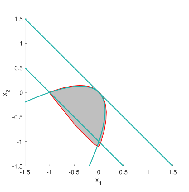
(a) Problem (19)

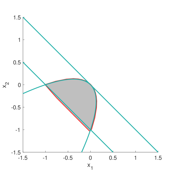
(b) Problem (20)

(c) Problem (21)

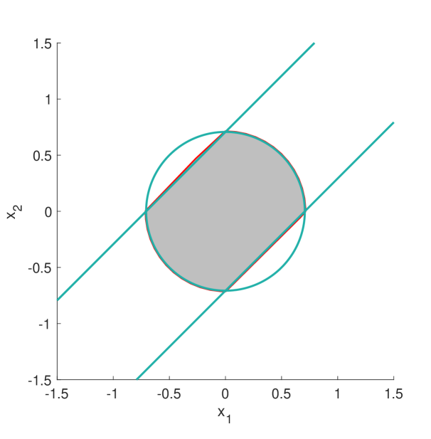
(d) Problem (22)

Figure 1. The feasible sets $\mathbf{K}$ (enclosed by the green curves) and their SDr approximations $\Lambda_{6}$ (the gray areas enclosed by the red curves) in Problem (19)-(22).

$k$		Problem (19)				Problem (20)
		$\mathscr{L}^{\star}_{k}(x)/\mathscr{L}^{\star}_{k}(1)$	$r^{\mbox{\tiny dual}}_{k}$	time		$\mathscr{L}^{\star}_{k}(x)/\mathscr{L}^{\star}_{k}(1)$	$r^{\mbox{\tiny dual}}_{k}$	time
$6$		$(-0.5368,-0.5964)$	$0.3775$	0.9s		$(-0.5158,-0.5364)$	$0.4494$	1.0s
$7$		$(-0.5280,-0.5780)$	$0.4009$	1.3s		$(-0.5121,-0.5289)$	$0.4600$	1.4s
$8$		$(-0.5220,-0.5644)$	$0.4182$	1.9s		$(-0.5096,-0.5235)$	$0.4676$	2.0s
9		$(-0.5178,-0.5541)$	0.4314	3.0s		$(-0.5078,-0.5195)$	0.4732	3.1s
10		$(-0.5147,-0.5461)$	0.4416	4.3s		$(-0.5065,-0.5164)$	0.4775	4.5s
11		$(-0.5123,-0.5397)$	0.4497	6.6s		$(-0.5054,-0.5140)$	0.4808	7.1s
12		$(-0.5105,-0.5346)$	0.4562	11.2s		$(-0.5046,-0.5121)$	0.4834	10.7s
13		$(-0.5092,-0.5306)$	0.4612	19.6s		$(-0.5041,-0.5106)$	0.4854	18.1s
14		$(-0.5090,-0.5297)$	0.4623	27.0s		$(-0.5037,-0.5095)$	0.4869	29.2s
15		$(-0.5082,-0.5277)$	0.4649	42.4s		$(-0.5036,-0.5089)$	0.4877	43.8s

Table 1. Computational results for Problem (19)-(20).

$k$		Problem (21)				Problem (22)
		$\mathscr{L}^{\star}_{k}(x)/\mathscr{L}^{\star}_{k}(1)$	$r^{\mbox{\tiny dual}}_{k}$	time		$\mathscr{L}^{\star}_{k}(x)/\mathscr{L}^{\star}_{k}(1)$	$r^{\mbox{\tiny dual}}_{k}$	time
$6$		$(0.7174,0.7174)$	$0.1597$	0.9s		$(-0.3633,0.3633)$	$0.8108$	67.3s
$7$		$(0.7152,0.7152)$	$0.1622$	1.3s		$(-0.3618,0.3618)$	$0.8148$	114s
$8$		$(0.7137,0.7137)$	$0.1640$	2.0s		$(-0.3606,0.3606)$	$0.8176$	171s
9		$(0.7125,0.7125)$	0.1653	2.9s		$(-0.3600,0.3600)$	0.8193	257s
10		$(0.7117,0.7117)$	0.1663	4.7s		$(-0.3596,0.3596)$	0.8203	328s
11		$(0.7110,0.7110)$	0.1671	7.1s		$(-0.3589,0.3589)$	0.8220	465s
12		$(0.7105,0.7105)$	0.1677	10.3s		$(-0.3584,0.3584)$	0.8232	640s
13		$(0.7100,0.7100)$	0.1682	17.3s		$(-0.3582,0.3582)$	0.8238	862s
14		$(0.7097,0.7097)$	0.1686	28.8s		$(-0.3579,0.3579)$	0.8246	1147s
15		$(0.7094,0.7094)$	0.1689	41.6s		$(-0.3576,0.3576)$	0.8255	1508s

Table 2. Computational results for Problem (21)-(22).

Remark 5.1.

From Table 1 and 2, we can see that our new SDP method for (FSIPP) behaves similarly to Lasserre’s measure-based SDP method for polynomial minimization problem [26]. That is, the sequence of lower bounds $\{r^{\mbox{\tiny dual}}_{k}\}_{k\in\mathbb{N}}$ increases rapidly in the first orders $k$, but rather slowly when close to $r^{\star}$. This behavior can also be expected from the convergence analysis discussed in Section 4. Nevertheless, the lower bounds obtained in a few orders indeed complement the upper bounds obtained by our previous work [15]. It is interesting to apply some acceleration techniques in [26, 29, 30] to improve the convergence rate of our new SDP method for (FSIPP). We leave it for our future investigation. ∎

The following example shows some computational behaviors of our SDP method compared with the discretization method by grids (see [19]) in computing lower bounds of $r^{\star}$.

Example 5.2.

Consider the problem

$$\left\{\begin{aligned} r^{\star}:=\min_{x\in{\mathbb{R}}^{n}}\ &\frac{\sum_{i=1}^{n}(x_{i}-1)^{4}}{\sum_{i=1}^{n}x_{i}+1}\\ \text{s.t.}\ &p(x,y)=\sum_{i=1}^{n}\left(1-\frac{(y_{i}-a_{i})^{2}}{4}\right)x_{i}^{2}-1\leq 0,\\ &\forall y\in\mathbf{Y}=[-1,1]^{n},\quad\varphi(x)=-\sum_{i=1}^{n}x_{i}\leq 0,\end{aligned}\right.$$ (23)

where each $a_{i}$ is a random number drawn from the standard uniform distribution on the interval $[-1,1]$. Obviously, the feasible set $\mathbf{K}$ is the intersection of the unit ball in ${\mathbb{R}}^{n}$ with the halfspace defined by $\sum_{i=1}^{n}x_{i}\geq 0$. Hence, the unique minimizer of (23) is $\left(\sqrt{\frac{1}{n}},\ldots,\sqrt{\frac{1}{n}}\right)$ and the optimal value is $n\left(\sqrt{\frac{1}{n}}-1\right)^{4}/(1+\sqrt{n})$. It is clear that A1-3 hold for (23).

Next, for each $n\in\mathbb{N}$, we generate random $a_{i}$’s in (23) and solve it by the SDP relaxation ($\mathrm{P}_{k}$) and the discretization method (10) with the regular grid (12) whose optimal value is denoted by $r_{N}^{\mbox{\tiny dis}}$. For the SDP relaxation ($\mathrm{P}_{k}$), we use the software Yalmip to implement it and call the SDP solver MOSEK to solve the resulting SDP problems. For the finitely constrained problem (10), as discussed at the end of Section 3.2, we have tried to solve it by (a) the bisection method for quasiconvex optimizaiton using the software CVXPY [10]; (b) the interior-point algorithm for nonlinear programming implemented in the Matlab command fmincon; (c) the SDP reformulation (11) which is implemented by Yalmip and solved by MOSEK. Our numerical experiments showed that the strategy (b) is more efficient and stable than the other two when $n$ is large, so we only report here the numerical results obtained by applying the Matlab command fmincon to (10). The initial feasible point for fmincon is set to be $0$.

We would like to test $n$ in (23) as large as possible for which we can gain meaningful lower bounds of $r^{\star}$ with these two methods. Therefore, we only compute and compare the first lower bound obtained by these methods, i.e., we let $k=1$ and $N=1$ in ($\mathrm{P}_{k}$) and (12), respectively. The computational results are shown in Table 3. As we can see, as $n$ increases, our SDP relaxations ($\mathrm{P}_{k}$) need much less time than the discretization method in obtaining alike lower bounds. ∎

$n$		$r^{\mbox{\tiny primal}}_{1}$/time		$r_{1}^{\mbox{\tiny dis}}$/time		$r^{\star}$
10		0.4414/3.7s		0.4752/0.9s		0.5252
11		0.5209/4.4s		0.5254/2.6s		0.6066
12		0.5959/5.4s		0.6042/8.1s		0.6882
13		0.6360/6.8s		0.7152/22s		0.7698
14		0.7438/9.5s		0.7565/1m13s		0.8511
15		0.8109/18s		0.8224/3m50s		0.9321
16		0.9050/23s		0.8815/12m40s		1.0125
17		0.9343/29s		0.9824/37m34s		1.0924
18		1.0070/45s		1.0835/2h13m		1.1716

Table 3. Computational results for Example 5.2.

Remark 5.2.

Remark that for the regular grids (12) in the discretization scheme, there are $(N+1)^{n}$ constaints to be generated from the grid points. The process could be very costly and the resulting problems become intractable for a large $n$. Of course, we are aware that there are other (commercial) softwares, which can deal with the process more efficiently and solve the resulting finitely constrained problems of much larger size. Meanwhile, the size of the semidefinite matrix in ($\mathrm{P}_{k}$) grows as $3\binom{m+\mathbf{d}}{m}+\binom{n+k}{n}$ and also becomes rapidly prohibitive as the order $k$ increases. Therefore, in view of the present status of available semidefinite solvers, we do not simply claim by Example 5.2 any computational superiority of our SDP relaxation method over the discretization scheme. Instead, we intend to illustrate by the encouraging results in Example 5.2 that our SDP relaxation method is promising to compute meaningful lower bounds of $r^{\star}$ with higher dimensional $\mathbf{Y}$ in a reasonable time. ∎

We end this paper with the following example to highlight the scalability of the alternatives ($\mathrm{P}^{\mbox{\tiny dsos}}_{k}$) and ($\mathrm{P}^{\mbox{\tiny sdsos}}_{k}$).

Example 5.3.

Consider the problem

$$\left\{\begin{aligned} r^{\star}:=\min_{x\in{\mathbb{R}}^{m}}\ &\sum_{i=1}^{m}(x_{i}-3)^{2}\\ \text{s.t.}\ &p(x,y)=\sum_{i=1}^{m}x_{i}^{d}-(1-y_{1}y_{2})\leq 0,\\ &\forall y\in\mathbf{Y}=\{y\in{\mathbb{R}}^{2}\mid y_{1}^{2}+y_{2}^{2}=1\},\end{aligned}\right.$$ (24)

where $d\in\mathbb{N}$ is even. Clearly, the feasible set $\mathbf{K}$ is $\{x\in{\mathbb{R}}^{m}\mid\sum_{i=1}^{m}x_{i}^{d}\leq 1/2\}$. Hence, the unique minimizer of (24) is $\left(\sqrt[d]{\frac{1}{2m}},\ldots,\sqrt[d]{\frac{1}{2m}}\right)$ and the optimal value is $m\left(\sqrt[d]{\frac{1}{2m}}-3\right)^{2}$. It is clear that A1-3 hold for (24).

Now we solve (24) using the relaxations ($\mathrm{P}^{\mbox{\tiny dsos}}_{k}$), ($\mathrm{P}^{\mbox{\tiny sdsos}}_{k}$) and ($\mathrm{P}_{k}$). For comparison, we implement all of the relaxations by means of the software package spotless_isos [2] which is written using the Systems Polynomial Optimization Toolbox [35], and solve the resulting problems by MOSEK. As we are interested in comparing the impacts of the dsos/sdsos/sos structures on the computation time and the obtained lower bound quality of the corresponding relaxations, we fix the order $k=1$ and let the numbers $(m,d)$ vary. The numerical results are reported in Table 4. Although the lower bounds $r^{\mbox{\tiny dsos}}_{1}$ and $r^{\mbox{\tiny sdsos}}_{1}$ are not as good as $r^{\mbox{\tiny primal}}_{1}$, the times for computing them are significantly less than that of $r^{\mbox{\tiny primal}}_{1}$. When $m$, $d$ are large and $r^{\mbox{\tiny primal}}_{1}$ is not available in a reasonable time, we can still get meaningful lower bounds $r^{\mbox{\tiny dsos}}_{1}$ and $r^{\mbox{\tiny sdsos}}_{1}$ by the alternatives ($\mathrm{P}^{\mbox{\tiny dsos}}_{k}$) and ($\mathrm{P}^{\mbox{\tiny sdsos}}_{k}$).

$(m,d)$		$r^{\mbox{\tiny dsos}}_{1}$/time		$r^{\mbox{\tiny sdsos}}_{1}$/time		$r^{\mbox{\tiny primal}}_{1}$/time		$r^{\star}$
(16, 4)		83.50/2.5s		102.79/3.3s		102.79/8.5s		106.46
(10, 6)		47.50/6.0s		55.25/9.6s		55.25/40s		57.26
(20, 4)		107.50/5.2s		131.07/6.8s		131.07/59s		135.44
(12, 6)		59.50/15s		67.41/24s		67.41/7m13s		69.76
(10, 8)		47.53/1m57s		51.83/2m39s		51.83/8h28m		53.47
(12, 8)		59.57/7m9s		63.09/10m45s		/>10h		65.02

Table 4. Computational results for Example 5.3.

Appendix A

We first recall some definitions and properties about the so-called needle polynomials required in the proof of Proposition 4.2.

Definition A.1.

For $k\in\mathbb{N}$, the Chebyshev polynomial $T_{k}(t)\in{\mathbb{R}}[t]_{k}$ is defined by

$$T_{k}(t)=\left\{\begin{aligned} &\cos(k\arccos t)&\text{for}\ |t|\leq 1,\\ &\frac{1}{2}(t+\sqrt{t^{2}-1})^{k}+\frac{1}{2}(t-\sqrt{t^{2}-1})^{k}&\text{for}\ |t|\geq 1.\end{aligned}\right.$$

Definition A.2.

[23] For $k\in\mathbb{N}$, $h\in(0,1)$, the needle polynomial $v_{k}^{h}(t)\in{\mathbb{R}}[t]_{4k}$ is defined by

$$v_{k}^{h}(t)=\frac{T_{k}^{2}(1+h^{2}-t^{2})}{T_{k}^{2}(1+h^{2})}.$$

Theorem A.1.

[8, 22, 23] For $k\in\mathbb{N}$, $h\in(0,1)$, the following properties hold for $v_{k}^{h}(t)$:

$$v_{k}^{h}(0)=1,$$

$$0\leq v_{k}^{h}(t)\leq 1 \text{for}\ t\in[-1,1],$$

$$v_{k}^{h}(t)\leq 4e^{-\frac{1}{2}kh} \text{for}\ t\in[-1,1]\ \text{with}\ |t|\geq h.$$

The following result gives a lower estimator which is used in the proof of Proposition 4.2 to lower bound the integral of the needle polynomial.

Proposition A.1.

[44, Lemma 13] Let $\phi(t)\in{\mathbb{R}}[t]_{k}$ be a polynomial of degree up to $k\in\mathbb{N}$, which is nonnegative over ${\mathbb{R}}_{\geq 0}$ and satisfies $\phi(0)=1,\phi(t)\leq 1$ for all $t\in[0,1]$. Let $\Phi_{k}:{\mathbb{R}}_{\geq 0}\rightarrow{\mathbb{R}}_{\geq 0}$ be defined by

$$\Phi_{k}(t)=\left\{\begin{aligned} &1-2k^{2}t&\text{if}\ t\leq\frac{1}{2k^{2}},\\ &0&\text{otherwise}.\end{aligned}\right.$$

Then $\Phi_{k}(t)\leq p(t)$ for all $t\in{\mathbb{R}}_{\geq 0}$.

Proof of Proposition 4.2 For any $k\in\mathbb{N}$, let $\rho(k)=\frac{1}{16k^{2}}$ and $h(k):=(4n+2)\log k/\lfloor k/2\rfloor$. Then, there exists a $k^{\prime}\in\mathbb{N}$ such that $\rho(k)\leq h(k)<\min\{\epsilon_{\mathbf{Y}},1\}$ for any $k\geq k^{\prime}$. Fix a $k\geq k^{\prime}$, a linear functional $\mathscr{L}_{k}\in({\mathbb{R}}[x]_{2\mathbf{d}})^{*}$ satisfying the conditions in (9), and a minimizer $y^{\star}$ of $\min_{y\in\mathbf{Y}}-\mathscr{L}_{k}(p(x,y))$. Using the needle polynomial $v_{k}^{h}(t)\in{\mathbb{R}}[t]$, define $\sigma_{k}(y):=v_{\lfloor k/2\rfloor}^{h(k)}(\|y-y^{\star}\|/(2\sqrt{n}))$. Then, the polynomial $\tilde{\sigma}:=\sigma_{k}/\int_{\mathbf{Y}}\sigma_{k}\mathrm{d}y\in\Sigma_{k}^{2}[y]$ and feasible to (15). Hence, by Taylor’s theorem,

$$E(\mathscr{L}_{k}) \leq\frac{1}{\int_{\mathbf{Y}}\sigma_{k}(y)\mathrm{d}y}\int_{\mathbf{Y}}-\mathscr{L}_{k}({p(x,y)})\sigma_{k}(y)\mathrm{d}y-p^{\star}_{k}$$ (25)

$$=\frac{1}{\int_{\mathbf{Y}}\sigma_{k}(y)\mathrm{d}y}\int_{\mathbf{Y}}\sigma_{k}(y)(-\mathscr{L}_{k}({p(x,y)}-p^{\star}_{k})\mathrm{d}y$$

$$\leq\frac{B_{1}}{\int_{\mathbf{Y}}\sigma_{k}(y)\mathrm{d}y}\int_{\mathbf{Y}}\sigma_{k}(y)\|y-y^{\star}\|\mathrm{d}y$$

Define two sets

$$\mathbf{Y}_{1}:=\mathbf{B}_{2\sqrt{n}h(k)}^{n}(y^{\star})\cap\mathbf{Y}\quad\text{and}\quad\mathbf{Y}_{2}:=\mathbf{B}_{2\sqrt{n}\rho(k)}^{n}(y^{\star})\cap\mathbf{Y}\subseteq\mathbf{Y}_{1}.$$

Then,

$$\int_{\mathbf{Y}}\sigma_{k}(y)\mathrm{d}y\geq\int_{\mathbf{Y}_{1}}\sigma_{k}(y)\mathrm{d}y\geq\int_{\mathbf{Y}_{2}}\sigma_{k}(y)\mathrm{d}y.$$ (26)

As $\mathbf{Y}\subseteq\mathbf{H}^{n}$,

$$\int_{\mathbf{Y}}\sigma_{k}(y)\|y-y^{\star}\|\mathrm{d}y =\int_{\mathbf{Y}_{1}}\sigma_{k}(y)\|y-y^{\star}\|\mathrm{d}y+\int_{\mathbf{Y}\setminus\mathbf{Y}_{1}}\sigma_{k}(y)\|y-y^{\star}\|\mathrm{d}y$$ (27)

$$\leq 2\sqrt{n}h(k)\int_{\mathbf{Y}_{1}}\sigma_{k}(y)\mathrm{d}y+2\sqrt{n}\int_{\mathbf{Y}\setminus\mathbf{Y}_{1}}\sigma_{k}(y)\mathrm{d}y.$$

By Theorem A.1, we have $\sigma_{k}(y)\leq 4e^{-\frac{1}{2}h(k)\lfloor k/2\rfloor}$ for any $y\in\mathbf{Y}\setminus\mathbf{Y}_{1}$ and hence

$$\int_{\mathbf{Y}\setminus\mathbf{Y}_{1}}\sigma_{k}(y)\mathrm{d}y\leq 4e^{-\frac{1}{2}h(k)\lfloor k/2\rfloor}\cdot\text{vol}(\mathbf{Y}\setminus\mathbf{Y}_{1})\leq 4e^{-\frac{1}{2}h(k)\lfloor k/2\rfloor}\cdot\text{vol}(\mathbf{H}^{n}).$$

Moreover, by Proposition A.1, we have

$$\sigma_{k}(y)\geq\Phi_{2k}(\|y-y^{\star}\|/2\sqrt{n})=1-8k^{2}(\|y-y^{\star}\|/2\sqrt{n})\geq\frac{1}{2},$$

for all $y\in\mathbf{Y}_{2}$. Therefore, A5 implies that

$$\int_{\mathbf{Y}_{2}}\sigma_{k}(y)\mathrm{d}y\geq\frac{1}{2}\text{vol}(\mathbf{Y}_{2})\geq\frac{1}{2}\eta_{\mathbf{Y}}2^{n}n^{n/2}\rho(k)^{n}\text{vol}(\mathbf{B}^{n})=\frac{\eta_{\mathbf{Y}}n^{n/2}\text{vol}(\mathbf{B}^{n})}{2^{3n+1}k^{2n}}.$$ (28)

Combining (25)-(28), we obtain

$$E(\mathscr{L}_{k}) \leq 2\sqrt{n}B_{1}\left(h(k)+4e^{-\frac{1}{2}h(k)\lfloor k/2\rfloor}\frac{2^{3n+1}k^{2n}\text{vol}(\mathbf{H}^{n})}{\eta_{\mathbf{Y}}n^{n/2}\text{vol}(\mathbf{B}^{n})}\right)$$ (29)

$$=2\sqrt{n}B_{1}(h(k)+Ce^{-\frac{1}{2}h(k)\lfloor k/2\rfloor}k^{2n})$$

The conclusion follows by substituting $h(k)=(4n+2)\log k/\lfloor k/2\rfloor$ in (29).∎

References

- [1] A. A. Ahmadi and A. Majumdar. DSOS and SDSOS optimization: LP and SOCP-based alternatives to sum of squares optimization. In 2014 48th Annual Conference on Information Sciences and Systems (CISS), pages 1–5, 2014.
- [2] A. A. Ahmadi and A. Majumdar. DSOS and SDSOS optimization: More tractable alternatives to sum of squares and semidefinite optimization. SIAM Journal on Applied Algebra and Geometry, 3(2):193–230, 2019.
- [3] A. A. Ahmadi, A. Olshevsky, P. A. Parrilo, and J. N. Tsitsiklis. NP-hardness of deciding convexity of quartic polynomials and related problems. Mathematical Programming, 137(1):453–476, 2013.
- [4] A. A. Ahmadi and P. A. Parrilo. A convex polynomial that is not sos-convex. Mathematical Programming, 135(1):275–292, 2012.
- [5] V. Baldoni, N. Berline, J. A. De Loera, B. Dutra, M. Köppe, S. Moreinis, G. Pinto, M. Vergne, and J. Wu. A User’s Guide for LattE integrale v1.7.2, 2013, software package LattE is available at http://www.math.ucdavis.edu/~latte/.
- [6] A. Ben-Tal and A. Nemirovski. Lectures on Modern Convex Optimization: Analysis, Algorithms, and Engineering Applications. MOS-SIAM Series on Optimization. Society for Industrial and Applied Mathematics, 2001.
- [7] M. J. Cánovas, D. Klatte, M. A. López, and J. Parra. Metric regularity in convex semi-infinite optimization under canonical perturbations. SIAM Journal on Optimization, 18(3):717–732, 2007.
- [8] E. de Klerk and M. Laurent. Worst-case examples for Lasserre’s measure-based hierarchy for polynomial optimization on the hypercube. Mathematics of Operations Research, 45(1):86–98, 2020.
- [9] E. de Klerk, M. Laurent, and Z. Sun. Convergence analysis for Lasserre’s measure-based hierarchy of upper bounds for polynomial optimization. Mathematical Programming, 162(1):363–392, 2017.
- [10] S. Diamond and S. Boyd. CVXPY: A Python-embedded modeling language for convex optimization. Journal of Machine Learning Research, 17(83):1–5, 2016.
- [11] G. B. Folland. How to integrate a polynomial over a sphere. The American Mathematical Monthly, 108(5):446–448, 2001.
- [12] M. A. Goberna and M. A. López. Recent contributions to linear semi-infinite optimization. 4OR, 15(3):221–264, 2017.
- [13] M. A. Goberna and M. A. López. Recent contributions to linear semi-infinite optimization: an update. Annals of Operations Research, 271(1):237–278, 2018.
- [14] J. Gouveia, P. Parrilo, and R. Thomas. Theta bodies for polynomial ideals. SIAM Journal on Optimization, 20(4):2097–2118, 2010.
- [15] F. Guo and L. Jiao. On solving a class of fractional semi-infinite polynomial programming problems. Computational Optimization and Applications, 80:439–481, 2021.
- [16] F. Guo and X. Sun. On semi-infinite systems of convex polynomial inequalities and polynomial optimization problems. Computational Optimization and Applications, 75(3):669–699, 2020.
- [17] J. Helton and J. Nie. Sufficient and necessary conditions for semidefinite representability of convex hulls and sets. SIAM Journal on Optimization, 20(2):759–791, 2009.
- [18] J. Helton and J. Nie. Semidefinite representation of convex sets. Mathematical Programming, 122(1):21–64, 2010.
- [19] R. Hettich and K. O. Kortanek. Semi-infinite programming: theory, methods, and applications. SIAM Review, 35(3):380–429, 1993.
- [20] C. Josz and D. Henrion. Strong duality in Lasserre’s hierarchy for polynomial optimization. Optimization Letters, 10(1):3–10, 2016.
- [21] Y. Y. K. Sekitani, J. Shi. General fractional programming: min-max convex-convex quadratic case. APORS-Development in Diversity and Harmony, pages 505–514, 1995.
- [22] A. Kroó. Multivariate “needle” polynomials with application to norming sets and cubature formulas. Acta Mathematica Hungarica, 147(1):46–72, 2015.
- [23] A. Kroó and J. J. Swetits. On density of interpolation points, a Kadec-type theorem, and Saff’s principle of contamination in -approximation. Constructive Approximation, 8(1):87–103, 1992.
- [24] J. B. Lasserre. Convex sets with semidefinite representation. Mathematical Programming, Ser. A, 120(2):457–477, 2009.
- [25] J. B. Lasserre. Convexity in semialgebraic geometry and polynomial optimization. SIAM Journal on Optimization, 19(4):1995–2014, 2009.
- [26] J. B. Lasserre. A new look at nonnegativity on closed sets and polynomial optimization. SIAM Journal on Optimization, 21(3):864–885, 2011.
- [27] J. B. Lasserre. An algorithm for semi-infinite polynomial optimization. TOP, 20(1):119–129, 2012.
- [28] J. B. Lasserre. Tractable approximations of sets defined with quantifiers. Mathematical Programming, 151(2):507–527, 2015.
- [29] J. B. Lasserre. Computing Gaussian & exponential measures of semi-algebraic sets. Advances in Applied Mathematics, 91:137–163, 2017.
- [30] J. B. Lasserre. Volume of sublevel sets of homogeneous polynomials. SIAM Journal on Applied Algebra and Geometry, 3(2):372–389, 2019.
- [31] J. Löfberg. YALMIP : a toolbox for modeling and optimization in MATLAB. In 2004 IEEE International Conference on Robotics and Automation (IEEE Cat. No.04CH37508), pages 284–289, 2004.
- [32] M. López and G. Still. Semi-infinite programming. European Journal of Operational Research, 180(2):491–518, 2007.
- [33] V. Magron, D. Henrion, and J. Lasserre. Semidefinite approximations of projections and polynomial images of semialgebraic sets. SIAM Journal on Optimization, 25(4):2143–2164, 2015.
- [34] A. Majumdar, A. A. Ahmadi, and R. Tedrake. Control and verification of high-dimensional systems with DSOS and SDSOS programming. In 53rd IEEE Conference on Decision and Control, pages 394–401, 2014.
- [35] A. Megretski. Systems Polynomial Optimization Tools (SPOT). https://github.com/spot-toolbox/spotless, 2010.
- [36] A. Mosek. The MOSEK Optimization Software. https://www.mosek.com/.
- [37] J. Nie. Semidefinite representability. In G. Blekherman, P. A. Parrilo, and R. R. Thomas, editors, Semidefinite Optimization and Convex Algebraic Geometry, MOS-SIAM Series on Optimization, chapter 6, pages 251–291. Society for Industrial and Applied Mathematics, Philadelphia, PA, 2012.
- [38] P. M. Pardalos and S. A. Vavasis. Quadratic programming with one negative eigenvalue is NP-hard. Journal of Global Optimization, 1(1):15–22, 1991.
- [39] J. Ponstein. Seven kinds of convexity. SIAM Review, 9(1):115–119, 1967.
- [40] M. Putinar. Positive polynomials on compact semi-algebraic sets. Indiana University Mathematics Journal, 42(3):969–984, 1993.
- [41] P. Rostalski. Bermeja - software for convex algebraic geometry. http://math.berkeley.edu/~philipp/cagwiki, 2010.
- [42] A. Shapiro. Semi-infinite programming, duality, discretization and optimality conditions. Optimzation, 58(2):133–161, 2009.
- [43] A. Shapiro and K. Scheinber. Duality, optimality conditions and perturbation analysis. In H. Wolkowicz, R. Saigal, and L. Vandenberghe, editors, Handbook of Semidefinite Programming - Theory, Algorithms, and Applications, pages 67–110. Kluwer Academic Publisher, Boston, 2000.
- [44] L. Slot and M. Laurent. Improved convergence analysis of Lasserre’s measure-based upper bounds for polynomial minimization on compact sets. Mathematical Programming, in press, 2020.
- [45] L. Wang and F. Guo. Semidefinite relaxations for semi-infinite polynomial programming. Computational Optimization and Applications, 58(1):133–159, 2013.
- [46] L. Wang, T. Ma, and Y. Xia. A linear-time algorithm for minimizing the ratio of quadratic functions with a quadratic constraint. Computational and Applied Mathematics, 40(4):150, 2021.
- [47] H. Wolkowicz, R. Saigal, and L. Vandenberghe. Handbook of Semidefinite Programming - Theory, Algorithms, and Applications. Kluwer Academic Publisher, Dordrecht, 2000.
- [48] Y. Xu, W. Sun, and L. Qi. On solving a class of linear semi-infinite programming by SDP method. Optimization, 64(3):603–616, 2015.
- [49] M. Yang and Y. Xia. On Lagrangian duality gap of quadratic fractional programming with a two-sided quadratic constraint. Optimization Letters, 14(3):569–578, 2020.