Legendre Expansions of Products of Functions with Applications to Nonlinear Partial Differential Equations

Rabia Djellouli, David Klein, Matthew Levy

1 Introduction

Fourier-type series have proven to be powerful tools for solving (semi-)analytically a large class of linear PDEs that arise in a range of applications, including wave propagation, heat diffusion, compressible and incompressible fluid mechanics, free surface flow, flow in porous media, particle flow, strength of materials, elasticity, structural dynamics, transport engineering, and electrical engineering. Fourier-type series have also been incorporated into a variety of numerical strategies for solving linear PDE formulation problems. For example, they have been used to construct absorbing boundary conditions (exact or approximate) to re-formulate exterior electromagnetic or acoustic scattering problems in bounded domains (see, for example, [1] and references therein). In addition, they have been extensively employed to generate exact solutions to serve as reference solutions for assessing the performance accuracy of numerical methods designed to solve PDEs (see, for example, [2]).

The use of Fourier-type series solution methods to solve linear PDEs have several attractive features. These include significant reduction of computational complexity, high accuracy levels, and cost-effectiveness. By contrast, for nonlinear problems, Fourier-type series have so far only been included in already established solution methodologies. Indeed, as is well-known [3], standard methods for solving nonlinear problems involve two-step approaches, where in the first step, the nonlinear problem under consideration is formulated as a set or sequence of linear problems via linearization processes such as gradient methods, fixed-point, or path following approaches. In the second step, the linear problems from the first step are solved using approximation methods employing various representations such as polynomial, Fourier-like expansions, spectral representation, wavelets, or reduced bases [4]. There is a second class of methods that uses approximation prior to the linearization process. The main difference between the two approaches is that this latter class of methods gives rise to a sequence of linear problems in finite dimensional vector spaces whereas the standard approaches involve infinite dimensional spaces (such as Sobolev spaces) prior to the application of the discretization schemes. We are not aware of any work in which Fourier-type expansions are employed as the primary tool for solving the nonlinear PDEs. The main obstacle is that the presence of the nonlinearity prevents a significant gain in terms of computational complexity.

In this paper, our focus is on Fourier-Legendre series [5, 6]. We prove new theorems on products of Fourier-Legendre series and show how they can be exploited to approximate solutions to a class of nonlinear PDEs in which the nonlinearity is a polynomial of degree 2. The method is generalizable to polynomials of arbitrary degree, and it is particularly well suited to PDEs with diffusion terms, since the diffusion operator is diagonal in the orthogonal basis of Legendre polynomials (in $L^{2}[-1,1]$).

More specifically, we show how the Fourier-Legendre coefficients of a product of two functions, $f$ and $g$, can be expressed in terms of the respective Fourier-Legendre coefficients of $f$ and $g$, and we derive an easily computable partial finite sum. The key ingredient is a well-known combinatorial formula that expresses the product of two Legendre polynomials as an explicit linear combination of Legendre polynomials [7, 8, 9, 10]. This is carried out in Section 2. Section 3 establishes upper bounds of rates of convergence for product series approximations, depending on the smoothness of the factors $f$ and of $g$. In Section 4, we illustrate how our results may be applied to find semi-analytic solutions to a class of nonlinear partial differential equations with diffusion, and quadratic polynomial nonlinearity. In Section 5, we summarize and assess our results, and identify further applications.

2 Product Theorem

Assume that $f,g,f\cdot g\in L^{2}([-1,1])$. Let $P_{n}(x)$ denote the $n$th Legendre Polynomial [6], and denote the expansions of $f$ and $g$ in the orthogonal basis $\{P_{n}(x)\}$ by,

$$f(x)=\sum_{n=0}^{\infty}\alpha_{n}P_{n}(x)\qquad g(x)=\sum_{m=0}^{\infty}\beta_{n}P_{m}(x)$$ (2.1)

where [6],

$$\alpha_{n}=\frac{2n+1}{2}\int_{-1}^{1}f(x)P_{n}(x)dx,\qquad\beta_{m}=\frac{2m+1}{2}\int_{-1}^{1}g(x)P_{m}(x)dx.$$ (2.2)

Since the function $f\cdot g\in L^{2}([-1,1])$, it also has a Fourier-Legendre expansion,

$$(f\cdot g)(x)=\sum_{k=0}^{\infty}\mu_{k}P_{k}(x).$$ (2.3)

Assuming pointwise and absolute convergence of Eqs (2.1), we show in this section how to express each coefficient $\mu_{k}$ as a function of the coefficients $\{\alpha_{n}\}_{n\in\{0,1,2,\dots\}}$ and $\left\{\beta_{m}\right\}_{m\in\{0,1,2,\dots\}}$ in the form of an infinite series, by first finding finite sum approximations.

Unless otherwise indicated, we assume throughout that the series in Eqs.(2.1) converge in the sense of $L^{2}([-1,1])$ and with pointwise absolute convergence. This is the case, for example, when $f$ and $g$ are absolutely continuous on $[-1,1]$ and $f^{\prime}$ and $g^{\prime}$ are of bounded variation, conditions that hold for the case that $f$ and $g$ are continuously differentiable [13]. Under these assumptions, we can express the product of the two series in Eq.(2.1) as a sum of products of Legendre polynomials as follows,

$$(f\cdot g)(x)=\left(\sum_{n=0}^{\infty}\alpha_{n}P_{n}(x)\right)\left(\sum_{m=0}^{\infty}\beta_{n}P_{m}(x)\right)=\sum_{n=0}^{\infty}\sum_{\ell=0}^{n}\alpha_{n-\ell}\beta_{\ell}P_{n-\ell}(x)P_{\ell}(x)$$ (2.4)

Let $N$ be a positive integer. We define the following two convenient sequences:

$$\alpha_{n}^{N}=\begin{cases}\alpha_{n}&\text{if}\,\,n\leqslant N\\ 0&\text{otherwise}\end{cases}\qquad\qquad\beta_{n}^{N}=\begin{cases}\beta_{n}&\text{if}\,\,n\leqslant N\\ 0&\text{otherwise}\end{cases}$$ (2.5)

Substituting $\alpha_{n}^{N}$ and $\beta_{n}^{N}$ for $\alpha_{n}$ and $\beta_{n}$ respectively in Eq.(2.4) gives,

$$\left(\sum_{n=0}^{N}\alpha_{n}P_{n}(x)\right)\left(\sum_{m=0}^{N}\beta_{n}P_{m}(x)\right) =\left(\sum_{n=0}^{\infty}\alpha_{n}^{N}P_{n}(x)\right)\left(\sum_{m=0}^{\infty}\beta_{n}^{N}P_{m}(x)\right)$$ (2.6)

$$=\sum_{n=0}^{\infty}\sum_{\ell=0}^{n}\alpha_{n-\ell}^{N}\beta_{\ell}^{N}P_{n-\ell}(x)P_{\ell}(x)$$ (2.7)

$$=\sum_{n=0}^{2N}\sum_{\ell=0}^{n}\alpha_{n-\ell}^{N}\beta_{\ell}^{N}P_{n-\ell}(x)P_{\ell}(x),$$ (2.8)

where the last step follows because all terms in Eq.(2.7) with $n>2N$ are zero.

In addition, assuming that both series in Eqs.(2.1) converge uniformly and that $f$ or $g$ is bounded on $[-1,1]$ we have,

$$(f\cdot g)(x) =\lim_{N\to\infty}\left[\left(\sum_{n=0}^{N}\alpha_{n}P_{n}(x)\right)\left(\sum_{m=0}^{N}\beta_{n}P_{m}(x)\right)\right]$$ (2.9)

$$=\lim_{N\to\infty}\sum_{n=0}^{2N}\sum_{\ell=0}^{n}\alpha_{n-\ell}^{N}\beta_{\ell}^{N}P_{n-\ell}(x)P_{\ell}(x)$$ (2.10)

and the convergence is uniform.

To proceed further, we use the fact that the product of any two Legendre polynomials can be expressed as a linear combination of Legendre polynomials according to this formula (see for example [10]),

$$\begin{split}P_{m}(x)P_{n}(x)&=\\ \sum_{j=0}^{\min(m,n)}&\frac{\left(\frac{1}{2}\right)_{j}\left(\frac{1}{2}\right)_{m-j}\left(\frac{1}{2}\right)_{n-j}(m+n-j)!}{j!(m-j)!(n-j)!\left(\frac{3}{2}\right)_{m+n-j}}\left(2(m+n-2j)+1\right)P_{m+n-2j}(x),\end{split}$$ (2.11)

where $(a)_{r}$ is the rising factorial function given by,

$$(a)_{0}=1,\qquad(a)_{r}=a(a+1)(a+2)\dots(a+(r-1)),\qquad r=1,2,3,\dots$$

Thus,

$$\sum_{\ell=0}^{k}\alpha_{k-\ell}\beta_{\ell}P_{k-\ell}(x)P_{\ell}(x)$$

$$=\sum_{\ell=0}^{k}\alpha_{k-\ell}\beta_{\ell}\left[\sum_{j=0}^{\min(k-\ell,\ell)}\frac{\left(\frac{1}{2}\right)_{j}\left(\frac{1}{2}\right)_{k-\ell-j}\left(\frac{1}{2}\right)_{\ell-j}(k-j)!}{j!(k-\ell-j)!(\ell-j)!\left(\frac{3}{2}\right)_{k-j}}\left(2(k-2j)+1)\right)P_{k-2j}(x)\right].$$ (2.12)

For simplicity of notation, define $A_{jk\ell}$ by,

$$A_{jk\ell}=\frac{\left(\frac{1}{2}\right)_{j}\left(\frac{1}{2}\right)_{k-\ell-j}\left(\frac{1}{2}\right)_{\ell-j}(k-j)!}{j!(k-\ell-j)!(\ell-j)!\left(\frac{3}{2}\right)_{k-j}}\left(2(k-2j)+1\right),$$ (2.13)

so that,

$$\sum_{\ell=0}^{k}\alpha_{k-\ell}\beta_{\ell}P_{k-\ell}(x)P_{\ell}(x)=\sum_{\ell=0}^{k}\sum_{j=0}^{\min(k-\ell,\ell)}\alpha_{k-\ell}\beta_{\ell}A_{jk\ell}P_{k-2j}(x),$$ (2.14)

with an analogous equation holding when $\alpha_{n}^{N}$ and $\beta_{n}^{N}$ are substituted for $\alpha_{n}$ and $\beta_{n}$ respectively.

Remark 1.

$A_{jk\ell}$ is undefined unless $j\leq\min(k-\ell,\ell)$ because of the terms $(k-\ell-j)!$ and $(\ell-j)!$ in the denominator of Eq.(2.13).

Lemma 1.

For any integers $j,k,\ell$ satisfying $0\leq j\leq\min(k-\ell,\ell)\leq\ell\leq k$,

$$0<A_{jk\ell}\leq 1,$$

where $A_{jk\ell}$ is given by Eq.(2.13).

Proof.

Set $x=1$ so that $P_{n}(x)=1$ for all $n=0,1,2\dots$, in Eq.(2.14). Now choose any $k_{0}$ and any $\ell_{0}\leq k_{0}$. Choose functions $f$ and $g$ so that $\beta_{\ell}=1$ if $\ell=\ell_{0}$ and $\beta_{\ell}=0$ otherwise, and so that $\alpha_{n}=1$ for $n=0,1,\dots,k_{0}$. Then Eq.(2.14) becomes,

$$1=\sum_{j=0}^{\min(k_{0}-\ell_{0},\ell_{0})}A_{jk_{0}\ell_{0}}$$ (2.15)

Since each summand in Eq.(2.15) is positive, it follows that each is bounded by $1$. ∎

Next, we combine Eqs(2.4), (2) and (2.13) to deduce that,

$$(f\cdot g)(x)=\sum_{k=0}^{\infty}\sum_{\ell=0}^{k}\sum_{j=0}^{\min(k-\ell,\ell)}\alpha_{k-\ell}\beta_{\ell}A_{jk\ell}P_{k-2j}(x),$$ (2.16)

and similarly using Eq.(2.9), we obtain,

$$(f\cdot g)(x)=\lim_{N\to\infty}\sum_{k=0}^{2N}\sum_{\ell=0}^{k}\sum_{j=0}^{\min(k-\ell,\ell)}\alpha_{k-\ell}^{N}\beta_{\ell}^{N}A_{jk\ell}P_{k-2j}(x).$$ (2.17)

Again, under the assumption that the series in Eq.(2.1) converge uniformly and that $f$ or $g$ is bounded on $[-1,1]$, the convergence in Eq.(2.16) is uniform.

The next lemma enables us to make a change of dummy variables and then interchange the inner two sums in Eqs. (2.16) and (2.17).

Lemma 2.

For nonnegative integers $j,k,\ell$,

$$\chi_{[0\leq\ell\leq k]}\cdot\chi_{[0\leq j\leq\min(k-\ell,\ell)]}=\chi_{[j\leq\ell\leq k-j]}\cdot\chi_{[0\leq j\leq\frac{k}{2}]}$$

Proof.

Observe first that $\chi_{[0\leq j\leq\min(k-\ell,\ell)]}=\chi_{[0\leq j\leq\ell]}\cdot\chi_{[0\leq j\leq k-\ell]}$. Thus, it suffices to show that

$$\chi_{[0\leq\ell\leq k]}\cdot\chi_{[0\leq j\leq k-\ell]}\cdot\chi_{[0\leq j\leq\ell]}=\chi_{[j\leq\ell\leq k-j]}\cdot\chi_{[0\leq j\leq\frac{k}{2}]}$$ (2.18)

We show that left side of Eq.(2.18) $=1$ if and only if the right side $=1$.

Assume that the left side equals 1. Then $0\leq j\leq k-\ell$ and $j\leq\ell$. Adding these inequalities, it follows that $0\leq 2j\leq k$ and therefore $0\leq j\leq\frac{k}{2}$. If the left side equals 1, it also follows that $j\leq\ell$ and $0\leq j\leq k-\ell$. Therefore $0\leq\ell\leq k-j$. Thus, the right side of the equation $=1$.

Next, assume that the right side of Eq.(2.18) equals 1. Then, $0\leq j\leq\frac{k}{2}$ and $j\leq\ell\leq k-j$. It follows that $0\leq j\leq\ell$ and $0\leq j\leq k-\ell$ and thus $\chi_{[0\leq\ell\leq k]}\cdot\chi_{[0\leq j\leq k-\ell]}=1$. Also, since $\ell\leq k-j$, then $\ell\leq k$ and $\chi_{[0\leq j\leq\ell]}=1$ and the right side of Eq.(2.18) equals 1. ∎

Corollary 1.

Let $f$ and $g$ be given as in Eqs. (2.1) with pointwise absolute convergence. Then, for each $x\in[-1,1]$, we have,

$$(f\cdot g)(x)=\lim_{N\to\infty}\sum_{k=0}^{N}\sum_{j=0}^{\lfloor\frac{k}{2}\rfloor}\sum_{\ell=j}^{k-j}\alpha_{k-\ell}\beta_{\ell}A_{jk\ell}P_{k-2j}(x),$$ (2.19)

where $\lfloor\frac{k}{2}\rfloor$ is the greatest integer less than or equal to $k/2$. If both series in Eq.(2.1) converge uniformly and $f$ or $g$ is bounded on $[-1,1]$, then,

$$(f\cdot g)(x)=\lim_{N\to\infty}\sum_{k=0}^{2N}\sum_{j=0}^{\lfloor\frac{k}{2}\rfloor}\sum_{\ell=j}^{k-j}\alpha_{k-\ell}^{N}\beta_{\ell}^{N}A_{jk\ell}P_{k-2j}(x),$$ (2.20)

with uniform convergence.

Proof.

From Lemma 2, we have for any $k\geq 0$,

$$\sum_{\ell=0}^{k}\sum_{j=0}^{\min(k-\ell,\ell)}\alpha_{k-\ell} \beta_{\ell}A_{jk\ell}P_{k-2j}(x)$$

$$=\sum_{\ell=0}^{\infty}\sum_{j=0}^{\infty}\chi_{[0\leq\ell\leq k]} \cdot\chi_{[0\leq j\leq\min(k-\ell,\ell)]}\alpha_{k-\ell}\beta_{\ell}A_{jk\ell}P_{k-2j}(x)$$

$$=\sum_{j=0}^{\infty}\sum_{\ell=0}^{\infty}\chi_{[j\leq\ell\leq k-j]}\chi_{[0\leq j\leq\lfloor\frac{k}{2}\rfloor]}\alpha_{k-\ell}\beta_{\ell}A_{jk\ell}P_{k-2j}(x)$$

$$=\sum_{j=0}^{\lfloor\frac{k}{2}\rfloor}\sum_{\ell=j}^{k-j}\alpha_{k-\ell}\beta_{\ell}A_{jk\ell}P_{k-2j}(x).$$ (2.21)

Combining with Eq.(2.16) gives,

$$(f\cdot g)(x)=\sum_{k=0}^{\infty}\sum_{j=0}^{\lfloor\frac{k}{2}\rfloor}\sum_{\ell=j}^{k-j}\alpha_{k-\ell}\beta_{\ell}A_{jk\ell}P_{k-2j}(x)$$

with pointwise convergence. Uniform convergence of Eq.(2.20) follows from the uniform convergence of Eq.(2.17). ∎

Theorem 1.

Let $f$ and $g$ be given as in Eqs. (2.1). Then,

(a) For each $N=0,1,2\dots$,

$$\sum_{k=0}^{N}\sum_{\ell=0}^{k}\sum_{j=0}^{\min(k-\ell,\ell)}\alpha_{k-\ell} \beta_{\ell}A_{jk\ell}P_{k-2j}(x)$$ (2.22)

$$= \sum_{n=0}^{N}\left[\sum_{m=0}^{\lfloor\frac{N-n}{2}\rfloor}\sum_{\ell=m}^{n+m}\alpha_{n+2m-\ell}\beta_{\ell}A_{m,n+2m,\ell}\right]P_{n}(x)$$

(b) Assuming pointwise absolute convergence in Eqs. (2.1),

$$(f\cdot g)(x)=\lim_{N\to\infty}\sum_{n=0}^{N}\left[\sum_{m=0}^{\lfloor\frac{N-n}{2}\rfloor}\sum_{\ell=m}^{n+m}\alpha_{n+2m-\ell}\beta_{\ell}A_{m,n+2m,\ell}\right]P_{n}(x),$$ (2.23)

for each $x\in[-1,1]$.

(c) If the series in Eq.(2.1) converge uniformly and $f$ or $g$ is bounded on $[-1,1]$, then,

$$(f\cdot g)(x)=\lim_{N\to\infty}\sum_{n=0}^{2N}\left[\sum_{m=0}^{\lfloor\frac{2N-n}{2}\rfloor}\sum_{\ell=m}^{n+m}\alpha_{n+2m-\ell}^{N}\beta_{\ell}^{N}A_{m,n+2m,\ell}\right]P_{n}(x),$$ (2.24)

and the convergence is uniform.

Proof.

For Part (a), observe from the proof of Corollary 1 that for each $N$,

$$\sum_{k=0}^{N}\sum_{\ell=0}^{k}\sum_{j=0}^{\min(k-\ell,\ell)}\alpha_{k-\ell}\beta_{\ell}A_{jk\ell}P_{k-2j}(x)=\sum_{k=0}^{N}\sum_{j=0}^{\lfloor\frac{k}{2}\rfloor}\sum_{\ell=j}^{k-j}\alpha_{k-\ell}\beta_{\ell}A_{jk\ell}P_{k-2j}(x).$$ (2.25)

In order to make a change of variables for the first two sums, $\sum\limits_{k=0}^{N}\sum\limits_{j=0}^{\lfloor\frac{k}{2}\rfloor}$, on the right side of Eq. (2.25), we define a linear transformation $T:\mathbb{R}^{2}\to\mathbb{R}^{2}$ by

$$(n,m)=T(k,j)=(k-2j,j).$$ (2.26)

Note that, in this expression the variables $j,k,n,m$ are real numbers, but below we will restrict them to take integer values. Since $T$ is a linear homeomorphism, it maps line segments to line segments and boundaries and interiors respectively of closed sets to boundaries and interiors respectively of closed sets, in the plane.

The the first two sums $\sum\limits_{k=0}^{N}\sum\limits_{j=0}^{\lfloor\frac{k}{2}\rfloor}$ on the right side of Eq. (2.25) can be expressed as a finite sum of the points $(k,j)$ in the triangular region in $\mathbb{R}^{2}\cap\mathbb{Z}^{2}$ whose boundary in $\mathbb{R}^{2}$ is the triangle consisting of the union of the following three line segments:

$$\{(k,0)\mid 0\leq k\leq N\},\quad\left\{(k,j)\mathrel{}\middle|\mathrel{}0\leq k\leq N,j=\frac{k}{2}\right\},\quad\left\{(N,j)\mathrel{}\middle|\mathrel{}0\leq j\leq\frac{N}{2}\right\}.$$

Under the transformation $T$ of (2.26), the above triangular region is mapped to the region whose boundary is the triangle consisting of the union of the following line segments:

$$\{(n,0)\mid 0\leq n\leq N\},\,\left\{(0,m)\mathrel{}\middle|\mathrel{}0\leq m\leq\frac{N}{2}\right\},\,\left\{(n,m)\mathrel{}\middle|\mathrel{}0\leq n\leq N,m=\frac{N-n}{2}\right\}.$$

Therefore, with the change of variables, $n=k-2j$ and $m=j$, we can make the substitutions,

$$k=n+2j=n+2m,\qquad k-j=n+j=n+m,$$

and find that,

$$\sum_{k=0}^{N}\sum_{j=0}^{\lfloor\frac{k}{2}\rfloor}\sum_{\ell=j}^{k-j}\alpha_{k-\ell} \beta_{\ell}A_{jk\ell}P_{k-2j}(x)$$ (2.27)

$$= \sum_{n=0}^{N}\left[\sum_{m=0}^{\lfloor\frac{N-n}{2}\rfloor}\sum_{\ell=m}^{n+m}\alpha_{n+2m-\ell}\beta_{\ell}A_{m,n+2m,\ell}\right]P_{n}(x),$$

thus establishing Part (a). Parts (b) and (c) now follow from part (a) and Corollary 1.
∎

In Lemma 3 below, and elsewhere in our paper, we make use of this result from Wang [11]:

Theorem 2.

(Wang [11]) Suppose that $f,f^{\prime},\dots,f^{(j-1)}$ are absolutely continuous on $[-1,1]$ and $f^{(j)}$ has bounded variation. Then, using the notation of Eq.(2.1), for $n\geq j+1$ and $j\geq 1$,

$$|\alpha_{n}|\leq\frac{\sqrt{2/\pi}||f^{(j)}||}{\sqrt{n-\frac{2j+1}{2}}\,(n-\frac{1}{2})(n-\frac{3}{2})\cdots(n-\frac{2j-1}{2})},$$ (2.28)

where it is assumed that

$$||f^{(j)}||\equiv\int_{-1}^{1}\frac{|f^{(j+1)}(x)|}{(1-x^{2})^{1/4}}dx<\infty.$$ (2.29)

If $j=0$, then $|\alpha_{n}|\leq\sqrt{2/\pi}||f||/\sqrt{n-\frac{1}{2}}$ for $n\geq 1$.

Remark 2.

It is a well-known result from measure theory that a function of bounded variation on a closed interval is differentiable almost everywhere with respect to Lebesgue measure [12]. It follows that Eq.(2.29) is meaningful.

Lemma 3.

Let $n$ and $j$ be positive integers. If $n\geq j+1$, then

$$\sqrt{n-\frac{2j+1}{2}}\left(n-\frac{1}{2}\right)\left(n-\frac{3}{2}\right)\cdots\left(n-\frac{2j-1}{2}\right)\geq(n-j)^{\frac{2j+1}{2}}$$ (2.30)

Proof.

The proof is by induction on $j$. If $j=1$ and $n\geq 2$, then

$$\sqrt{n-\frac{3}{2}}\left(n-\frac{1}{2}\right)\geq(n-1)^{3/2}$$ (2.31)

is easily verified. Next, assume that the result holds for $j=j_{0}$, and let $n^{\prime}=n-1$. Then,

$$\sqrt{n-\frac{2j_{0}+3}{2}}\left(n-\frac{1}{2}\right)\left(n-\frac{3}{2}\right)\cdots\left(n-\frac{2j_{0}+1}{2}\right)\\ =\sqrt{n-1-\frac{2j_{0}+1}{2}}\left(n-1+\frac{1}{2}\right)\left(n-1-\frac{1}{2}\right)\cdots\left(n-1-\frac{2j_{0}-1}{2}\right)\\ =\left(n^{\prime}+\frac{1}{2}\right)\sqrt{n^{\prime}-\frac{2j_{0}+1}{2}}\left(n^{\prime}-\frac{1}{2}\right)\cdots\left(n^{\prime}-\frac{2j_{0}-1}{2}\right)\\ \geq\left(n^{\prime}+\frac{1}{2}\right)(n^{\prime}-j_{0})^{\frac{2j_{0}+1}{2}}\geq(n^{\prime}-j_{0})^{\frac{2j_{0}+3}{2}}\qquad\qquad\qquad\qquad$$ (2.32)

for $n^{\prime}\geq j_{0}+1$, where the first inequality in the last line follows by induction. Thus, for $n\geq(j_{0}+1)+1$,

$$\sqrt{n-\frac{2(j_{0}+1)+1}{2}}\left(n-\frac{1}{2}\right)\left(n-\frac{3}{2}\right)\cdots\left(n-\frac{2(j_{0}+1)-1}{2}\right)\\ \geq(n-(j_{0}+1))^{\frac{2(j_{0}+1)+1}{2}},\qquad$$ (2.33)

and the induction argument is complete. ∎

The following consequence of Theorem 2 and Lemma 3 is now immediate.

Corollary 2.

Suppose that $f,f^{\prime},\dots,f^{(j-1)}$ are absolutely continuous on $[-1,1]$ and $f^{(j)}$ has bounded variation. Then, using the notation of Eq.(2.1), for $n\geq j+1$ and $j\geq 1$,

$$|\alpha_{n}|\leq\frac{\sqrt{2/\pi}||f^{(j)}||}{\sqrt{n-\frac{2j+1}{2}}\,(n-\frac{1}{2})(n-\frac{3}{2})\cdots(n-\frac{2j-1}{2})}\leq\frac{\sqrt{2/\pi}||f^{(j)}||}{\left(n-j\right)^{(2j+1)/2}}$$ (2.34)

Lemma 4.

Suppose that $f$ and $g$ are absolutely continuous on $[-1,1]$ and $f^{\prime}$ and $g^{\prime}$ are of bounded variation. Then, the collection

$$\left\{\sum_{n=0}^{N}\left[\sum_{m=0}^{\lfloor\frac{N-n}{2}\rfloor}\sum_{\ell=m}^{n+m}\alpha_{n+2m-\ell}\beta_{\ell}A_{m,n+2m,\ell}\right]P_{n}(x)\right\}$$

is uniformly bounded in $N$ and $x$.

Proof.

From Eqs.(2.14) and (2.22), we have,

$$\sum_{n=0}^{N}\left[\sum_{m=0}^{\lfloor\frac{N-n}{2}\rfloor}\sum_{\ell=m}^{n+m}\alpha_{n+2m-\ell}\beta_{\ell}A_{m,n+2m,\ell}\right] P_{n}(x)$$

$$=\sum_{n=0}^{N}\sum_{\ell=0}^{n}\sum_{j=0}^{\min(n-\ell,\ell)}\alpha_{n-\ell}\beta_{\ell}A_{jn\ell} P_{n-2j}(x)$$ (2.35)

$$=\sum_{n=0}^{N}\sum_{\ell=0}^{n}\alpha_{n-\ell}\beta_{\ell}P_{n-\ell}(x) P_{\ell}(x)$$

Thus, it suffices to show that the collection,

$$\left\{\sum_{n=0}^{N}\sum_{\ell=0}^{n}|\alpha_{n-\ell}\beta_{\ell}P_{n-\ell}(x)P_{\ell}(x)|\right\}$$

is uniformly bounded in $N$ and in $x$. Since $|P_{n}(x)|\leq 1$ for all $n$ and $x\in[-1,1]$, we show that the set of numbers,

$$\left\{\sum_{n=0}^{N}\sum_{\ell=0}^{n}|\alpha_{n-\ell}\beta_{\ell}|\right\}$$

is uniformly bounded in $N$. Using Corollary 2 with $j=1$, we have the following bounds,

$$|\alpha_{n}| \leq\frac{A_{1}}{\sqrt{n-\frac{3}{2}}\left(n-\frac{1}{2}\right)}\leq\frac{A_{1}}{\left(n-1\right)^{3/2}}$$ (2.36)

$$|\beta_{n}| \leq\frac{B_{1}}{\sqrt{n-\frac{3}{2}}\left(n-\frac{1}{2}\right)}\leq\frac{B_{1}}{\left(n-1\right)^{3/2}},$$ (2.37)

for $n\geq 2$, where $A_{1}$ and $B_{1}$ are constants depending on $f$ and $g$ respectively. For $n\geq 6$ we may write,

$$\sum_{\ell=0}^{n}|\alpha_{n-\ell}\beta_{\ell}|=\sum_{\ell=0}^{2}|\alpha_{n-\ell}\beta_{\ell}|+\sum_{\ell=0}^{2}|\beta_{n-\ell}\alpha_{\ell}|+\sum_{\ell=3}^{n-3}|\alpha_{n-\ell}\beta_{\ell}|\\$$ (2.38)

and the sum on $n$ of the first two terms on the right side of Eq.(2.38) is finite by Eqs.(2.36) and (2.37). Again, by Eqs.(2.36) and (2.37), the third term on the right side of Eq.(2.38) is bounded as follows,

$$\sum_{\ell=3}^{n-3}|\alpha_{n-\ell}\beta_{\ell}| \leq A_{1}B_{1}\sum_{\ell=3}^{n-3}\frac{1}{\left(n-\ell-1\right)^{3/2}\left(\ell-1\right)^{3/2}}$$ (2.39)

$$<A_{1}B_{1}\int_{2}^{n-2}\frac{dx}{(n-x-1)^{3/2}(x-1)^{3/2}}$$ (2.40)

$$=A_{1}B_{1}\frac{4(n-4)}{\sqrt{n-3}(n-2)^{2}},$$ (2.41)

which is summable on $n$. The integral in Eq.(2.40) is an upper bound for the sum in Eq.(2.39) because the integrand is a convex function with minimum at $n/2$. Thus, the set

$$\left\{\sum_{n=0}^{N}\sum_{\ell=0}^{n}|\alpha_{n-\ell}\beta_{\ell}|\right\}$$ (2.42)

is uniformly bounded in $N$, and the lemma is proved. ∎

Theorem 3.

Suppose that $f$ and $g$ are absolutely continuous on $[-1,1]$ and $f^{\prime}$ and $g^{\prime}$ are of bounded variation. Then, the Fourier-Legendre expansion of $f\cdot g$ in $L^{2}([-1,1])$ is given by,

$$(f\cdot g)(x)=\sum_{n=0}^{\infty}\left[\sum_{m=0}^{\infty}\sum_{\ell=m}^{n+m}\alpha_{n+2m-\ell}\beta_{\ell}A_{m,n+2m,\ell}\right]P_{n}(x).$$ (2.43)

Thus, in the notation of Eq.(2.3),

$$\mu_{k}=\sum_{m=0}^{\infty}\sum_{\ell=m}^{k+m}\alpha_{k+2m-\ell}\beta_{\ell}A_{m,k+2m,\ell}.$$ (2.44)

Proof.

We first note that the inner product on $L^{2}([-1,1])$ given by,

$$\langle\phi,\psi\rangle=\int_{-1}^{1}\phi(x)\psi(x)\,dx$$ (2.45)

is continuous in the $L^{2}([-1,1])$ Hilbert space topology. To simplify the notation, we set

$$\phi_{N}(x)=\sum_{n=0}^{N}\left[\sum_{m=0}^{\lfloor\frac{N-n}{2}\rfloor}\sum_{\ell=m}^{n+m}\alpha_{n+2m-\ell}\beta_{\ell}A_{m,n+2m,\ell}\right]P_{n}(x).$$ (2.46)

By Theorem 1b, $(f\cdot g)(x)=\lim_{N\to\infty}\phi_{N}(x)$ pointwise, and by Lemma 4 the sequence$\{\phi_{N}(x)\}$ is uniformly bounded by a constant on $[-1,1]$. Thus, by the Dominated Convergence Theorem $(f\cdot g)(x)=\lim_{N\to\infty}\phi_{N}(x)$ in $L^{2}([-1,1])$. Then, referring to Eq.(2.3), we find that,

$$\frac{2}{2k+1}\mu_{k}= \,\langle f\cdot g,P_{k}\rangle$$ (2.47)

$$= \,\langle\lim_{N\to\infty}\phi_{N},P_{k}\rangle$$ (2.48)

$$= \,\lim_{N\to\infty}\langle\phi_{N},P_{k}\rangle$$ (2.49)

$$= \,\frac{2}{2k+1}\lim_{N\to\infty}\sum_{m=0}^{\lfloor\frac{N-k}{2}\rfloor}\sum_{\ell=m}^{k+m}\alpha_{k+2m-\ell}\beta_{\ell}A_{m,k+2m,\ell},$$ (2.50)

where the last step follows from orthogonality of the Legendre Polynomials. Thus,

$$\mu_{k}= \lim_{N\to\infty}\sum_{m=0}^{\lfloor\frac{N-k}{2}\rfloor}\sum_{\ell=m}^{k+m}\alpha_{k+2m-\ell}\beta_{\ell}A_{m,k+2m,\ell}$$ (2.51)

$$= \sum_{m=0}^{\infty}\sum_{\ell=m}^{k+m}\alpha_{k+2m-\ell}\beta_{\ell}A_{m,k+2m,\ell}.$$ (2.52)

∎

3 Rates of Convergence

In this section, we collect results on the rate of convergence of the Fourier-Legendre series for $f\cdot g$ and for the rates of convergence of the series in Eq. (2.44) for the coefficients $\{\mu_{k}\}$. For the sake of notational simplicity, we adopt the following conventions.

$$A_{j}= \sqrt{2/\pi}||f^{(j)}||$$ (3.1)

$$B_{j}= \sqrt{2/\pi}||g^{(j)}||$$ (3.2)

$$C_{j}= \sqrt{2/\pi}||(fg)^{(j)}||$$ (3.3)

for $j=1,2,3\dots$ where, on the right hand side, we are using the notation of Theorem 2.

Theorem 4.

Suppose that $f$ and $g$ are absolutely continuous on $[-1,1]$ and $f^{\prime}$ and $g^{\prime}$ are of bounded variation. Then, the following series converges uniformly:

$$(f\cdot g)(x)=\sum_{n=0}^{\infty}\mu_{n}P_{n}(x)=\sum_{n=0}^{\infty}\left[\sum_{m=0}^{\infty}\sum_{\ell=m}^{n+m}\alpha_{n+2m-\ell}\beta_{\ell}A_{m,n+2m,\ell}\right]P_{n}(x).$$ (3.4)

Moreover,

$$\Biggl{|}(f\cdot g)(x)-\sum_{n=0}^{N} \left[\sum_{m=0}^{\infty}\sum_{\ell=m}^{n+m}\alpha_{n+2m-\ell}\beta_{\ell}A_{m,n+2m,\ell}\right]P_{n}(x)\Biggr{|}$$ (3.5)

$$\leq C_{1}\sum_{n=N+1}^{\infty}\frac{1}{\sqrt{n-\frac{3}{2}}\left(n-\frac{1}{2}\right)}$$ (3.6)

for any $N\geq 1$ and all $x\in[-1,1]$. In particular, for $N\geq 2$ and all $x\in[-1,1]$,

$$\Biggl{|}(f\cdot g)(x)-\sum_{n=0}^{N} \left[\sum_{m=0}^{\infty}\sum_{\ell=m}^{n+m}\alpha_{n+2m-\ell}\beta_{\ell}A_{m,n+2m,\ell}\right]P_{n}(x)\Biggr{|}$$

$$\leq C_{1}\left[\pi-2\tan^{-1}\left(\sqrt{N-\frac{3}{2}}\right)\right]\leq\frac{2C_{1}}{\sqrt{N-1}}$$ (3.7)

Proof.

Since the product of two absolutely continuous functions is absolutely continuous and products and sums of functions of bounded variation are of bounded variation [12], it follows that $f\cdot g$ is absolutely continuous and $(f\cdot g)^{\prime}$ has bounded variation. Thus, Theorem 2 applies to $f\cdot g$ with $j=1$. Therefore,

$$\Biggl{|}(f\cdot g)(x)-\sum_{n=0}^{N} \left[\sum_{m=0}^{\infty}\sum_{\ell=m}^{n+m}\alpha_{n+2m-\ell}\beta_{\ell}A_{m,n+2m,\ell}\right]P_{n}(x)\Biggr{|}$$

$$\leq\sum_{n=N+1}^{\infty}|\mu_{n}P_{n}(x)|\leq\sum_{n=N+1}^{\infty}|\mu_{n}|$$ (3.8)

$$\leq C_{1}\sum_{n=N+1}^{\infty}\frac{1}{\sqrt{n-\frac{3}{2}}\left(n-\frac{1}{2}\right)},$$

where in the second line we have used the fact that $|P_{n}(x)|\leq 1$ for all $x$ and $n$. Inequality (4) follows from direct calculation of the integrals in the following inequalities,

$$\sum_{n=N+1}^{\infty}\frac{1}{\sqrt{n-\frac{3}{2}}\left(n-\frac{1}{2}\right)}\leq\int_{N}^{\infty}\frac{dn}{\sqrt{n-\frac{3}{2}}\left(n-\frac{1}{2}\right)}\leq\int_{N}^{\infty}\frac{dn}{(n-1)^{\frac{3}{2}}},$$ (3.9)

where the last inequality follows from Lemma 3 with $j=1$. ∎

Remark 3.

Inequality (4) in Theorem 4 is a slight improvement of much the same result in Wang [11].

As noted in the proof of Theorem 4, the product of two absolutely continuous functions is absolutely continuous and products and sums of functions of bounded variation are of bounded variation. It follows that $f\cdot g$ is absolutely continuous and $(f\cdot g)^{\prime}$ has bounded variation. In light of this, the following result is a direct consequence of Theorem 2.4 in [11].

Theorem 5.

Suppose that $f,f^{\prime},\dots,f^{(j-1)}$ and $g,g^{\prime},\dots,g^{(j-1)}$are absolutely continuous on $[-1,1]$ and $f^{(j)}$ and $g^{(j)}$ have bounded variation. Then, with the notation of Eqs.(2.1), (2.3), and Theorem 2, for $N\geq j+1$ and $j\geq 2$,

$$\Biggl{|}(f\cdot g)(x)-\sum_{n=0}^{N-1} \left[\sum_{m=0}^{\infty}\sum_{\ell=m}^{n+m}\alpha_{n+2m-\ell}\beta_{\ell}A_{m,n+2m,\ell}\right]P_{n}(x)\Biggr{|}$$ (3.10)

$$\leq\frac{C_{j}}{(j-1)\sqrt{N-\frac{2j+1}{2}}}\prod_{k=2}^{j}\frac{1}{\left(N-\frac{2k-1}{2}\right)}$$ (3.11)

for all $x\in[-1,1]$.

Theorem 6.

Suppose that $f,f^{\prime},\dots,f^{(j-1)}$ and $g,g^{\prime},\dots,g^{(j-1)}$are absolutely continuous on $[-1,1]$ and $f^{(j)}$ and $g^{(j)}$ have bounded variation. Then, with the notation of Eqs.(2.1) and (2.3), for $M\geq j+1$ and $j\geq 1$,

$$\Biggl{|}\mu_{k}-\sum_{m=0}^{M} \sum_{\ell=m}^{k+m}\alpha_{k+2m-\ell}\beta_{\ell}A_{m,k+2m,\ell}\Biggr{|}$$ (3.12)

$$\leq A_{j}B_{j}\sum_{m=M+1}^{\infty}\int_{m-1}^{k+m+1}\frac{\,dx}{(k+2m-x-j)^{\frac{2j+1}{2}}(x-j)^{\frac{2j+1}{2}}}$$

Proof.

From Eq.(2.34), for $j+1\leq m\leq\ell\leq m+k$, we have,

$$|\alpha_{k+2m-\ell}|\leq\frac{A_{j}}{\left(k+2m-\ell-j\right)^{\frac{2j+1}{2}}},$$ (3.13)

and,

$$|\beta_{\ell}|\leq\frac{B_{j}}{\left(\ell-j\right)^{\frac{2j+1}{2}}}.$$ (3.14)

By Lemma 1, for $m\leq\ell\leq k+m$, $|A_{m,k+2m,\ell}|\leq 1$, so

$$\sum_{\ell=m}^{k+m}|\alpha_{k+2m-\ell}\beta_{\ell} A_{m,k+2m,\ell}|\leq\sum_{\ell=m}^{k+m}|\alpha_{k+2m-\ell}\beta_{\ell}|$$

$$\leq\sum_{\ell=m}^{k+m}\frac{A_{j}B_{j}}{\left(k+2m-\ell-j\right)^{\frac{2j+1}{2}}\left(\ell-j\right)^{\frac{2j+1}{2}}}$$ (3.15)

$$\leq\int_{m-1}^{k+m+1}\frac{A_{j}B_{j}\,dx}{(k+2m-x-j)^{\frac{2j+1}{2}}(x-j)^{\frac{2j+1}{2}}},$$

where in the last step, we have used the readily verified fact that the integrand is a convex function. Thus, from Eq.(2.44),

$$\left|\mu_{k}-\sum_{m=0}^{M}\sum_{\ell=m}^{k+m}\alpha_{k+2m-\ell}\beta_{\ell}A_{m,k+2m,\ell}\right| \leq\sum_{m=M+1}^{\infty}\sum_{\ell=m}^{k+m}\left|\alpha_{k+2m-\ell}\beta_{\ell}A_{m,k+2m,\ell}\right|$$ (3.16)

$$\leq\sum_{m=M+1}^{\infty}\int_{m-1}^{k+m+1} \frac{A_{j}B_{j}\,dx}{(k+2m-x-j)^{\frac{2j+1}{2}}(x-j)^{\frac{2j+1}{2}}}$$

∎

Corollary 3.

Suppose that $f$ and $g$ are absolutely continuous on $[-1,1]$ with derivatives of bounded variation. Then, in the notation of Eqs.(2.1), (2.3), for $M\geq 3$,

$$\frac{1}{A_{1}B_{1}}\left|\mu_{k}-\sum_{m=0}^{M}\sum_{\ell=m}^{k+m}\alpha_{k+2m-\ell}\beta_{\ell}A_{m,k+2m,\ell}\right|$$

$$\qquad\qquad\leq\frac{4(k+2)}{(k+2M-2)(2(\sqrt{(M-2)(k+M)}+M-1)+k)}$$ (3.17)

Proof.

From Eq.(3.12) with $j=1$,

$$\left|\mu_{k}-\sum_{m=0}^{M}\sum_{\ell=m}^{k+m}\alpha_{k+2m-\ell}\beta_{\ell}A_{m,k+2m,\ell}\right|$$

$$\qquad\qquad\leq\sum_{m=M+1}^{\infty}\int_{m-1}^{k+m+1}\frac{A_{1}B_{1}\,dx}{(k+2m-x-1)^{\frac{3}{2}}(x-1)^{\frac{3}{2}}}$$ (3.18)

$$\qquad\qquad=4A_{1}B_{1}\sum_{m=M+1}^{\infty}\frac{(k+2)}{\sqrt{(m-2)(k+m)}(k+2m-2)^{2}}$$

$$\qquad\qquad\leq 4A_{1}B_{1}\int_{M}^{\infty}\frac{(k+2)dm}{\sqrt{(m-2)(k+m)}(k+2m-2)^{2}},$$

where in the last step, we require $M\geq 3$. This last integral may be evaluated exactly as,

$$\int_{M}^{\infty}\frac{(k+2)dm}{\sqrt{(m-2)(k+m)}(k+2m-2)^{2}}$$

$$\qquad\qquad=\frac{k+2}{(k+2M-2)(2(\sqrt{(M-2)(k+M)}+M-1)+k)}.$$ (3.19)

The result now follows by combining Eqs.(3) and (3). ∎

Below, we plot the right side of Inequality (3) for $k=2$, which can be viewed as a kind of relative error.

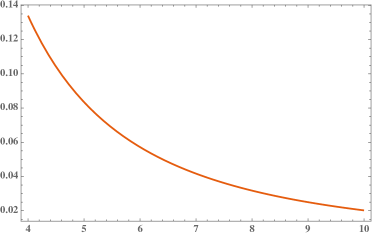
(a) right side of Inequality (3) for $\mu_{2}$ with $j=1$

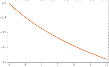
(b) Log of right side of Inequality (3) for $\mu_{2}$ with $j=1$

Figure 1: Error bound according to Corollary 3 for $\mu_{2}$ for values of $M$ on the horizontal axes. The vertical axis for the graph on the left is the right side of Inequality (3), and the vertical axis on the right is the logarithm of the right side of Inequality (3).

Corollary 4.

Under the assumptions of Theorem 6 with $j=2$. Then, in the notation of Eqs.(2.1), (2.3), for $M\geq 4$,

$$\frac{1}{A_{2}B_{2}}\left|\mu_{k}-\sum_{m=0}^{M}\sum_{\ell=m}^{k+m}\alpha_{k+2m-\ell}\beta_{\ell}A_{m,k+2m,\ell}\right|$$

$$\quad\leq 4\frac{3(k+2M-4)^{2}\left[(k+2M-4)\log\left(\frac{k+M-1}{M-3}\right)-2(k+2)\right]+4(k+2)^{3}}{9(k+2)^{2}(k+2M-4)^{3}\sqrt{(M-3)(k+M-1)}}$$ (3.20)

Proof.

From Eq.(3.12) with $j=2$,

$$\left|\mu_{k}-\sum_{m=0}^{M}\sum_{\ell=m}^{k+m}\alpha_{k+2m-\ell}\beta_{\ell}A_{m,k+2m,\ell}\right|$$

$$\qquad\qquad\leq\sum_{m=M+1}^{\infty}\int_{m-1}^{k+m+1}\frac{A_{2}B_{2}dx}{(k+2m-x-2)^{\frac{5}{2}}(x-2)^{\frac{5}{2}}}$$ (3.21)

$$\qquad\qquad=4A_{2}B_{2}\sum_{m=M+1}^{\infty}\frac{(k+2)\left(k^{2}+4k(3m-8)+12(m-4)m+40\right)}{3((m-3)(k+m-1))^{3/2}(k+2m-4)^{4}}$$

$$\qquad\qquad\leq 4A_{2}B_{2}\int_{M}^{\infty}\frac{(k+2)\left(k^{2}+4k(3m-8)+12(m-4)m+40\right)dm}{3((m-3)(k+m-1))^{3/2}(k+2m-4)^{4}},$$

where in the last step, we require $M\geq 4$. This last integral may be bounded as follows,

$$\int_{M}^{\infty}\frac{(k+2)\left(k^{2}+4k(3m-8)+12(m-4)m+40\right)dm}{3((m-3)(k+m-1))^{3/2}(k+2m-4)^{4}}r$$ (3.22)

$$\leq\frac{k+2}{3\sqrt{(M-3)(k+M-1)}}\int_{M}^{\infty}\frac{\left(k^{2}+4k(3m-8)+12(m-4)m+40\right)dm}{(m-3)(k+m-1)(k+2m-4)^{4}}$$

$$=\frac{k+2}{3\sqrt{(M-3)(k+M-1)}}\left[-\frac{2}{(k+2)^{2}(k+2M-4)}+\frac{4}{3(k+2M-4)^{3}}+\frac{\log\left(\frac{k+M-1}{M-3}\right)}{(k+2)^{3}}\right]$$

$$=\frac{k+2}{3\sqrt{(M-3)(k+M-1)}}\left[\frac{3(k+2M-4)^{2}\left((k+2M-4)\log\left(\frac{k+M-1}{M-3}\right)-2(k+2)\right)+4(k+2)^{3}}{3(k+2)^{3}(k+2M-4)^{3}}\right]$$

$$=\frac{3(k+2M-4)^{2}\left((k+2M-4)\log\left(\frac{k+M-1}{M-3}\right)-2(k+2)\right)+4(k+2)^{3}}{9(k+2)^{2}(k+2M-4)^{3}\sqrt{(M-3)(k+M-1)}}$$

The result now follows by combining Eqs.(3) and (3.22). ∎

Below we plot the right side of Inequality (4) for $k=2$, , which can be viewed as a kind of relative error.

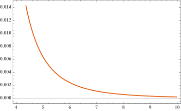
(a) Right side of Inequality (4) for $\mu_{2}$ with $j=2$

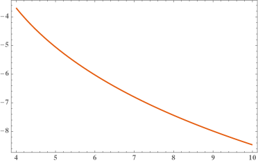
(b) Log of right side of Inequality (4) for $\mu_{2}$ with $j=2$

Figure 2: Error bound according to Corollary 4 for $\mu_{2}$ for values of $M$ on the horizontal axes. The vertical axis for the graph on the left is the right side of Inequality (4), and the vertical axis on the right is the logarithm of the right side of Inequality (4).

4 Application

Our goal is to use Legendre polynomial expansions given by Eqs. (2.1)-(2.23) to solve semi-analytically a class of nonlinear partial differential equations with polynomial nonlinearity of degree 2.

4.1 Model Prototype

Throughout this section, we consider the following class of nonlinear initial boundary value problem (IBVP),

$$(\text{IBVP})\quad \frac{\partial T}{\partial t}=\frac{\partial}{\partial x}\left[(1-x^{2})\frac{\partial T}{\partial x}\right]+c_{1}T^{2}+f(x,t)$$ (4.1)

$$(\text{IBVP})\quad \frac{\partial}{\partial x}T(-1,t)=\frac{\partial}{\partial x}T(1,t)=0$$ (4.2)

$$(\text{IBVP})\quad T(x,0)=g(x)$$ (4.3)

where $f(x,t)$, $g(x)$ are two sufficiently regular functions and $c$ is a given positive constant. The nonlinear term here is a quadratic monomial.

4.2 Solution Methodology

Our approach here is to use the Legendre expansions given by Eqs. (2.1) and (2.23) and reformulate IBVP as initial value problem that incurs a system of ordinary differential equations, which is a more simple problem from a numerical view point. To this end, we assume the functions $f$ and $g$ to admit the Legendre expansions:

$$f(x,t)=\sum_{n=0}^{\infty}d_{n}(t)P_{n}(x),\qquad g(x)=\sum_{n=0}^{\infty}c_{n}P_{n}(x),$$ (4.4)

We also assume that the sought-after solution $T$ of IBVP can be represented by the following Legendre series:

$$T(x,t)=\sum_{n=0}^{\infty}a_{n}(t)P_{n}(x).$$ (4.5)

Hence, using the truncated Legendre expansion for $T^{2}$ yields:

$$\Big{(}T(x,t)\Big{)}^{2}\approx\sum_{n=0}^{N}b_{n}(t)P_{n}(x),$$ (4.6)

where the $b_{n}$ are the coefficients in the Fourier-Legendre expansion given by Eq.(2.23).

Hence, substituting expansions (4.4)-(4.6) into IVBP allows the determination of the Legendre coefficients $a_{n}$ by solving the following initial value problem (IVP),

$$(IVP)\quad\begin{cases}a_{n}^{\prime}(t)&=-n(n+1)a_{n}(t)+c\,b_{n}(t)+d_{n}(t)\\[4.30554pt] a_{n}(0)&=c_{n}\end{cases}\quad n=0,\cdots,N$$ (4.7)

The resulting IVP is a system of nonlinear ODEs. Consequently, as stated earlier, the use of the Legendre expansions for both $T$ and $T^{2}$ results in a reduction of the numerical complexity to the requirement to solve a system of ODEs instead of a nonlinear PDE problem. We used the Runge-Kutta method of order 4 to solve the IVP. More specifically, we used the Mathematica^® software package NDSolve [14]. Once we numerically determine the coefficients $a_{n}$, we evaluate $T_{N^{\prime}}(x,t)$, the partial sum of the series (4.5) as follows:

$$T_{N^{\prime}}(x,t)=\sum_{n=0}^{N^{\prime}}a_{n}(t)P_{n}(x)$$ (4.8)

where the integer $N^{\prime}$ ($N^{\prime}\leq N$) is chosen to be smallest integer such that the values of $T_{N^{\prime}}(x,t)$ remain invariant as the values of $N^{\prime}$ increase.

4.3 Illustrative Numerical Results

We assess in this section the performance efficiency of the proposed solution methodology. Due to space limitations, we present results obtained in the case where the solution $T$ of IBVP is given by:

$$T(x,t)=e^{x^{2}-t-2}$$ (4.9)

In this case, the constant $c$ and the functions $f$ and $g$ are set to be:

$$\begin{cases}\begin{aligned} c&=1,\\ f(x,t)&=e^{x^{2}-t-2}(4x^{4}+2x^{2}-3)-e^{2x^{2}-2t-4},\\ g(x)&=e^{x^{2}-2}\end{aligned}\end{cases}$$ (4.10)

Other examples highlighting the salient features of the proposed solution methodology can be found in [15]. The obtained results in the case where $T$ is given by (4.9) are reported in Figures (3)-(5). The following two observations are noteworthy.

• Figure (3) provides a comparison between the exact Legendre coefficients of $T$ and the computed ones obtained by solving the IVP for Legendre coefficients of low-orders $n=0$ to $4$, medium-orders $n=6$ to $10$, and high-orders $n=20$ to $30$. These results show the curves corresponding to the exact values and the computed ones are undistinguishable at all times $t$. The relative errors in the euclidean norm between these curves remain at all times and for all orders less than $1\%$. Note that we have not represented the coefficients corresponding to odd values of $n$ as they are all zero since the solution $T$ given by (4.9) is an odd function with respect of the spatial variable $x$.

• Figure (4) depicts a comparison between the exact solution $T$ and the truncated sum $T_{N^{\prime}}$ given by (4.8) for different values of $N^{\prime}$ and at different times $t$ represented as multiples of the time step $\Delta t=0.01$. Note that at $t=4000\Delta t$, the solution $T$ reaches its equilibrium which is $0$ and therefore that there is no need to go further in time. These results reveal that using only $6$ terms in the truncated sum ($N^{\prime}=6$) allows us to retrieve the solution $T$ with $T_{N^{\prime}}$ at all times with an impressive accuracy level, as reported in Figure (5). Indeed, Figure (5) depicts, at each time $t^{m}=m\Delta t$ (m = 100, 500, 1000, 2000, 3000, 4000), the effect of $N^{\prime}$, the number of terms left in the partial sum given by (4.8), on the relative error given by:

  $$\frac{\|T(x,t^{m})-T_{N^{\prime}}(x,t^{m})\|_{2}}{\|T(x,t^{m})\|_{2}}=\displaystyle\frac{\left(\displaystyle\sum_{j=1}^{M}|T(x_{j},t^{m})-T_{N^{\prime}}(x_{j},t^{m})|^{2}\right)^{1/2}}{\left(\displaystyle\sum_{j=1}^{M}|T(x_{j},t^{m})|^{2}\right)^{1/2}},$$

where $T$ (resp. $T_{N^{\prime}}$) is given by (4.9) (resp. (4.8)) and $x_{j}=j\Delta x$, with $\Delta x$ being the spatial step. Note that $\Delta x=0.005$.

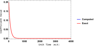
(a) $n=0$

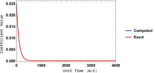
(b) $n=4$

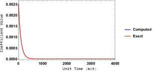
(c) $n=6$

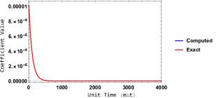
(d) $n=10$

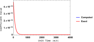
(e) $n=20$

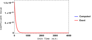
(f) $n=30$

Figure 3: Legendre coefficient values: Exact vs Computed

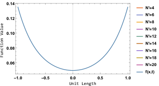
(a) $t=100\Delta t$

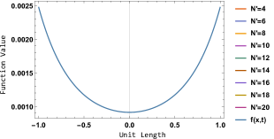
(b) $t=500\Delta t$

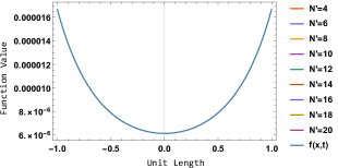
(c) $t=1000\Delta t$

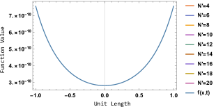
(d) $t=2000\Delta t$

(e) $t=3000\Delta t$

(f) $t=4000\Delta t$

Figure 4: Exact solution of IBVP vs. Truncated computed series. Sensitivity to the sum truncation $N^{\prime}$ at various times

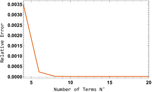
(a) $t=100\Delta t$

(b) $t=500\Delta t$

(c) $t=1000\Delta t$

(d) $t=2000\Delta t$

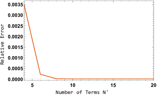
(e) $t=3000\Delta t$

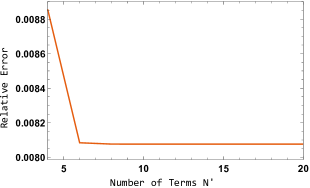
(f) $t=4000\Delta t$

Figure 5: Exact solution of IBVP vs. Truncated computed series. Sensitivity of the relative errors to the truncated order $N^{\prime}$ at various time

5 Concluding Remarks

With mild restrictions on the functions $f$ and $g$, with respective Fourier-Legendre coefficients $\{\alpha_{n}\}$ and $\{\beta_{n}\}$, we have shown that the Fourier-Legendre coefficients $\{\mu_{k}\}$ of $f\cdot g$ are given by Eq.(2.44). A bound on the rate of convergence of that series, depending on the smoothness of $f$ and $g$, is given by Theorem 6 together with its two corollaries, and bounds on the rate of convergence of the Fourier-Legendre series of $f\cdot g$ are given in Theorems 4 and 5. Our formulas may be iterated in a straightforward way to determine the Fourier-Legendre coefficients of $f^{p}(x)$ in terms of those for $f(x)$ for any positive integer $p$.

Our motivation for proving the results of Sections 2 and 3 was to apply them to finding solutions to PDEs with polynomial nonlinearities. To that end, we demonstrated in Section 4 that the search for the solution of such a PDE in the form of a Fourier-Legendre series leads to an ordinary differential equation (ODE) system in which the unknowns are the Fourier-Legendre coefficients, just as for the case of linear PDEs. In contrast to the linear case, in the nonlinear PDE case the resulting ODE is also nonlinear. Difficulties in solving this nonlinear ODE are overcome in large measure by the rapid convergence of the solution series and of the corresponding series for the nonlinear term. We showed that a high degree of accuracy is achieved by solving this system for only a few coefficients, essentially a reduced, or truncated, ODE system. We note that the resulting reduced ODE system can be solved by any preferred numerical scheme for ODEs. To our knowledge, this is the first use of Fourier-type expansions to solve semi-analytically a nonlinear PDE problem.

This example, along with others studied by the third listed author of this paper in [15], highlights the potential of this semi-analytical solution methodology for providing solutions that can serve as reference solutions to assess the accuracy level of numerical methods when solving this class of equations with non constant coefficients. In addition, we expect that this approach can be successful for solving PDEs with polynomial nonlinearity of higher degrees such as PDEs arising in global climate models. In such models, outgoing long wave radiation is modeled by a term proportional to the fourth power of temperature (the unknown function of position and time), according to the Stefan-Boltzmann law, and lateral heat diffusion may be modeled by the same term as in the nonlinear PDE we solved in Section 4 [16, 17].

Acknowledgement. The authors thank Cord Perillo for helpful discussions related to this research.

References

[1] E. Turkel, Boundary conditions and iterative schemes for the Helmholtz equation in unbounded regions, in: F. Magoules (Ed.),
Computational Methods for Acoustic Problems, Saxe-Coburg Publications, Stirlingshire (UK) (2009), pp. 127-158.
[2] H. Barucq , R. Djellouli R., and E. Estecahandy, Efficient DG-like formulation equipped with curved boundary edges for solving elasto-acoustic scattering problems, International Journal for Numerical Methods in Engineering, 98 (10) (2014), pp. 747-780.
[3] R. Dautray and J. L. Lions, Evolution Problems II, In: Mathematical Analysis and Numerical Methods for Science and Technology, Springer-Verlag, Vol. 6, (2000).
[4] P. G. Ciarlet and J. L. Lions, Techniques of Scientific Computing (Part 2), In: Handbook of Numerical Analysis, Elsevier, Vol. 5, (1997).
[5] Stone, M. H., Developments in Legendre Polynomials, Ann. Math., Second Series, Vol. 27 (4) (1926), pp. 315-329.
[6] M. Abramowitz and I. A. Stegun, Handbook of Mathematical Functions with Formulas, Graphs, and Mathematical Tables, Dover Publications Inc., Reprint of the 1972 edition: New York (1992).
[7] J. C. Adams, On the Expression of the Product of any two Legendre’s Coefficients by means of a Series of Legendre’s Coefficients, Proc. Roy. Soc., XXVII (1878), p. 63 ; also Collected Scientific Papers, I, p. 187
[8] W. N. Bailey, On the product of two Legendre polynomials, Mathematical Proceedings of the Cambridge Philosophical Society Vol. 29, Issue 2 (1933), p. 173-177
[9] J. Dougall, The Product of Two Legendre Polynomials, Proceedings of the Glasgow Mathematical Association, 1(3), 121-125. (1953) doi:10.1017/S2040618500035590
[10] W. A. A-Salam, On the product of two Legendre polynomials, Mathematica Scandinavica, Vol. 4 (2) (1957), pp. 239-242.
[11] H. Wang, A new and sharper bound for Legendre expansion of differentiable functions, Applied Mathematics Letters, 85 (2012), pp. 85-92, doi:10.1016/j.aml.2018.05.022 doi:10.1016/j.aml.2018.05.022.
[12] H. L. Royden, Real Analysis, 3d edition, Macmillan Publishing Co., New York (1988), see Chapter 5.
[13] R. B. Saxena, Expansion of continuous differentiable functions in Fourier Legendre series, Can. J. Math., 19 (1967), pp. 823-827.
[15] M. Levy, Legendre Expansions and Nonlinear Partial Differential Equations with Diffusion, Master’s thesis dissertation, California State University, Northridge (2020).
[16] T. Stocker, Introduction to Climate Modelling, Springer-Verlag, Berlin Heidelberg (2011)
[17] R. T. Pierrehumbert, Principles of Planetary Climate, Cambridge University Press (2010)