Preprint
THE INFLUENCE OF DEFLECTIONS ON THE STATIC AND DYNAMIC BEHAVIOUR OF MASONRY COLUMNS

Abstract.

This paper studies the influence of bending deflections on the structural behaviour of masonry columns. Some explicit solutions are presented, and the combined effects of the constitutive and geometric nonlinearities are investigated through an iterative numerical procedure. The results show that considering second-order effects affects both the collapse load and the dynamical properties of masonry beams significantly.

1. Introduction

Masonry buildings are unable to withstand loads with large eccentricities. Ancient masonry constructions are mainly designed to constrain the compressive force inside the elements’ section, while large tensile stresses are concentrated in the wooden and metallic parts. On the other hand, bending is always present in masonry elements. When the axial force is applied outside the central nucleus of inertia of a masonry beam, there is a reduction of the section’s stiffness, and the behaviour of the beam becomes nonlinear. Many constitutive equations have been proposed during the last century to describe the peculiar behaviour of unreinforced masonry materials, which are essentially unable to withstand tensile stresses (see [1], [15] for a review). More recently, the problem of bending in masonry has been addressed by several authors, mainly in the framework of earthquake engineering, being masonry constructions prone to seismic actions.

When deformation is taken into account in the equilibrium equations, geometric and constitutive nonlinearities are coupled, and the effects of bending are consequently amplified. First investigations on the stability of masonry pillars date back to the Seventeenths, with the studies [13], [6], and [7], and successively recalled in [2], [3], [4]. In all these studies, some explicit solutions are proposed to determine the collapse load of masonry pillars subjected to eccentric loads. In [14], [20] some iterative procedures are shown to evaluate the effects of deformation on the equilibrium of simple masonry elements; [20] also presents the results of an experimental campaign on masonry panels subjected to transverse and axial loads. In [19], a finite–element analysis is proposed to evaluate the equilibrium of masonry beams in the presence of geometric nonlinearities. The effects of large deformations, together with those of the construction phases, are taken into account in the finite–element analysis conducted in [21] to assess the static conditions of the Mallorca cathedral.

The correlation between changes in the natural frequencies and the presence of structural damage [23], [12], [11], confirmed by many dynamic monitoring campaigns [8], makes it interesting to investigate how cracks affect the dynamic behaviour of structures. As far as slender structures are concerned, the influence of fractures on the modal properties of beams has been addressed and modelled in several papers, and a comprehensive list of references is reported in [16].

This paper investigates the influence of geometric nonlinearity on the static and dynamic behaviour of Euler-Bernoulli beams made of a masonry-like material [10]. The invertibility of the moment-curvature function allows determining the explicit expression of the transverse displacement in masonry cantilever beams subjected to prescribed forces applied at the free end. Two cases are addressed: in the former (case (a)) the beam is subjected to an eccentric normal load N, in the latter (case (b)) the axial force N is applied along with a horizontal load H. The knowledge of the normal force and bending moment along the beam’s axis makes it possible to calculate the deflection while considering both material and geometric nonlinearities. When second-order effects are taken into account, the nonlinear differential equation linking deflection and curvature is integrated via an iterative scheme, thus providing response curves analogous to those available in the literature [2], [13]. The results of the numerical approach proposed in Section 2 are compared with those of finite–element analyses conducted with the Marc code using a concrete cracking model for masonry [17]. Section 3 is devoted to assessing the influence of geometric nonlinearity on the natural frequencies of masonry beams. The fundamental frequency of simply supported beams subjected to two different load conditions is calculated explicitly by using the results of Section 2. The dependence of the frequency on the loads is validated via the Marc code and plots of the frequency vs the eccentricity of load N and the horizontal load H are provided.

2. Some explicit solutions

Let us consider a rectilinear beam with a rectangular cross–section of height $h$ and width $b$, subjected to an axial force $N<0$. Let us denote by $E$ the Young’s modulus and by $J=bh^{3}/12$ the moment of inertia of the beam’s cross section, and let $x$ be the abscissa along the beam’s axis, $y(x)$ the beam’s transverse deflection at $x$. The beam is modelled according to the Euler-Bernoulli beam theory.

The curvature of the beam’s deflection is denoted by $\chi$ and, under the hypothesis that the rotations of the beam’s axis are small, is given by

$$\chi(x)=-\frac{d^{2}y}{dx^{2}},$$ (2-1)

where $\frac{d^{2}y}{dx^{2}}$ denotes the second derivative with respect to $x$.

The bending moment $M(\chi)$ is a continuously differentiable function of $\chi$, whose second derivative is assumed to be piecewise continuous.

For a beam constituted by a masonry–like material with infinite compressive strength and zero tensile strength [10], function $M(\chi)$ is

$$M(\chi)=\begin{cases}\quad EJ\,\chi\quad&\text{for $\left|\chi\right|\leq\alpha$},\\ \quad EJ\,\alpha\operatorname{Sign}(\chi)(3-2\sqrt{\frac{\alpha}{{\left|\chi\right|}}})\quad&\text{for}\left|\chi\right|>\alpha,\end{cases}$$ (2-2)

where

$$\alpha=-\frac{2N}{Ebh^{2}}$$ (2-3)

is the curvature corresponding to the elastic limit.

Function $M(\chi)$ depicted in Figure 1 is invertible and its inverse is

$$\left|\chi(M)\right|=\begin{cases}\quad\frac{\left|M\right|}{EJ}\quad&\text{for $\left|M\right|\leq-N\,h/6$},\\ \vspace{1\baselineskip}\\ 4\,\alpha^{3}/\left(\frac{\left|M\right|}{EJ}-3\,\alpha\right)^{2}\quad&\text{for\, $\left|M\right|>-N\,h/6$}.\end{cases}$$ (2-4)

Figure 1. Bending moment $M$ versus the curvature $\chi$ for a rectangular cross–section beam with infinite compressive strength and zero tensile strength.

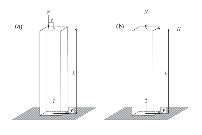
Figure 2. A cantilever beam. Case (a): eccentric axial load. Case (b): horizontal and axial loads.

Under the hypotheses above, if the bending moment $M$ and the normal force $N$ acting on the beam’s sections are known along the axis, the deflection of the beam can be easily calculated by integrating equation (2-1) with the help of (2-4). Thus, a number of explicit solutions can be obtained, some of which are reported in the following.

Let us consider the cantilever beam with length $L$ represented in Figure 2. In case (a) the beam is subjected to a normal force $N$ acting on the beam’s upper end with eccentricity $e\geq 0$. Neglecting the second–order effects, that is, ignoring the contribution of displacements and rotations on the beam’s equilibrium, the eccentricity of the axial load remains constant along the beam and, by (2-4), curvature $\chi$ is constant as well. In case (b), the beam is subjected to the vertical load $N$ and a horizontal load $H$, both acting on the upper end. Both cases, (a) and (b), are relevant in many applications concerning the static behaviour of masonry pillars. In particular, case (b) is adopted to model the seismic actions through the so–called push–over analysis. Finally, it is worth noting that the solutions for the cantilever beam of length $L$ shown in Figure 2 also hold for a simply supported beam of length $2L$; this property will be used in section 3.

2A. Case (a): cantilever beam with eccentric axial load

Let us consider the cantilever beam in figure 2 subjected to an axial force $N$ with eccentricity $e$ applied at the free end. If we neglect the geometric nonlinearity, then the curvature is constant along the axis, $\chi(x)=\mathrm{bar}\chi$, $x\in[0,L]$, where $\mathrm{bar}\chi$ has the expression given by (2-4), with $M=Ne$.

By integrating equation (2-1) and imposing the boundary conditions $y(0)=0$, $y^{\prime}(0)=0$, we obtain the transverse displacement $y(x)$ of the beam

$$y(x)=-\frac{\mathrm{bar}\chi\,x^{2}}{2},$$ (2-5)

and the displacement of the beam’s upper end

$$f_{a}=-\frac{\mathrm{bar}\chi\,L^{2}}{2}.$$ (2-6)

Equation (2-6) reduces to the well known linear value

$$\left|f_{a}\right|=\frac{\left|N\right|e}{2EJ}\,L^{2}$$ (2-7)

for $e\leq h/6$. When the eccentricity is outside the kernel, the curvature is given by the second equation of (2-4), and using (2-6), we obtain the dimensionless expression

$$\frac{\left|f_{a}\right|}{L}=\frac{1}{9\left(2e/h-1\right)^{2}}\frac{\left|N\right|}{\gamma},$$ (2-8)

with

$$\gamma=3EJ/(L\,h).$$ (2-9)

Equations (2-7) and (2-8) state that, when the eccentricity remains fixed, there is a direct proportionality between deflection and axial load, as shown in Figure 3, plotting $|f_{a}|/L$ vs $|N|/\gamma$ for different values of the eccentricity. In Figure 4, the deflection of the beam is instead plotted against the eccentricity $e$, for different values of the normal force. The figure highlights the stiffness decay of the beam, when the eccentricity increases.

The analytical solutions have been compared with results obtained via the Marc code [17]. In the numerical simulation, the nonlinear concrete cracking model is chosen to simulate masonry, with a tensile strength of $1\cdot 10^{3}\text{\,}\mathrm{Pa}$ and a Young’s modulus $E=$3\cdot 10^{9}\text{\,}\mathrm{Pa}$$, mass density $\rho=$1800\text{\,}\mathrm{k}\mathrm{g}\mathrm{/}\mathrm{m}^{3}$$, Poisson’s ratio $\nu=0.2$. The finite element model was built by using bi–linear thick shell elements (element n. 75 of Marc library).

The results of the finite element analysis, represented by dotted lines are reported in figures 3 and 4, along with the analytical counterparts. Numerical and analytical simulations provide very similar results. For small eccentricities, the numerical solution appears slightly stiffer than the analytical one, because of the low but not null tensile strength adopted in the constitutive equation available in the Marc code.

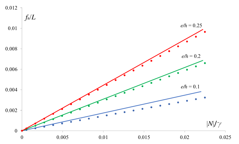
Figure 3. Case (a): deflection of a masonry–like cantilever beam $f_{a}/L$ vs normal force $|N|/\gamma$ for different values of the eccentricity.

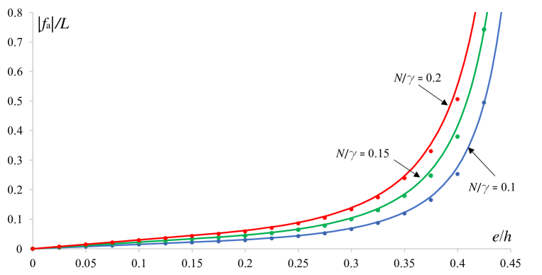
Figure 4. Case (a): deflection $f_{a}$ of a masonry–like cantilever beam vs the eccentricity $e$ acting on the beam, for different values of the ratio $\left|N\right|/\gamma$.

If we take into account the second–order effects, while assuming that (2-1) still holds, we can write the beam’s curvature as follows

$$\left|\chi(x)\right|=\begin{cases}\quad\frac{\left|N\right|}{EJ}\left(e+\left|y(L)-y(x)\right|\right)\quad&\text{for $e+\left|y(L)-y(x)\right|\leq h/6$},\\ \vspace{1\baselineskip}\\ 4\,\alpha^{3}/\left(\frac{\left|N\right|}{EJ}\left(e+\left|y(L)-y(x)\right|\right)-3\,\alpha\right)^{2}\quad&\text{for\, $e+\left|y(L)-y(x)\right|>h/6$}.\end{cases}$$ (2-10)

As shown by equations (2-10), the curvature is no more constant along the beam’s axis. The differential equations (2-1), (2-10) can be numerically solved via the following iterative scheme [24]

$$\frac{d^{2}y^{(n+1)}}{dx^{2}}=-\chi^{(n)},$$ (2-11)

$$\left|\chi^{(n)}(x)\right|=\begin{cases}\quad\frac{\left|N\right|}{EJ}\left(e+\left|y^{(n)}(L)-y^{(n)}(x)\right|\right)\quad&\text{for $e+\left|y^{(n)}(L)-y^{(n)}(x)\right|\leq h/6$},\\ \vspace{1\baselineskip}\\ 4\,\alpha^{3}/\left(\frac{\left|N\right|}{EJ}\left(e+\left|y^{(n)}(L)-y^{(n)}(x)\right|\right)-3\,\alpha\right)^{2}\quad&\text{for\, $e+\left|y^{(n)}(L)-y^{(n)}(x)\right|>h/6$},\end{cases}$$ (2-12)

and

$$y^{(0)}(x)=0,\,\,\,\,x\in[0,L].$$ (2-13)

The algorithm converges when the difference between deflection at step $n+1$ and deflection at step $n$, $(n>0)$ falls under a fixed residual value $\varepsilon$

$$\max\limits_{x\in[0,L]}\frac{\left|y^{(n+1)}(x)-y^{(n)}(x)\right|}{\left|y^{(n)}(x)\right|}<\varepsilon.$$ (2-14)

The maximum eccentricity along the beam’s axis is attained at $x=0$ and reaches, at the final step $n_{max}$, the value

$$e_{max}=e+y^{(n_{max})}(L).$$ (2-15)

Let us define the quantities

$$N_{E}=\pi^{2}\frac{EJ}{(2L)^{2}},$$ (2-16)

$$u=\frac{h}{2}-e_{max},$$ (2-17)

which represent, respectively, the Euler’s critical load of the cantilever beam and the distance of the axial force from the compressed edge at $x=0$. Ratio $\left|N\right|/N_{E}$ is plotted in Figure 5 against ratio $u/h$, for different values of the initial eccentricity $e$. If $e$ exceeds the limit elastic value $h/6$, the whole process takes place in the nonlinear field, while, for $e\leq h/6$, the beam, which initially behaves linearly, cracks during the process due to the geometric nonlinearity. The iteration scheme has been implemented in the Mathematica environment [18] and calculations are performed by setting the residual $\varepsilon$ (in percentage) at $0.001$ and allowing the maximum number of thirty iterations. The solutions, shown in the Figure 5 via solid lines, coincide with the explicit curves reported in [3], [13]. The results of the finite element analysis conducted via the Marc code (dots) are also reported in the figure and show an excellent agreement with those of algorithm (2-11)–(2-13). The finite element analysis exploits the arc–length method [17] to evaluate the beam’s behaviour after buckling, while the algorithm is not able to follow the post–critical behaviour of the system.

Figure 6 shows the dimensionless load–displacement curves for the masonry–like case (dashed line), and under the combined effect of the constitutive and geometric nonlinearity (continuous line). Dots represent the results of the numerical simulation performed via Marc code. The curves depend on the value of the ratio between the eccentricity $e$ at the top of the column and the height $h$ of the section, which is here set to $1/5$. The abscissa $\left|f_{a}\right|/L$ represents the deflection of the beam’s top to the beam’s length. The effects of cracking on the stiffness of the beam are evident. However, considering only the constitutive nonlinearity, it does not allow modelling the collapse, which is captured instead when the effects of deformation are taken into account in the equilibrium equations.

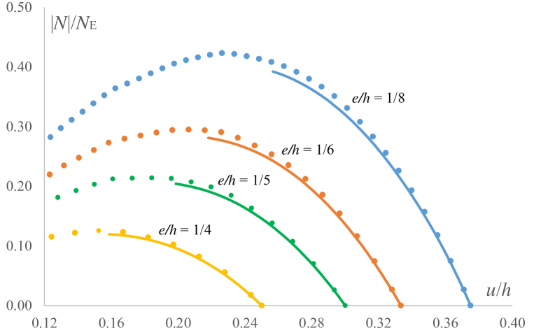
Figure 5. Case (a) : ratio $\left|N\right|/N_{E}$ vs ratio $u/h$ for different values of the initial eccentricity $e$. From the left: $e/h=1/4$, $e/h=1/5$, $e/h=1/6$, $e/h=1/8$.

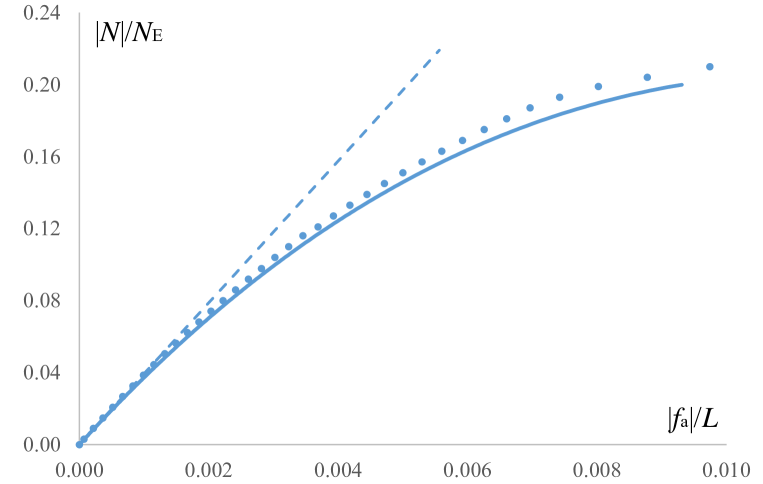
Figure 6. Case (a): load–displacement curves for $e/h=1/5$. Masonry–like material (dashed curve); masonry–like material with geometric nonlinearity (continuous curve); finite–element simulation (dots).

2B. Case (b): cantilever beam with axial and horizontal loads

Let us consider the cantilever beam subjected to an axial force $N$ and a horizontal force $H$, applied to the upper end. The eccentricity of the normal force is no more constant along the beam’s length; in fact, in the case of small deflection the first–order bending moment $M$ has the expression

$$M(x)=H(L-x).$$ (2-18)

The horizontal force $H$, supposed nonnegative, ranges in the interval $[0,H_{max}]$, where

$$H_{max}=\frac{\left|N\right|h}{2L}$$ (2-19)

is the load corresponding to which the normal force $N$ is applied at the edge of the base section.

Thus, let us define the abscissa $x_{0}$ as the position along the beam’s length in which the curvature takes the limit elastic value $\alpha$ given in (2-3), that is

$$\left|\chi(x_{0})\right| =\alpha,$$ (2-20)

$$\left|M(x_{0})\right| =\left|N\right|h/6.$$ (2-21)

Equations (2-18) and (2-21) give

$$x_{0}=L-\frac{\left|N\right|h}{6H}=L-\frac{\alpha}{k},$$ (2-22)

with

$$k=\frac{H}{EJ}.$$ (2-23)

If the beam is all in the linear elastic field, that is, if

$$H\leq\frac{\left|N\right|h}{6L},$$ (2-24)

then $x_{0}$ is zero, and the solution to equation (2-1) coincides with the linear elastic deflection.

For $x_{0}>0$, from (2-4), we get the expression of the curvature $\chi$ along the axis

$$\chi(x)=\begin{cases}\quad\frac{H(L-x)}{EJ}\quad&\text{for $x\geq x_{0}$},\\ \vspace{1\baselineskip}\\ 4\,\alpha^{3}/\left(\frac{H(L-x)}{EJ}-3\,\alpha\right)^{2}\quad&\text{for\, $x<x_{0}$}.\end{cases}$$ (2-25)

Therefore, the solution of equation (2-1) splits into two parts, $y=y_{1}(x)$ for $x\leq x_{0}$, $y=y_{2}(x)$ for $x>x_{0}$, where $y_{1}$ and $y_{2}$ have the following explicit expressions,

$$y_{1}(x)=c_{1}+c_{2}x+\frac{4\alpha^{3}}{k^{2}}\,\log\big{(}k(x-L)+3\alpha\big{)}\quad\text{for $x\leq x_{0}$},$$ (2-26)

$$y_{2}=c_{3}+c_{4}x-\frac{kL}{2}x^{2}+\frac{k}{6}x^{3},\quad\text{for\, $x>x_{0}$},$$ (2-27)

with $k$ given by (2-23). The conditions

$$\begin{cases}y_{1}(x_{0})=y_{2}(x_{0}),\\ \vspace{1\baselineskip}\\ y^{\prime}_{1}(x_{0})=y^{\prime}_{2}(x_{0}),\\ \vspace{1\baselineskip}\\ y_{1}(0)=y^{\prime}_{1}(0)=0.\\ \end{cases}$$ (2-28)

allow determining the constants

$$c_{1}=-\frac{4\alpha^{3}}{k^{2}}\log(3\alpha-kL),$$ (2-29)

$$c_{2}=-\frac{4\alpha^{3}}{k}\frac{1}{(3\alpha-kL)},$$ (2-30)

$$c_{3}=-\frac{(kL-\alpha)^{3}}{2k(3\alpha-kL)},$$ (2-31)

$$c_{4}=-\frac{1}{6k^{2}}\left[k^{3}L^{3}+9kL\alpha^{2}-10\alpha^{3}-24\alpha^{3}\big{(}\log{2\alpha}-\log{(3\alpha-kL)}\big{)}\right].$$ (2-32)

The deflection of the top of the cantilever beam takes thus the expression

$$f_{a}=-\frac{\alpha^{3}}{3k^{2}(3\alpha-kL)}\left\{17kL-15\alpha-12(3\alpha-kL)\left[\log{2\alpha}-\log{(3\alpha-kL)}\right]\right\},$$ (2-33)

and the problem is governed by the curvature

$$\zeta=3\alpha-kL.$$ (2-34)

It is an easy matter to prove that

$$\zeta=3\alpha(1-\left|M(0)\right|/M_{max}),$$ (2-35)

with $M(0)$ the bending moment at the beam’s base, and

$$M_{max}=H_{max}\,L$$ (2-36)

the maximum bending moment sustainable by the beam’s section.

The curvature $\zeta$ tends to zero when $\left|M(0)\right|$ tends to $M_{max}$. Correspondingly, the deflection (2-33) of the beam tends to infinity. When $\left|M(0)\right|$ tends to the limit linear value $\left|N\right|h/6$, then $k=\alpha/L$ and thus $\zeta$ tends to $2\alpha$. In this case the deflection of the beam coincides with the well known value $\left|f_{a}\right|=kL^{3}/3$.

By introducing the quantities

$$\mathrm{bar}k=kL^{2},\,\,\,\,\,\,\,\mathrm{bar}\alpha=\alpha L,\,\,\,\,\,\,\,\,\mathrm{bar}\zeta=\zeta L,$$ (2-37)

equation (2-33) takes the dimensionless form

$$\frac{f_{a}}{L}=-\frac{\mathrm{bar}\alpha^{3}}{3\mathrm{bar}k^{2}\mathrm{bar}\zeta}\left(17\,\mathrm{bar}k-15\,\mathrm{bar}\alpha-12\,\mathrm{bar}\zeta\log{\frac{2\mathrm{bar}\alpha}{\mathrm{bar}\zeta}}\right).$$ (2-38)

In figure 7 some load–displacement curves are shown (push–over curves) for different values of the normal force acting on the beam’s section (measured by the dimensionless limit elastic curvature $\mathrm{bar}\alpha$).

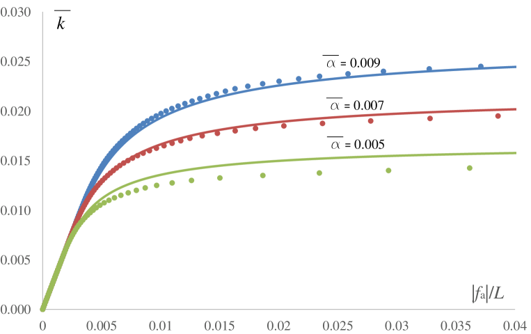
Figure 7. Case (b): push–over curves for different values of $\mathrm{bar}\alpha$. Dots represent the finite–element solution.

As done for case (a), to take into account the geometric nonlinearity we can adopt the following iterative scheme

$$\frac{d^{2}y^{(n+1)}}{dx^{2}}=-\chi^{(n)},$$ (2-39)

$$\left|\chi^{(n)}(x)\right|=\begin{cases}\quad\frac{\left|H\right|}{EJ}(L-x)+\frac{\left|N\right|}{EJ}\left|y^{(n)}(L)-y^{(n)}(x)\right|\quad&\text{for $x\geq x_{0}^{(n)}$},\\ \vspace{1\baselineskip}\\ 4\,\alpha^{3}/\left(\frac{\left|H\right|}{EJ}(L-x)+\frac{\left|N\right|}{EJ}\left|y^{(n)}(L)-y^{(n)}(x)\right|-3\,\alpha\right)^{2}\quad&\text{for\, $x<x_{0}^{(n)}$},\end{cases}$$ (2-40)

$$y^{(0)}(x)=0,$$ (2-41)

$x_{0}^{(0)}$ is given by (2-22), and $x^{(n)}_{0}$ is root of the equation

$$\left|H\right|(L-x)+|N|\left|y^{(n)}(L)-y^{(n)}(x)\right|=\frac{|N|h}{6}.$$ (2-42)

As for the previous case, iterations (2-39)– (2-42) are repeated until the difference between two consecutive deflections becomes smaller than a prescribed residual value $\varepsilon$.

Figure 8 shows the push–over curves for $\mathrm{bar}\alpha=9\cdot 10^{-3}$ in the linear elastic case (dash-dotted line), in the masonry–like case (dashed line), and in the masonry–like case with geometric nonlinearity (continuous line), via algorithm (2-39)–(2-41). Calculations has been performed setting the residual $\varepsilon$ (percentage) to 0.001 and the maximum number of iterations to 30. Dots represent the results of the finite–element analysis. Second–order effects cause a significant change in the system’s response to the horizontal load; the collapse load $H_{g}$ is about one half of the maximum horizontal load $H_{max}$ admissible in the masonry–like solution. Figure 9 shows the ratio between $H_{g}$ and $H_{max}$ vs the axial force $N$ (in the abscissa the ratio $\left|N\right|/N_{E}$). The figure highlights the reduction of the beam’s strength when the geometric nonlinearity is taken into account. Results of the finite–element analysis are also reported in the figure (dots). As a results of the different model adopted, the collapse load evaluated by the Marc code is always slightly larger than that evaluated via the masonry–like constitutive equation.

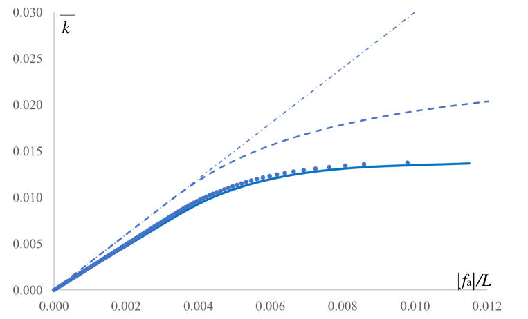
Figure 8. Case (b): push–over curves for $\mathrm{bar}\alpha=9\cdot 10^{-3}$. linear elastic solution (dash–dotted line); masonry–like solution (dashed line); masonry–like solution with geometric nonlinearity (continuous line); finite–element solution (dots).

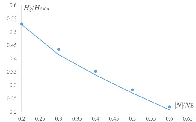
Figure 9. Case (b): ratio between the collapse load $H_{g}$ calculated by taking into account geometric nonlinearity and $H_{max}$, vs the ratio $\left|N\right|/N_{E}$, analytical results (continuous line) and finite–element results (dots).

3. Influence of geometric nonlinearity on the natural frequencies of masonry beams

The results shown in the previous section can be used to evaluate the effects of deflections on the natural frequencies of masonry beams, by using the method proposed in [9], where the fundamental frequency of a simply supported masonry beam subjected to some load conditions is calculated explicitly.

The geometry of the beam is described in figure 10, for both cases (a) and (b).

By taking into account the axial force $N$, the motion of the beam is governed by the equation

$$y_{tt}-(f(\chi))_{xx}=\left[p(x,t)+N\,y_{xx}\right]\frac{1}{\rho bh},$$ (3-1)

where $x\in[0,2L]$ is the abscissa along the beam’s axis (figure 10), $p(x,t)$ is the transverse load per unit length, and

$$f(\chi)=\frac{M(\chi)}{\rho\,b\,h}.$$ (3-2)

Let us consider, at $t=0$, a load $\mathrm{bar}p(x)$ inducing in the beam an initial deflection $\mathrm{bar}y(x)$ and curvature change $\mathrm{bar}\chi(x)$. The beam reaches the equilibrium under load $\mathrm{bar}p$, and thus

$$-\left(f(\mathrm{bar}\chi)\right)_{xx}=\left[\mathrm{bar}p(x)-N\,\mathrm{bar}\chi\right]\frac{1}{\rho bh}.$$ (3-3)

We are interested in studying the small oscillations $\delta y$ of the beam around $\mathrm{bar}y$

$$\delta y_{tt}-\left(\frac{df}{d\chi}\Bigg{|}_{\mathrm{bar}\chi}\delta\chi\right)_{xx}=-\frac{N}{\rho bh}\,\delta\chi,$$ (3-4)

where we used the approximation

$$f(\mathrm{bar}\chi+\delta\chi)\simeq f(\mathrm{bar}\chi)+\frac{df}{d\chi}\Bigg{|}_{\mathrm{bar}\chi}\delta\chi,$$ (3-5)

and condition (3-3). We assume the small oscillations $\delta y$ have the approximate expression

$$\delta y\simeq\delta a\sin\left(\frac{\pi}{2L}x\right)u(t),$$ (3-6)

with $\delta a>0$. By following the procedure described in [9], from (3-4) we get an approximation of the fundamental frequency

$$\omega^{2}\simeq\frac{2\pi^{4}}{(2L)^{5}}\int_{0}^{2L}\sin^{2}\left(\frac{\pi}{2L}x\right)\frac{df}{d\chi}\Bigg{|}_{\mathrm{bar}\chi}dx+\frac{c^{2}\pi^{4}}{(2L)^{4}}\frac{N}{N_{E}},$$ (3-7)

where

$$\frac{df}{d\chi}\Bigg{|}_{\mathrm{bar}\chi}=\begin{cases}\quad c^{2}\quad&\text{for $\left|\mathrm{bar}\chi\right|\leq\alpha$},\\ \quad c^{2}\sqrt{\frac{\alpha^{3}}{{\left|\mathrm{bar}\chi\right|}^{3}}}\quad&\text{for}\left|\mathrm{bar}\chi\right|>\alpha,\end{cases}$$ (3-8)

$c$ is the elastic constant of the beam

$$c^{2}=\frac{EJ}{\rho bh},$$ (3-9)

and $N_{E}$ is the Euler load expressed by (2-16).

If the material constituting the beam is linear elastic, by using the first equation of (3-8), equation (3-7) becomes

$$\omega^{2}=\omega_{el}^{2}\left(1-\frac{\left|N\right|}{N_{E}}\right),$$ (3-10)

with

$$\omega_{el}^{2}=\frac{c^{2}\pi^{4}}{(2L)^{4}}.$$ (3-11)

In the case of masonry–like material, first term in (3-7) takes into account both constitutive and geometric nonlinearity in the equilibrium equation (3-3); the fundamental frequency $\omega^{2}$ can be calculated by using function $\mathrm{bar}\chi$ determined via the algorithm shown in the previous sections.

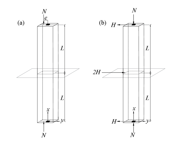
Figure 10. Simply supported scheme corresponding to cases (a) and (b).

3A. Case (a): simply supported beam with eccentric axial load

Let us consider the beam represented in figure 10. The beam is subjected to a constant axial force $N$ with eccentricity $e$. The deformation of the beam can be obtained form that of the cantilever beam of length $L$ (Case (a), subsection 2A). Thus, equation (3-7) becomes

$$\omega^{2}\simeq\frac{4\pi^{4}c^{2}}{(2L)^{5}}\int_{0}^{L}\sin^{2}\left(\frac{\pi x}{2L}\right)\sqrt{\frac{\alpha^{3}}{\left|\mathrm{bar}\chi\right|^{3}}}\,dx+\frac{c^{2}\pi^{4}}{(2L)^{4}}\frac{N}{N_{E}}\quad\text{for}\left|\mathrm{bar}\chi\right|>\alpha,$$ (3-12)

with $\left|\mathrm{bar}\chi\right|$ given by algorithm (2-11)–(2-13).

Figure 11 shows ratio $\omega/\omega_{el}$ vs ratio $e/h$, for different values of the normal force $\left|N\right|/N_{E}$ acting on the beam, and $N_{E}$ the Euler critical load given by (2-16). The black dashed curve represents the masonry–like solution without taking into account geometric nonlinearity. This last solution, as shown in [9], does not depend on the normal force. On the contrary, taking into account the effects of deflections induces a strong dependence of the solution on the normal force. In particular, as shown by Figure 11, when the ratio $\left|N\right|/N_{E}$ increases the beam’s fundamental frequency quickly decreases. For $\left|N\right|/N_{E}=0.3$ (red line in the figure), the beam approaches the collapse when the load is applied with an eccentricity of only $1/6$ of the section’s height $h$; the corresponding solution without taking into account the geometric nonlinearity (black dashed curve) remains entirely in the linear elastic field, and the fundamental frequency coincides with $\omega_{el}$.

In Figure 11 the dots represent the results of the finite–element simulation, obtained via the prestressed modal analysis procedure [17]. The figure shows a very good agreement between the results obtained via equation (3-12) and those evaluated by the finite–element code.

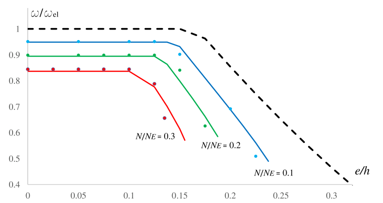
Figure 11. Case (a). Ratio $\omega/\omega_{el}$ vs $e/h$ for a masonry–like beam by taking into account the geometric nonlinearity. $\left|N\right|/N_{E}=0.3$ (red curve); $\left|N\right|/N_{E}=0.2$ (green curve); $\left|N\right|/N_{E}=0.1$ (blue curve); finite–element simulation (dots); masonry–like solution without geometric nonlinearity (dashed black line).

3B. Case (b): simply supported beam with axial and horizontal loads

Case b considers a simply supported beam of length $2L$ subjected to a concentrated load $2H$ in the mid–section, as shown in figure 10. For this structure the equivalence applies to Case (b) of subsection 2B.

The fundamental frequency of the beam can be deduced from (3-7)

$$\omega^{2}=\frac{4\pi^{4}c^{2}}{(2L)^{5}}\left(\int_{0}^{x_{0}}\sin^{2}\left(\frac{\pi x}{2L}\right)\sqrt{\frac{\alpha^{3}}{|\mathrm{bar}\chi|^{3}}}\,dx+\int_{x_{0}}^{L}\sin^{2}\left(\frac{\pi x}{2L}\right)\,dx\right)+\frac{c^{2}\pi^{4}}{(2L)^{4}}\frac{N}{N_{E}}$$ (3-13)

with $x_{0}$ the abscissa of the beam’s section in which $\left|\mathrm{bar}\chi\right|=\alpha$, and $\left|\mathrm{bar}\chi\right|$ determined via algorithm (2-39)–(2-42).

Figures 12 to 14 show the fundamental frequency $\omega/\omega{el}$ of the beam vs the horizontal force acting (ratio $H/H_{max}$), for different values of $N/N_{E}$ (ranging from 0.2 in Figure 12 to 0.4 in Figure 14). The dashed line is for the masonry–like material without geometric nonlinearity: the fundamental frequency of the beam is equal to $\omega_{el}$ for $H\leq H_{min}$ and decreases for greater values of $H$. The continuous lines show the frequency of the beam when the geometric nonlinearity is also taken into account. In this case, the frequency begins to decrease when the horizontal force is lower than $H_{min}$ and falls down when the structures reaches the collapse load $H_{g}$ (see Figure 9). For $N=0.4\,N_{E}$ the collapse load $H_{g}$ is essentially equal to $H_{min}$ and, thus, the geometric nonlinearity cuts the frequency while the corresponding masonry–like curve is still in the linear field. The figures present also the results of the finite–element simulation (dots) conducted via the prestressed modal analysis implemented in [17].

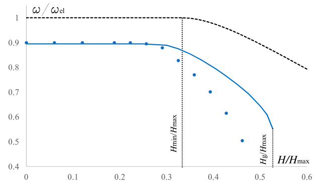
Figure 12. Case (b): ratio $\omega/\omega_{el}$ vs $H/H_{max}$ for a masonry–like beam and $\left|N\right|/N_{E}=0.2$. Masonry–like without geometric nonlinearity (dashed line); masonry–like by taking into account geometric nonlinearity (continuous line); finite–element simulation (dots).

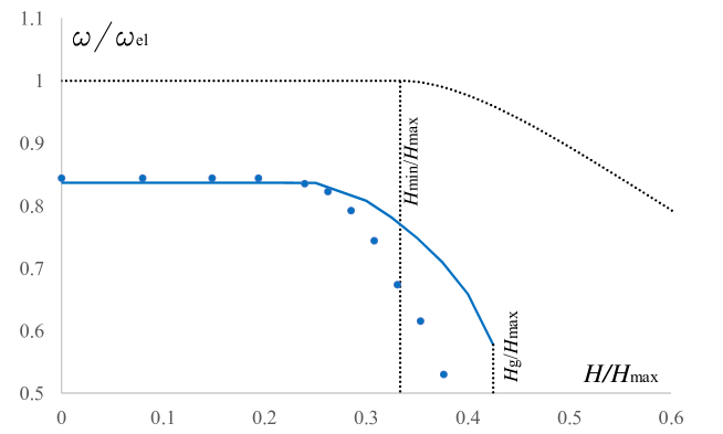
Figure 13. Case (b): ratio $\omega/\omega_{el}$ vs $H/H_{max}$ for a masonry–like beam and $\left|N\right|/N_{E}=0.3$. Masonry–like without geometric nonlinearity (dashed line); masonry–like by taking into account geometric nonlinearity (continuous line); finite–element simulation (dots).

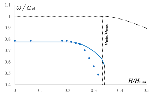
Figure 14. Case (b): ratio $\omega/\omega_{el}$ vs $H/H_{max}$ for a masonry–like beam and $\left|N\right|/N_{E}=0.4$. Masonry–like without geometric nonlinearity (dashed line); masonry–like by taking into account geometric nonlinearity (continuous line); finite–element simulation (dots).

Conclusions

The present paper investigates the influence of geometric nonlinearity on the static and dynamic behaviour of Euler- Bernoulli beams made of a masonry-like material. In the first part, the static behaviour of a cantilever beam subjected to an eccentric normal load (case (a)) and to axial and horizontal loads (case (b)) is addressed. The knowledge of the normal force and bending moment along the beam’s axis makes it possible to calculate the deflection while considering both material and geometric nonlinearities. The nonlinear differential equation that links deflection and curvature when second-order effects are taken into account is integrated via an iterative scheme. Several response curves for case (a) and push-over curves for case (b) are reported to highlight how geometric nonlinearity reduces the static performance of the beam. The second part of the paper aims to assess the influence of geometric nonlinearity on the fundamental frequency of a simply supported masonry beam. In particular, the frequency is explicitly calculated exploiting the knowledge of the beam’s deflection for the cases (a) and (b) dealt with in the first part. It is worth noting that the reduction of the fundamental frequency due to the presence of cracks is remarkably exacerbated by the geometric nonlinearity. The results concerning the static and dynamic behaviour of the beam are corroborated by finite-element analysis.

References

- [1] M. Como. Statics of historic masonry constructions. Springer Series in Solid and Structural mechanics, Book 5, Springer–Verlag, 2016.
- [2] A. De Falco and M. Lucchesi. Stability of columns with no tension strenght and bounded compressive strenght and deformability. part i: large eccentricity. International Journal of Solids and Structures 2002; 39:6191–6210.
- [3] A. De Falco and M. Lucchesi. Explicit solutions for the stability of no–tension beam–columns. International Journal of Structural stability ad Dynamics 2003; 3(2):195–213.
- [4] A. De Falco and M. Lucchesi. No tension beam-columns with bounded compressive strength and deformability undergoing eccentric vertical loads. International Journal of Mechanical Sciences 2007; 49(1): 54-74.
- [5] G. Del Piero. Constitutive equation and compatibility of the external loads for linear elastic masonry–like materials. Meccanica 1989; 24: 150-162.
- [6] R. Frisch-Fay. Stability of masonry piers. International Journal of Solids and Structures 1975; 11(2): 187–198, Elsevier.
- [7] R. Frisch-Fay. Buckling of masonry pier under its own weight International Journal of Solids and Structures, 1980; 16(5): 445–450, Elsevier.
- [8] C. Gentile, and A. Saisi (2007). A Ambient vibration testing of historic masonry towers for structural identification and damage assessment. Construction and building materials, 21(6), 1311-1321.
- [9] M. Girardi. On the natural frequencies of masonry beams Archive of Applied Mechanics, 2021; https://doi.org/10.1007/s00419-021-01887-4, Springer.
- [10] M. Girardi and M. Lucchesi. Free flexural vibrations of masonry beam-columns. Journal of Mechanics of Materials and Structures, 2010; 5(1): 143-159.
- [11] M. Girardi, C. Padovani and D. Pellegrini. Modal analysis of masonry structures. Mathematics and Mechanics of Solids, 2019; 24(3):616–636.
- [12] R. Hou, and Y. Xia (2020). Review on the new development of vibration-based damage identification for civil engineering structures: 2010-2019. Journal of Sound and Vibration, 115741.
- [13] Yokel, F. Y., Stability and capacity of members with no tensile strength, Journal of the Structural Division, ASCE, Vol. 97, No. 7, 1971, pp. 1913-1926.
- [14] L. La Mendola, and M. Papia. Stability of masonry piers under their own weight and eccentric load. Journal of Structural Engineering, 1993; 119(6), 1678–1693, ASCE.
- [15] M. Lucchesi, C. Padovani, G. Pasquinelli, N. Zani. Masonry constructions: mechanical models and numerical applications Lecture Notes in Applied and Computational Mechanics, Vol. 39, Springer–Verlag, 2008.
- [16] M. Kisa, and M.A. Gurel, M. A. (2006). Modal analysis of multi-cracked beams with circular cross section. Engineering Fracture Mechanics, 73(8), 963-977.
- [17] Marc 2014. Volume A: theory and user information. Marc and Mentat Docs.
- [18] Mathematica, Wolfram Research, Inc., https://www.wolfram.com/mathematica.
- [19] B. Pintucchi and N. Zani. Effects of material and geometric non-.linearities on the collapse load of masonry arches European Journal of Mechanics A/Solids 2009; 28: 45–61.
- [20] J.R.B. Popehn, A.E. Schultz,M. Lu and H.H.K. Stolarski, and N.J. Ojard. Influence of transverse loading on the stability of slender unreinforced masonry walls. Engineering Structures 2009; 30(10): 2830–2839, Elsevier.
- [21] P. Roca, M. Cervera, L. Pelà, R. Clemente, & M. Chiumenti. (2013). Continuum FE models for the analysis of Mallorca Cathedral. Engineering Structures, 46, 653-670.
- [22] A. Saisi, C. Gentile, and M. Guidobaldi (2015). Post-earthquake continuous dynamic monitoring of the Gabbia Tower in Mantua, Italy. Construction and Building Materials, 81, 101-112.
- [23] O.S. Salawu (1997). Detection of structural damage through changes in frequency: a review. Engineering structures, 19(9), 718-723.
- [24] G.F. Simmons (2017). Differential equations with applications and historical notes, 3rd edition, CRC Press Taylor & Francis Group.