Locally Order-Preserving Mapping for WENO Methods

Abstract

In our previous studies [17, 18], the commonly reported issue that most of the existing mapped WENO schemes suffer from either losing high resolutions or generating spurious oscillations in long-run simulations of hyperbolic problems has been successfully addressed, by devising the improved mapped WENO schemes, namely MOP-WENO-X, where “X” stands for the version of the existing mapped WENO scheme. However, all the MOP-WENO-X schemes bring about the serious deficiency that their resolutions in the region with high-frequency but smooth waves are dramatically decreased compared to their associated WENO-X schemes. The purpose of this paper is to overcome this drawback. We firstly present the definition of the locally order-preserving (LOP) mapping. Then, by using a new proposed posteriori adaptive technique, we apply this LOP property to obtain the new mappings from those of the WENO-X schemes. The essential idea of the posteriori adaptive technique is to identify the global stencil in which the existing mappings fail to preserve the LOP property, and then replace the mapped weights with the weights of the classic WENO-JS scheme to recover the LOP property. We build the resultant mapped WENO schemes and denote them as LOP-WENO-X. The numerical experiments demonstrate that the resolutions in the region with high-frequency but smooth waves of the LOP-WENO-X schemes are similar or even better than those of their associated WENO-X schemes and naturally much higher than the MOP-WENO-X schemes. Furthermore, the LOP-WENO-X schemes gain all the great advantages of the MOP-WENO-X schemes, such as attaining high resolutions and in the meantime preventing spurious oscillations near discontinuities when solving the one-dimensional linear advection problems with long output times, and significantly reducing the post-shock oscillations in the simulations of the two-dimensional problems with shock waves.

1 Introduction

In the numerical calculation of hyperbolic conservation laws in the form

$$\dfrac{\partial\mathbf{u}}{\partial t}+\nabla\cdot\mathbf{F}(\mathbf{u})=0,$$ (1)

with proper initial conditions and boundary conditions, the class of weighted essentially non-oscillatory (WENO) schemes [23, 24, 19, 12, 22], which is an evolution of the essentially non-oscillatory (ENO) schemes [8, 9, 10, 7], is widely used due to its success in using a nonlinear convex combination of all the candidate stencils to automatically achieve high-order accuracy in smooth regions and without destroying the non-oscillatory property near shocks or other discontinuities. The classic WENO-JS proposed by Jiang and Shu [12] is the most popular one of the WENO schemes. By using the sum of the normalized squares of the scaled $L_{2}-$norms of all the derivatives of $r$ local interpolating polynomials, a new measurement of the smoothness of the numerical solutions on substencils, named smoothness indicators, is devised to help to obtain $(2r-1)$th-order of accuracy from the $r$th-order ENO schemes.

It is well-known that the WENO-JS scheme is a quite successful methodology for solving problems modeled by the hyperbolic conservation laws in the form of Eq.(1). However, despite its great advantages of efficient implementation and high-order accuracy, its convergence orders dropped for many cases such as at or near critical points of order $n_{\mathrm{cp}}=1$ in the smooth regions. Here, we refer to $n_{\mathrm{cp}}$ as the order of the critical point; e.g., $n_{\mathrm{cp}}=1$ corresponds to $f^{\prime}=0,f^{\prime\prime}\neq 0$ and $n_{\mathrm{cp}}=2$ corresponds to $f^{\prime}=0,f^{\prime\prime}=0,f^{\prime\prime\prime}\neq 0$, etc. In [11], Henrick et al. pointed out that the fifth-order WENO-JS scheme fails to yield the optimal convergence order at or near critical points where the first derivative vanishes but the third derivative does not simultaneously. In the same article, they derived the necessary and sufficient conditions on the nonlinear weights for optimality of the convergence rate of the fifth-order WENO schemes and these conditions were reduced to a simpler sufficient condition by Borges et al. [1], which could be easily extended to the $(2r-1)$th-order WENO schemes [4]. Then, in order to address the drawback of the WENO-JS scheme discussed above, Henrick et al. [11] innovatively designed a mapping function satisfying the sufficient condition to achieve the optimal order of accuracy, leading to the original mapped WENO scheme, named WENO-M hereafter. Since then, obeying the similar criteria proposed by Henrick et al. [11], many different kinds of mapped WENO schemes have been successfully proposed [3, 4, 14, 28, 16, 15].

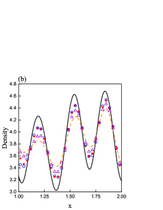
Fig. 8: Results of LOP-/MOP-/WENO-PM6 and WENO-JS on solving the Shu-Osher problem.

In [4], by rewriting the mapping function of the WENO-M scheme in a simpler and more meaningful form and then extending it to a general class of improved mapping functions, Feng et al. proposed the group of WENO-IM($k,A$) schemes and WENO-IM(2, 0.1) was recommended. WENO-IM(2, 0.1) can significantly decrease the dissipations of the WENO-M scheme leading to higher resolutions. However, in [28], Wang et al. indicated that the seventh- and ninth- order WENO-IM(2, 0.1) schemes generated evident spurious oscillations near discontinuities with a long output time. Furthermore, the present authors have reported that [16, 17], even for the fifth-order WENO-IM(2,0.1) scheme, the spurious oscillations are also produced when the grid number increases. In [3], Feng et al. found that, when the WENO-M scheme was used for solving the problems with discontinuities, its mapping function may amplify the effect from the non-smooth stencils leading to a potential loss of accuracy near discontinuities and this loss of accuracy could be accumulated when the simulating time is large. To fix this issue, two additional requirements, that is, $g^{\prime}(0)=0$ and $g^{\prime}(1)=0$ ($g(x)$ denotes the mapping function), to the original criteria in [11] was proposed and then a piecewise polynomial mapping function satisfying these additional requirements was devised. The resultant scheme was denoted as WENO-PM$k$ and $k=6$ was recommended. The WENO-PM6 scheme [3] obtained significantly higher resolution than the WENO-M scheme when computing the one-dimensional linear advection problem with long output times. However, it may generate the non-physical oscillations near the discontinuities as shown in Fig. 8 of [4] and Figs. 3-8 of [28].

Besides WENO-IM($2,0.1$) and WENO-PM6, many other modified mapped WENO schemes have been successfully proposed to enhance the conventional WENO-JS scheme’s performance, e.g., WENO-PPM$n$ [14], WENO-RM($mn0$) [28], WENO-MAIM$i$ [16], WENO-ACM [15], MIP-WENO-ACM$k$ [17] and et al. Despite that, as reported in literatures [4, 28], most of these existing modified mapped WENO schemes can hardly avoid the spurious oscillations near discontinuities, especially for long output time simulations. In addition, when computing the 2D problems with shock waves, the post-shock oscillations become very serious for most of the existing modified mapped WENO schemes [15].

It was reported [17] that, for many existing mapped WENO schemes, e.g., WENO-PM6 [3], WENO-IM(2, 0.1) [4], WENO-MAIM1 [16], MIP-WENO-ACM$k$ [17] and et al, the order of the nonlinear weights for the substencils of the same global stencil has been changed at many points in the mapping process. This is caused by weights increasing of non-smooth substencils and weights decreasing of smooth substencils. As far as it is known, this phenomenon occurs in all existing mapped WENO schemes. After a systematic theoretical analysis and a further verification with extensive numerical experiments, the authors claimed that the order-change of the mapped nonlinear weights may essentially cause the resolution loss or generate the non-physical numerical oscillations by existing mapped WENO schemes, when making long output time simulations. Then, the concept of order-preserving mapping has been defined and the order-preserving property was suggested as an additional criterion in the design of the mapping function. Following this criterion, the new mapped WENO scheme, say, MOP-WENO-ACM$k$, was proposed. It was examined by numerical tests that the MOP-WENO-ACM$k$ scheme can obtain the optimal convergence rates in smooth regions even in the presence of critical points. And also, it is able to remove spurious oscillations around discontinuities and to reduce the numerical dissipations so that the resolutions are very high for long output times. Furthermore, the MOP-WENO-ACM$k$ scheme has a significant advantage in decreasing the post-shock oscillations when solving the 2D tests with shock waves. Lately, the idea of order-preserving mapping was successfuly introduced into other existing mapped WENO schemes and the resultant improved mapped schemes [18], say, MOP-WENO-X, gained all the benefits of the MOP-WENO-ACM$k$ scheme. However, disappointedly, all the MOP-WENO-X schemes including MOP-WENO-ACM$k$ fail to achieve high resolutions in the region with high-frequency but smooth waves, such as the Shu-Osher problem [24] and the Titarev-Toro problem [25, 27, 26]. Indeed, their resolutions are even much lower than the associated WENO-X schemes (see subsection 4.1 below).

Our major purpose in this study is to address the aforementioned shortcoming of the MOP-WENO-X schemes while maintaining their benefits. We propose the definition of the locally order-preserving (LOP) mapping, which is a development of the order-preserving (OP) mapping given in [17]. By using a posteriori adaptive technique, we apply the LOP property to various existing mapped WENO schemes leading to a new class of mapped WENO schemes, denoted as LOP-WENO-X. Firstly, a new function named postINDEX used to implement the posteriori adaptive technique is defined (see Definition 3 in subsection 3.2 below). Then, a general algorithm to construct LOP mappings based on the existing mappings by using the posteriori adaptive technique is proposed. We present the properties and the necessary proofs or analyses of the mappings of the LOP-WENO-X schemes. The convergence rates of accuracy of the LOP-WENO-X schemes have also been given. Solutions for 1D linear advection problems with initial conditions including high-order critical points and discontinuities at large output times have been discussed in detail. We demonstrate the great advantages of the LOP-WENO-X schemes in the region with high-frequency but smooth waves by solving the Shu-Osher and Titarev-Toro problems. At last, for 2D Euler equations, numerical experiments of accuracy tests and a benchmark problem with shock waves, are run to show the good performances of the LOP-WENO-X schemes.

We organize the remainder of this paper as follows. In Section 2, we briefly review the preliminaries to understand the procedures of the WENO-JS [12], WENO-M [11] and some other versions of mapped WENO schemes. The main contribution of this paper will be presented in Section 3, where we provide the posteriori adaptive technique to build a general method to introduce the locally order-preserving mapping and hence derive the LOP-WENO-X schemes for improving the existing mapped WENO-X schemes. Some numerical results of 2D Euler equations are provided in Section 4 to illustrate the performance and advantages of the proposed WENO schemes. Finally, we close this paper with concluding remarks in Section 5.

2 Preliminaries

2.1 The fifth-order WENO-JS scheme

For the hyperbolic conservation laws in Eq.(1), without loss of generality, we discuss its simplest form of the one-dimensional scalar equation

$$u_{t}+f(u)_{x}=0.$$ (2)

Let $\{I_{j}\}$ be a control volume of the given computational domain $[x_{l},x_{r}]$ with the $j$th cell $I_{j}:=[x_{j-1/2},x_{j+1/2}]$. The center and boundaries of $I_{j}$ are denoted by $x_{j}=x_{l}+(j-1/2)\Delta x$ and $x_{j\pm 1/2}=x_{j}\pm\Delta x/2$ with the cell size $\Delta x=\frac{x_{r}-x_{l}}{N}$ leading to the uniform meshes. Let $\bar{u}_{j}(t)$ be the numerical approximation to the cell average $\bar{u}(x_{j},t)=\dfrac{1}{\Delta x}\int_{x_{j-1/2}}^{x_{j+1/2}}u(\xi,t)\mathrm{d}\xi$ , then the semi-discretization form of Eq.(2) can be written as

$$\dfrac{\mathrm{d}\bar{u}_{j}(t)}{\mathrm{d}t}\approx-\dfrac{1}{\Delta x}\Big{(}\hat{f}_{j+1/2}-\hat{f}_{j-1/2}\Big{)},$$ (3)

where $\hat{f}_{j\pm 1/2}=\hat{f}(u_{j\pm 1/2}^{-},u_{j\pm 1/2}^{+})$ is the numerical flux used to approximate the physical flux function $f(u)$ at the cell boundaries $x_{j\pm 1/2}$ . In this paper, the values of $u_{j\pm 1/2}^{\pm}$ are calculated by the WENO reconstructions narrated later, and hereafter, we will only describe how $u_{j+1/2}^{-}$ is approximated as the formulas for $u_{j+1/2}^{+}$ are symmetric to $u_{j+1/2}^{-}$ with respect to $x_{j+1/2}$. Also, for brevity, we will drop the “-” sign in the superscript.

In the fifth-order WENO-JS scheme, a 5-point global stencil $S^{5}=\{I_{j-2},I_{j-1},I_{j},I_{j+1},I_{j+2}\}$ is used to construct the values of $u_{j+1/2}$ from known cell average values $\overline{u}_{j}$. The global stencil is subdivided into three 3-point substencils $S_{s}=\{I_{j+s-2},I_{j+s-1},I_{j+s}\}$ with $s=0,1,2$. It is known that the third-order approximations of $u(x_{j+1/2},t)$ associated with these substencils are explicitly given by

$$\begin{array}[]{l}\begin{aligned} &u_{j+1/2}^{0}=\dfrac{1}{3}\bar{u}_{j-2}-\dfrac{7}{6}\bar{u}_{j-1}+\dfrac{11}{6}\bar{u}_{j},\\ &u_{j+1/2}^{1}=-\dfrac{1}{6}\bar{u}_{j-1}+\dfrac{5}{6}\bar{u}_{j}+\dfrac{1}{3}\bar{u}_{j+1},\\ &u_{j+1/2}^{2}=\dfrac{1}{3}\bar{u}_{j}+\dfrac{5}{6}\bar{u}_{j+1}-\dfrac{1}{6}\bar{u}_{j+2}.\end{aligned}\end{array}$$ (4)

Through a convex combination of those third-order approximations of substencils, the $u_{j+1/2}$ of global stencil $S^{5}$ is computed as follows

$$u_{j+1/2}=\sum\limits_{s=0}^{2}\omega_{s}u_{j+1/2}^{s}.$$ (5)

The nonlinear weights of WENO-JS is calculated by

$$\omega_{s}^{\mathrm{JS}}=\dfrac{\alpha_{s}^{\mathrm{JS}}}{\sum_{l=0}^{2}\alpha_{l}^{\mathrm{JS}}},\alpha_{s}^{\mathrm{JS}}=\dfrac{d_{s}}{(\epsilon+\beta_{s})^{2}},\quad s=0,1,2,$$ (6)

where the ideal linear weights $d_{0}=0.1,d_{1}=0.6,d_{2}=0.3$, $\epsilon>0$ is a very small number so that the denominator will not be zero, and the smoothness indicators $\beta_{s}$ are given as [12]

$$\begin{array}[]{l}\begin{aligned} \beta_{0}&=\dfrac{13}{12}\big{(}\bar{u}_{j-2}-2\bar{u}_{j-1}+\bar{u}_{j}\big{)}^{2}+\dfrac{1}{4}\big{(}\bar{u}_{j-2}-4\bar{u}_{j-1}+3\bar{u}_{j}\big{)}^{2},\\ \beta_{1}&=\dfrac{13}{12}\big{(}\bar{u}_{j-1}-2\bar{u}_{j}+\bar{u}_{j+1}\big{)}^{2}+\dfrac{1}{4}\big{(}\bar{u}_{j-1}-\bar{u}_{j+1}\big{)}^{2},\\ \beta_{2}&=\dfrac{13}{12}\big{(}\bar{u}_{j}-2\bar{u}_{j+1}+\bar{u}_{j+2}\big{)}^{2}+\dfrac{1}{4}\big{(}3\bar{u}_{j}-4\bar{u}_{j+1}+\bar{u}_{j+2}\big{)}^{2}.\end{aligned}\end{array}$$

The WENO-JS scheme fails to obtain the designed convergence rates of accuracy at or near critical points. More details can be found in [11].

2.2 The mapped WENO approach

To recover the designed convergence order at or near critical points, Henrich et al. [11] designed a mapping function taking the form

$$\big{(}g^{\mathrm{M}}\big{)}_{s}(\omega)=\dfrac{\omega\big{(}d_{s}+d_{s}^{2}-3d_{s}\omega+\omega^{2}\big{)}}{d_{s}^{2}+(1-2d_{s})\omega},\quad\quad s=0,1,2.$$ (7)

One can easily verify that $\big{(}g^{\mathrm{M}}\big{)}_{s}(\omega)$ is a non-decreasing monotone function on $[0,1]$ with finite slopes and satisfies the following properties.

Lemma 1

The mapping function $\big{(}g^{\mathrm{M}}\big{)}_{s}(\omega)$ defined by Eq.(7) satisfies:

C1. $0\leq\big{(}g^{\mathrm{M}}\big{)}_{s}(\omega)\leq 1,\big{(}g^{\mathrm{M}}\big{)}_{s}(0)=0,\big{(}g^{\mathrm{M}}\big{)}_{s}(1)=1$;

C2. $\big{(}g^{\mathrm{M}}\big{)}_{s}(d_{s})=d_{s}$;

C3. $\big{(}g^{\mathrm{M}}\big{)}_{s}^{\prime}(d_{s})=\big{(}g^{\mathrm{M}}\big{)}_{s}^{\prime\prime}(d_{s})=0$.

After Henrick’s innovative work, many other mapping functions have been successfully designed [4, 3, 14, 28, 16, 15, 17]. Here, we directly express some mapping functions of these schemes succinctly as shown in Table 1. For more details and other versions of the mapping function, we refer to the references.

Table 1: Mapping functions for different mapped WENO schemes.

Scheme, WENO-X	$\big{(}g^{\mathrm{X}}\big{)}_{s}(\omega)$	Coefficients	Parameter settings	$n_{\mathrm{X}}$
WENO-JS, [12]	$\big{(}g^{\mathrm{JS}}\big{)}_{s}(\omega)=\omega$	None	None	-
WENO-M, [11]	$\big{(}g^{\mathrm{M}}\big{)}_{s}(\omega)=\dfrac{\omega\big{(}d_{s}+d_{s}^{2}-3d_{s}\omega+\omega^{2}\big{)}}{d_{s}^{2}+(1-2d_{s})\omega}$	None	None	2
WENO-PM$k$, [3]	$\big{(}g^{\mathrm{PM}}\big{)}_{s}(\omega)=C_{1}(\omega-d_{s})^{k+1}(\omega+C_{2})+d_{s}$	$\big{(}C_{1},C_{2}\big{)}=\left\{\begin{array}[]{ll}\begin{aligned} &\Bigg{(}(-1)^{k}\dfrac{k+1}{d_{s}^{k+1}},\dfrac{d_{s}}{k+1}\Bigg{)},&0\leq\omega\leq d_{s},\\ &\Bigg{(}-\dfrac{k+1}{(1-d_{s})^{k+1}},\dfrac{d_{s}-(k+2)}{k+1}\Bigg{)},&d_{s}<\omega\leq 1,\end{aligned}\end{array}\right.$	$k=6$	$k$
WENO-IM($k,A$), [4]	$\big{(}g^{\mathrm{IM}}\big{)}_{s}(\omega)=d_{s}+\dfrac{\big{(}\omega-d_{s}\big{)}^{k+1}A}{\big{(}\omega-d_{s}\big{)}^{k}A+\omega(1-\omega)},\quad A>0,k=2n,n\in\mathbb{N}^{+}$	None	$\left\{\begin{array}[]{l}k=2,\\ A=0.1.\end{array}\right.$	$k$
WENO-PPM$n$, [14]	$\big{(}g_{s}^{\mathrm{PPM}5}\big{)}_{s}(\omega)=\left\{\begin{array}[]{ll}\begin{aligned} &\big{(}g_{s,\mathrm{L}}^{\mathrm{PPM}5}\big{)}_{s}(\omega)=d_{s}\big{(}1+(a-1)^{5}\big{)},&\omega\in[0,d_{s}]\\ &\big{(}g_{s,\mathrm{R}}^{\mathrm{PPM}5}\big{)}_{s}(\omega)=d_{s}+b^{4}\big{(}\omega-d_{s}\big{)}^{5},&\omega\in(d_{s},1],\end{aligned}\end{array}\right.$	$\left\{\begin{array}[]{l}a=\dfrac{\omega}{d_{s}},\\ b=\dfrac{1}{d_{s}-1}\end{array}\right.$	$n=5$	$4$
WENO-RM($mn0$), [28]	$\big{(}g^{\mathrm{RM}}\big{)}_{s}(\omega)=d_{s}+\dfrac{(\omega-d_{s})^{7}}{a_{0}+a_{1}\omega+a_{2}\omega^{2}+a_{3}\omega^{3}}$	$\left\{\begin{array}[]{l}a_{0}=d_{s}^{6},\\ a_{1}=-7d_{s}^{5},\\ a_{2}=21d_{s}^{4},\\ a_{3}=(1-d_{s})^{6}-\sum\limits_{i=0}^{2}a_{i}.\end{array}\right.$	$\left\{\begin{array}[]{l}m=2,\\ n=6.\end{array}\right.$	$3,4$
WENO-ACM, [15]	$\big{(}g^{\mathrm{ACM}}\big{)}_{s}(\omega)=\left\{\begin{array}[]{ll}\begin{aligned} &\dfrac{d_{s}}{2}\mathrm{sgm}(\omega-\mathrm{CFS}_{s},\delta_{s},A,k)+\dfrac{d_{s}}{2},&\omega\leq d_{s},\\ &\dfrac{1-d_{s}}{2}\mathrm{sgm}(\omega-\overline{\mathrm{CFS}}_{s},\delta_{s},A,k)+\dfrac{1+d_{s}}{2},&\omega>d_{s},\end{aligned}\end{array}\right.$	$\mathrm{sgm}\big{(}x,\delta,A,k\big{)}=\left\{\begin{array}[]{ll}\begin{aligned} &\dfrac{x}{|x|},&|x|\geq\delta,\\ &\dfrac{x}{\Big{(}A\big{(}\delta^{2}-x^{2}\big{)}\Big{)}^{k+3}+\ |x|},&|x|<\delta.\end{aligned}\end{array}\right.$	$\left\{\begin{array}[]{l}B=20,\\ k=2,\\ \delta_{s}=1\mathrm{e-}6,\\ \mathrm{CFS}_{s}=d_{s}/10.\end{array}\right.$	$\infty$

2.3 Time discretization

In order to advance the ODEs (see Eq.(3)) resulting from the semi-discretized PDEs in time, we use the following explicit, third-order, strong stability preserving (SSP) Runge-Kutta method [23, 5, 6]

$$\begin{array}[]{l}\begin{aligned} &\overrightarrow{U}^{(1)}=\overrightarrow{U}^{n}+\Delta t\mathcal{L}(\overrightarrow{U}^{n}),\\ &\overrightarrow{U}^{(2)}=\dfrac{3}{4}\overrightarrow{U}^{n}+\dfrac{1}{4}\overrightarrow{U}^{(1)}+\dfrac{1}{4}\Delta t\mathcal{L}(\overrightarrow{U}^{(1)}),\\ &\overrightarrow{U}^{n+1}=\dfrac{1}{3}\overrightarrow{U}^{n}+\dfrac{2}{3}\overrightarrow{U}^{(2)}+\dfrac{2}{3}\Delta t\mathcal{L}(\overrightarrow{U}^{(2)}),\end{aligned}\end{array}$$

where $\mathcal{L}(\cdot):=-\dfrac{1}{\Delta x}\Big{(}\hat{f}_{j+1/2}-\hat{f}_{j-1/2}\Big{)}$, $\overrightarrow{U}^{(1)}$, $\overrightarrow{U}^{(2)}$ are the intermediate stages, $\overrightarrow{U}^{n}$ is the value of $\overrightarrow{U}$ at time level $t^{n}=n\Delta t$, and $\Delta t$ is the time step satisfying some proper CFL condition. The WENO reconstructions will be applied to compute $\mathcal{L}(\cdot)$. The well-known global Lax-Friedrichs flux, that is, $\hat{f}(a,b)=\frac{1}{2}\big{[}f(a)+f(b)-\alpha(b-a)\big{]}$, will be employed.

3 The locally order-preserving (LOP) mapped WENO schemes

3.1 Definition of the locally order-preserving (LOP) mapping

In [17], the authors innovatively proposed the definition of the order-preserving (OP) and non-order-preserving (non-OP) mapping and claimed that the OP property plays an essential role in obtaining high resolution and avoiding spurious oscillations meanwhile for long output time simulations. However, the requirement, that is to make sure the mapping functions to be OP in the whole range of $\omega\in(0,1)$, is a sufficient, but not a necessary, condition for the low dissipation and robustness. Actually, this requirement is too strict in some sense. Therefore, we develop the locally order-preserving (LOP) mapping.

Definition 1

(locally order-preserving mapping) For $\forall x_{j}$, let $S^{2r-1}$ denote the $(2r-1)$-point global stencil centered around $x_{j}$. Assume that $\{\omega_{0},\cdots,\omega_{r-1}\}$ are the nonlinear weights associated with the $r$-point substencils $\{S_{0},\cdots,S_{r-1}\}$, and $\big{(}g^{\mathrm{X}}\big{)}_{s}(\omega),s=0,\cdots,r-1$ is the mapping function of the mapped WENO-X scheme. If for $\forall m,n\in\{0,\cdots,r-1\}$, when $\omega_{m}>\omega_{n}$, we have $\big{(}g^{\mathrm{X}}\big{)}_{m}(\omega_{m})\geq\big{(}g^{\mathrm{X}}\big{)}_{n}(\omega_{n})$, and when $\omega_{m}=\omega_{n}$, we have $\big{(}g^{\mathrm{X}}\big{)}_{m}(\omega_{m})=\big{(}g^{\mathrm{X}}\big{)}_{n}(\omega_{n})$, then we say the set of mapping functions {$\big{(}g^{\mathrm{X}}\big{)}_{s}(\omega),s=0,\cdots,r-1$} is locally order-preserving (LOP).

To maintain coherence and for the convenience of the readers, we state the definition of OP/non-OP point proposed in [17].

Definition 2

(OP/non-OP point) We say that a non-OP mapping process occurs at $x_{j}$, if $\exists m,n\in\{0,\cdots,r-1\}$, s.t.

$$\left\{\begin{array}[]{ll}\begin{aligned} &\big{(}\omega_{m}-\omega_{n}\big{)}\bigg{(}\big{(}g^{\mathrm{X}}\big{)}_{m}(\omega_{m})-\big{(}g^{\mathrm{X}}\big{)}_{n}(\omega_{n})\bigg{)}<0,&\mathrm{if}\quad\omega_{m}\neq\omega_{n},\\ &\big{(}g^{\mathrm{X}}\big{)}_{m}(\omega_{m})\neq\big{(}g^{\mathrm{X}}\big{)}_{n}(\omega_{n}),&\mathrm{if}\quad\omega_{m}=\omega_{n}.\end{aligned}\end{array}\right.$$ (8)

And we say $x_{j}$ is a non-OP point. Otherwise, we say $x_{j}$ is an OP point.

Remark 1

Naturally, if the set of mapping functions {$\big{(}g^{\mathrm{X}}\big{)}_{s}(\omega),s=0,\cdots,r-1$} is not LOP, it must be non-OP.

3.2 Design of the LOP mapped WENO schemes

For illustrative purposes in the present study we mainly consider a limited number of existing WENO schemes as shown in Table 1, where we present their setting parameters. The notation $n_{\mathrm{X}}$ denotes the order of the specified critical point, namely $\omega=d_{s}$, of the mapping function of the WENO-X scheme, that is, $\big{(}g^{\mathrm{X}}\big{)}^{\prime}_{s}(d_{s})=\cdots=\big{(}g^{\mathrm{X}}\big{)}^{(n_{\mathrm{X}})}_{s}(d_{s})=0,\big{(}g^{\mathrm{X}}\big{)}^{(n_{\mathrm{X}}+1)}_{s}(d_{s})\neq 0$. To simplify the presentation below, we have already presented $n_{\mathrm{X}}$ of the WENO-X scheme in the last column of Table 1.

Lemma 2

For the WENO-X scheme shown in Table 1, the mapping function $\big{(}g^{\mathrm{X}}\big{)}_{s}(\omega),s=0,1,\cdots,r-1$ is monotonically increasing over $[0,1]$.

Proof. See the references given in the last column of Table 1. $\hfill\square$

Before proposing Algorithm 1 to devise the posteriori adaptive OP mapping, we firstly give the postINDEX function and a set of function $\mathbb{S}^{\mathrm{X}}$ by the following definitions.

Definition 3

(postINDEX function) The postINDEX function is defined as follows

$$\mathbf{postINDEX}(a,b,\mathrm{X})=\Big{(}\omega_{a}^{\mathrm{JS}}-\omega_{b}^{\mathrm{JS}}\Big{)}\Bigg{(}g_{a}^{\mathrm{X}}\Big{(}\omega_{a}^{\mathrm{JS}}\Big{)}-g_{b}^{\mathrm{X}}\Big{(}\omega_{b}^{\mathrm{JS}}\Big{)}\Bigg{)},$$ (9)

where $a,b=0,\cdots,r-1$, $\omega_{a}^{\mathrm{JS}},\omega_{b}^{\mathrm{JS}}$ are the nonlinear weights of the WENO-JS scheme, and $g_{s}^{\mathrm{X}}(\omega)$ is the mapping function of the existing mapped WENO-X scheme as shown in Table 1.

Definition 4

Define a set of function $\mathbb{S}^{\mathrm{X}}$ as follows

$$\mathbb{S}^{\mathrm{X}}=\bigg{\{}\mathbf{postINDEX}(a,b,\mathrm{X}):\mathbf{postINDEX}(a,b,\mathrm{X})>0\bigg{\}}\bigcup\bigg{\{}\mathbf{postINDEX}(a,b,\mathrm{X}):\omega_{a}^{\mathrm{JS}}-\omega_{b}^{\mathrm{JS}}=g_{a}^{\mathrm{X}}\Big{(}\omega_{a}^{\mathrm{JS}}\Big{)}-g_{b}^{\mathrm{X}}\Big{(}\omega_{b}^{\mathrm{JS}}\Big{)}=0\bigg{\}}.$$ (10)

For any existing $(2r-1)$th-order mapped WENO schemes, e.g., the mapped WENO-X schemes in Table 1, we have the following property.

Lemma 3

At $x_{j}$, for $\forall a,b=0,1,\cdots,r-1$ and $a\neq b$, if $\textbf{postINDEX}(a,b,\mathrm{X})\in\mathbb{S}^{\mathrm{X}}$ , then $x_{j}$ is an OP point to the WENO-X scheme. Otherwise, if $\exists a,b=0,1,\cdots,r-1$ and $a\neq b$, s.t. $\textbf{postINDEX}(a,b,\mathrm{X})\notin\mathbb{S}^{\mathrm{X}}$ , then $x_{j}$ is a non-OP point to the WENO-X scheme.

Proof. According to Definitions 2, 3 and 10, we can trivially finish the proof. $\hfill\square$

By using the postINDEX function, we build a general method to introduce LOP mappings into the existing non-OP mapped WENO schemes, as given in Algorithm 1.

input : $s$, index indicating the substencil $S_{s}$ and $s=0,1,\cdots,r-1$

$d_{s}$, optimal weights

$\alpha^{\mathrm{JS}}_{s}$, nonnormalized nonlinear weights computed by the WENO-JS scheme

$\omega^{\mathrm{JS}}_{s}$, nonlinear weights computed by the WENO-JS scheme

$\big{(}g^{\mathrm{X}}\big{)}_{s}(\omega)$, nonnormalized nonlinear weights computed by the mapped WENO-X scheme

output : $\Big{\{}\big{(}g^{\mathrm{LOP-X}}\big{)}_{s}(\omega^{\mathrm{JS}}_{s}),s=0,1,\cdots,r-1\Big{\}}$, the new set of mapping functions that is LOP

1 $\big{(}g^{\mathrm{X}}\big{)}_{s}(\omega),s=0,1,\cdots,r-1$ is a monotonically increasing mapping function over $[0,1]$, and the set of mapping functions $\Big{\{}\big{(}g^{\mathrm{X}}\big{)}_{s}(\omega),s=0,1,\cdots,r-1\Big{\}}$ is non-OP;

2 // implementation of the ‘‘postINDEX’’ function in Definition 3

3 for $s_{1}=0;s_{1}\leq r-2;s_{1}++$ do

4       for $s_{2}=s_{1}+1;s_{2}\leq r-1;s_{2}++$ do

5             $\kappa=\mathrm{\textbf{postINDEX}}(s_{1},s_{2},\mathrm{X})$;

6             if $\kappa\in\mathbb{S}^{\mathrm{X}}$ then

7                   $\lambda=1$;

8                  

9            else

10                   $\lambda=0$;

11                   Break;

12                  

13             end if

14            

15       end for

16      if $\lambda=0$ then

17             Break;

18            

19       end if

20      

21 end for

22// get $\big{(}g^{\mathrm{LOP-X}}\big{)}_{s}(\omega^{\mathrm{JS}}_{s})$

23 for $s=0;s\leq r-1;s++$ do

24       if $\lambda=1$ then

25             $\big{(}g^{\mathrm{LOP-X}}\big{)}_{s}(\omega^{\mathrm{JS}}_{s})=\big{(}g^{\mathrm{X}}\big{)}_{s}(\omega^{\mathrm{JS}}_{s})$;

26            

27      else

28             $\big{(}g^{\mathrm{LOP-X}}\big{)}_{s}(\omega^{\mathrm{JS}}_{s})=\alpha_{s}^{\mathrm{JS}}$. // $\alpha_{s}^{\mathrm{JS}}$ is computed by Eq.(6)

29            

30       end if

31      

32 end for

Algorithm 1 A general method to construct LOP mappings.

Theorem 1

The set of mapping functions $\Big{\{}\big{(}g^{\mathrm{LOP-X}}\big{)}_{s}(\omega^{\mathrm{JS}}_{s}),s=0,1,\cdots,r-1\Big{\}}$ obtained through Algorithm 1 is LOP.

Proof. Naturally, the WENO-JS scheme could be treated as a mapped WENO scheme whose mapping function is defined as $\big{(}g^{\mathrm{JS}}\big{)}_{s}(\omega)=\omega,s=0,\cdots,r-1$, and it is easy to verify that the set of mapping functions $\Big{\{}\big{(}g^{\mathrm{JS}}\big{)}_{s}(\omega),s=0,\cdots,r-1\Big{\}}$ is LOP while the widths of its optimal weight intervals (standing for the intervals about $\omega=d_{s}$ over which the mapping process attempts to use the optimal weights, see [16, 15]) are zero. Thus, for the case of $\lambda=0$ in Algorithm 1 (see line 22), the set of $\Big{\{}\big{(}g^{\mathrm{LOP-X}}\big{)}_{s}(\omega^{\mathrm{JS}}_{s}),s=0,1,\cdots,r-1\Big{\}}$ is LOP as $\alpha^{\mathrm{JS}}_{s}$ is the unnormalized weights associated with $\omega^{\mathrm{JS}}_{s}$. For the other case of $\lambda=1$ in Algorithm 1, according to Lemma 3, we can directly get that the set of $\Big{\{}\big{(}g^{\mathrm{LOP-X}}\big{)}_{s}(\omega^{\mathrm{JS}}_{s}),s=0,1,\cdots,r-1\Big{\}}$ is LOP. Now, we have finished the proof. $\hfill\square$

We now define the modified weights which are LOP as follows

$$\omega_{s}^{\mathrm{LOP-X}}=\dfrac{\alpha_{s}^{\mathrm{LOP-X}}}{\sum_{l=0}^{r-1}\alpha_{l}^{\mathrm{LOP-X}}},\quad\alpha_{s}^{\mathrm{LOP-X}}=\big{(}g^{\mathrm{LOP-X}}\big{)}_{s}(\omega^{\mathrm{JS}}_{s}),$$ (11)

where $s=0,\cdots,r-1$ and $\big{(}g^{\mathrm{LOP-X}}\big{)}_{s}(\omega^{\mathrm{JS}}_{s})$ is computed through Algorithm 1. We denote by LOP-WENO-X the associated schemes.

3.3 Convergence properties

To study the properties of the mapping functions of the LOP-WENO-X schemes, we make a detailed analysis of the real-time mapping relationship. In constrast to commonly used mapping relationships that are directly computed by the designed mapping functions, the real-time mapping relationship here is obtained from the calculation of some specific problem at specified output time. Without loss of generality, we consider the following one-dimensional linear advection equation

$$\dfrac{\partial u}{\partial t}+\dfrac{\partial u}{\partial x}=0,\quad-1\leq x\leq 1,$$ (12)

with the initial condition of $u(x,0)=\sin(\pi x)$. In Fig. 1 and Fig. 2, we plot the real-time mapping relationships of the LOP-WENO-M and WENO-M schemes, the LOP-WENO-RM(260) and WENO-RM(260) schemes, as well as the designed mappings of the WENO-M and WENO-RM(260) schemes with $t=2.0$. We find that the real-time mapping relationships of the LOP-WENO-M and LOP-WENO-RM(260) schemes are identical to those of the WENO-M and WENO-RM(260) schemes respectively. Actually, after extensive tests, the same results are observed for all other considered LOP-WENO-X and WENO-X schemes, and we do not present them here just for simplicity. Thus, we summarize this property as follows.

Lemma 4

The real-time mapping relationship of the LOP-WENO-X scheme is identical to that of the corresponding existing mapped WENO-X scheme presented in Table 1 in smooth regions where $n_{\mathrm{cp}}<r-1$.

Then, we can trivially get the following Theorem.

Theorem 2

If $n_{\mathrm{cp}}<r-1$, the mapping function $\big{(}g^{\mathrm{LOP-X}}\big{)}_{s}(\omega)$ obtained from Algorithm 1 satisfies the following properties:

C1. for $\forall\omega\in(0,1),\big{(}g^{\mathrm{LOP-X}}\big{)}^{\prime}_{s}(\omega)\geq 0$;

C2. for $\forall\omega\in\Omega$, $0\leq\big{(}g^{\mathrm{LOP-X}}\big{)}_{s}(\omega)\leq 1$;

C3. $\big{(}g^{\mathrm{LOP-X}}\big{)}_{s}(d_{s})=d_{s},\big{(}g^{\mathrm{LOP-X}}\big{)}^{\prime}_{s}(d_{s})=\cdots=\big{(}g^{\mathrm{LOP-X}}\big{)}^{(n_{\mathrm{X}})}_{s}(d_{s})=0$ where $n_{\mathrm{X}}$ is given in Table 1;

C4. $\big{(}g^{\mathrm{LOP-X}}\big{)}_{s}(0)=0,\big{(}g^{\mathrm{LOP-X}}\big{)}_{s}(1)=1,\big{(}g^{\mathrm{LOP-X}}\big{)}^{\prime}_{s}(0)=\big{(}g^{\mathrm{X}}\big{)}^{\prime}_{s}(0),\big{(}g^{\mathrm{LOP-X}}\big{)}^{\prime}_{s}(1)=\big{(}g^{\mathrm{X}}\big{)}^{\prime}_{s}(1)$.

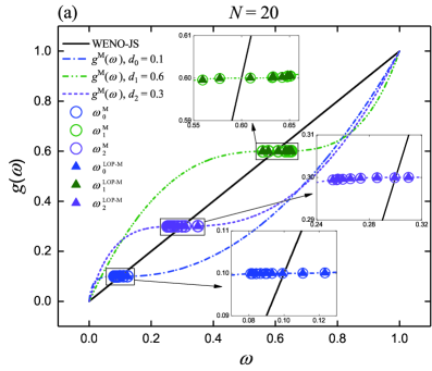
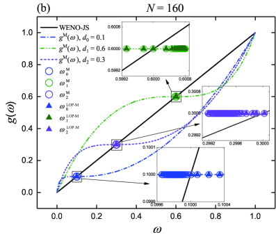
Fig. 1: Comparison for the real-time mappings on solving Eq.(12) with $u(x,0)=\sin(\pi x)$ using WENO-M and LOP-WENO-M.

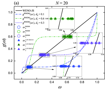
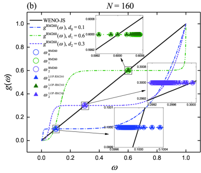
Fig. 2: Comparison for the real-time mappings on solving Eq.(12) with $u(x,0)=\sin(\pi x)$ using WENO-RM(260) and LOP-WENO-RM(260).

It is worthy to indicate that Lemma 4 is not always true when the initial condition includes discontinuities. To show this, we solve Eq.(12) with an initial condition as follows

$$\begin{array}[]{l}u(x,0)=\left\{\begin{array}[]{ll}\dfrac{1}{6}\big{[}G(x,\beta,z-\hat{\delta})+4G(x,\beta,z)+G(x,\beta,z+\hat{\delta})\big{]},&x\in[-0.8,-0.6],\\ 1,&x\in[-0.4,-0.2],\\ 1-\big{\lvert}10(x-0.1)\big{\rvert},&x\in[0.0,0.2],\\ \dfrac{1}{6}\big{[}F(x,\alpha,a-\hat{\delta})+4F(x,\alpha,a)+F(x,\alpha,a+\hat{\delta})\big{]},&x\in[0.4,0.6],\\ 0,&\mathrm{otherwise},\end{array}\right.\end{array}$$ (13)

where $G(x,\beta,z)=\mathrm{e}^{-\beta(x-z)^{2}},F(x,\alpha,a)=\sqrt{\max\big{(}1-\alpha^{2}(x-a)^{2},0\big{)}}$, and the constants are $z=-0.7,\hat{\delta}=0.005,\beta=\dfrac{\log 2}{36\hat{\delta}^{2}},a=0.5$ and $\alpha=10$. For brevity in the presentation, we call this Linear Problem SLP as it is presented by Shu et al. in [12]. It is known that this problem consists of a Gaussian, a square wave, a sharp triangle and a semi-ellipse. In the calculations here, the periodic boundary condition is used and the CFL number is taken to be $0.1$. We take a uniform cell number of $N=800$ and a short output time of $t=2$. In Fig. 3, we give the real-time mapping relationships of the LOP-WENO-X schemes, as well as the WENO-X schemes. It can be seen that the real-time mapping relationships of the LOP-WENO-X schemes are very different from those of the WENO-X schemes.

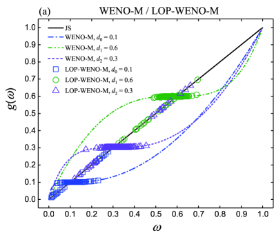
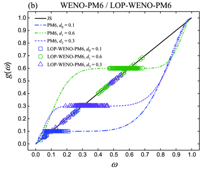
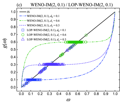
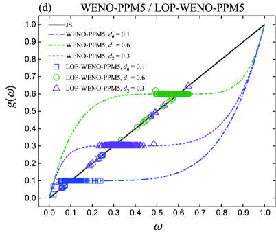
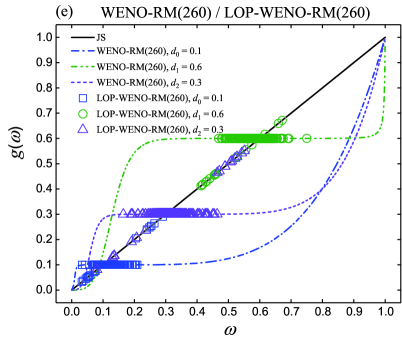
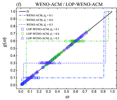
Fig. 3: Comparison for the real-time mappings on solving SLP using WENO-X and LOP-WENO-X.

In Theorem 3, we give the convergence properties of the $(2r-1)$th-order LOP-WENO-X schemes. As Theorem 2 is true, the proof of Theorem 3 is almost identical to that of the associated WENO-X schemes in the references presented in Table 1.

Theorem 3

The requirements for the $(2r-1)$th-order LOP-WENO-X schemes to achieve the optimal order of accuracy are identical to those of their associated $(2r-1)$th-order WENO-X scheme.

3.4 Long-run simulations of linear advection equation for comparison

3.4.1 With high-order critical points

In order to demonstrate the ability of the LOP-WENO-X schemes that they can preserve high resolutions for the problem including high-order critical points with long output times, we conduct the following test.

Example 1

We solve Eq.(12) with the periodic boundary condition by considering an initial condition that has high-order critical points, taking the form

$$u(x,0)=\exp\Big{(}-\big{(}x-9.0\big{)}^{5}\cos^{9}\big{(}\pi(x-9.0)\big{)}\Big{)},$$ (14)

In this test, the computational domain is $x\in(7.5,10.5)$ and the CFL number is $(\Delta x)^{2/3}$.

The following $L_{1}$ and $L_{\infty}$ errors are computed to test the dissipations of the schemes

$$L_{1}=h\cdot\sum\nolimits_{i=1}^{N}\Big{\lvert}u_{i}^{\mathrm{exact}}-(u_{h})_{i}\Big{\rvert},\quad L_{\infty}=\max_{1\leq i\leq N}\Big{\lvert}u_{i}^{\mathrm{exact}}-(u_{h})_{i}\Big{\rvert},$$ (15)

where $N$ is the number of the cells and $h$ is the associated uniform spatial step size. $(u_{h})_{i}$ is the numerical solution and $u_{i}^{\mathrm{exact}}$ is the exact solution. It is trivial to verify that the exact solution is $u(x,t)=\exp\Big{(}-\big{(}(x-t)-9.0\big{)}^{5}\cos^{9}\big{(}\pi((x-t)-9.0)\big{)}\Big{)}$.

In addition, the following increased errors are considered

$$\chi_{1}=\frac{L_{1}^{\mathrm{Y}}(t)-L_{1}^{\mathrm{ILW}}(t)}{L_{1}^{\mathrm{ILW}}(t)}\times 100\%,\quad\chi_{\infty}=\frac{L_{\infty}^{\mathrm{Y}}(t)-L_{\infty}^{\mathrm{ILW}}(t)}{L_{\infty}^{\mathrm{ILW}}(t)}\times 100\%,$$

where $L_{1}^{\mathrm{ILW}}(t)$ and $L_{\infty}^{\mathrm{ILW}}(t)$ are the $L_{1}$ and $L_{\infty}$ errors of the WENO5-ILW scheme (say, the WENO5 scheme using ideal linear weights), and similarly, $L_{1}^{\mathrm{Y}}(t)$ and $L_{\infty}^{\mathrm{Y}}(t)$ are those of the scheme “Y”.

Table 2: $L_{1}$, $L_{\infty}$ errors and the increased errors (in percentage) of various considered schemes on solving $u_{t}+u_{x}=0$ with initial condition Eq.(14) and $N=300$.

	WENO5-ILW				WENO-JS
Time, $t$	$L_{1}$ error	$\chi_{1}$	$L_{\infty}$ error	$\chi_{\infty}$	$L_{1}$ error	$\chi_{1}$	$L_{\infty}$ error	$\chi_{\infty}$
15	9.39243E-04	-	1.43469E-03	-	1.53437E-03	63%	2.70581E-03	89%
60	1.18694E-03	-	2.20682E-03	-	4.94939E-03	317%	8.38132E-03	280%
150	2.85184E-03	-	4.96667E-03	-	2.15858E-02	657%	5.25441E-02	958%
300	5.39974E-03	-	8.81363E-03	-	7.93589E-02	1370%	1.34321E-01	1424%
600	9.94133E-03	-	1.50917E-02	-	2.10016E-01	2013%	3.04860E-01	1920%
900	1.38061E-02	-	1.96281E-02	-	2.84632E-01	1962%	4.20080E-01	2040%
1200	1.74067E-02	-	2.39652E-02	-	3.26687E-01	1777%	5.14072E-01	2045%
	WENO-M				LOP-WENO-M
Time, $t$	$L_{1}$ error	$\chi_{1}$	$L_{\infty}$ error	$\chi_{\infty}$	$L_{1}$ error	$\chi_{1}$	$L_{\infty}$ error	$\chi_{\infty}$
15	9.63640E-04	3%	1.43486E-03	0%	1.12245E-03	20%	1.45965E-03	2%
60	1.59176E-03	34%	4.93572E-03	124%	3.13037E-03	164%	9.68122E-03	339%
150	6.91167E-03	142%	3.05991E-02	516%	9.04418E-03	217%	1.62967E-02	228%
300	3.02283E-02	460%	1.13618E-01	1189%	1.14248E-02	112%	1.86573E-02	112%
600	9.06252E-02	812%	1.76325E-01	1068%	2.28157E-02	130%	4.01795E-02	166%
900	1.52637E-01	1006%	3.25300E-01	1557%	2.84909E-02	106%	3.99876E-02	104%
1200	1.95044E-01	1021%	3.32396E-01	1287%	2.68748E-02	54%	3.08547E-02	29%
	WENO-PM6				LOP-WENO-PM6
Time, $t$	$L_{1}$ error	$\chi_{1}$	$L_{\infty}$ error	$\chi_{\infty}$	$L_{1}$ error	$\chi_{1}$	$L_{\infty}$ error	$\chi_{\infty}$
15	9.33637E-04	-1%	1.43467E-03	0%	1.11346E-03	19%	1.43572E-03	0%
60	1.13744E-03	-4%	2.20467E-03	0%	3.03330E-03	156%	9.06783E-03	311%
150	2.68760E-03	-6%	4.88656E-03	-2%	9.07249E-03	218%	1.65412E-02	233%
300	4.97186E-03	-8%	8.79888E-03	0%	1.09817E-02	103%	1.96942E-02	123%
600	8.51389E-03	-14%	1.49420E-02	-1%	1.89507E-02	91%	2.99502E-02	98%
900	1.12016E-02	-19%	1.90706E-02	-3%	2.55009E-02	85%	4.82978E-02	146%
1200	1.36304E-02	-22%	2.30084E-02	-4%	2.47046E-02	42%	3.57705E-02	49%
	WENO-IM(2, 0.1)				LOP-WENO-IM(2, 0.1)
Time, $t$	$L_{1}$ error	$\chi_{1}$	$L_{\infty}$ error	$\chi_{\infty}$	$L_{1}$ error	$\chi_{1}$	$L_{\infty}$ error	$\chi_{\infty}$
15	9.41045E-04	0%	1.43471E-03	0%	1.11781E-03	19%	1.76330E-03	23%
60	1.19465E-03	1%	2.21080E-03	0%	3.07175E-03	159%	9.21010E-03	317%
150	2.79176E-03	-2%	4.99982E-03	1%	9.02303E-03	216%	1.65281E-02	233%
300	5.09842E-03	-6%	8.83560E-03	0%	1.09585E-02	103%	1.88913E-02	114%
600	8.84945E-03	-11%	1.48704E-02	-1%	2.07426E-02	109%	3.28878E-02	118%
900	1.17416E-02	-15%	1.91100E-02	-3%	2.64361E-02	91%	4.61971E-02	135%
1200	1.43988E-02	-17%	2.31394E-02	-3%	2.54519E-02	46%	2.93893E-02	23%
	WENO-PPM5				LOP-WENO-PPM5
Time, $t$	$L_{1}$ error	$\chi_{1}$	$L_{\infty}$ error	$\chi_{\infty}$	$L_{1}$ error	$\chi_{1}$	$L_{\infty}$ error	$\chi_{\infty}$
15	9.34095E-04	-1%	1.43467E-03	0%	1.11267E-03	18%	1.43465E-03	0%
60	1.14062E-03	-4%	2.20440E-03	0%	3.02337E-03	155%	9.03860E-03	310%
150	2.69185E-03	-6%	4.89513E-03	-1%	9.07221E-03	218%	1.65292E-02	233%
300	4.98381E-03	-8%	8.79434E-03	0%	1.10228E-02	104%	2.01451E-02	129%
600	8.54488E-03	-14%	1.49710E-02	-1%	1.89501E-02	91%	2.96365E-02	96%
900	1.12525E-02	-18%	1.91124E-02	-3%	2.55066E-02	85%	4.90556E-02	150%
1200	1.37002E-02	-21%	2.30576E-02	-4%	2.48630E-02	43%	3.66520E-02	53%
	WENO-RM(260)				LOP-WENO-RM(260)
Time, $t$	$L_{1}$ error	$\chi_{1}$	$L_{\infty}$ error	$\chi_{\infty}$	$L_{1}$ error	$\chi_{1}$	$L_{\infty}$ error	$\chi_{\infty}$
15	9.39107E-04	0%	1.43469E-03	0%	1.11731E-03	19%	1.44384E-03	1%
60	1.16183E-03	-2%	2.20830E-03	0%	3.06524E-03	158%	9.17780E-03	316%
150	2.70494E-03	-5%	4.89842E-03	-1%	9.02171E-03	216%	1.65533E-02	233%
300	4.99464E-03	-8%	8.80531E-03	0%	1.09337E-02	102%	1.88283E-02	114%
600	8.56131E-03	-14%	1.49164E-02	-1%	2.03795E-02	105%	3.22925E-02	114%
900	1.12528E-02	-18%	1.90455E-02	-3%	2.62193E-02	90%	4.60197E-02	134%
1200	1.36724E-02	-21%	2.29797E-02	-4%	2.53001E-02	45%	2.94014E-02	23%
	WENO-ACM				LOP-WENO-ACM
Time, $t$	$L_{1}$ error	$\chi_{1}$	$L_{\infty}$ error	$\chi_{\infty}$	$L_{1}$ error	$\chi_{1}$	$L_{\infty}$ error	$\chi_{\infty}$
15	9.39110E-04	0%	1.43469E-03	0%	1.11724E-03	19%	1.44365E-03	1%
60	1.17055E-03	-1%	2.20771E-03	0%	3.06492E-03	158%	9.17648E-03	316%
150	2.70928E-03	-5%	4.92156E-03	-1%	9.02312E-03	216%	1.65537E-02	233%
300	5.02511E-03	-7%	8.79766E-03	0%	1.09333E-02	102%	1.88278E-02	114%
600	8.63079E-03	-13%	1.49585E-02	-1%	2.03612E-02	105%	3.22898E-02	114%
900	1.13152E-02	-18%	1.91098E-02	-3%	2.62113E-02	90%	4.59477E-02	134%
1200	1.37302E-02	-21%	2.30445E-02	-4%	2.53002E-02	45%	2.94013E-02	23%

In Table 2, we present the $L_{1}$ and $L_{\infty}$ errors and the increased errors with $N=300$ at various final times of $t=15,60,150,300,600,900,1200$. We can find that: (1) the WENO-JS scheme produces the largest $L_{1}$ and $L_{\infty}$ errors, leading to the largest increased errors, among all considered schemes for each output time; (2) when the output time is small, like $t\leq 60$, the WENO-M scheme provides more accurate results than the LOP-WENO-M scheme, leading to smaller increased errors; (3) however, when the output time gets larger, like $t\geq 300$, the increased errors of the LOP-WENO-M scheme evidently decrease and get closer to those of the WENO5-ILW scheme, while the errors of the WENO-M scheme increase significantly leading to extremely larger increased errors; (4) in spite that the errors of the LOP-WENO-X schemes (except the case of “X = M”) are larger than those of their associated WENO-X schemes, these errors can maintain a acceptable level leading to tolerable increased errors that are far lower than those of the WENO-JS and WENO-M schemes, and moreover, the LOP-WENO-X schemes are able to avoid the spurious oscillations on solving problems with discontinuities for long output times while their associated WENO-X schemes fail to prevent the spurious oscillations (for example, see Fig. 5 and Fig. 6).

Fig. 4 shows the performances of various considered schemes at output time $t=1200$ with the grid number of $N=300$. From Fig. 4, we can find that: (1) the WENO-JS scheme shows the lowest resolution, followed by the WENO-M scheme whose resolution is far lower than its associated LOP-WENO-M scheme; (2) the other LOP-WENO-X schemes give results with slightly lower resolutions than their associated WENO-X schemes but they still show far better resolutions than the WENO-M and WENO-JS schemes.

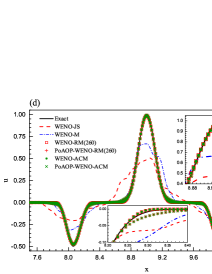
Fig. 4: Performance of various WENO schemes for Example 1 at output time $t=1200$ with $N=300$.

3.4.2 With discontinuities

To show the advantage of the LOP-WENO-X schemes that they can not only preserve high resolutions but also prevent spurious oscillations especially for long output time computations, we solve Eq.(12) with the periodic boundary condition by considering the following initial condition.

Example 2

The initial condition is given by

$$\begin{array}[]{l}u(x,0)=\left\{\begin{array}[]{ll}1.0,&x\in[-1.0,0.0],\\ 0.0,&x\in(0.0,1.0].\end{array}\right.\end{array}$$ (16)

It simply consists of two constant states separated by sharp discontinuities at $x=0.0,\pm 1.0$.

Firstly, we examine the convergence properties of the considered schemes with the output time $t=2000$. Here, the CFL number is taken to be $0.1$. For the purpose of comparison, we also present the results computed by the WENO5-ILW scheme.

We give the $L_{1}$, $L_{\infty}$ errors and the corresponding convergence orders in Table 3. We can see that: (1) the WENO-JS scheme produces significantly larger numerical errors than all other schemes and this indicates that it has the highest dissipation among all schemes; (2) the numerical errors generated by the LOP-WENO-M scheme are much smaller than its associated WENO-M scheme, especially for the $L_{1}$ errors for the computing cases of $N=400,800$, and this demonstrates the advantage of the LOP-WENO-M scheme of decreasing the dissipation; (3) the $L_{1}$ orders of the other mapped WENO-X schemes are clearly lower than those of their associated LOP-WENO-X schemes although their corresponding numerical errors are slightly smaller; (4) the $L_{\infty}$ errors of the LOP-WENO-X schemes are very close to, or even smaller for many cases than, their associated mapped WENO-X schemes. Moreover, if we take a view of the $x-u$ profiles, we can find that the resolution of the result computed by the WENO-M scheme is significantly lower than that of the LOP-WENO-M scheme, and the other mapped WENO-X schemes generate spurious oscillations but their associated LOP-WENO-X schemes do not. To manifest this, detailed tests will be conducted and the solutions will be presented carefully in the following pages.

Table 3: Numerical errors and convergence orders of accuracy on Example 16 at $t=2000.0$.

	WENO5-ILW				WENO-JS
$N$	$L_{1}$ error	$L_{1}$ order	$L_{\infty}$ error	$L_{\infty}$ order	$L_{1}$ error	$L_{1}$ order	$L_{\infty}$ error	$L_{\infty}$ order
200	1.03240E-01	-	4.67252E-01	-	4.48148E-01	-	5.55748E-01	-
400	5.79848E-02	0.8323	4.70837E-01	-0.0110	3.37220E-01	0.4103	5.77105E-01	-0.0544
800	3.25843E-02	0.8315	4.74042E-01	-0.0098	2.93752E-01	0.1991	5.17829E-01	0.1564
	WENO-M				LOP-WENO-M
$N$	$L_{1}$ error	$L_{1}$ order	$L_{\infty}$ error	$L_{\infty}$ order	$L_{1}$ error	$L_{1}$ order	$L_{\infty}$ error	$L_{\infty}$ order
200	1.76398E-01	-	5.27583E-01	-	1.22201E-01	-	5.04793E-01	-
400	1.67082E-01	0.0783	5.73328E-01	-0.1200	6.77592E-02	0.8508	4.88315E-01	0.0479
800	2.00760E-01	-0.2649	5.47150E-01	0.0674	3.67281E-02	0.8835	4.90550E-01	-0.0066
	WENO-PM6				LOP-WENO-PM6
$N$	$L_{1}$ error	$L_{1}$ order	$L_{\infty}$ error	$L_{\infty}$ order	$L_{1}$ error	$L_{1}$ order	$L_{\infty}$ error	$L_{\infty}$ order
200	8.67541E-02	-	5.02070E-01	-	1.19011E-01	-	4.75985E-01	-
400	5.29105E-02	0.7134	5.09366E-01	-0.0208	6.45626E-02	0.8823	4.95054E-01	-0.0567
800	2.97704E-02	0.8297	5.15102E-01	-0.0162	3.52222E-02	0.8742	4.75635E-01	0.0577
	WENO-IM(2, 0.1)				LOP-WENO-IM(2, 0.1)
$N$	$L_{1}$ error	$L_{1}$ order	$L_{\infty}$ error	$L_{\infty}$ order	$L_{1}$ error	$L_{1}$ order	$L_{\infty}$ error	$L_{\infty}$ order
200	7.94092E-02	-	4.64949E-01	-	1.22302E-01	-	5.08308E-01	-
400	4.61209E-02	0.7839	4.76074E-01	-0.0341	6.64627E-02	0.8798	5.02003E-01	0.0180
800	2.65533E-02	0.7965	4.91316E-01	-0.0455	3.61408E-02	0.8789	4.79591E-01	0.0659
	WENO-PPM5				LOP-WENO-PPM5
$N$	$L_{1}$ error	$L_{1}$ order	$L_{\infty}$ error	$L_{\infty}$ order	$L_{1}$ error	$L_{1}$ order	$L_{\infty}$ error	$L_{\infty}$ order
200	9.20390E-02	-	4.99999E-01	-	1.17886E-01	-	4.84251E-01	-
400	5.27679E-02	0.8026	5.07952E-01	-0.0228	6.58012E-02	0.8412	5.04572E-01	-0.0593
800	2.96879E-02	0.8298	5.14059E-01	-0.0172	3.58152E-02	0.8775	4.99765E-01	0.0138
	WENO-RM(260)				LOP-WENO-RM(260)
$N$	$L_{1}$ error	$L_{1}$ order	$L_{\infty}$ error	$L_{\infty}$ order	$L_{1}$ error	$L_{1}$ order	$L_{\infty}$ error	$L_{\infty}$ order
200	8.64542E-02	-	5.02486E-01	-	1.19069E-01	-	5.09991E-01	-
400	5.17965E-02	0.7391	5.08770E-01	-0.0179	6.58446E-02	0.8547	5.02010E-01	0.0228
800	2.91482E-02	0.8294	5.14009E-01	-0.0148	3.63654E-02	0.8565	4.78897E-01	0.0680
	WENO-ACM				LOP-WENO-ACM
$N$	$L_{1}$ error	$L_{1}$ order	$L_{\infty}$ error	$L_{\infty}$ order	$L_{1}$ error	$L_{1}$ order	$L_{\infty}$ error	$L_{\infty}$ order
200	8.87640E-02	-	5.06230E-01	-	1.21982E-01	-	5.14204E-01	-
400	5.16217E-02	0.7820	5.11512E-01	-0.0150	6.55457E-02	0.8961	4.98088E-01	0.0459
800	2.94211E-02	0.8111	5.15990E-01	-0.0126	3.61428E-02	0.8588	4.79224E-01	0.0557

To provide a better illustration, we re-calculate Example 16 by considered WENO schemes with the output time $t=200$ using the uniform meshes of $N=1600$ and $N=3200$, respectively.

Fig. 5 shows the comparison of considered schemes with $t=200$ and $N=1600$. We can observe that: (1) all the LOP-WENO-X schemes provide the numerical results with significantly higher resolutions than those of the WENO-JS and WENO-M schemes, and moreover, they are all able to avoid the spurious oscillations that will be inevitably generated by most of their associated mapped WENO-X schemes; (2) it seems that the WENO-IM(2, 0.1) scheme almost does not generate spurious oscillations and it gains better resolutions than the LOP-WENO-IM(2, 0.1) scheme in most of the region; (3) however, if we take a closer look, we can see that the WENO-IM(2, 0.1) scheme also generates very slight spurious oscillations as shown in Fig. 5(b-2).

The comparison of considered schemes for the case of $t=200$ and $N=3200$ are shown in Fig. 6. We can find that: (1) as the grid number increases, the spurious oscillations produced by the WENO-IM(2, 0.1) scheme become more violent and they are easily to be observed, however, the LOP-WENO-IM(2, 0.1) scheme can still prevent the spurious oscillations but provide very high resolutions; (2) all the LOP-WENO-X schemes still evidently provide much better resolutions than those of the WENO-JS and WENO-M schemes; (3) as the grid number increases, the spurious oscillations generated by the WENO-X schemes appear to be closer to the discontinuities, and the amplitudes of these spurious oscillations become larger; (4) furthermore, even though the grid number increases, the LOP-WENO-X schemes can still avoid spurious oscillations but obtain the great improvement of the resolution.

Taken together, the results above suggest that the LOP property, satisfied by the posteriori adaptive OP mapping in the present study, can help to preserve high resolutions and meanwhile avoid spurious oscillations in the simulation of problems with discontinuities, especially for long output times. And this is a very important aspect of this paper.

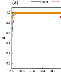
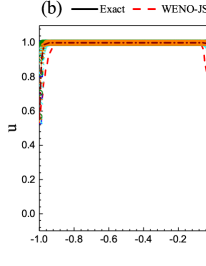
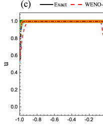
Fig. 5: Performance of the considered WENO schemes for Example 16 at output time $t=200$ with $N=1600$.

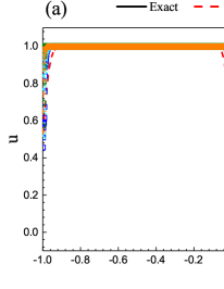
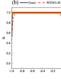
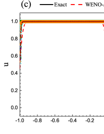
Fig. 6: Performance of the considered WENO schemes for Example 16 at output time $t=200$ with $N=3200$.

4 Numerical experiments for Euler equations

In this section, we apply the various considered schemes to solve the Euler equations. In all calculations, we choose $\epsilon$ in Eq.(6) to be $10^{-40}$ as recommended in [11, 4]. The local characteristic decomposition [12] is used when the WENO schemes are applied to solve the Euler system.

4.1 Comparisons of the performances on simulating problems with high-frequency smooth waves

In this subsection, we compare the numerical results of the LOP-WENO-X schemes with those of the MOP-WENO-X, WENO-X and WENO-JS schemes on calculating problems with high-frequency smooth waves. The considered problems are governed by the following one-dimensional Euler systems of compressible gas dynamics

$$\dfrac{\partial\mathbf{U}}{\partial t}+\dfrac{\partial\mathbf{F(U)}}{\partial x}=\mathbf{0},$$ (17)

with

$$\begin{array}[]{l}\mathbf{U}=\Big{(}\rho,\rho u,E\Big{)}^{\mathrm{T}},\quad\mathbf{F(U)}=\Big{(}\rho u,\rho u^{2}+p,u(E+p)\Big{)}^{\mathrm{T}},\end{array}$$

where $\rho,u,p$ and $E$ are the density, velocity in the $x$ coordinate direction, pressure and total energy, respectively. The relation of pressure $p$ and total energy for ideal gases is defined by

$$p=(\gamma-1)\Big{(}E-\dfrac{1}{2}\rho u^{2}\Big{)},\quad\gamma=1.4.$$

4.1.1 Shu-Osher problem

Example 3

This problem was presented by Shu and Osher [24]. The computational domain of $[-5,5]$ is initialized by

$$\big{(}\rho,u,p\big{)}(x,0)=\left\{\begin{array}[]{ll}(3.857143,2.629369,10.333333),&x\in[-5.0,-4.0],\\ (1.0+0.2\sin(5x),0,1),&x\in[-4.0,5.0].\end{array}\right.$$ (18)

The transmissive boundary conditions are used at $x=\pm 5$, and the output time is set to be $t=1.8$.

We compute this problem with a uniform cell number of $N=300$ by setting the CFL number to be 0.1. The solutions of density are given in Fig. 7 to Fig. 12 where the reference solution is computed by employing WENO-JS with $N=10000$. For comparison purpose, we also present the solutions of the associated MOP-WENO-X schemes proposed in our previous work [18] and that of WENO-JS. Obviously, WENO-JS provides the lowest resolution. Unfortunately, the resolutions of the MOP-WENO-X schemes are much lower than those of the WENO-X schemes. However, the LOP-WENO-X schemes can get comparable resolutions with those of the WENO-X schemes.

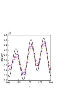
Fig. 7: Results of LOP-/MOP-/WENO-M and WENO-JS on solving the Shu-Osher problem.

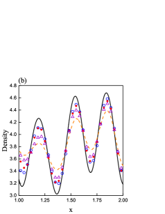
Fig. 9: Results of LOP-/MOP-/WENO-IM(2, 0.1) and WENO-JS on solving the Shu-Osher problem.

Fig. 10: Results of LOP-/MOP-/WENO-PPM5 and WENO-JS on solving the Shu-Osher problem.

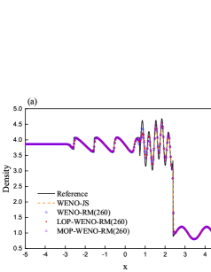
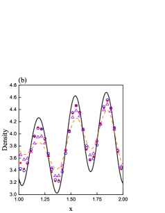
Fig. 11: Results of LOP-/MOP-/WENO-RM(260) and WENO-JS on solving the Shu-Osher problem.

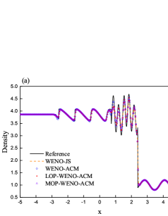
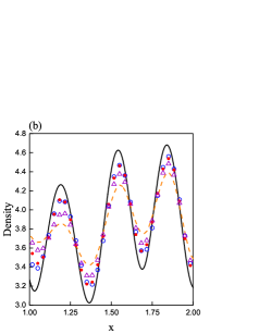
Fig. 12: Results of LOP-/MOP-/WENO-ACM and WENO-JS on solving the Shu-Osher problem.

4.1.2 Titarev-Toro problem

Example 4

This problem was presented by Titarev and Toro [25, 27, 26] and it is a more severe version of the Shu-Osher problem. The computational domain of $[-5,5]$ is initialized by

$$\big{(}\rho,u,p\big{)}(x,0)=\left\{\begin{array}[]{ll}(1.515695,0.5233346,1.80500),&x\in[-5.0,-4.5],\\ (1.0+0.1\sin(20\pi x),0,1),&x\in[-4.5,5.0].\end{array}\right.$$ (19)

Also, the transmissive boundary conditions are used at $x=\pm 5$, while the output time is set to be $t=5.0$ in this case.

We compute this problem with a uniform cell number of $N=1500$ by setting the CFL number to be 0.4. The solutions of density are given in Fig. 13 to Fig. 18 where the reference solution is computed by employing WENO-JS with $N=10000$. Again, for comparison purpose, we show the solutions of the associated MOP-WENO-X schemes and that of WENO-JS. Not surprisingly, WENO-JS provides the lowest resolution and the resolutions of the MOP-WENO-X schemes are much lower than those of the WENO-X schemes. Particularly, the resolutions of the LOP-WENO-X schemes are significantly higher than those of the WENO-X schemes. This is a remarkable competitive advantage of the LOP-WENO-X schemes compared to the MOP-WENO-X schemes.

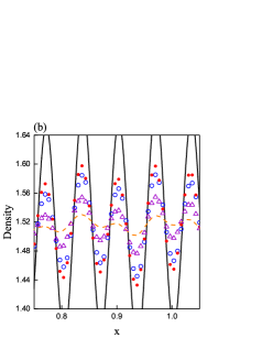
Fig. 13: Results of LOP-/MOP-/WENO-M and WENO-JS on solving the Titarev-Toro problem.

Fig. 14: Results of LOP-/MOP-/WENO-PM6 and WENO-JS on solving the Titarev-Toro problem.

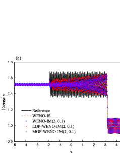
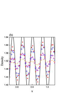
Fig. 15: Results of LOP-/MOP-/WENO-IM(2, 0.1) and WENO-JS on solving the Titarev-Toro problem.

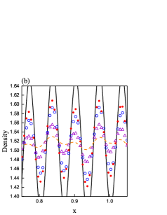
Fig. 16: Results of LOP-/MOP-/WENO-PPM5 and WENO-JS on solving the Titarev-Toro problem.

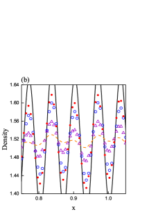
Fig. 17: Results of LOP-/MOP-/WENO-RM(260) and WENO-JS on solving the Titarev-Toro problem.

Fig. 18: Results of LOP-/MOP-/WENO-ACM and WENO-JS on solving the Titarev-Toro problem.

4.2 2D Euler equations

In this subsection, we consider the following two-dimensional Euler systems of compressible gas dynamics

$$\dfrac{\partial\mathbf{U}}{\partial t}+\dfrac{\partial\mathbf{F(U)}}{\partial x}+\dfrac{\partial\mathbf{G(U)}}{\partial y}=\mathbf{0},$$ (20)

with

$$\begin{array}[]{l}\mathbf{U}=\Big{(}\rho,\rho u,\rho v,E\Big{)}^{\mathrm{T}},\\ \mathbf{F(U)}=\Big{(}\rho u,\rho u^{2}+p,\rho uv,u(E+p)\Big{)}^{\mathrm{T}},\\ \mathbf{G(U)}=\Big{(}\rho v,\rho vu,\rho v^{2}+p,v(E+p)\Big{)}^{\mathrm{T}},\end{array}$$

where $\rho,u,v,p$ and $E$ are the density, components of velocity in the $x$ and $y$ coordinate directions, pressure and total energy, respectively. The relation of pressure $p$ and total energy for ideal gases is defined by

$$p=(\gamma-1)\Big{(}E-\dfrac{1}{2}\rho(u^{2}+v^{2})\Big{)},\quad\gamma=1.4.$$

Two commonly used classes of finite volume WENO schemes in two-dimensional Cartesian meshes were studied carefully by Zhang et al. [29]. Here, we implement the one denoted as class A for our calculations. Now, we examine the performances of the considered WENO shcemes on solving the following three benchmark tests.

4.2.1 Accuracy test 1

Example 5

We use this density wave propagation problem [13] to test the convergence orders of the considered WENO schemes. The initial condition on the computational domain $[-1.0,1.0]\times[-1.0,1.0]$ is given by

$$(\rho,u,v,p)(x,y,0)=\Big{(}1.0+0.2\sin\big{(}\pi(x+y)\big{)},0.7,0.3,1.0\Big{)}.$$ (21)

Here, the $L_{1}$ and $L_{\infty}$ errors are computed by

$$L_{1}=h_{x}h_{y}\cdot\sum\nolimits_{j=1}^{N_{y}}\sum\nolimits_{i=1}^{N_{x}}\Big{\lvert}\rho_{i,j}^{\mathrm{exact}}-(\rho_{h})_{i,j}\Big{\rvert},\quad L_{\infty}=\max_{\begin{subarray}{c}1\leq i\leq N_{x}\\ 1\leq j\leq N_{y}\end{subarray}}\Big{\lvert}\rho_{i,j}^{\mathrm{exact}}-(\rho_{h})_{i,j}\Big{\rvert},$$

where $N_{x},N_{y}$ is the number of cells in $x-$ and $y-$ direction, and $h_{x},h_{y}$ is the associated uniform spatial step size and we set $h=h_{x}=h_{y}$ in all calculations of this paper. $(\rho_{h})_{i,j}$ is the numerical solution of the density and $\rho_{i,j}^{\mathrm{exact}}$ is its exact solution. We can easily check that the exact solution is $\rho(x,y,t)=1.0+0.2\sin\Big{(}\pi\big{(}x+y-(u+v)t\big{)}\Big{)}$, $u(x,y,t)=0.7$ , $v(x,y,t)=0.3$, and $p(x,y,t)=1.0$.

The computational time is advanced until $t=2.0$. The periodic boundary condition is used and the CFL number is taken to be $h^{2/3}$ so that the error for the overall scheme is a measure of the spatial convergence only.

The numerical errors and corresponding convergence orders of accuracy for the density $\rho$ are shown in Table 4. Again, for comparison purpose, we also present the results computed by the WENO5-ILW scheme. We can see that all the considered WENO schemes can achieve the disgned order of accuracy, while the error magnitude is larger for the WENO-JS scheme than for the other schemes. Moreover, as expected, the numerical errors with respect to all grid numbers of the LOP-WENO-X schemes are almost the same to those of the WENO-X schemes. It should be noted that, in terms of accuracy, the LOP-WENO-PM6, LOP-WENO-PPM5, LOP-WENO-RM(260) and LOP-WENO-ACM schemes provide the numerical errors equivalent to that of the WENO5-ILW scheme, but of course this is not always the case and we will show it in the next test.

Table 4: Numerical errors and convergence orders of accuracy for the density $\rho$ on Example 5 at $t=2.0$.

	WENO5-ILW				WENO-JS
$N_{x}\times N_{y}$	$L_{1}$ error	$L_{1}$ order	$L_{\infty}$ error	$L_{\infty}$ order	$L_{1}$ error	$L_{1}$ order	$L_{\infty}$ error	$L_{\infty}$ order
40 $\times$ 40	2.05111E-05	-	8.06075E-06	-	1.44379E-04	-	6.11870E-05	-
60 $\times$ 60	2.71152E-06	4.9905	1.06517E-06	4.9915	1.90416E-05	4.9963	8.53414E-06	4.8583
80 $\times$ 80	6.44325E-07	4.9953	2.53073E-07	4.9958	4.51609E-06	5.0020	2.03906E-06	4.9763
100 $\times$ 100	2.11264E-07	4.9972	8.29736E-08	4.9975	1.47974E-06	5.0003	6.75061E-07	4.9539
	WENO-M				LOP-WENO-M
$N_{x}\times N_{y}$	$L_{1}$ error	$L_{1}$ order	$L_{\infty}$ error	$L_{\infty}$ order	$L_{1}$ error	$L_{1}$ order	$L_{\infty}$ error	$L_{\infty}$ order
40 $\times$ 40	2.05584E-05	-	8.07114E-06	-	2.05584E-05	-	8.07114E-06	-
60 $\times$ 60	2.71274E-06	4.9950	1.06546E-06	4.9940	2.71274E-06	4.9950	1.06546E-06	4.9940
80 $\times$ 80	6.44416E-07	4.9964	2.53097E-07	4.9965	6.44416E-07	4.9964	2.53097E-07	4.9965
100 $\times$ 100	2.11276E-07	4.9976	8.29769E-08	4.9977	2.11276E-07	4.9976	8.29769E-08	4.9977
	WENO-PM6				LOP-WENO-PM6
$N_{x}\times N_{y}$	$L_{1}$ error	$L_{1}$ order	$L_{\infty}$ error	$L_{\infty}$ order	$L_{1}$ error	$L_{1}$ order	$L_{\infty}$ error	$L_{\infty}$ order
40 $\times$ 40	2.05111E-05	-	8.06076E-06	-	2.05111E-05	-	8.06076E-06	-
60 $\times$ 60	2.71152E-06	4.9905	1.06517E-06	4.9915	2.71152E-06	4.9905	1.06517E-06	4.9915
80 $\times$ 80	6.44325E-07	4.9953	2.53073E-07	4.9958	6.44325E-07	4.9953	2.53073E-07	4.9958
100 $\times$ 100	2.11264E-07	4.9972	8.29736E-08	4.9975	2.11264E-07	4.9972	8.29736E-08	4.9975
	WENO-IM(2, 0.1)				LOP-WENO-IM(2, 0.1)
$N_{x}\times N_{y}$	$L_{1}$ error	$L_{1}$ order	$L_{\infty}$ error	$L_{\infty}$ order	$L_{1}$ error	$L_{1}$ order	$L_{\infty}$ error	$L_{\infty}$ order
40 $\times$ 40	2.05159E-05	-	8.06179E-06	-	2.05159E-05	-	8.06179E-06	-
60 $\times$ 60	2.71164E-06	4.9909	1.06520E-06	4.9917	2.71164E-06	4.9909	1.06520E-06	4.9917
80 $\times$ 80	6.44334E-07	4.9954	2.53076E-07	4.9959	6.44334E-07	4.9954	2.53076E-07	4.9959
100 $\times$ 100	2.11265E-07	4.9972	8.29739E-08	4.9975	2.11265E-07	4.9972	8.29739E-08	4.9975
	WENO-PPM5				LOP-WENO-PPM5
$N_{x}\times N_{y}$	$L_{1}$ error	$L_{1}$ order	$L_{\infty}$ error	$L_{\infty}$ order	$L_{1}$ error	$L_{1}$ order	$L_{\infty}$ error	$L_{\infty}$ order
40 $\times$ 40	2.05111E-05	-	8.06083E-06	-	2.05111E-05	-	8.06083E-06	-
60 $\times$ 60	2.71152E-06	4.9905	1.06517E-06	4.9915	2.71152E-06	4.9905	1.06517E-06	4.9915
80 $\times$ 80	6.44325E-07	4.9953	2.53073E-07	4.9958	6.44325E-07	4.9953	2.53073E-07	4.9958
100 $\times$ 100	2.11264E-07	4.9972	8.29736E-08	4.9975	2.11264E-07	4.9972	8.29736E-08	4.9975
	WENO-RM(260)				LOP-WENO-RM(260)
$N_{x}\times N_{y}$	$L_{1}$ error	$L_{1}$ order	$L_{\infty}$ error	$L_{\infty}$ order	$L_{1}$ error	$L_{1}$ order	$L_{\infty}$ error	$L_{\infty}$ order
40 $\times$ 40	2.05111E-05	-	8.06075E-06	-	2.05111E-05	-	8.06075E-06	-
60 $\times$ 60	2.71152E-06	4.9905	1.06517E-06	4.9915	2.71152E-06	4.9905	1.06517E-06	4.9915
80 $\times$ 80	6.44325E-07	4.9953	2.53073E-07	4.9958	6.44325E-07	4.9953	2.53073E-07	4.9958
100 $\times$ 100	2.11264E-07	4.9972	8.29736E-08	4.9975	2.11264E-07	4.9972	8.29736E-08	4.9975
	WENO-ACM				LOP-WENO-ACM
$N_{x}\times N_{y}$	$L_{1}$ error	$L_{1}$ order	$L_{\infty}$ error	$L_{\infty}$ order	$L_{1}$ error	$L_{1}$ order	$L_{\infty}$ error	$L_{\infty}$ order
40 $\times$ 40	2.05111E-05	-	8.06075E-06	-	2.05111E-05	-	8.06075E-06	-
60 $\times$ 60	2.71152E-06	4.9905	1.06517E-06	4.9915	2.71152E-06	4.9905	1.06517E-06	4.9915
80 $\times$ 80	6.44325E-07	4.9953	2.53073E-07	4.9958	6.44325E-07	4.9953	2.53073E-07	4.9958
100 $\times$ 100	2.11264E-07	4.9972	8.29736E-08	4.9975	2.11264E-07	4.9972	8.29736E-08	4.9975

4.2.2 Accuracy test 2

Example 6

Now we use a modified version of the density wave propagation problem [13] to test the convergence orders of the considered WENO schemes. Here, the initial condition on the computational domain $[-1.0,1.0]\times[-1.0,1.0]$ is given by

$$(\rho,u,v,p)(x,y,0)=\Bigg{(}1.0+0.2\sin\bigg{(}\pi(x+y)-\dfrac{\sin(\pi(x+y))}{\pi}\bigg{)},0.7,0.3,1.0\Bigg{)}.$$ (22)

Again, the computational time is advanced until $t=2.0$. And also the periodic boundary condition is used and the CFL number is taken to be $h^{2/3}$. Trivially, the exact solution is $\rho(x,y,t)=1.0+0.2\sin\Bigg{(}\pi\bigg{(}x+y-(u+v)t-\frac{\sin\Big{(}\pi\big{(}x+y-(u+v)t\big{)}\Big{)}}{\pi}\bigg{)}\Bigg{)}$, $u(x,y,t)=0.7$, $v(x,y,t)=0.3$, and $p(x,y,t)=1.0$.

The numerical errors and corresponding convergence orders of accuracy for the density $\rho$ are shown in Table 5. It is noted that the $L_{\infty}$ convergence order of the WENO-JS scheme drops by nearly 2 orders that leads to an overall accuracy loss shown with the $L_{1}$ convergence order. However, it is evident that the other schemes can retain the optimal convergence orders even in the presence of critical points. Unsurprisingly, in terms of accuracy, the LOP-WENO-X schemes give equally accurate numerical solutions like those of their associated WENO-X schemes. We point out that, for this test, only the LOP-WENO-ACM/WENO-ACM scheme provides the numerical errors equivalent to that of the WENO5-ILW scheme.

Table 5: Numerical errors and convergence orders of accuracy for the density $\rho$ on Example 6 at $t=2.0$.

	WENO5-ILW				WENO-JS
$N_{x}\times N_{y}$	$L_{1}$ error	$L_{1}$ order	$L_{\infty}$ error	$L_{\infty}$ order	$L_{1}$ error	$L_{1}$ order	$L_{\infty}$ error	$L_{\infty}$ order
40 $\times$ 40	2.31214E-04	-	1.58230E-04	-	8.15797E-04	-	5.48728E-04	-
60 $\times$ 60	3.13106E-05	4.9311	2.18798E-05	4.8795	1.61432E-04	3.9956	1.32554E-04	3.5037
80 $\times$ 80	7.48937E-06	4.9724	5.24972E-06	4.9617	4.67993E-05	4.3041	4.84021E-05	3.5019
100 $\times$ 100	2.46221E-06	4.9852	1.72697E-06	4.9825	1.76222E-05	4.3770	2.23573E-05	3.4614
	WENO-M				LOP-WENO-M
$N_{x}\times N_{y}$	$L_{1}$ error	$L_{1}$ order	$L_{\infty}$ error	$L_{\infty}$ order	$L_{1}$ error	$L_{1}$ order	$L_{\infty}$ error	$L_{\infty}$ order
40 $\times$ 40	2.21884E-04	-	1.57466E-04	-	2.21884E-04	-	1.57466E-04	-
60 $\times$ 60	3.06949E-05	4.8785	2.20005E-05	4.8540	3.06949E-05	4.8785	2.20005E-05	4.8540
80 $\times$ 80	7.40640E-06	4.9421	5.25840E-06	4.9751	7.40640E-06	4.9421	5.25840E-06	4.9751
100 $\times$ 100	2.44462E-06	4.9675	1.72528E-06	4.9943	2.44462E-06	4.9675	1.72528E-06	4.9943
	WENO-PM6				LOP-WENO-PM6
$N_{x}\times N_{y}$	$L_{1}$ error	$L_{1}$ order	$L_{\infty}$ error	$L_{\infty}$ order	$L_{1}$ error	$L_{1}$ order	$L_{\infty}$ error	$L_{\infty}$ order
40 $\times$ 40	2.35238E-04	-	1.57970E-04	-	2.35238E-04	-	1.57970E-04	-
60 $\times$ 60	3.14340E-05	4.9639	2.18667E-05	4.8770	3.14340E-05	4.9639	2.18667E-05	4.8770
80 $\times$ 80	7.49935E-06	4.9814	5.25053E-06	4.9591	7.49935E-06	4.9814	5.25053E-06	4.9591
100 $\times$ 100	2.46354E-06	4.9888	1.72711E-06	4.9828	2.46354E-06	4.9888	1.72711E-06	4.9828
	WENO-IM(2, 0.1)				LOP-WENO-IM(2, 0.1)
$N_{x}\times N_{y}$	$L_{1}$ error	$L_{1}$ order	$L_{\infty}$ error	$L_{\infty}$ order	$L_{1}$ error	$L_{1}$ order	$L_{\infty}$ error	$L_{\infty}$ order
40 $\times$ 40	2.30237E-04	-	1.57910E-04	-	2.30237E-04	-	1.57910E-04	-
60 $\times$ 60	3.12478E-05	4.9256	2.18921E-05	4.8732	3.12478E-05	4.9256	2.18921E-05	4.8732
80 $\times$ 80	7.48097E-06	4.9693	5.25058E-06	4.9631	7.48097E-06	4.9693	5.25058E-06	4.9631
100 $\times$ 100	2.46044E-06	4.9834	1.72680E-06	4.9836	2.46044E-06	4.9834	1.72680E-06	4.9836
	WENO-PPM5				LOP-WENO-PPM5
$N_{x}\times N_{y}$	$L_{1}$ error	$L_{1}$ order	$L_{\infty}$ error	$L_{\infty}$ order	$L_{1}$ error	$L_{1}$ order	$L_{\infty}$ error	$L_{\infty}$ order
40 $\times$ 40	2.35717E-04	-	1.57956E-04	-	2.35717E-04	-	1.57956E-04	-
60 $\times$ 60	3.15372E-05	4.9609	2.18541E-05	4.8782	3.15372E-05	4.9609	2.18541E-05	4.8782
80 $\times$ 80	7.51693E-06	4.9847	5.25176E-06	4.9563	7.51693E-06	4.9847	5.25176E-06	4.9563
100 $\times$ 100	2.46739E-06	4.9923	1.72749E-06	4.9829	2.46739E-06	4.9923	1.72749E-06	4.9829
	WENO-RM(260)				LOP-WENO-RM(260)
$N_{x}\times N_{y}$	$L_{1}$ error	$L_{1}$ order	$L_{\infty}$ error	$L_{\infty}$ order	$L_{1}$ error	$L_{1}$ order	$L_{\infty}$ error	$L_{\infty}$ order
40 $\times$ 40	2.31192E-04	-	1.58226E-04	-	2.31192E-04	-	1.58226E-04	-
60 $\times$ 60	3.13103E-05	4.9309	2.18799E-05	4.8795	3.13103E-05	4.9309	2.18799E-05	4.8795
80 $\times$ 80	7.48936E-06	4.9724	5.24972E-06	4.9617	7.48936E-06	4.9724	5.24972E-06	4.9617
100 $\times$ 100	2.46221E-06	4.9852	1.72697E-06	4.9825	2.46221E-06	4.9852	1.72697E-06	4.9825
	WENO-ACM				LOP-WENO-ACM
$N_{x}\times N_{y}$	$L_{1}$ error	$L_{1}$ order	$L_{\infty}$ error	$L_{\infty}$ order	$L_{1}$ error	$L_{1}$ order	$L_{\infty}$ error	$L_{\infty}$ order
40 $\times$ 40	2.31214E-04	-	1.58230E-04	-	2.31214E-04	-	1.58230E-04	-
60 $\times$ 60	3.13106E-05	4.9311	2.18798E-05	4.8795	3.13106E-05	4.9311	2.18798E-05	4.8795
80 $\times$ 80	7.48937E-06	4.9724	5.24972E-06	4.9617	7.48937E-06	4.9724	5.24972E-06	4.9617
100 $\times$ 100	2.46221E-06	4.9852	1.72697E-06	4.9825	2.46221E-06	4.9852	1.72697E-06	4.9825

4.2.3 Shock-vortex interaction problem

Example 7

The shock-vortex interaction problem is a very favorable 2D test case for high-resolution schemes [2, 20, 21]. The initial condition is given by

$$\big{(}\rho,u,v,p\big{)}(x,y,0)=\left\{\begin{aligned} \begin{array}[]{ll}(1,\sqrt{\gamma},0,1),&x<0.5,\\ \Bigg{(}\rho_{\mathrm{L}}\bigg{(}\dfrac{\gamma-1+(\gamma+1)p_{\mathrm{R}}}{\gamma+1+(\gamma-1)p_{\mathrm{R}}}\bigg{)},u_{\mathrm{L}}\bigg{(}\dfrac{1-p_{\mathrm{R}}}{\sqrt{\gamma-1+p_{\mathrm{R}}(\gamma+1)}}\bigg{)},0,1.3\Bigg{)},&x\geq 0.5.\\ \end{array}\end{aligned}\right.$$

The following perturbations is superimposed onto the left state,

$$\delta\rho=\dfrac{\rho_{\mathrm{L}}^{2}}{(\gamma-1)p_{\mathrm{L}}}\delta T,\delta u=\epsilon\dfrac{y-y_{\mathrm{c}}}{r_{\mathrm{c}}}\mathrm{e}^{\alpha(1-r^{2})},\delta v=-\epsilon\dfrac{x-x_{\mathrm{c}}}{r_{\mathrm{c}}}\mathrm{e}^{\alpha(1-r^{2})},\delta p=\dfrac{\gamma\rho_{\mathrm{L}}^{2}}{(\gamma-1)\rho_{\mathrm{L}}}\delta T,$$

where $\epsilon=0.3,r_{\mathrm{c}}=0.05,\alpha=0.204,x_{\mathrm{c}}=0.25,y_{\mathrm{c}}=0.5,r=\sqrt{((x-x_{\mathrm{c}})^{2}+(y-y_{\mathrm{c}})^{2})/r_{\mathrm{c}}^{2}},\delta T=-(\gamma-1)\epsilon^{2}\mathrm{e}^{2\alpha(1-r^{2})}/(4\alpha\gamma)$. The transmissive boundary condition is used. We compute the solution up to two different output times $t=0.35,0.60$ by using all considered schemes with a uniform mesh size of $800\times 800$. Here, we set the CFL number to be $0.5$.

Just for the sake of simplicity in presentation, we only show the density profiles of the WENO-M, WENO-PM6, WENO-IM(2, 0.1) schemes for $t=0.35$ (see Fig. 19), and the density profiles of the WENO-PPM5, WENO-RM(260), WENO-ACM schemes for $t=0.6$ (see Fig. 21). To unveil the advantage of the LOP-WENO-X schemes more precisely, we present the cross-sectional slices of density plots along the plane $y=0.65,0.75$ (see Fig. 20) and $y=0.25,0.3$ (see Fig. 22) of all considered schemes for $t=0.35$ and $t=0.6$, respectively. It can be seen that: (1) the main structure of the shock and vortex after the interaction were captured properly by all the considered schemes; (2) in the solutions of the WENO-X schemes, clear post-shock oscillations can be observed, whereas the post-shock oscillations are considerably reduced in the solutions of the associated LOP-WENO-X schemes; (3) it is easy to find that the amplitudes of the post-shock oscillations produced by the WENO-X schemes are much greater than those of their associated LOP-WENO-X schemes. In a word, the LOP-WENO-X schemes only produce some highly tolerable post-shock oscillations. This should be another merit of the mapped WENO schemes with LOP mappings.

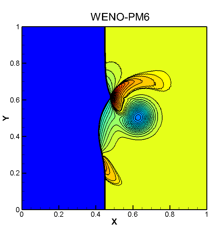
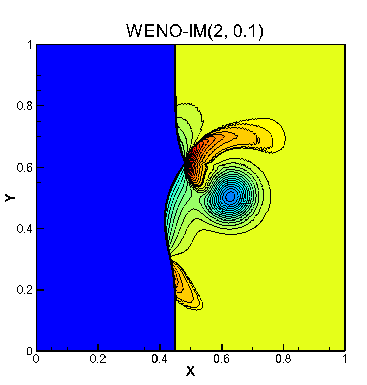
Fig. 19: Density plots for the Shock-vortex interaction, $t=0.35$.

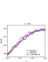
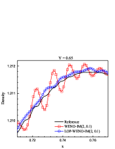
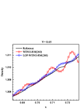
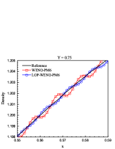
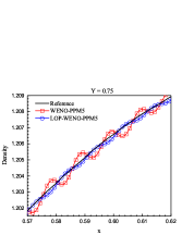
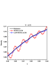
Fig. 20: Density cross-sectional slices plotted along the plane $y=0.65,0.75$ with $t=0.35$.

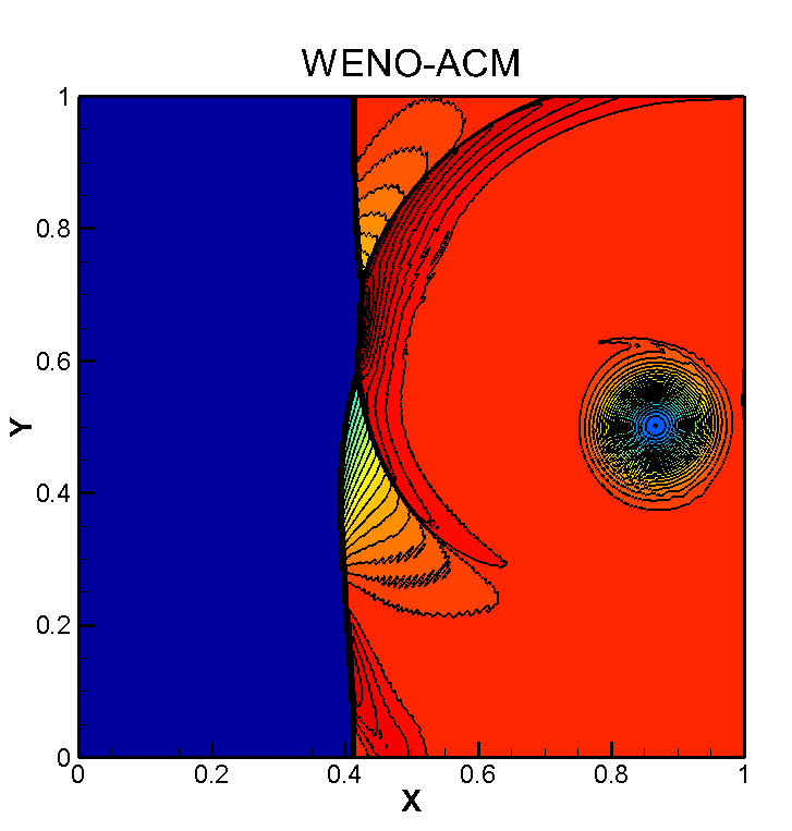
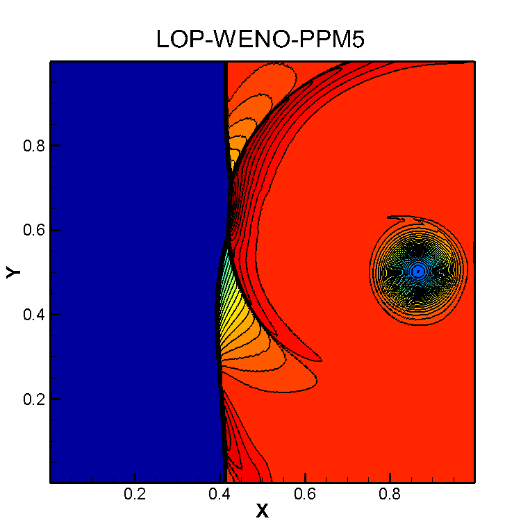
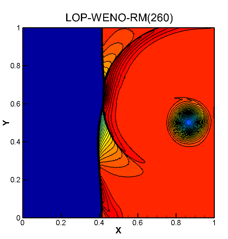
Fig. 21: Density plots for the Shock-vortex interaction, $t=0.6$.

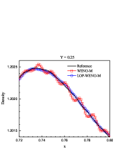
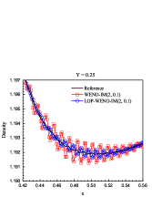
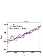
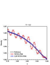
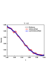
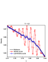
Fig. 22: Density cross-sectional slices plotted along the plane $y=0.25,0.30$ with $t=0.60$.

5 Conclusions

We aim to develop a method to address the drawback that all the MOP-WENO-X schemes proposed in our previous work fail to achieve the same resolutions as their associated WENO-X schemes in the region with high-frequency smooth waves. To do this, we develop the locally order-preserving (LOP) mapping in this paper. By providing a posteriori adaptive technique, we apply the LOP mapping to many previously published mapped WENO schemes. We firstly find the global stencil in which the existing mapping is non-order-preserving (non-OP) through manipulating its mapped nonlinear weights of the associated substencils. Then, in order to recover the LOP property, we abandon these non-OP mapped weights and replace them with the weights of the classic WENO-JS scheme. We conduct numerical experiments to show that the LOP-WENO-X schemes provide similar or even higher resolutions than those of their associated WENO-X schemes in the region with high-frequency smooth waves. This is the major improvement of the LOP-WENO-X schemes. In addition, they can not only preserve high resolutions but also prevent spurious oscillations on solving problems with high-order critical points or discontinuities, especially for long-run simulations. We also find that there should be another competitive advancement that, when solving the 2D problems with shock waves, the LOP-WENO-X schemes can properly capture the main structures of the complicated flows and perform admirably in reducing the post-shock oscillations.

References

- Borges et al. [2008] R. Borges, M. Carmona, B. Costa, W.S. Don, An improved weighted essentially non-oscillatory scheme for hyperbolic conservation laws, J. Comput. Phys. 227 (2008) 3191–3211.
- Chatterjee [1999] A. Chatterjee, Shock wave deformation in shock-vortex interactions, Shock Waves 9 (1999) 95–105.
- Feng et al. [2012] H. Feng, F. Hu, R. Wang, A new mapped weighted essentially non-oscillatory scheme, J. Sci. Comput. 51 (2012) 449–473.
- Feng et al. [2014] H. Feng, C. Huang, R. Wang, An improved mapped weighted essentially non-oscillatory scheme, Appl. Math. Comput. 232 (2014) 453–468.
- Gottlieb and Shu [1998] S. Gottlieb, C.W. Shu, Total variation diminishing Runge-Kutta schemes, Math. Comput. 67 (1998) 73–85.
- Gottlieb et al. [2001] S. Gottlieb, C.W. Shu, E. Tadmor, Strong stability-preserving high-order time discretization methods, SIAM Rev. 43 (2001) 89–112.
- Harten [1989] A. Harten, ENO schemes with subcell resolution, J. Comput. Phys. 83 (1989) 148–184.
- Harten et al. [1987] A. Harten, B. Engquist, S. Osher, S.R. Chakravarthy, Uniformly high order accurate essentially non-oscillatory schemes III, J. Comput. Phys. 71 (1987) 231–303.
- Harten and Osher [1987] A. Harten, S. Osher, Uniformly high order accurate essentially non-oscillatory schemes I, SIAM J. Numer. Anal. 24 (1987) 279–309.
- Harten et al. [1986] A. Harten, S. Osher, B. Engquist, S.R. Chakravarthy, Some results on uniformly high order accurate essentially non-oscillatory schemes, Appl. Numer. Math. 2 (1986) 347–377.
- Henrick et al. [2005] A.K. Henrick, T.D. Aslam, J.M. Powers, Mapped weighted essentially non-oscillatory schemes: Achieving optimal order near critical points, J. Comput. Phys. 207 (2005) 542–567.
- Jiang and Shu [1996] G.S. Jiang, C.W. Shu, Efficient implementation of weighted ENO schemes, J. Comput. Phys. 126 (1996) 202–228.
- Jiang et al. [2013] Y. Jiang, C.W. Shu, M. Zhang, An alternative formulation of finite difference weighted ENO schemes with Lax-Wendroff time discretization for conservation laws, SIAM J. Sci. Comput. 35 (2013) A1137–A1160.
- Li et al. [2015] Q. Li, P. Liu, H. Zhang, Piecewise Polynomial Mapping Method and Corresponding WENO Scheme with Improved Resolution, Commun. Comput. Phys. 18 (2015) 1417–1444.
- Li and Zhong [2021a] R. Li, W. Zhong, An efficient mapped WENO scheme using approximate constant mapping, Numer. Math. Theor. Meth. Appl. (2021a) Accepted for publication.
- Li and Zhong [2021b] R. Li, W. Zhong, A modified adaptive improved mapped WENO method, Commun. Comput. Phys. (2021b) Accepted for publication.
- Li and Zhong [2021c] R. Li, W. Zhong, A new mapped WENO scheme using order-preserving mapping, Commun. Comput. Phys. (2021c) Accepted for publication.
- Li and Zhong [2021d] R. Li, W. Zhong, Towards building the OP-Mapped WENO schemes: A general methodology, Math. Comput. Appl. 26 (2021d) 67.
- Liu et al. [1994] X.D. Liu, S. Osher, T. Chan, Weighted essentially non-oscillatory schemes, J. Comput. Phys. 115 (1994) 200–212.
- Pao and Salas [1981] S.P. Pao, M.D. Salas, A numerical study of two-dimensional shock-vortex interaction, in: AIAA 14th Fluid and Plasma Dynamics Conference, California, Palo Alto, 1981.
- Ren et al. [2003] Y.X. Ren, M. Liu, H. Zhang, A characteristic-wise hybrid compact-WENO scheme for solving hyperbolic conservation laws, J. Comput. Phys. 192 (2003) 365–386.
- Shu [1998] C.W. Shu, Essentially non-oscillatory and weighted essentially non-oscillatory schemes for hyperbolic conservation laws, in: Advanced Numerical Approximation of Nonlinear Hyperbolic Equations. Lecture Notes in Mathematics, volume 1697, Springer, Berlin, 1998, pp. 325–432.
- Shu and Osher [1988] C.W. Shu, S. Osher, Efficient implementation of essentially non-oscillatory shock-capturing schemes, J. Comput. Phys. 77 (1988) 439–471.
- Shu and Osher [1989] C.W. Shu, S. Osher, Efficient implementation of essentially non-oscillatory shock-capturing schemes II, J. Comput. Phys. 83 (1989) 32–78.
- Titarev and Toro [2004] V. Titarev, E. Toro, Finite-volume WENO schemes for three-dimensional conservation laws, J. Comput. Phys. 201 (2004) 238–260.
- Titarev and Toro [2005] V. Titarev, E. Toro, WENO schemes based on upwind and centred TVD fluxes, Comput. Fluids 34 (2005) 705–720.
- Toro and Titarev [2005] E. Toro, V. Titarev, TVD Fluxes for the High-Order ADER Schemes, J. Sci. Comput. 24 (2005) 285–309.
- Wang et al. [2016] R. Wang, H. Feng, C. Huang, A New Mapped Weighted Essentially Non-oscillatory Method Using Rational Function, J. Sci. Comput. 67 (2016) 540–580.
- Zhang et al. [2011] R. Zhang, M. Zhang, C.W. Shu, On the order of accuracy and numerical performance of two classes of finite volume WENO schemes, Commun. Comput. Phys. 9 (2011) 807–827.