Neural Augmentation of Kalman Filter with Hypernetwork for Channel Tracking

Abstract

We propose Hypernetwork Kalman Filter (HKF) for tracking applications with multiple different dynamics. The HKF combines generalization power of Kalman filters with expressive power of neural networks. Instead of keeping a bank of Kalman filters and choosing one based on approximating the actual dynamics, HKF adapts itself to each dynamics based on the observed sequence. Through extensive experiments on CDL-B channel model, we show that the HKF can be used for tracking the channel over a wide range of Doppler values, matching Kalman filter performance with genie Doppler information. At high Doppler values, it achieves around 2dB gain over genie Kalman filter. The HKF generalizes well to unseen Doppler, SNR values and pilot patterns unlike LSTM, which suffers from severe performance degradation.

I Introduction

Channel tracking in wireless communication leverages the knowledge about the dynamics of the time varying channels to improve channel estimation quality. The channel dynamics is determined by the Doppler frequency. When the Doppler frequency is known, KF is widely used for tracking [1, 2, 3]. An auto-regressive (AR) model is assumed for the transition dynamics, and the parameters are chosen either based on a Doppler dependent model, e.g., Jakes model or by fitting the parameters to the data. KF is MMSE optimal when the transition dynamics, observation model, and noise statistics follow a linear Gaussian assumption. It can elegantly adapt to missing observations and is robust to noise variation. If the underlying dynamics changes, Kalman parameters need to be updated according to the new dynamics. In practice, when the Doppler value can change over a wide range, the space of possible dynamics are roughly quantized into different bins, and a finite number of KFs, one per Doppler bin. are stored . This process is prone to error propagation. Any mistake in approximating the Doppler value can lead to a wrong choice of Kalman and incur considerable loss.

During recent years, recurrent neural networks (RNNs) have appeared as a promising solution for tracking application. With high expressive and approximation power, these models can be trained on a large dataset of all possible scenarios with the hope that a single neural network model can smoothly interpolate between different operation regimes and replace the bank of Kalman filters. However, in this paper, we will show that a naive application of these methods to channel tracking suffers from various issues. Their performance degrades significantly on unseen cases with deviations from the training scenario.

Inspired by [4], we adopt a hybrid approach. Instead of replacing the KF by Neural Networks, we keep the underlying graphical model and only update the parameters of Kalman using a hypernetwork. The Hypernetwork Kalman Filter uses only Kalman equations for prediction and updates its parameters continuously based on the dynamics of the channel, which is learned online from the past. In this way, the model inherits the benefits of Kalman, for instance handling of missing observations or varying SNR.

Our contributions are as follows. We propose HKF for tracking channels with unknown and varying dynamics. At each time step, a neural network updates the parameters of the KF based on the latent representation of past sequence. The prediction and tracking are done using Kalman equations. We evaluate this model for tracking channel taps in an OFDM transmission. We have used the clustered delay line (CDL) channel model from 3GPP standard [5]. We show that a single LSTM suffers significantly from model mismatch. In contrast, the proposed HKF consistently outperforms LSTM and provides gain over Kalman across a wide range of Doppler.

I-A Related Works

Channel tracking is important for continuous transmission in time varying channels. Kalman filtering is the standard tool, and there are many papers around this problem (see for instance [1, 2, 3]). In these works, the underlying dynamics of the channel is known, therefore the Kalman parameters can be matched to the dynamics. However, we assume a multi-Doppler scenario where the Doppler is not known a priori. The authors in [4] proposed a non-causal hybrid model where the Kalman updates are modeled as message passing algorithm learned using NNs. In contrast, in our work, Kalman updates are not modeled by an NN, and the model is causal.

There are many works related to tracking and forecasting which leverage NNs to learn hidden state space model [6, 7, 8, 9]. While most of the previous works focus on making KF more complex, e.g., non-linear Kalman transitions, the closest work to our paper is [10] where the authors similarly use an LSTM to update Kalman parameters. However, they don’t have missing observations in the training sequence. During inference they deal with missing observation by assuming that there are always some covariates available that are correlated with the observation. This is not the case in wireless communication. Between pilot transmissions, there is no covariate observation available.

II Problem Setup

Consider an OFDM system with $N$ sub-carriers. The communication spans over $T$ consecutive OFDM symbols. At OFDM symbol $t$, the source signal ${\bm{x}}_{t}\in\mathbb{C}^{N}$ is modulated over $N$ sub-carriers using IFFT operation and is transmitted after cyclic prefix (CP) addition. We assume that CP is long enough to remove Intersymbol Interference (ISI). However, the channel is changing in time with a Doppler frequency $f_{d}$. We assume a multi Doppler scenario where the Doppler frequency can differ from one scenario to another. The channel is estimated using known pilot OFDM symbols at some intervals. The pilots are transmitted once every $T_{p}$ OFDM symbols. We assume that known QPSK symbols are modulated over all sub-carriers in each pilot OFDM symbols. The channel at time $t$ is denoted by ${\bm{h}}_{t}\in\mathbb{C}^{N}$. The estimated channel solely based on the pilot at time $t$ is denoted by ${\bm{o}}_{t}$ given as

$${{\bm{o}}}_{t}={\bm{h}}_{t}+{\bm{r}}_{t},$$ (1)

where ${\bm{r}}_{t}$ is the additive noise with the covariance matrix ${\bm{R}}_{t}$.

The goal is to track the channel between pilot transmissions and also use past information to improve the estimated channel from pilots. The final estimated channel at time $t$ is denoted by $\hat{{\bm{h}}}_{t}$. The error for each instance is measured using Normalized Square Error (NSE) defined as:

$$\text{NSE}(t)=\frac{\|\hat{{\bm{h}}}_{t}-{\bm{h}}_{t}\|_{2}^{2}}{\|{\bm{h}}_{t}\|_{2}^{2}}$$ (2)

The final reported error is the average NSE, namely Mean Normalized Square Error (MNSE). Two remarks are in order. First, to reduce the dimension, we track the channel in time domain in our experiments. Second, although we have considered SISO channels, the method can be easily extended to MIMO channels.

II-A Kalman based Channel Tracking

We start by presenting Kalman filter based solution to this problem. For details of Kalman equations, we refer to classical textbooks like [11]. We use AR models for the transition dynamics of ${\bm{h}}_{t}$. Particularly, we use AR(2) Kalman equations given by:

$$\begin{pmatrix}{{\bm{h}}}_{t}\\ {{\bm{h}}}_{t-1}\end{pmatrix} ={\bm{F}}_{t}\begin{pmatrix}{{\bm{h}}}_{t-1}\\ {{\bm{h}}}_{t-2}\end{pmatrix}+\begin{pmatrix}{\bm{q}}_{t}\\ \mathbf{0}\end{pmatrix},$$ (3)

$$\begin{pmatrix}{{\bm{o}}}_{t}\\ {{\bm{o}}}_{t-1}\end{pmatrix} ={\bm{H}}_{t}\begin{pmatrix}{{\bm{h}}}_{t}\\ {{\bm{h}}}_{t-1}\end{pmatrix}+\begin{pmatrix}{\bm{r}}_{t}\\ {\bm{r}}_{t-1}\end{pmatrix}.$$ (4)

The matrix ${\bm{F}}_{t}$ models the transition dynamics, and ${\bm{H}}_{t}$ models the observation matrix. For AR(2)-Kalman based channel tracking, we have:

$${\bm{F}}_{t}:=\begin{pmatrix}{{\bm{F}}}_{1}^{t}&{\bm{F}}_{2}^{t}\\ {{\bm{I}}}&\mathbf{0}\end{pmatrix},{\bm{H}}_{t}:={\bm{I}}.$$

The vector ${\bm{q}}_{t}$ is the process noise with the covariance matrix ${\bm{Q}}_{t}$. By $\tilde{{\bm{Q}}}_{t}$, we denote the covariance matrix of the total noise vector in equation 3. The covariance matrix of total observation noise $\begin{pmatrix}{\bm{r}}_{t}&{\bm{r}}_{t-1}\end{pmatrix}^{T}$ is denoted by $\tilde{{\bm{R}}}_{t}$. Note that by assuming ${\bm{F}}^{t}_{2}=0$, we get the AR(1) model.

Kalman updates can be computed using equation 3 and equation 4. We have to consider two cases for channel estimation, first for information symbols where no observation is given, and next, for pilot symbols where the observation ${\bm{o}}_{t}$ is present. At time $t$, we have access to previous estimates $\hat{{\bm{h}}}_{t-1}$ and $\hat{{\bm{h}}}_{t-2|t-1}$ and the covariance matrix of the estimate $\begin{pmatrix}\hat{{\bm{h}}}_{t-1}\\ \hat{{\bm{h}}}_{t-2|t-1}\end{pmatrix}$ denoted by ${\bm{\Sigma}}_{t-1|t-1}$. When no observation, i.e., no pilot is available at time $t$, the estimated channel is equal to:

$$\begin{pmatrix}\hat{{\bm{h}}}_{t}\\ \hat{{\bm{h}}}_{t-1|t}\end{pmatrix}={{\bm{F}}}_{t}\begin{pmatrix}\hat{{\bm{h}}}_{t-1}\\ \hat{{\bm{h}}}_{t-2|t-1}\end{pmatrix}.$$ (5)

Note that with AR(2)-model, $\hat{{\bm{h}}}_{t-1|t}$ is simply equal to $\hat{{\bm{h}}}_{t-1}$. When the observation ${\bm{o}}_{t}$ is available, the estimated channel $\hat{{\bm{h}}_{t}}$ is given recursively by Kalman updates:

$$\begin{pmatrix}\hat{{\bm{h}}}_{t}\\ \hat{{\bm{h}}}_{t-1|t}\end{pmatrix}={{\bm{F}}}_{t}\begin{pmatrix}\hat{{\bm{h}}}_{t-1}\\ \hat{{\bm{h}}}_{t-2|t-1}\end{pmatrix}+{\bm{K}}_{t}{\bm{y}}_{t},$$ (6)

where ${\bm{K}}_{t}$ and ${\bm{y}}_{t}$ are respectively the Kalman gain and the Kalman innovation. The Kalman innovation is given by:

$${\bm{y}}_{t}=\begin{pmatrix}{{\bm{o}}}_{t}\\ {{\bm{o}}}_{t-1}\end{pmatrix}-{{\bm{H}}}_{t}{{\bm{F}}}_{t}\begin{pmatrix}\hat{{\bm{h}}}_{t-1}\\ \hat{{\bm{h}}}_{t-2|t-1}\end{pmatrix}.$$ (7)

The Kalman gain is recursively computed from the estimate covariance matrix of last time step denoted by ${\bm{\Sigma}}_{t-1|t-1}$.

$${\bm{K}}_{t}={\bm{\Sigma}}_{t|t-1}{\bm{H}}_{t}^{H}({\bm{H}}_{t}{\bm{\Sigma}}_{t|t-1}{\bm{H}}_{t}^{H}+\tilde{{\bm{R}}}_{t})^{-1},$$ (8)

where ${\bm{\Sigma}}_{t|t-1}={\bm{F}}_{t}{\bm{\Sigma}}_{t-1|t-1}{\bm{F}}_{t}^{H}+\tilde{{\bm{Q}}}_{t}.$ The estimate covariance matrix at time $t$, ${\bm{\Sigma}}_{t|t}$ is given by ${\bm{\Sigma}}_{t|t-1}$ if there is no new observation. Otherwise, ${\bm{\Sigma}}_{t|t}$ is given by $({\bm{I}}-{\bm{K}}_{t}{\bm{H}}_{t}){\bm{\Sigma}}_{t|t-1}$. For AR(2) model, we use the assumption that ${\bm{H}}_{t}={\bm{I}}$, which simplifies the above equations. These equations can be recursively computed with known $({\bm{F}}_{1}^{t},{\bm{F}}_{2}^{t},{\bm{Q}}_{t},{\bm{R}}_{t})$ for all $t$. In this paper, since the ground truth channel is known in training time, Kalman parameters can be obtained by a simple linear regression. For multi Doppler case, KF parameters should be chosen according to the actual Doppler. This requires keeping a bank of KFs at hand with an additional Doppler estimation unit. In this paper, we assume that the Doppler range is divided into finite bins with one KF per bin. We assume that Doppler frequency is known for choosing the correct bin. We refer to this approach as Binned Kalman Filter (BKF). For each bin, the parameters of the KF is computed over the pre-selected Doppler values in the bin. For example see Table I.

II-B RNN based Channel Tracking

To avoid the overhead of explicit Doppler estimation and maintenance of a bank of KFs, we can adopt a data driven approach. As an alternative to KF, we can use an RNN for prediction, which is trained over the full range of Doppler values. Therefore, a single model can replace bank of KFs without any need for explicit Doppler estimation. To account for missing observations, we make the RNN predict, at every time step, the current channel estimate $\hat{{\bm{h}}}_{t}$ and the next observation $\hat{{\bm{o}}}_{t+1}$. In case of missing observation, the RNN can take this synthetic estimated observation $\hat{{\bm{o}}}_{t+1}$ as input. We use the real observation ${\bm{o}}_{t+1}$ whenever it is present. We define $\tilde{{\bm{o}}}_{t}$ as follows:

$$\tilde{{\bm{o}}}_{t}=\begin{cases}{\bm{o}}_{t}&\text{observation is present}\\ \hat{{\bm{o}}_{t}}&\text{missing observation}\end{cases}$$ (9)

The recurrent iterations of the RNN is given by:

$${\bm{z}}_{t}=\text{RNN}({\bm{z}}_{t-1},\hat{{\bm{h}}}_{t-1},\tilde{{\bm{o}}}_{t})$$ (10)

$$\hat{{\bm{h}}}_{t},\hat{{\bm{o}}}_{t+1}=\text{MLP}({\bm{z}}_{t})$$ (11)

where, ${\bm{z}}_{t}$ represents the state variable of the RNN, $\hat{{\bm{h}}}_{t}$ represents the channel estimate at time $t$, and $\hat{{\bm{o}}}_{t+1}$ represents the synthetic observation for time $t+1$. The loss function used to train the RNN is given by:

$$\mathcal{L}_{RNN}(\phi)=\sum_{m=1}^{M}\sum_{t=1}^{T}MSE(\hat{{\bm{h}}}_{t}^{m}(\phi),{\bm{h}}_{t}^{m})+MSE(\hat{{\bm{o}}}_{t}^{m}(\phi),{\bm{o}}_{t}^{m}).$$ (12)

Here, $m$ denotes different the training sample index, and $t$ denotes the time entries in the sequence. $T$ represents the sequence length. $MSE$ is the mean squared error, and $\phi$ represents the trainable RNN and MLP parameters.

RNNs have properties that are complementary to the KF. Unlike KF, RNNs do not assume any linear or Gaussian constraints on the transition and observation dynamics. Also, the RNNs do not require the evolution dynamics to be stationary as it can learn to extract the time varying dynamics directly from the training data. At the same time, RNNs have their own share of limitations. Like most of the deep learning methods, RNNs are very sensitive to the training data and do not generalize well to the settings other than what it is trained for, which makes them brittle for real world deployment. The RNNs are found to be notoriously difficult to train end-to-end due to the infamous exploding and vanishing gradient problem. On the opposite end of the spectrum, KF models time sequences in a very interpretable manner by explicitly depicting the transition model, observation model, and noise model parameters. This elegant structure of KF renders it with properties inexistent in solely NN based solutions, like efficient handling of missing entries in the time sequence and robustness to out of distribution data. As we will see in the section IV, the RNN based tracking scheme fails to achieve performance competitive to the BKF and also faces difficulties in generalization to unseen scenarios. In the next section, we discuss the technical details of the proposed HKF, which can overcome this problem.

III Hypernetwork Kalman Filter

The proposed HKF complements the flexibility of the RNNs in learning to extract the dynamics from the data with the robustness and interpretability of the KF. We extend the class of evolutionary processes that a KF can model by augmenting it with an RNN. The HKF retains the interpretability of KF and at the same time circumvents the limitations posed by a standalone KF by incorporating an RNN whose parameters are learned from the training data. The HKF consists of a Kalman filter accompanied by an RNN to augment its capabilities. The prediction is still done by Kalman, thereby enjoying robustness and generalization of Kalman. However, Kalman parameters are updated at each time using an RNN based on the process history. A detailed schematic of the HKF is depicted in Fig. 1. Below we describe the details of both the constituent units of the HKF: the Kalman filter and the Hypernetwork RNN.

III-A Kalman Filter

At the core of HKF lies a classical Kalman filter. The details of Kalman is given in the previous section. As we have seen, a Kalman filter is parameterized completely by the parameter set $\theta_{t}:=({\bm{F}}_{1}^{t},{\bm{F}}_{2}^{t},{\bm{H}}_{t},{\bm{Q}}_{t},{\bm{R}}_{t})$. In classical time-stationary KF, $\theta_{t}$ is assumed to be the same at each time step which immensely limits the class of evolutionary dynamics it can model. The traditional binning based channel tracking method circumvents this limitation by coarsely binning the bigger set of possible dynamics into subsets and maintaining a different set of KF parameters per bin. In the proposed HKF, the parameters $\theta_{t}$ at each time $t$ are updated by the hypernetwork RNN.

III-B Hypernetwork RNN

As illustrated in Fig. 1, at every time step $t$ the RNN updates the KF parameters ($\theta_{t+1}$) for the next time step $t+1$. The RNN models the KF parameters in terms of residual around the mean set of parameters $\theta$. In other words, the Kalman base parameters are fixed to $\theta$, and the RNN provides corrections:

$${\bm{z}}_{t}=\text{RNN}({\bm{z}}_{t-1},\tilde{{\bm{o}}}_{t}),\text{ }\Delta\theta_{t+1}=\text{MLP}({\bm{z}}_{t})$$ (13)

$$\theta_{t+1}=\theta+\Delta\theta_{t+1}$$ (14)

The hidden state of RNN is projected by a single layer MLP (zero hidden layer) to the required dimension which is then recasted into KF parameters domain. Note that $\tilde{o}_{t}$ is defined similar to equation 9. In case of missing observation (${\bm{o}}_{t}$), the RNN uses the KF estimate at time $t$, i.e., $\hat{{\bm{h}}}_{t}$ and forward it through the observation process (${\bm{H}}_{t},{\bm{R}}_{t}$). This means that the synthetic observation $\hat{{\bm{o}}}_{t}$ is modeled as a Gaussian random vector with mean value ${\bm{H}}_{t}\hat{{\bm{h}}}_{t}$ and the covariance ${\bm{R}}_{t}$. The synthetic observation is then fed into the RNN. To be able to backpropagate through this sampling process, we use the reparameterization trick [12]:

$$\hat{{\bm{o}}}_{t}={\bm{H}}_{t}\hat{{\bm{h}}}_{t}+{\bm{R}}_{t}^{1/2}\boldsymbol{\varepsilon},\text{ }\boldsymbol{\varepsilon}\sim\mathcal{N}(0,\mathbb{I}_{n})$$ (15)

In the channel tracking problem, we assume that ${\bm{H}}_{t}$ is set to identity and ${\bm{R}}_{t}$ is a diagonal matrix with diagonal elements given by the vector ${\bm{R}}_{diag}$. Then, the sampling operation can be simplified to ${\bm{R}}_{diag}^{1/2}\odot\boldsymbol{\varepsilon}$.

III-C Hypernetwork Kalman filter

The HKF, at every step, has access to the base set of KF parameters. The stationary base parameters are given by $\theta=({\bm{F}}_{1},{\bm{F}}_{2},{\bm{H}},{\bm{Q}},{\bm{R}})$. The hypernetwork RNN models the correction term for them. In our experiments for channel tracking, we assume a perfect knowledge of the measurement process, i.e., the measurement matrix ${\bm{H}}$ is identity, and the SNR is perfectly known/estimated. Therefore, the observation noise covariance matrix ${\bm{R}}$ is diagonal with entries that are determined by the genie SNR value. The KF parameters which varies across different Doppler scenarios are ${\bm{F}}_{1}^{t},{\bm{F}}_{2}^{t},$ and ${\bm{Q}}_{t}$. Hence, the RNN only models residuals in these parameters, i.e., $\Delta\theta_{t+1}=\{\Delta{\bm{F}}_{1}^{t+1},\Delta{\bm{F}}_{2}^{t+1},\Delta{\bm{Q}}_{t+1}\}$. In our experiments, we set ${\bm{F}}_{1}$ to identity matrix, ${\bm{F}}_{2}$ to zero matrix, and ${\bm{Q}}$ to KF process covariance matrix averaged across the entire training dataset. The loss function used to train the HKF is given by:

$$\mathcal{L}_{HKF}(\psi)=\sum_{m=1}^{M}\sum_{t=1}^{T}MSE(\hat{{\bm{h}}}_{t}^{m}(\psi),{\bm{h}}_{t}^{m})$$ (16)

Here, $\psi$ represents the trainable parameters of the HKF (hypernetwork RNN and the associated MLP).

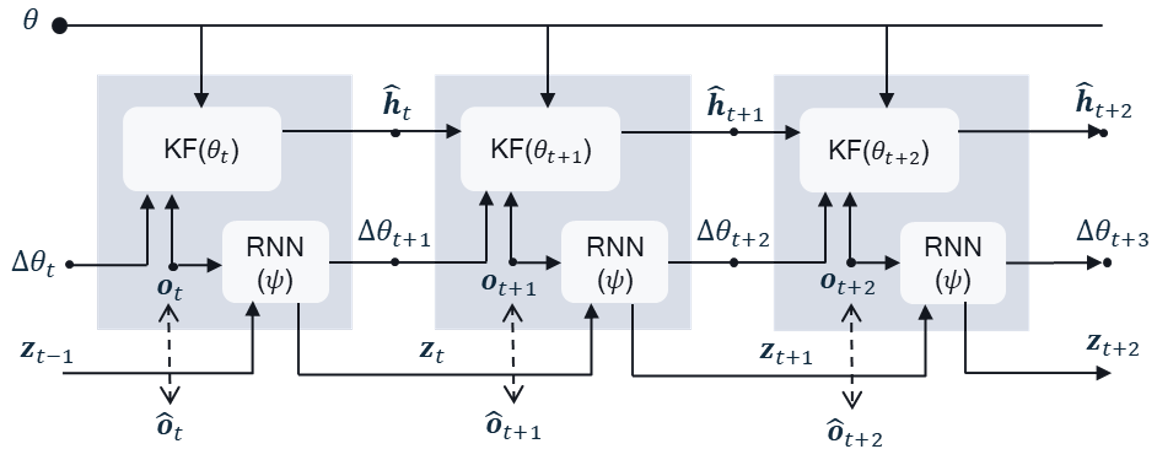
Figure 1: Illustration of Hypernetwork Kalman Filter. Each shaded block represents one inference iteration of the HKF, where $\theta$ denotes the base set of KF parameters around which the RNN models the residual $\Delta\theta_{t}$, $\theta_{t}$ is the final KF parameters at step $t$, ${\bm{z}}_{t}$ is the RNN state variable, ${\bm{o}}_{t}$ and $\hat{{\bm{o}}}_{t}$ are the real and synthetic observation respectively, and $\psi$ represents the trainable parameters of the HKF. The RNN extracts the time varying dynamics of the underlying process and informs the KF, at every step, with the optimal set of KF parameters.

IV Experiments

For channel tracking, we have generated a dataset consisting of $15$ Doppler values and then binned them into $5$ mutually exclusive and collectively exhaustive bins. For binning, we use the genie Doppler information to use the correct bin for each channel sequence. We use MATLAB for dataset generation with CDL-B channel profile. We have used $4096$ tones for OFDM transmission at $4$ GHz carrier frequency, delay spread of $100$ ns, and sub-carrier spacing of $30$ KHz. Table I depicts the binning strategy used for our experiments, i.e., the Doppler values per bin followed by the corresponding User Equipment (UE) relative velocity. Our dataset contains $800$ training channel instances, and $200$ test channel instances per Doppler frequency. Each channel instance is $1500$ OFDM symbols long. Unless specified otherwise, we use an SNR of $10$ dB and a pilot ratio of $1:6$, i.e., a noisy observation at every $6^{th}$ time step. The evaluation metric in our experiments is MNSE as in equation 2 measured in dB unit. Although any RNN can be used, we have used LSTM for the rest. To ensure a fair comparison across different learning based methods, we keep the size of the network hidden state ($z$) at $2N$ for both the RNN and the hypernetwork RNN.

In terms of computational complexity, the HKF has the highest complexity followed by the RNN, further followed by the variants of KF. It should be noted that non-learning based methods, i.e., HKF, and BKF, have an extra computational overhead due to the Doppler estimation unit for Doppler shift estimation but the NN based methods doesn’t need explicit Doppler information as they learn to extract the channel dynamics implicitly from the pilots.

IV-A Evaluation of different channel tracking schemes

In the first experiment, we train one HKF on the entire dataset consisting of all the $15$ Doppler values. To compare HKF against a standalone NN based baseline, we also train an LSTM on the similar settings. We compare both of these learned methods with genie (GKF) and BKF. The parameters of GKF is matched exactly to the Doppler value and obtained using the data generated from the same Doppler. Note that this approach would be prohibitively complex in practice, as we require to keep in infinite bank of Kalman filters, one for each Doppler. On the other hand, as mentioned before, the BKF is an intermediate solution, which only keeps a finite bank of Kalman filters, each one corresponding to a Doppler range. We have chosen five bins presented in Table I. Table II charts the evaluation results on the test data for all the $15$ Doppler values. Our HKF performs consistently better than the standalone LSTM. A single HKF, without any genie Doppler information, outperforms the BKF baseline which requires genie Doppler information and $5$ separate KFs. At higher Doppler frequencies, the HKF even outperforms the GKF, which uses a separate KF per Doppler.

Bin setup
Bin index	Doppler values (Hz)	corresponding velocity (kmph)
Bin 0	0, 30, 60	0.0, 8.0, 16.0
Bin 1	70, 100, 130	18.0, 27.0, 35.0
Bin 2	150, 210, 270	40.5, 56.6, 72.8
Bin 3	300, 400, 500	81.0, 108.0, 135.0
Bin 4	800, 1300, 1850	215.8, 350.7, 499.0

TABLE I: Bin based discretization of Doppler spectrum

MNSE (in dB)
Doppler	GKF	BKF	LSTM	HKF	HKF-2
0 Hz	-48.89	-31.78	-18.05	-29.99	-31.86
30 Hz	-32.60	-32.60	-22.16	-30.59	-30.62
60 Hz	-31.40	-28.47	-26.77	-30.76	-30.92
70 Hz	-30.64	-28.84	-26.63	-30.75	-30.95
100 Hz	-27.71	-30.06	-29.15	-30.80	-31.04
130 Hz	-28.89	-26.96	-29.23	-30.82	-31.22
150 Hz	-29.64	-29.91	-29.30	-30.65	-31.04
210 Hz	-31.76	-30.76	-29.19	-30.62	-30.80
270 Hz	-30.66	-28.61	-29.12	-30.33	-30.44
300 Hz	-29.68	-30.18	-29.27	-30.20	-30.22
400 Hz	-30.24	-29.98	-28.15	-29.48	-29.38
500 Hz	-29.55	-28.85	-27.90	-28.72	-28.63
800 Hz	-26.70	-18.75	-25.59	-26.47	-26.55
1300 Hz	-21.65	-17.59	-22.01	-22.85	-23.24
1850 Hz	-16.86	-15.25	-18.29	-19.18	-19.67

TABLE II: Performance of HKF & HKF-2 (see IV-B) on a range of Doppler values compared against classical and standalone NN based baselines.

IV-B Impact of increasing model capacity

In this experiment, we study the effects of increasing the depth (complexity) of the HKF. We define HKF-2 as HKF but with $2$ layers of LSTM. In Table. II, we observe that increasing the depth of HKF leads to consistent performance boost for $13$ out of $15$ Doppler frequencies. The result suggests that further improvements in the performance can be achieved by increasing the depth of the network.

IV-C Doppler interpolation

In the following experiment, we evaluate the ability of different tracking schemes to interpolate to unseen Doppler scenarios, i.e., Doppler frequencies that are not present in the training dataset. For this experiment, we generate data for one extra Doppler per bin. In case of BKF, we use the genie Doppler information to pick the right bin for each test instance, i.e., we choose the KF belonging to the exact bin to which the test channel belongs. Depicted in Table. III, our HKF and HKF-2 outperform LSTM on all the $5$ Doppler frequencies and outperform BKF at $4$ out of $5$ cases without genie information.

MNSE (in dB)
Doppler	BKF	LSTM	HKF-1	HKF-2
50 Hz	-30.06	-25.58	-30.89	-31.12
120 Hz	-28.12	-27.99	-30.62	-31.05
240 Hz	-29.87	-28.90	-30.49	-30.64
450 Hz	-29.65	-27.63	-29.18	-29.07
1500 Hz	-17.99	-19.52	-20.94	-21.27

TABLE III: Evaluation on untrained Doppler values

This result is in agreement with our postulate that the HKF brings together the flexibility of the RNNs with out of domain generalization capability of the KF. The proposed HKF demonstrates better Doppler interpolation properties than both the classical baseline and solely NN based baseline. In the current experiment, the HKF-2 consistently outperforms the HKF-1, hence, we use HKF-2 for the next experiments.

IV-D Generalization properties

In the next experiments, we investigate the performance of different schemes when extrapolated to settings beyond the training scenario. For the sake of completeness, we introduce HKF-G, a global version of HKF-2. The HKF-G shares the same model with HKF-2, but unlike HKF-2 which is trained on a single SNR value of $10$ dB and a pilot ratio of $1:6$, HKF-G is trained on SNR values uniformly sampled from the range $5-15$ dB and pilot ratios uniformly sampled from the set $\{1:3,1:5,1:6,1:8,1:10\}$. The idea is to see how much gain we get by training on a range of different scenarios.

IV-D1 Generalization to untrained pilot ratios

We start with generalization to different untrained pilot ratios. Table. IV shows the evaluation results when both the LSTM and HKF-2, trained on a pilot ratio of $1:6$, are evaluated on a pilot ratio of $1:3$. An increased pilot frequency means more frequent observations of the underlying channel. Intuitively, increase in pilot frequency should lead to better channel estimates. As depicted in upper half of Table. IV, the performance of HKF-2 improves by increasing the pilot frequency and it still remains competitive to the BKF. On the other hand, despite the more frequent observations, the LSTM completely collapses.

To increase the scope of our findings, we also evaluated our methods on unseen Doppler values combined with an untrained pilot ratio. The lower half of Table. IV depicts the results when different schemes are evaluated on untrained Doppler values combined with an untrained pilot ratio of $1:3$. For both the seen and unseen Doppler scenarios, the HKF-2 performs competitive to the BKF while the LSTM fails to generalize. The HKF-G, which includes this pilot ratio in the training phase, performs the best among others.

MNSE (in dB)
Seen Doppler values
Doppler	BKF	LSTM	HKF-2	HKF-G
0 Hz	-35.33	-18.63	-34.77	-35.15
30 Hz	-34.80	-20.64	-33.42	-33.91
60 Hz	-31.33	-20.21	-33.11	-33.47
70 Hz	-31.96	-20.16	-33.11	-33.39
100 Hz	-33.04	-18.67	-33.60	-33.93
130 Hz	-30.48	-17.27	-33.53	-33.74
150 Hz	-33.09	-16.16	-33.41	-33.62
210 Hz	-33.40	-14.50	-33.39	-33.63
270 Hz	-32.19	-13.18	-32.94	-33.15
300 Hz	-33.19	-12.65	-32.72	-32.95
400 Hz	-32.90	-11.33	-32.08	-32.36
500 Hz	-32.26	-10.57	-31.51	-31.90
800 Hz	-28.06	-10.52	-29.61	-30.43
1300 Hz	-27.18	-9.83	-27.07	-28.45
1850 Hz	-25.30	-7.60	-24.17	-26.53
Unseen Doppler values
50 Hz	-32.60	-20.66	-33.27	-33.68
120 Hz	-31.51	-17.68	-33.63	-33.89
240 Hz	-32.87	-13.70	-33.18	-33.40
450 Hz	-32.69	-10.90	-31.85	-32.15
1500 Hz	-27.28	-7.71	-25.40	-27.04

TABLE IV: Evaluation on untrained pilot ratio of $1:3$

In the preceding experiment, we experimented with an increased pilot frequency of $1:3$. In the following experiment, we perform a similar experiment but with a reduced pilot frequency of $1:10$. Intuitively, a decrease in pilot frequency would lead to degradation in the performance as there are less frequent observations available to estimate the channel. Table.V depicts the results when different schemes are evaluated on an untrained pilot ratio of $1:10$ combined with seen and unseen Doppler instances. Similar to the previous results, the HKF-2 remains competitive to the BKF while the LSTM collapses. Owing to its more diverse training, the HKF-G fares much better than the other tracking methods.

MNSE (in dB)
Seen Doppler values
Doppler	BKF	LSTM	HKF-2	HKF-G
0 Hz	-28.56	-4.55	-20.44	-26.16
30 Hz	-31.70	-5.55	-19.52	-26.93
60 Hz	-25.80	-4.85	-18.62	-27.29
70 Hz	-26.16	-4.31	-20.68	-25.30
100 Hz	-27.59	-3.29	-23.47	-27.39
130 Hz	-23.34	-2.11	-23.56	-27.17
150 Hz	-26.00	-1.34	-25.07	-27.63
210 Hz	-27.90	-0.32	-24.87	-27.60
270 Hz	-24.41	0.34	-25.54	-27.22
300 Hz	-26.77	0.54	-21.16	-27.09
400 Hz	-26.86	1.07	-24.04	-25.95
500 Hz	-24.77	1.34	-23.30	-24.71
800 Hz	-10.36	1.95	-18.95	-20.80
1300 Hz	-9.50	2.19	-10.90	-15.45
1850 Hz	-7.25	2.23	-5.18	-11.10
Unseen Doppler values
50 Hz	-27.74	-5.11	-23.34	-24.83
120 Hz	-25.32	-2.39	-23.31	-27.41
240 Hz	-26.43	0.07	-24.40	-27.38
450 Hz	-26.28	1.19	-24.14	-25.38
1500 Hz	-10.21	2.22	-8.08	-12.28

TABLE V: Evaluation on untrained pilot ratio of $1:10$

IV-D2 Generalization to untrained SNR values

In the following experiments, we study the generalization properties of different schemes to different noise levels. Both the LSTM, and the HKFs, trained on an SNR of $10$ dB, are evaluated on two different SNRs of $5$ dB and $15$ dB. Table. VI shows the finding when different schemes are evaluated on an untrained SNR of $5$ dB with seen and unseen Doppler instances. Evident from the Table. VI, the performance of LSTM degrades significantly. On the other hand, the HKF-2 performs comparable to the HKF-G and even outperforms the BKF at certain instances.

MNSE (in dB)
Seen Doppler values
Doppler	BKF	LSTM	HKF-2	HKF-G
0 Hz	-28.62	-15.83	-27.15	-28.84
30 Hz	-29.81	-17.18	-27.30	-28.44
60 Hz	-25.08	-18.46	-27.79	-28.65
70 Hz	-25.67	-18.11	-27.85	-28.56
100 Hz	-26.56	-18.81	-27.92	-28.57
130 Hz	-23.50	-18.64	-27.99	-28.47
150 Hz	-26.88	-18.83	-27.81	-28.31
210 Hz	-27.32	-19.26	-27.54	-28.13
270 Hz	-25.59	-19.81	-27.07	-27.69
300 Hz	-26.83	-19.68	-26.79	-27.50
400 Hz	-26.57	-19.44	-25.92	-26.78
500 Hz	-25.63	-19.52	-25.13	-26.16
800 Hz	-17.90	-19.42	-23.64	-24.19
1300 Hz	-16.77	-16.94	-20.93	-21.31
1850 Hz	-14.62	-14.83	-18.20	-18.31
Unseen Doppler values
50 Hz	-26.61	-18.17	-27.74	-28.64
120 Hz	-24.64	-18.59	-27.91	-28.49
240 Hz	-26.58	-19.18	-27.29	-27.79
450 Hz	-26.28	-19.58	-25.55	-26.40
1500 Hz	-17.17	-14.85	-19.23	-19.37

TABLE VI: Evaluation on untrained SNR of $5$ dB

Next, we evaluate different methods on an untrained SNR of $15$ dB. Tables. VII charts the findings of our experiments when different schemes are evaluated on seen and unseen Doppler scenarios. Similar to the prior experiment, the LSTM fails to generalize to a new SNR while the HKF-G performs the best. The HKF-2, despite being trained on a single SNR ($10$ dB) far away from the test SNRs ($5$ dB and $10$ dB), performs competitive to the HKF-G and BKF. The HKF-2 performs comparable to BKF in low-to-mid frequency range and outperforms it at higher frequency range.

MNSE (in dB)
Seen Doppler values
Doppler	BKF	LSTM	HKF-2	HKF-G
0 Hz	-34.00	-18.76	-33.70	-33.26
30 Hz	-34.56	-22.61	-31.84	-32.01
60 Hz	-31.08	-27.59	-32.11	-32.34
70 Hz	-30.96	-29.33	-32.24	-32.44
100 Hz	-32.84	-31.31	-32.16	-32.63
130 Hz	-29.53	-31.72	-32.59	-32.89
150 Hz	-32.29	-30.41	-32.46	-32.65
210 Hz	-33.98	-30.74	-32.24	-32.62
270 Hz	-31.05	-29.89	-31.82	-32.08
300 Hz	-33.28	-31.56	-31.55	-31.90
400 Hz	-33.22	-29.48	-30.59	-31.01
500 Hz	-31.71	-29.95	-29.69	-30.12
800 Hz	-19.11	-23.72	-27.74	-27.72
1300 Hz	-17.95	-23.10	-24.18	-23.92
1850 Hz	-15.52	-18.98	-20.08	-19.62
Unseen Doppler values
50 Hz	-32.78	-27.08	-32.44	-32.59
120 Hz	-30.79	-29.08	-32.28	-32.74
240 Hz	-32.79	-30.36	-32.05	-32.37
450 Hz	-32.80	-29.14	-30.20	-30.62
1500 Hz	-18.35	-20.15	-21.82	-21.29

TABLE VII: Evaluation on untrained SNR of $15$ dB

V Conclusion

Exclusive neural network based solutions to channel tracking problem generalize poorly to unseen scenarios with significant performance degradation. On the other hand, although Kalman filter generalizes well to different SNR and observation patterns, it needs to be adapted continually to changing channel dynamics. We propose a hypernetwork Kalman filter solution which reconciles the best part of both approaches. It was shown that a single HKF could be used on a wide range of Doppler values with good out of domain generalization. We believe these neural augmentation approaches are well suited for maximal utilization of the domain knowledge.

References

- [1] A. Barbieri, A. Piemontese, and G. Colavolpe, “On the ARMA approximation for fading channels described by the Clarke model with applications to Kalman-based receivers,” IEEE Transactions on Wireless Communications, vol. 8, no. 2, pp. 535–540, Feb. 2009.
- [2] S. Kashyap, C. Mollén, E. Björnson, and E. G. Larsson, “Performance analysis of (TDD) massive MIMO with Kalman channel prediction,” in 2017 IEEE International Conference on Acoustics, Speech and Signal Processing (ICASSP), Mar. 2017, pp. 3554–3558.
- [3] A. H. El Husseini, E. P. Simon, and L. Ros, “Optimization of the second order autoregressive model AR(2) for Rayleigh-Jakes flat fading channel estimation with Kalman filter,” in 2017 22nd International Conference on Digital Signal Processing (DSP), Aug. 2017, pp. 1–5.
- [4] V. G. Satorras, M. Welling, and Z. Akata, “Combining Generative and Discriminative Models for Hybrid Inference,” in Advances in Neural Information Processing Systems 33, 2019, p. 11.
- [5] ETSI 3rd Generation Partnership Project (3GPP), “Study on channel model for frequency spectrum above 6 ghz,” 3GPP TR 38.900, Jun, Tech. Rep., 2016.
- [6] M. Karl, M. Soelch, J. Bayer, and P. v. d. Smagt, “Deep Variational Bayes Filters: Unsupervised Learning of State Space Models from Raw Data,” in ICLR 2017, Nov. 2016.
- [7] R. Krishnan, U. Shalit, and D. Sontag, “Structured inference networks for nonlinear state space models,” in Proceedings of the AAAI Conference on Artificial Intelligence, vol. 31, no. 1, 2017.
- [8] E. de Bézenac, S. S. Rangapuram, K. Benidis, M. Bohlke-Schneider, R. Kurle, L. Stella, H. Hasson, P. Gallinari, and T. Januschowski, “Normalizing Kalman Filters for Multivariate Time Series Analysis,” in Neural Information Processing Systems, 2020, p. 13.
- [9] H. Coskun, F. Achilles, R. DiPietro, N. Navab, and F. Tombari, “Long short-term memory kalman filters: Recurrent neural estimators for pose regularization,” in Proceedings of the IEEE International Conference on Computer Vision, 2017, pp. 5524–5532.
- [10] S. S. Rangapuram, M. W. Seeger, J. Gasthaus, L. Stella, Y. Wang, and T. Januschowski, “Deep State Space Models for Time Series Forecasting,” in Advances in Neural Information Processing Systems, vol. 31, 2018, pp. 7785–7794.
- [11] T. Kailath, Lectures on Wiener and Kalman Filtering. Vienna: Springer Wien, 2014.
- [12] D. P. Kingma and M. Welling, “Auto-encoding variational bayes,” arXiv preprint arXiv:1312.6114, 2013.