Deep Reinforcement Learning for Wireless Scheduling in Distributed Networked Control

Abstract

We consider a joint uplink and downlink scheduling problem of a fully distributed wireless networked control system (WNCS) with a limited number of frequency channels. Using elements of stochastic systems theory, we derive a sufficient stability condition of the WNCS, which is stated in terms of both the control and communication system parameters. Once the condition is satisfied, there exists a stationary and deterministic scheduling policy that can stabilize all plants of the WNCS. By analyzing and representing the per-step cost function of the WNCS in terms of a finite-length countable vector state, we formulate the optimal transmission scheduling problem into a Markov decision process and develop a deep-reinforcement-learning-based algorithm for solving it. Numerical results show that the proposed algorithm significantly outperforms benchmark policies.

I Introduction

The Fourth Industrial Revolution, Industry 4.0, is the automation of conventional manufacturing and industrial processes through flexible mass production. Eliminating the communication wires in traditional factories is a game-changer, as large-scale, interconnected deployment of massive spatially distributed industrial devices are required for automatic control in Industry 4.0, including sensors, actuators, machines, robots, and controllers. With high-scalable and low-cost deployment capabilities, wireless networked control is one of the most important technologies of Industry 4.0, enabling many industrial applications, such as smart city, smart manufacturing, smart grids, e-commerce warehouses and industrial automation systems [1, 2].

Unlike traditional cable-based networked control systems, in a large-scale wireless networked control system (WNCS), communication resources are limited. Not surprisingly, during the past decade, transmission scheduling in WNCS has drawn a lot of attention in the research community. Focusing on the sensor-controller communications only (the controller-actuator co-located scenario), the optimal transmission scheduling problem of over a single frequency channel for achieving the best remote estimation quality was extensively investigated in [3, 4, 5, 6]. For the multi-frequency channel scenario, the optimal scheduling policy and structural results were obtained in [7]. The optimal transmission power scheduling problem of an energy-constrained remote estimation system was studied in [8]. The joint scheduling and power allocation problems of multi-plant-multi-frequency WNCSs were investigated in [9, 10] for achieving the minimum overall transmission power consumption. From a cyber-physical security perspective, denial-of-service (DoS) attackers’ scheduling problems were investigated in [11, 12], for maximally deteriorating the WNCSs’ performance.

In the WNCS examined in the above works, classic dynamic programming (including policy and value iteration and Q-learning) are the most commonly considered approaches for solving scheduling problems in small scale. For example, numerical results of the optimal scheduling of a two-sensor-one-frequency system were presented in [7]. However, due to Bellman’s curse of dimensionality [13], such methods cannot be directly applied to solve dynamic programming problems of large scale WNCSs. Fortunately, the curse of dimensionality can be addressed by the use of function approximations. Deep reinforcement learning (DRL) using deep neural networks as function approximators is a promising technique for solving large decision making problems [14]. Some recent works [15, 16] have applied DRL methods to solve multi-system-multi-frequency scheduling problems in different WNCS scenarios. Apart from scheduling problems, DRL has also been applied for joint control and communications design in WNCSs [17, 18].

We note that most of the existing works only focus on WNCSs which are only partially distributed [3, 4, 5, 7, 9, 10, 15, 16]. In a fully distributed setting, both downlink (controller-actuator) and uplink (sensor-controller) transmissions are crucial for stabilizing each plant. It is surprising that, while spatial diversity is a common phenomenon in practical wireless environments [19], existing transmission scheduling works for achieving the optimal control system performance commonly ignore the spatial diversity of different communication links by assuming identical channel condition (e.g., packet error probabilities) for different links at the same frequency.

In this paper, we investigate the transmission scheduling problem of distributed WNCS. The main contributions are summarized as follows:

• We propose a distributed $N$-plant-$M$-frequency WNCS model, where the controller schedules the uplink and downlink transmissions of all $N$ plants and the spatial diversity of different communication links are taken into account. The controller generates sequential predictive control commands for each of the plants based on pre-designed deadbead control laws. Different from uplink or downlink only scheduling, a joint scheduling algorithm has a larger action space and also needs to automatically balance the tradeoff between the uplink and the downlink due to the communication resource limit. To the best of our knowledge, joint uplink and downlink transmission scheduling of distributed WNCSs has not been investigated in the open literature.

• We derive a sufficient stability condition of the WNCS in terms of both the control and communication system parameters. The result provides a theoretical guarantee that there exists at least one stationary and deterministic scheduling policy that can stabilize all plants of the WNCS. We show that the obtained condition is also necessary in the absence of spatial diversity of different communication links.

• We construct a finite-length countable vector state of the WNCS in terms of the time duration between consecutive received packets at the controller and the actuators. Then, we prove that the per-step cost function of the WNCS is determined by the time-duration-related vector state. Building on this, we formulate the optimal transmission scheduling problem into a Markov decision process (MDP) problem with an countable state space for achieving the minimum expected total discounted cost. We propose an effective action space reduction method and use a DRL-based algorithm for solving the problem. Numerical results illustrate that the proposed algorithm can reduce the expected cost significantly compared to available benchmark policies.

Notations: $\sum_{m=i}^{j}a_{m}\triangleq 0$ if $i>j$. $\limsup_{K\rightarrow\infty}$ is the limit superior operator. $\mathsf{C}^{k}_{n}\triangleq\frac{n!}{k!(n-k)!}$ and $\mathsf{P}^{k}_{n}\triangleq\frac{n!}{(n-k)!}$ are the numbers of combinations and permutations of $n$ things taken $k$ at a time, respectively. $\text{Tr}(\mathbf{A})$ and $\mathsf{rank}[\mathbf{A}]$ denote the trace and the rank of matrix $\mathbf{A}$, respectively.

II Distributed WNCS with Shared Wireless Resource

We consider a distributed WNCS system with $N$ plants and a central controller as illustrated in Fig. 1. The output of plant $i$ is measured by smart sensor $i$, which sends pre-filtered measurements (local state estimates) to the controller. The controller applies a remote (state) estimator and a control algorithm for plant $i$. It then generates and sends a control signal to actuator $i$, thereby closing the loop. A key limitation of the WNCS is that smart sensor $i$ cannot communicate with actuator $i$ directly due to the spatial deployment. Instead, the uplink (sensor-controller) and downlink (controller-actuator) communications for the $N$ plants share a common wireless network with only $M$ frequency channels, where $M<2N$. Thus, not every node is allowed to transmit at the same time and communications need to be scheduled. As shown in Fig. 1, we shall focus on a setup where scheduling is done at the controller side, which schedules both the downlink and uplink transmissions.

Each smart sensor has three modules: remote estimator, control algorithm and local Kalman filter. The first two modules are copies of the ones at the controller to reconstruct the control input of the plant. Such information is sent to the Kalman filter for accurate local state estimation. The details will be presented in the sequel.

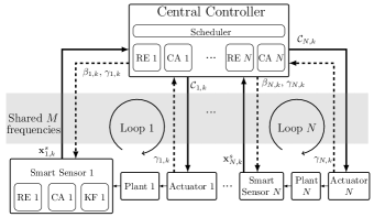
Figure 1: A distributed networked control system with $N$ plants sharing $M$ frequency channels. Kalman filter, remote estimator and control algorithm are denoted as KF, RE and CA and discussed in Sections II-B, II-C and II-D, respectively.

II-A Plant Dynamics

The $N$ plants are modeled as linear time-invariant (LTI) discrete-time systems as [9, 16]

$$\mathbf{x}_{i,k+1}=\mathbf{A}_{i}\mathbf{x}_{i,k}+\mathbf{B}_{i}\mathbf{u}_{i,k}+\mathbf{w}_{i,k},$$ (1)

$$\mathbf{y}_{i,k}=\mathbf{C}_{i}\mathbf{x}_{i,k}+\mathbf{v}_{i,k},\quad i=1,\cdots,N$$

where $\mathbf{x}_{i,k}\in\mathbb{R}^{n_{i}}$ and $\mathbf{u}_{i,k}\in\mathbb{R}^{m_{i}}$ are the state vector of plant $i$ and the control input applied by actuator $i$ at time $k$, respectively. $\mathbf{w}_{i,k}\in\mathbb{R}^{n_{i}}$ is the $i$-th plant disturbance and is an independent and identically distributed (i.i.d.) zero-mean Gaussian white noise process with covariance matrix $\mathbf{Q}_{i}^{w}\in\mathbb{R}^{n_{i}\times n_{i}}$. $\mathbf{A}_{i}\in\mathbb{R}^{n_{i}\times n_{i}}$ and $\mathbf{B}_{i}\in\mathbb{R}^{n_{i}\times m_{i}}$ are the system-transition matrix and control-input matrix for plant $i$, respectively. $\mathbf{y}_{i,k}\in\mathbb{R}^{p_{i}}$ is sensor $i$’s measurement of plant $i$ at time $k$ and $\mathbf{v}_{i,k}\in\mathbb{R}^{p_{i}}$ is the measurement noise, modeled as an i.i.d. zero-mean Gaussian white noise process with covariance matrix $\mathbf{Q}_{i}^{v}\in\mathbb{R}^{p_{i}\times p_{i}}$. $\mathbf{C}_{i}\in\mathbb{R}^{p_{i}\times n_{i}}$ is the measurement matrix of plant $i$. We assume that plant $i$ is $v_{i}$-step controllable, $\forall i\in\{1,\dots,N\}$ [21], i.e., there exists a control gain $\tilde{\mathbf{K}}_{i}$ satisfying

$$(\mathbf{A}_{i}+\mathbf{B}_{i}\tilde{\mathbf{K}}_{i})^{v_{i}}=\mathbf{0}.$$ (2)

Note that when $\mathbf{A}_{i}$ is non-singular, the system (1) is $v_{i}$-step controllable if and only if

$$\mathsf{rank}\left[\mathbf{A}^{-1}_{i}\mathbf{B}_{i},\mathbf{A}^{-2}_{i}\mathbf{B}_{i},\dots,\mathbf{A}^{-v_{i}}_{i}\mathbf{B}_{i}\right]=n_{i}.$$ (3)

The details of the control algorithm will be given in Section II-D.

II-B Smart Sensors

Due to the noise measurement, each smart sensor runs a Kalman filter to estimate the current plant state as below [22]:

$$\mathbf{x}^{s}_{k|k-1} =\mathbf{A}\mathbf{x}^{s}_{k-1}+\mathbf{B}\mathbf{u}_{k-1}$$ (4)

$$\mathbf{P}^{s}_{k|k-1} =\mathbf{A}\mathbf{P}^{s}_{k-1}\mathbf{A}^{\top}+\mathbf{Q}^{w}$$

$$\mathbf{K}_{k} =\mathbf{P}^{s}_{k|k-1}\mathbf{C}^{\top}(\mathbf{C}\mathbf{P}^{s}_{k|k-1}\mathbf{C}^{\top}+\mathbf{Q}^{v})^{-1}$$

$$\mathbf{x}^{s}_{k} =\mathbf{x}^{s}_{k|k-1}+\mathbf{K}_{k}(\mathbf{y}_{k}-\mathbf{C}\mathbf{x}^{s}_{k|k-1})$$

$$\mathbf{P}^{s}_{k} =(\mathbf{I}-\mathbf{K}_{k}\mathbf{C})\mathbf{P}^{s}_{k|k-1}$$

where $\mathbf{x}^{s}_{k|k-1}$ and $\mathbf{x}^{s}_{k}$ are the prior and posterior state estimation at time $k$, respectively, and $\mathbf{P}^{s}_{k|k-1}$ and $\mathbf{P}^{s}_{k}$ are the (estimation error) covariances of $\mathbf{e}^{s}_{k|k-1}\triangleq\mathbf{x}_{k}-\mathbf{x}^{s}_{k|k-1}$ and $\mathbf{e}^{s}_{k}\triangleq\mathbf{x}_{k}-\mathbf{x}^{s}_{k}$, respectively. $\mathbf{K}_{k}$ is the Kalman gain at time $k$. We assume that each $(\mathbf{A},\mathbf{C})$ is observable and $(\mathbf{A},\mathbf{Q}^{w})$ is controllable [7]. Thus, the Kalman gain $\mathbf{K}_{k}$ and error covariance matrix $\mathbf{P}^{s}_{k}$ converge to constant matrices $\hat{\mathbf{K}}$ and $\hat{\mathbf{P}}^{s}$, respectively, i.e., the smart sensor is in the stationary mode. As foreshadowed, the smart sensor employs a remote estimator and knowledge of the control algorithm that is applied at the controller side to obtain the control input in (4). Thus, the Kalman filter (4) is the optimal estimator of the linear system (1) in terms of the estimation mean-square error [23]. The remote estimator and control algorithm will be presented in Sections II-C and II-D, respectively.

As shown in Fig. 1, at every scheduling instant $k$, the smart sensor sends the local estimate ${\mathbf{x}}_{k}^{s}$ (rather than the raw measurement $\mathbf{y}_{k}$) to the controller.

Before proceeding, we note that (4) leads to the following recursion for the estimation error at the sensors:

$$\mathbf{e}^{s}_{k+1|k}=\mathbf{A}\mathbf{e}^{s}_{k}+\mathbf{w}_{k}$$ (5)

$$\mathbf{e}^{s}_{k}=\big{(}\mathbf{I}-\hat{\mathbf{K}}\mathbf{C}\big{)}\mathbf{e}^{s}_{k|k-1}-\hat{\mathbf{K}}\mathbf{v}_{k}$$ (6)

and hence

$$\mathbf{e}^{s}_{k}=\big{(}\mathbf{I}-\hat{\mathbf{K}}\mathbf{C}\big{)}\mathbf{A}\mathbf{e}^{s}_{k-1}+\big{(}\mathbf{I}-\hat{\mathbf{K}}\mathbf{C}\big{)}\mathbf{w}_{k-1}-\hat{\mathbf{K}}\mathbf{v}_{k}.$$ (7)

Then, the relation between the estimation errors $\mathbf{e}_{k}^{s}$ and $\mathbf{e}_{k-K}^{s}$, $\forall K\in\mathbb{N}$, is established as

$$\mathbf{e}^{s}_{k} \!=\!\mathbf{Z}^{K}\mathbf{e}^{s}_{k-\!K}\!+\!\!\sum_{i=1}^{K}\mathbf{Z}^{i\!-\!1}\big{(}\mathbf{I}\!-\!\hat{\mathbf{K}}\mathbf{C}\big{)}\mathbf{w}_{k-\!i}\!-\!\!\sum_{i=1}^{K}\mathbf{Z}^{i-\!1}\hat{\mathbf{K}}\mathbf{v}_{k\!-i+1},$$ (8)

where $\mathbf{Z}\triangleq\big{(}\mathbf{I}-\hat{\mathbf{K}}\mathbf{C}\big{)}\mathbf{A}$.

II-C Remote Estimation

The controller applies a minimum mean-square error (MMSE) remote estimator for each plant taking into account the random packet dropouts and one-step transmission delay as [22]:

$$\hat{\mathbf{x}}_{i,k+1}=\begin{cases}\mathbf{A}_{i}\mathbf{x}^{s}_{i,k}+\mathbf{B}_{i}\mathbf{u}_{i,k}&\mbox{ if }\beta_{i,k}=1\\ \mathbf{A}_{i}\hat{\mathbf{x}}_{k}+\mathbf{B}_{i}\mathbf{u}_{i,k}&\mbox{ if }\beta_{i,k}=0\\ \end{cases}$$ (9)

where $\beta_{i,k}=1$ or $0$ indicates that the controller receives sensor $i$’s packet or not at time $k$, respectively. Then, the estimation error $\mathbf{e}_{i,k}$ is obtained as

$$\mathbf{e}_{i,k}\triangleq\mathbf{x}_{i,k}-\hat{\mathbf{x}}_{i,k}=\begin{cases}\mathbf{A}_{i}\mathbf{e}^{s}_{i,k-1}+\mathbf{w}_{i,k-1}&\mbox{ if }\beta_{i,k-1}=1\\ \mathbf{A}_{i}\mathbf{e}_{i,k-1}+\mathbf{w}_{i,k-1}&\mbox{ if }\beta_{i,k-1}=0\end{cases}$$ (10)

From (9), the controller’s current estimation depends on the most recently received sensor estimation. Let $\tau_{i,k}\in\{1,2,\cdots\}$ denote the age-of-information (AoI) (see [24] and reference therein) of sensor $i$’s packet observed at time $k$, i.e., the number of elapsed time slots from the latest successfully delivered sensor $i$’s packet before the current time $k$, which reflects how old the most recently received sensor measurement is. Then, it is easy to see that the updating rule of $\tau_{i,k}$ is given by

$$\tau_{i,k+1}=\begin{cases}1&\mbox{ if }\beta_{i,k}=1\\ \tau_{i,k}+1&\mbox{ otherwise.}\end{cases}$$ (11)

Using (10) and the AoI, the relation between the local and remote estimation error can be characterized by:

$$\mathbf{e}_{i,k}=\mathbf{A}_{i}^{\tau_{i,k}}\mathbf{e}^{s}_{i,k-\tau_{i,k}}+\sum_{j=1}^{\tau_{i,k}}\mathbf{A}_{i}^{j-1}\mathbf{w}_{k-j}.$$ (12)

II-D Control Algorithm

Due to the fact that downlink transmissions are unreliable, actuator $i$ may not receive the controller’s control-command-carrying packets, even when transmissions are scheduled. We adopt a predictive control approach [21, 25] to provide robustness against packet failures: the controller sends a length-$v_{i}$ sequence of control commands including both the current command and the predicted future commands to the actuator once scheduled; if the current packet is lost, the actuator will apply the previously received predictive command for the current time slot as the control input.

The control sequence for plant $i$ is generated by a linear deadbeat control gain $\tilde{\mathbf{K}}_{i}$ as [21]

$$\mathcal{C}_{i,k}=\big{[}\tilde{\mathbf{K}}_{i}\hat{\mathbf{x}}_{i,k},\tilde{\mathbf{K}}_{i}\mathbf{\Phi}_{i}\hat{\mathbf{x}}_{i,k},\cdots,\tilde{\mathbf{K}}_{i}(\mathbf{\Phi}_{i})^{v_{i}-1}\hat{\mathbf{x}}_{i,k}\big{]}$$ (13)

where $\mathbf{\Phi}_{i}\triangleq\mathbf{A}_{i}+\mathbf{B}_{i}\tilde{\mathbf{K}}_{i}$ and $\tilde{\mathbf{K}}_{i}$ satisfies $(\mathbf{A}_{i}+\mathbf{B}_{i}\tilde{\mathbf{K}}_{i})^{v_{i}}=\mathbf{0},$ and $v_{i}$ is the controllability index of the pair $(\mathbf{A}_{i},\mathbf{B}_{i})$. Note that the first element in $\mathcal{C}_{i,k}$ is the current control command and the rest are the predicted ones.

Remark 1.

It can be verified that if the current state estimation $\hat{\mathbf{x}}_{i,k}$ is perfect and the plant $i$ is disturbance free, then the plant state $\mathbf{x}_{i,k}$ would be set to zero after applying all $v_{i}$ steps of the control sequence in (13). Such a deadbeat controller is commonly considered as a time-optimal controller that takes the minimum time for setting the current plant state to the origin [26]. We note that the deadbeat control law may not be cost-optimal, and the optimal control law may depend on the scheduling policy. Since the current work focuses on transmission scheduling design of the $N$-plant-$M$-frequency WNCS, the optimal joint control-scheduling problem can be investigated in our future work.

Accordingly, actuator $i$ maintains a length-$v_{i}$ buffer

$$\mathcal{U}_{i,k}\triangleq[\mathbf{u}_{i,k}^{0},\mathbf{u}_{i,k}^{1},\cdots,\mathbf{u}_{i,k}^{v_{i}-1}]$$ (14)

to store the received control commands. If the current control packet is received, the buffer is reset with received sequence; otherwise, it is shifted one step forward as

$$\mathcal{U}_{i,k}=\begin{cases}\mathcal{C}_{i,k},&\mbox{ if }\gamma_{i,k}=1\\ [\mathbf{u}_{i,k-1}^{1},\mathbf{u}_{i,k-1}^{2},\cdots,\mathbf{u}_{i,k-1}^{v_{i}},\mathbf{0}],&\mbox{ if }\gamma_{i,k}=0\\ \end{cases}$$ (15)

where $\gamma_{i,k}=1$ or $0$ indicate that actuator $i$ receives a control packet or not at time $k$, respectively. The first command in the buffer is applied as the control input each time

$$\mathbf{u}_{i,k}\triangleq\mathbf{u}_{i,k}^{0}.$$ (16)

Let $\eta_{i,k}\in\{1,2,\cdots\}$ denote the AoI of controller’s packet at actuator $i$ observed at time $k$, i.e., the number of passed time slots (including the current time slot) since the latest received control packet by actuator $i$. Its updating rule is given as

$$\eta_{i,k}=\begin{cases}1,&\mbox{ if }\gamma_{i,k}=1\\ \eta_{i,k-1}+1&\mbox{ if }\gamma_{i,k}=0\end{cases}$$ (17)

From (13) and (15), and by using the deadbeat control property (2), the applied control input can be concisely written as

$$\mathbf{u}_{i,k}=\tilde{\mathbf{K}}_{i}(\mathbf{\Phi}_{i})^{\eta_{i,k}-1}\hat{\mathbf{x}}_{i,k+1-\eta_{i,k}}.$$ (18)

II-E Communication Scheduler

The $N$-plant WNCS has $N$ uplinks and $N$ downlinks sharing $M$ frequencies. Each frequency can be occupied by at most one link, and each link can be allocated to at most one frequency at a time. Let $a_{m,k}\in\{-N,\dots,0,\dots,N\}$ denote the allocated link to frequency $m$ at time $k$, where $a_{m,k}=i^{\prime}$ means the frequency is allocated to $|i^{\prime}|$-th plant, where $i^{\prime}>0$ and $<0$ indicate for uplink and downlink, respectively, and $i^{\prime}=0$ denotes that the frequency channel is idle.

The packet transmissions of each link are modeled as i.i.d. packet dropout processes. Unlike most of the existing works wherein transmission scheduling of WNCSs assumes that different node transmissions at the same frequency channel have the same packet drop probability [15], we here consider a more practical scenario by taking into account the spatial diversity of different transmission nodes – each frequency has different dropout probabilities for different uplink and downlink transmissions. The packet success probabilities of the uplink and downlink of plant $i$ at frequency $m$ are given by $\xi^{s}_{m,i}$ and $\xi^{c}_{m,i}$, respectively, where

$$\xi^{s}_{m,i}\triangleq\mathbb{P}[\beta_{i,k}=1|a_{m,k}=i],$$ (19)

$$\xi^{c}_{m,i}\triangleq\mathbb{P}[\gamma_{i,k}=1|a_{m,k}=-i].$$

The packet success probabilities can be estimated by the controller based on standard channel estimation techniques [19, 27], and are utilized by the MDP and DRL-based solutions in Section IV-C and Section V.

Acknowledgment feedback. We also assume that the actuator sends one-bit feedback signal of $\gamma_{i,k}$ to the controller, and the controller sends $\beta_{i,k}$ as well as $\gamma_{i,k}$ to sensor $i$ each time with negligible overhead. From $\{\beta_{i,k}\}$ and (9), the smart sensor knows the estimated plant state by the controller; using $\{\gamma_{i,k}\}$ and (18), the sensor can calculate the applied control input $\mathbf{u}_{i,k}$, which is utilized for local state estimation as mentioned in Section II-B.

III Stability Condition

Before turning to designing scheduling policies, it is critical to elucidate conditions that the WNCS needs to satisfy which ensure that there exists at least one stationary and deterministic scheduling policy that can stabilize all plants using the available network resources. Note that a policy $\pi$ is a function mapping from a state to an action. A deterministic policy means that the function gives the same action when the input state is fixed. A stationary policy means the function $\pi$ is time invariant, i.e., $\pi_{k}=\pi,\forall k$. In other words, the action only depends on the state, not the time [13]. We adopt a very commonly considered stochastic stability condition as below.

Assumption 1.

The expected initial quadratic norm of each plant state is bounded, i.e., $\mathbb{E}[\mathbf{x}_{i,0}^{\top}\mathbf{x}_{i,0}]<\infty,\forall i=1,\dots,N$.

Definition 1 (Mean-Square Stability).

The WNCS is mean-square stable under Assumption 1 if and only if

$$\limsup_{K\rightarrow\infty}\frac{1}{K}\sum_{k=1}^{K}\mathbb{E}[\mathbf{x}_{i,k}^{\top}\mathbf{x}_{i,k}]<\infty,\forall i=1,\dots,N.$$ (20)

Intuitively, the stability condition of the WNCS should depend on both the (open-loop) unstable plant systems (i.e., those where $\rho(\mathbf{A}_{i})\geq 1$) and the $M$-frequency communication system parameters. For the tractability of sufficient stability condition analysis (i.e., to prove the existence of a stabilizing policy), we focus on policy class that groups the unstable plants into $M$ disjoint sets $\mathcal{F}_{1},\dots,\mathcal{F}_{M}$ and allocates them to the $M$ frequencies, accordingly. Let $\bar{\mathcal{F}}\triangleq\{i:\rho(\mathbf{A}_{i})\geq 1,i\in\{1,\dots,N\}\}$ denote the index set of all unstable plants. We have $\mathcal{F}_{1}\cup\dots\cup\mathcal{F}_{M}=\bar{\mathcal{F}}\subseteq\{1,\dots,N\}$ and $\mathcal{F}_{i}\cap\mathcal{F}_{j}=\emptyset,\forall i\neq j$. Then, we present the stability condition below which takes into account all potential allocations $(\mathcal{F}_{1},\dots,\mathcal{F}_{M})$.

Theorem 1 (Stabilizability).

Consider the index set $\{\mathcal{F}_{m}\}$ as introduced above and define $\rho^{\max}_{m}\triangleq\max_{i\in\mathcal{F}_{m}}\rho^{2}(\mathbf{A}_{i})$, $\bar{\xi}^{\max}_{m}\triangleq\max_{i\in\mathcal{F}_{m}}\{\bar{\xi}^{s}_{m,i},\bar{\xi}^{c}_{m,i}\}$, $\bar{\xi}^{s}_{m,i}\triangleq 1-{\xi}^{s}_{m,i}$, $\bar{\xi}^{c}_{m,i}\triangleq 1-{\xi}^{c}_{m,i}$. We then have:

(a) A sufficient condition under which the WNCS described by (1), (4), (9), (18) and (19) has a stationary and deterministic scheduling policy satisfying the stability condition (20) is given by

$$\kappa\triangleq\min_{(\mathcal{F}_{1},\dots,\mathcal{F}_{M})}\max_{m=1,\dots,M,\mathcal{F}_{m}\neq\emptyset}\rho^{\max}_{m}\bar{\xi}^{\max}_{m}<1.$$ (21)

(b) For the special case that the packet error probabilities of different links are identical at the same frequency (i.e., where no spatial diversity exists), $\bar{\xi}^{s}_{m,1}=\bar{\xi}^{c}_{m,1}=\dots=\bar{\xi}^{s}_{m,N}=\bar{\xi}^{c}_{m,N},\forall m=1,\dots,M$, the condition (21) is necessary and sufficient.

Proof.

The sufficient condition (21) is derived in two steps: 1) the construction of a stationary and deterministic scheduling policy and 2) the proof of the condition under which the constructed policy leads to a bounded average cost. Since a plant with $\rho(\mathbf{A}_{i})<1$ does not need any communication resources for stabilization, in the following, we only focus on the unstable plants in $\bar{\mathcal{F}}\neq\emptyset$.

We construct a multi-frequency persistent scheduling policy: the unstable plants are grouped into $M$ sets $\mathcal{F}_{1},\dots,\mathcal{F}_{M}$, corresponding to the $M$ frequencies. In each frequency, the controller schedules the uplink of the first plant, say plant $i$, persistently until success. It then persistently schedules the downlink until success, and waits for $v_{i}-1$ steps for applying all the control commands in the actuator’s buffer. It then schedules the uplink of the second plant and so on and so forth. This procedure is repeated ad-infinitum. The reason we choose such a policy is because of its tractability and the tightness of the sufficient stability condition that we will derive. The detailed proof is included in Appendix A. ∎

Example 1.

Consider a WNCS with $N=3$ and $M=2$, and $\rho^{2}(\mathbf{A}_{i})\geq 1,i=1,2,3$. The packet error probabilities are $\bar{\xi}^{s}_{1,1}=0.1$, $\bar{\xi}^{c}_{1,1}=0.3$, $\bar{\xi}^{s}_{1,2}=0.2$, $\bar{\xi}^{c}_{1,2}=0.1$, $\bar{\xi}^{s}_{1,3}=0.2$, $\bar{\xi}^{c}_{1,3}=0.4$, $\bar{\xi}^{s}_{2,1}=0.1$, $\bar{\xi}^{c}_{2,1}=0.3$, $\bar{\xi}^{s}_{2,2}=0.2$, $\bar{\xi}^{c}_{2,2}=0.1$, $\bar{\xi}^{s}_{2,3}=0.2$, $\bar{\xi}^{c}_{2,3}=0.4$. There are eight plant-grouping schemes at the two frequencies $(\mathcal{F}_{1},\mathcal{F}_{2})$, i.e., $(\{1,2,3\},\emptyset)$, $(\{1,2\},\{3\})$, $(\{1\},\{2,3\})$, $(\{2,3\},\{1\})$, $(\{2\},\{1,3\})$, $(\{3\},\{1,2\})$, $(\{1,3\},\{2\})$ and $(\emptyset,\{1,2,3\})$. If $\rho^{2}(\mathbf{A}_{1})=3$, $\rho^{2}(\mathbf{A}_{2})=2$ and $\rho^{2}(\mathbf{A}_{3})=1$, the stability condition is satisfied as $\kappa=0.9<1$; if $\rho^{2}(\mathbf{A}_{1})=1$, $\rho^{2}(\mathbf{A}_{2})=2$ and $\rho^{2}(\mathbf{A}_{3})=3$, the condition is unsatisfied as $\kappa=1.2>1$.

Remark 2.

Theorem 1 captures the stabilizability of the WNCS scheduling problem in terms of both the dynamic system parameters, $\mathbf{A}_{i},\forall i\in\bar{\mathcal{F}}$, and the wireless channel conditions, i.e., $\{\bar{\xi}^{s}_{m,i},\bar{\xi}^{c}_{m,i}\},i\in\bar{\mathcal{F}},m=1,\dots,M$. Once (21) holds, there is at least one stationary and deterministic policy that stabilized all plants of the WNCS. If the channel quality of different links does not differ much at the same frequency, then the sufficient stabilizability condition is tight. To the best of our knowledge, this is the first stabilizability condition established for $N$-plant-$M$-frequency WNCS with uplink and downlink scheduling in the literature.

IV Analysis and MDP Design

As a performance measure of the WNCS, we consider the expected (infinite horizon) total discounted cost (ETDC) given by

$$J=\sum_{k=0}^{\infty}\vartheta^{k}\sum_{i=1}^{N}\mathbb{E}[\mathbf{x}^{\top}_{i,k}\mathbf{S}^{x}_{i}\mathbf{x}_{i,k}+\mathbf{u}^{\top}_{i,k}\mathbf{S}^{u}_{i}\mathbf{u}_{i,k}],$$ (22)

where $\vartheta\in(0,1)$ is the discount factor, and a smaller $\vartheta$ means the future cost is less important. $\mathbf{S}^{x}_{i}$ and $\mathbf{S}^{u}_{i}$ are positive definite weighting matrices for the system state and control input of plant $i$, respectively. Thus, it is important to find a scheduling policy that can minimize the design objective (22).

Note that an ETDC minimization problem is commonly obtained by reformulating it into an MDP and solving it by classical policy and value iteration methods [13]. Theoretically speaking, the MDP solution provides an optimal deterministic and stationary policy, which is a mapping between its state and the scheduling action at each time step. However, the optimal MDP solution is intractable due to the uncertainties involved and the curse of dimensionality. Thus, we seek to find a good approximate MDP solution by DRL. In the following, we aim to formulate the scheduler design problem into an MDP, and then present a DRL solution in Section V.

From (22), the per-step cost of the WNCS depends on state $\mathbf{x}_{i,k}$ and $\mathbf{u}_{i,k}$, which have continuous (uncountable) state spaces. Furthermore, $\mathbf{x}_{i,k}$ is not observable by the controller. To design a suitable MDP problem with a countable state space, we first need to determine an observable, discrete state of the MDP (in Section IV-C) and investigate how to represent the per-step cost function in (22), i.e., $\sum_{i=1}^{N}\mathbb{E}[\mathbf{x}^{\top}_{i,k}\mathbf{S}^{x}_{i}\mathbf{x}_{i,k}+\mathbf{u}^{\top}_{i,k}\mathbf{S}^{u}_{i}\mathbf{u}_{i,k}]$, in terms of the state.

IV-A MDP State Definition

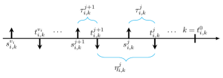
Figure 2: Illustration of the state parameters of plant $i$.

We introduce event-related time parameters in the following. Let $t_{i,k}^{j},j=1,2,\dots,v_{i}+1$, denote the time index of the $j$-th latest successful packet reception at actuator $i$ prior to the current time slot $k$, and $t_{i,k}^{0}\triangleq k$. Let $s_{i,k}^{j},j=0,\dots,v_{i}$, denote the time index of the latest successful sensor $i$’s transmission prior to $t_{i,k}^{j}$, where $s_{i,k}^{j}\leq t_{i,k}^{j}$, as illustrated in Fig 2.

Then, we define a sequence of variables, $\tau_{i,k}^{j},j=0,\dots,v_{i}$, as

$$\tau^{j}_{i,k}\triangleq t^{j}_{i,k}-s^{j}_{i,k},$$ (23)

to record the estimation quality at $k$ and at the $v_{i}$ successful control transmissions, where $\tau_{i,k}^{0}\triangleq\tau_{i,k}$ was defined above (11). Similarly, we define

$$\eta_{i,k}^{j}\triangleq t_{i,k}^{j}-t_{i,k}^{j+1},\quad j=0,\dots,v_{i},$$ (24)

denoting the time duration between consecutive successful controller’s transmissions, where $\eta_{i,k}^{0}\triangleq\eta_{i,k}$ was defined above (17). From (23) and (24), $\tau^{j}_{i,k}$ and $\eta^{j}_{i,k}$ can be treated as the AoI of the sensor’s and the controller’s packet of plant $i$, respectively, observed at $t_{i,k}^{j}$.

From (23), (11), (24), and (17), the updating rules of $\tau_{i,k}^{j}$ and $\eta_{i,k}^{j}$ can be obtained as

$$\tau_{i,k+1}^{j}=\begin{cases}\left.\begin{aligned} &1,&\mbox{ if }\beta_{i,k}=1\\ &\tau_{i,k}^{0}+1,&\mbox{ if }\beta_{i,k}=0\\ \end{aligned}\right\}\mbox{ for }j=0\\ \left.\begin{aligned} &\tau_{i,k}^{j-1},&\mbox{ if }\gamma_{i,k+1}=1\\ &\tau_{i,k}^{j},&\mbox{ if }\gamma_{i,k+1}=0\\ \end{aligned}\right\}\mbox{ for }j=1,\cdots,v_{i}\\ \end{cases}$$ (25)

$$\eta_{i,k}^{j}=\begin{cases}\left.\begin{aligned} &1,&\mbox{ if }\gamma_{i,k}=1\\ &\eta_{i,k-1}^{0}+1,&\mbox{ if }\gamma_{i,k}=0\\ \end{aligned}\right\}\mbox{ for }j=0\\ \left.\begin{aligned} &\eta_{i,k-1}^{j-1},&\mbox{ if }\gamma_{i,k}=1\\ &\eta_{i,k-1}^{j},&\mbox{ if }\gamma_{i,k}=0\\ \end{aligned}\right\}\mbox{ for }j=1,\cdots,v_{i}\\ \end{cases}$$ (26)

Now we define the AoI-related vector state of plant $i$ as

$$\mathbf{s}_{i,k}\triangleq(\tau_{i,k}^{0},\cdots,\tau_{i,k}^{v_{i}},\eta_{i,k}^{0},\cdots,\eta_{i,k}^{v_{i}}).$$ (27)

IV-B MDP Cost Function

We will show that the per-step cost function of plant $i$ in (22), i.e., $\mathbb{E}[\mathbf{x}^{\top}_{i,k}\mathbf{S}^{x}_{i}\mathbf{x}_{i,k}+\mathbf{u}^{\top}_{i,k}\mathbf{S}^{u}_{i}\mathbf{u}_{i,k}]$, is determined by the vector state $\mathbf{s}_{i,k}$. We focus on plant $i$ (the analytical method is identical for the other plants), and shall omit the plant index subscript of each parameter in the remainder of this subsection.

Taking (18) into (1), the plant state evolution can be rewritten as

$$\mathbf{x}_{k+1}=\mathbf{A}\mathbf{x}_{k}+\mathbf{B}\tilde{\mathbf{K}}(\mathbf{A}+\mathbf{B}\tilde{\mathbf{K}})^{\eta^{0}_{k}-1}\hat{\mathbf{x}}_{k+1-\eta^{0}_{k}}+\mathbf{w}_{k}.$$ (28)

By using this backward iteration for $k-t^{v}_{k}$ times and the definition of $\eta_{k}^{j}$ and $t^{j}_{k}$, we have

$$\mathbf{x}_{k}\!\!=\!\!(\mathbf{A}\!+\!\!\mathbf{B}\tilde{\mathbf{K}})^{\eta^{0}_{k}}\mathbf{x}_{t_{k}^{1}}\!\!+\!\!\big{(}\mathbf{A}^{\eta^{0}_{k}}\!\!-\!\!(\mathbf{A}\!+\!\mathbf{B}\tilde{\mathbf{K}})^{\eta^{0}_{k}}\big{)}\mathbf{e}_{t_{k}^{1}}\!\!+\!\!\!\sum_{i=1}^{\eta_{k}^{0}}\!\!\mathbf{A}^{i\!-\!1}\mathbf{w}_{k\!-i}$$ (29)

$$=(\mathbf{A}+\mathbf{B}\tilde{\mathbf{K}})^{\eta^{0}_{k}}\times$$

$$\bigg{(}\!\!(\mathbf{A}\!+\!\!\mathbf{B}\tilde{\mathbf{K}})^{\eta^{1}_{k}}\mathbf{x}_{t_{k}^{2}}\!\!+\!\big{(}\mathbf{A}^{\eta^{1}_{k}}\!-\!(\mathbf{A}\!+\!\mathbf{B}\tilde{\mathbf{K}})^{\eta^{1}_{k}}\big{)}\mathbf{e}_{t_{k}^{2}}\!+\!\!\sum_{i=1}^{\eta_{k}^{1}}\!\mathbf{A}^{i\!-\!1}\mathbf{w}_{t_{k}^{1}\!-\!i}\!\!\bigg{)}$$

$$+\big{(}\mathbf{A}^{\eta^{0}_{k}}-(\mathbf{A}+\mathbf{B}\tilde{\mathbf{K}})^{\eta^{0}_{k}}\big{)}\mathbf{e}_{t_{k}^{1}}+\sum_{i=1}^{\eta_{k}^{0}}\mathbf{A}^{i-1}\mathbf{w}_{k-i}$$

$$=\dots$$

$$=(\mathbf{A}+\mathbf{B}\tilde{\mathbf{K}})^{\eta_{k}^{0}+\eta_{k}^{1}+\cdots+\eta_{k}^{v-1}}\mathbf{x}_{t_{k}^{v}}+\mathbf{w}^{\prime}+\mathbf{e}^{\prime}$$

$$=\mathbf{w}^{\prime}+\mathbf{e}^{\prime},$$

where the last equation is due to the deadbeat control property (2). The quantity $\mathbf{w}^{\prime}$ is related to the plant disturbance and $\mathbf{e}^{\prime}$ is determined by the controller’s estimation errors at the successful control packet transmissions, i.e., $\mathbf{e}_{t^{1}_{k}},\dots,\mathbf{e}_{t^{v}_{k}}$, as given below:

$$\mathbf{w}^{\prime}=\sum_{i=1}^{\eta_{k}^{0}}\mathbf{A}^{i-1}\mathbf{w}_{k-i}+(\mathbf{A}+\mathbf{B}\tilde{\mathbf{K}})^{\eta_{k}^{0}}\sum_{i=1}^{\eta_{k}^{1}}\mathbf{A}^{i-1}\mathbf{w}_{k-i}+$$ (30)

$$\cdots+(\mathbf{A}+\mathbf{B}\tilde{\mathbf{K}})^{\eta_{k}^{0}+\cdots+\eta_{k}^{v-2}}\sum_{i=1}^{\eta_{k}^{v-1}}\mathbf{A}^{i-1}\mathbf{w}_{t_{k}^{v-1}-i}$$

$$=\sum_{j=1}^{v}\bigg{(}(\mathbf{A}+\mathbf{B}\tilde{\mathbf{K}})^{\sum_{m=0}^{j-2}\eta_{k}^{m}}\sum_{i=t_{k}^{j}}^{t_{k}^{j-1}-1}\mathbf{A}^{t_{k}^{j-1}-1-i}\mathbf{w}_{i}\bigg{)},$$ (31)

$$\mathbf{e}^{\prime}=\big{(}\mathbf{A}^{\eta_{k}^{0}}-(\mathbf{A}+\mathbf{B}\tilde{\mathbf{K}})^{\eta_{k}^{0}}\big{)}\mathbf{e}_{t_{k}^{1}}+$$ (32)

$$(\mathbf{A}+\mathbf{B}\tilde{\mathbf{K}})^{\eta_{k}^{0}}\big{(}\mathbf{A}^{\eta_{k}^{1}}-(\mathbf{A}+\mathbf{B}\tilde{\mathbf{K}})^{\eta_{k}^{1}}\big{)}\mathbf{e}_{t_{k}^{2}}+$$

$$\cdots+(\mathbf{A}\!+\!\mathbf{B}\tilde{\mathbf{K}})^{\eta_{k}^{0}+\cdots+\eta_{k}^{v-2}}\big{(}\mathbf{A}^{\eta_{k}^{v-1}}\!-\!(\mathbf{A}+\mathbf{B}\tilde{\mathbf{K}})^{\eta_{k}^{v-1}}\big{)}\mathbf{e}_{t_{k}^{v}}.$$ (33)

By analyzing the correlation between the sequences of plant disturbance and estimation noise, we have the following result.

Proposition 1.

The per-step cost function about the plant state is a deterministic function of the vector state $\mathbf{s}_{k}$ (see (27)) as

$$J^{x}(\mathbf{s}_{k})\triangleq\mathbb{E}\big{[}\mathbf{x}_{k}^{\top}\mathbf{S}^{x}\mathbf{x}_{k}\big{]}=\text{Tr}(\mathbf{S}^{x}V(\mathbf{s}_{k})),$$ (34)

where $V(\mathbf{s}_{k})\triangleq\mathbb{E}[\mathbf{x}_{k}\mathbf{x}^{\top}_{k}]$ is the plant state covariance given in (36). In the latter equation, for $0\leq i\leq j\leq v$, we have

$$\Delta_{k}(i,j)\triangleq s_{k}^{i}-s_{k}^{j}=\sum_{n=i}^{j-1}\eta_{k}^{n}+\tau_{k}^{j}-\tau_{k}^{i}.$$ (35)

$$V(\mathbf{s}_{k}) =\mathbf{D}_{k}\hat{\mathbf{P}}^{s}(\mathbf{D}_{k})^{\top}+\sum_{n=1}^{v-1}\big{(}\sum_{i=0}^{\Delta_{k}(n,n+1)-1}\check{\mathbf{E}}_{(k,n)}^{i}\mathbf{Q}_{w}(\check{\mathbf{E}}_{(k,n)}^{i})^{\top}\big{)}+\sum_{i=0}^{\eta_{k}^{0}+\tau_{k}^{1}-1}\mathbf{A}^{i}\mathbf{Q}_{w}(\mathbf{A}^{i})^{\top}+\sum_{n=1}^{v-1}\big{(}\sum_{i=0}^{\Delta_{k}(n,n+1)-1}\check{\mathbf{F}}^{i}_{(k,n)}\mathbf{Q}_{v}(\check{\mathbf{F}}^{i}_{(k,n)})^{\top}\big{)},$$ (36)

$$\mathbf{D}_{k} \triangleq\sum_{j=1}^{v}\bigg{(}(\mathbf{A}+\mathbf{B}\tilde{\mathbf{K}})^{\sum_{m=0}^{j-2}\eta_{k}^{m}}\big{(}\mathbf{A}^{\eta_{k}^{j-1}}-(\mathbf{A}+\mathbf{B}\tilde{\mathbf{K}})^{\eta_{k}^{j-1}}\big{)}\mathbf{A}^{\tau_{k}^{j}}\mathbf{Z}^{\Delta_{k}(j,v)}\bigg{)},$$

$$\check{\mathbf{E}}_{(k,n)}^{i} \triangleq(\mathbf{A}+\mathbf{B}\tilde{\mathbf{K}})^{\sum_{m=0}^{n-1}\eta_{k}^{m}}\mathbf{A}^{\tau_{k}^{n}+i}+\sum_{j=1}^{n}\bigg{(}(\mathbf{A}+\mathbf{B}\tilde{\mathbf{K}})^{\sum_{m=0}^{j-2}\eta_{k}^{m}}\big{(}\mathbf{A}^{\eta_{k}^{j-1}}-(\mathbf{A}+\mathbf{B}\tilde{\mathbf{K}})^{\eta_{k}^{j-1}}\big{)}\mathbf{A}^{\tau_{k}^{j}}\mathbf{Z}^{i+\Delta_{k}(j,n)}(\mathbf{I}-\hat{\mathbf{K}}\mathbf{C})\bigg{)},$$

$$\check{\mathbf{F}}^{i}_{(k,n)} \triangleq\sum_{j=1}^{n}\bigg{(}(\mathbf{A}+\mathbf{B}\tilde{\mathbf{K}})^{\sum_{m=0}^{j-2}\eta_{k}^{m}}\big{(}\mathbf{A}^{\eta_{k}^{j-1}}-(\mathbf{A}+\mathbf{B}\tilde{\mathbf{K}})^{\eta_{k}^{j-1}}\big{)}\mathbf{A}^{\tau_{k}^{j}}\mathbf{Z}^{\Delta_{k}(j,n)+i}\hat{\mathbf{K}}\bigg{)}$$

Then, building on the system dynamics (1), the local estimate (4), the remote estimate (9), and the control input (18), and by comprehensively analyzing the effect of the correlations between plant disturbance and estimation noise on the control input covariance, we obtain the per-step cost function about the control input as below.

Proposition 2.

The per-step cost function about the control input at $k$ is a deterministic function of the vector state $\mathbf{s}_{k}$ as

$$J^{u}(\mathbf{s}_{k})\triangleq\mathbb{E}\big{[}\mathbf{u}_{k}^{\top}\mathbf{S}^{u}\mathbf{u}_{k}\big{]}$$ (37)

$$=\!\!\text{Tr}\bigg{(}\!\!\big{(}\tilde{\mathbf{K}}(\!\mathbf{A}\!+\!\mathbf{B}\tilde{\mathbf{K}}\!)^{\eta_{k}\!-\!1}\big{)}^{\!\!\top}\!\mathbf{S}^{u}\big{(}\tilde{\mathbf{K}}(\!\mathbf{A}\!+\!\mathbf{B}\tilde{\mathbf{K}}\!)^{\eta_{k}\!-\!1}\big{)}\hat{V}(\mathbf{s}_{k+1-\eta_{k}})\!\!\bigg{)},$$

where $\mathbf{s}_{k+1-\eta_{k}}$ can be directly obtained by $\mathbf{s}_{k}$. $\hat{V}(\mathbf{s}_{k})\triangleq\mathbb{E}[\hat{\mathbf{x}}_{k}\hat{\mathbf{x}}_{k}^{\top}]$ is the covariance of the remote estimate given in (41), where

$$\tilde{\mathbf{D}}_{k}\ \triangleq\mathbf{D}_{k}-\mathbf{A}^{\tau_{k}^{0}}\mathbf{Z}^{\Delta_{k}(0,v)},$$ (38)

$$\dot{\mathbf{E}}_{(k,n)}^{i} \triangleq\check{\mathbf{E}}_{(k,n)}^{i}-\mathbf{A}^{\tau_{k}^{0}}\mathbf{Z}^{\Delta_{k}(0,n)-\tau_{k}^{n}+i}(\mathbf{I}-\hat{\mathbf{K}}\mathbf{C}),$$ (39)

$$\dot{\mathbf{F}}_{(k,n)}^{i} \triangleq\check{\mathbf{F}}_{(k,n)}^{i}+\mathbf{A}^{\tau_{k}^{0}}\mathbf{Z}^{\Delta_{k}(0,n)+i}\hat{\mathbf{K}}.$$ (40)

$$\hat{V}(\mathbf{s}_{k})=\tilde{\mathbf{D}}_{k}\hat{\mathbf{P}}^{s}\tilde{\mathbf{D}}_{k}^{\top}\!\!+\!\!\sum_{n=1}^{v-1}\big{(}\sum_{i=0}^{\Delta_{k}(n,n+1)-1}\dot{\mathbf{E}}_{(k,n)}^{i}\mathbf{Q}_{w}(\dot{\mathbf{E}}_{(k,n)}^{i})^{\top}\big{)}+\!\!\!\!\!\!\!\!\sum_{i=0}^{\Delta_{k}(0,1)-1}\!\!\big{(}\mathbf{A}^{\tau_{k}^{0}+i}-\mathbf{A}^{\tau_{k}^{0}}\mathbf{Z}^{i}(\mathbf{I}-\hat{\mathbf{K}}\mathbf{C})\big{)}\mathbf{Q}_{w}\big{(}\mathbf{A}^{\tau_{k}^{0}+i}-\mathbf{A}^{\tau_{k}^{0}}\mathbf{Z}^{i}(\mathbf{I}-\hat{\mathbf{K}}\mathbf{C})\big{)}^{\top}$$ (41)

$$\quad\qquad+\sum_{n=1}^{v-1}\big{(}\sum_{i=0}^{\Delta_{k}(n,n+1)-1}\dot{\mathbf{F}}_{(k,n)}^{i}\mathbf{Q}_{w}(\dot{\mathbf{F}}_{(k,n)}^{i})^{\top}\big{)}+\sum_{i=0}^{\Delta_{k}(0,1)-1}\big{(}\mathbf{A}^{\tau_{k}^{0}}\mathbf{Z}^{i}\hat{\mathbf{K}}\big{)}\mathbf{Q}_{w}\big{(}\mathbf{A}^{\tau_{k}^{0}}\mathbf{Z}^{i}\hat{\mathbf{K}}\big{)}^{\top}$$

The proofs of Propositions 1 and 2 are given in Appendices B and C, respectively.

Remark 3.

From Propositions 1 and 2, the per-step cost of the plant is determined by the finite-length vector state $\mathbf{s}_{k}$. However, expressions for the cost functions are involved due to the sequential predictive control and the command buffer adopted at the actuator, as well as the consideration of plant disturbance, and local and remote estimation errors.

By substituting plant index $i$ into the vector state and the cost functions (34) and (37), the above results have opened the door to address the optimal scheduling problem of the $N$-plant-$M$-frequency WNCS with ETDC in (22) as a decision making problem with a countable state space.

IV-C Resulting MDP

From (19), (25) and (26), given the current state $\mathbf{s}_{i,k}$ and the current transmission scheduling action related to plant $i$, the next state, $\mathbf{s}_{i,k+1}$, is independent of all previous states and actions, satisfying the Markov property. Thus, the transmission scheduling problem of the WNCS can be formulated as an MDP:

• The state of the MDP at time $k$ is $\mathbf{s}_{k}\triangleq(\mathbf{s}_{1,k},\cdots,\mathbf{s}_{N,k})$, where $\mathbf{s}_{i,k}$ is as defined in (27), $i=1,\dots,N$. The state space is $\mathcal{S}=\underbrace{\mathbb{N}^{2v_{1}+2}\times\cdots\times\mathbb{N}^{2v_{N}+2}}_{N\;\text{terms}}$.

• The action at time $k$, $\mathbf{a}_{k}\triangleq[a_{1,k},a_{2,k},\dots,a_{M,k}]=\pi(\mathbf{s}_{k})$, is the transmission link allocation at each frequency, where $a_{m,k}\in\{-N,\dots,N\},\ m=1,\dots,M$, and ${a}_{m,k}\neq{a}_{m^{\prime},k}$ if ${a}_{m,k}{a}_{m^{\prime},k}\neq 0$. Then, the action space $\mathcal{A}\subseteq\{-N,\dots,N\}^{M}$ has the cardinality of $|\mathcal{A}|=\sum_{m=0}^{M}\mathsf{C}^{m}_{M}\mathsf{P}^{m}_{2N}$.

• The state transition probability $P(\mathbf{s}_{k+1}|\mathbf{s}_{k},\mathbf{a}_{k})$ can be obtained directly from the state updating rules in (19), (25) and (26).

• The per-step cost of the MDP is the sum cost of each plant in Propositions 1 and 2 as

  $$c(\mathbf{s}_{k})\triangleq\sum_{i=1}^{N}c_{i}(\mathbf{s}_{i,k}),$$ (42)

  where $c_{i}(\mathbf{s}_{i,k})\triangleq J^{x}_{i}(\mathbf{s}_{i,k})+J^{u}_{i}(\mathbf{s}_{i,k})$.

• The discount factor is $\vartheta\in(0,1)$.

• The scheduling problem of the $N$-plant-$M$-frequency system can be rewritten as

  $$\min_{\pi}\mathbb{E}^{\pi}\left[\sum_{k=0}^{\infty}\vartheta^{k}c(\mathbf{s}_{k})\right].$$ (43)

Remark 4.

The discounted MDP problem above with an infinite state space can be numerically solved to some extent by using classic policy or value iteration methods with a truncated state space $\mathcal{S}_{L}$

$$\mathcal{S}_{L}\triangleq\underbrace{\mathbb{N}_{L}^{2v_{1}+2}\times\cdots\times\mathbb{N}_{L}^{2v_{N}+2}}_{N\;\textrm{terms}},\text{where }\mathbb{N}_{L}=\{1,\dots,L\}.$$ (44)

The computation complexity of relative value iteration algorithm is given as $\mathcal{O}(|\mathcal{S}_{L}||\mathcal{A}|^{2}K)$ [28], where $K$ is the number of iteration steps, and the state space and action space sizes are $|\mathcal{S}|=L^{2\sum_{i=1}^{N}v_{i}+2N}$ and $|\mathcal{A}|=\sum_{m=0}^{M}\mathsf{C}^{m}_{M}\mathsf{P}^{m}_{2N}$, respectively. However, the sizes of both the state and action spaces are considerably large even for relatively small $N$ and $M$, leading to numerical difficulties in finding a solution. In the literature of WNCS, even for the (simpler) $N$-plant-$M$-channel remote estimation system, only the $M=1$ case has been found to have a numerical solution [7]. To tackle the challenge for larger scale WNCS deployment, we will use DRL methods exploiting deep neural networks for function approximation in the following.

Remark 5.

Although the MDP problem formulation of the WNCS assumes static wireless channels with fixed packet drop probabilities, it can be extended to a Markov fading channel scenario. A Markov fading channel can have multiple channel states with different packet drop probabilities, and the channel state transition is modeled by a Markov chain [22]. In this scenario, the state of the MDP problem should also include the channel state, and the state transition probability needs to take into account both the AoI state and the Markov channel state transition probabilities. The details of WNCS scheduling over Markov fading channels can be investigated in our future work.

V WNCS Scheduling with Deep Reinforcement Learning

Building on the MDP framework, DRL is widely applied in solving decision making problems with pre-designed state space, action space, per-step reward (cost) function and discount factor for achieving the maximum long-term reward. The main difference is that DRL does not exploit the state transition probability as required by MDP, but records and utilizes many sampled data sequences, including the current state $\mathbf{s}$, action $\mathbf{a}$, reward $r$ and next state $\mathbf{s}^{\prime}$, to train deep neural networks for generating the optimal policy [29]. To find deterministic policies, the most widely considered DRL algorithms are deep deterministic policy gradient (DDPG) [30] and deep Q-learning [31], where the former and the latter work for continuous and discrete action spaces, respectively. We choose deep Q-learning, since the action space $\mathcal{A}$ in our problem (Section IV-C) is finite. In general, we consider an episodic training scenario, where the system is operating in a simulated environment. Hence, one can learn and gather samples over multiple episodes to train a policy. Then, after verifying the properties of the final policy, one can “safely” deploy it [30]. We note that if the DRL policy does lead to instability (i.e., an unbounded expected cost), one needs to adjust the hyperparameters of the deep neural network (e.g., the initial network parameters and the number of layers and neurons) and start retraining. Such readjusting of hyperparameters of a deep learning agent is commonly adopted in practice [31].

In the following, we present a deep-Q-learning approach for scheduler design that requires a sampled data sequence $\{(\mathbf{s,a},r,\mathbf{s^{\prime}})\}$. We note that the data sampling and the deep Q-learning are conducted offline. In particular, given the current state and action pair $(\mathbf{s,a})$, the reward $r$ can be obtained immediately from Propositions 1 and 2, and the next state $\mathbf{s}^{\prime}$ affected by the scheduling action and the packet dropouts can be sampled easily based on the packet error probabilities of each channel (19) and state transition rules (25) and (26). Furthermore, the trained policy needs to be tested offline to verify the WNCS’s stability before an online deployment.

V-A Deep Q-Learning Approach

We introduce the state-action value function given a policy $\pi(\cdot)$, which is also called the $Q$ function [13]:

$$Q^{\pi}(\mathbf{s,a})\!\triangleq\!\mathbb{E}\left[\sum_{k=0}^{\infty}\vartheta^{k}r_{k}|\mathbf{s}_{0}=\!\mathbf{s},\mathbf{a}_{0}=\!\mathbf{a},\mathbf{a}_{k}=\!\pi(\mathbf{s}_{k}),\forall k>0\right]\!,$$ (45)

where $r_{k}\triangleq-c(\mathbf{s}_{k})$ can be treated as the negative cost function in (42) at $k$. Then, by dropping out the time index $k$, the $Q$ function of the maximum average discounted total reward achieving policy $\pi^{\star}(\cdot)$ satisfies the Bellman equation as

$$Q^{\star}(\mathbf{s,a})=\mathbb{E}\big{[}r+\vartheta\max_{\mathbf{a}^{\prime}\in\mathcal{A}}Q^{\star}(\mathbf{s^{\prime},a^{\prime}})|\mathbf{s,a}\big{]}.$$ (46)

The optimal stationary and deterministic policy can be written as

$$\mathbf{a}^{\star}=\pi^{\star}(\mathbf{s})\triangleq\arg\max_{\mathbf{a}\in\mathcal{A}}Q^{\star}(\mathbf{s,a}).$$ (47)

Solving the optimal $Q$ function is the key to find the optimal policy, but is computationally intractable by conventional methods as discussed in Remark 4. In contrast, deep Q-learning methods approximate $Q^{\star}(\mathbf{s,a})$ by a function $Q(\mathbf{s,a};\theta)$ parameterized by a set of neural network parameters, $\theta$, (including both weights and biases), and then learns $\theta$ to minimize the difference between the left- and right-hand sides of (46) [14]. Deep Q-learning can be easily implemented by the most well-known machine learning framework TensorFlow with experience replay buffer, $\epsilon$-greedy exploration and mini-batch sampling techniques [32]. Building on this, the approach for solving problem (43) is given as Algorithm 1.

1:Initialize experience replay buffer $\mathcal{B}$ to capacity $K$

2:Initialize multi-layer fully connected neural network $Q$ with vector input $\mathbf{s}$, $|\mathcal{A}|$ outputs $\{Q(\mathbf{s},\mathbf{a}_{1};\theta_{0}),\dots,Q(\mathbf{s},\mathbf{a}_{|\mathcal{A}|};\theta_{0})\}$ and random parameter set $\theta_{0}$

3:for episode = $1,\cdots,E$ do

4:     Randomly initialize $\mathbf{s}_{0}$

5:     for $t=0,1,\cdots,T$ do

6:         With probability $\epsilon$ select a random action $\mathbf{a}_{t}$, otherwise select $\mathbf{a}_{t}=\arg\max_{\mathbf{a}\in\mathcal{A}}Q(\mathbf{s}_{t},\mathbf{a};\theta_{t})$

7:         Execute $\mathbf{a}_{t}$ , and obtain $r_{t}$ and $\mathbf{s}_{t+1}$

8:         Store $(\mathbf{s}_{t},\mathbf{a}_{t},r_{t},\mathbf{s}_{t+1})$ in $\mathcal{B}$

9:         Sample random mini-batch of $l$ transitions $(\mathbf{s}_{t},\mathbf{a}_{t},r_{t},\mathbf{s}_{t+1})$ from $\mathcal{B}$ as $\tilde{\mathcal{B}}$

10:         Set $z_{j}=r_{j}+\vartheta\max_{\mathbf{a}^{\prime}\in\mathcal{A}}\hat{Q}(\mathbf{s}_{j+1},\mathbf{a}^{\prime};\theta_{t})$ for each sample in $\tilde{\mathcal{B}}$

11:         Perform a mini-batch gradient descend step to minimize the Bellman error, i.e., $\min_{\hat{\theta}}\sum_{\tilde{\mathcal{B}}}(z_{j}-Q(\mathbf{s}_{j},\mathbf{a}_{j};\hat{\theta}))^{2}$

12:         Update $\theta_{t+1}=\hat{\theta}$

13:     end for

14:end for

Algorithm 1 Deep Q-learning for transmission scheduling in WNCS

V-B Deep Q-Learning with Reduced Action Space

In practice, the training of deep Q-network (DQN) converges and the trained DQN performs well for simple decision-making problems with a bounded reward function, small input state dimension and small action space, see e.g., [32], where the state input is a length-$4$ vector and there are only $2$ possible actions. However, for the problem of interest in the current work, the reward function is unbounded (due to the potential of consecutive packet dropouts), the state $\mathbf{s}$ is of high dimension, and action-space $|\mathcal{A}|$ is large. Hence, the convergence of the DQN training is not guaranteed for all hyper-parameters, which include the initialization of $\theta$, the number of neural network layers, the number of neurons per layer, and the reply buffer and mini-batch sizes. Even if the convergence is achieved, due to the complexity of the problem, it may take very long training time and only converge to a local optimal parameter set $\theta$ (which is also affected by the choice of hyper-parameters), leading to a worse performance than some conventional scheduling policies. Whilst the hyper-parameters can in principle be chosen to enhance performance, no appropriate tuning guidelines exist for the problem at hand.

To overcome the computational issues outlined above, in the following we will reduce the action space. This will make the training task simpler and enhance the convergence rate. To be more specific, for each plant system, instead of considering all the possible actions to schedule either or both of the uplink and downlink communications at each time instant, we restrict to the two modes downlink only and uplink only. Switching between these two modes of operation occurs once a scheduled transmission of that plant is successful.

The principle behind this is the intuition that the controller requires the information from the sensor first and then performs control, and so on and so forth. The above concept can be incorporated into the current framework by adding the downlink/uplink indicator $s^{\text{link}}_{i,k}\in\{-1,1\},\forall i=1,\dots,N$, into state $\mathbf{s}_{k}$ leading to the aggregated state

$$\breve{\mathbf{s}}_{k}\triangleq[\mathbf{s}_{k},s^{\text{link}}_{1,k},\dots,s^{\text{link}}_{N,k}],$$

where $s^{\text{link}}_{i,k}=1$ or $-1$ indicates the uplink or downlink of plant $i$ can be scheduled at $k$. The state updating rule is

$$s^{\text{link}}_{i,k+1}=\begin{cases}-1&\text{ if }s^{\text{link}}_{i,k}=1\text{ and }\beta_{i,k}=1\\ 1&\text{ if }s^{\text{link}}_{i,k}=-1\text{ and }\gamma_{i,k}=1\\ s^{\text{link}}_{i,k}&\text{ otherwise.}\\ \end{cases}$$ (48)

The new scheduling action at the $M$ frequencies is denoted as $\breve{\mathbf{a}}_{k}\triangleq[\breve{a}_{1,k},\dots,\breve{a}_{M,k}]$, where $\breve{a}_{m,k}\in\{0,\dots,N\},\;\forall m\in\{1,\dots,M\}$, and $\breve{a}_{m,k}\neq\breve{a}_{m^{\prime},k}$ if $\breve{a}_{m,k}\breve{a}_{m^{\prime},k}\neq 0$. If $\breve{a}_{m,k}=i$ and $s^{\text{link}}_{i,k}=1$, then the uplink of plant $i$ is scheduled on frequency $m$ at time $k$. Compared with the original action $\mathbf{a}_{k}$ in Section IV-C, the size of the new action space is reduced significantly to $|\tilde{\mathcal{A}}|=\sum_{m=0}^{M}\mathsf{C}^{m}_{M}\mathsf{P}^{m}_{N}$. For example, when $N=3$, $M=3$ and $v_{1}=v_{2}=v_{3}=2$, the action space size is reduced from $229$ to $34$. By replacing $\mathbf{s}$ and $\mathbf{a}$ with $\breve{\mathbf{s}}$ and $\breve{\mathbf{a}}$, respectively, in Algorithm 1, we can apply the deep Q-learning method to find a policy with a reduced action space at a faster rate.

We will illustrate numerical results of using deep Q-learning for solving the action-space-reduced problem in the following section.

VI Numerical Results

We first consider a $N$-plant-$M$-frequency WNCS with $N=3$ and $M=3$, i.e., $6$ links sharing $3$ frequencies. Then, we will extend the network to a larger scale. The plant system matrices are

$$\mathbf{A}_{1}=\begin{bmatrix}1.1&0.2\\ 0.2&0.8\end{bmatrix},\;\mathbf{A}_{2}=\begin{bmatrix}1.2&0.2\\ 0.2&0.9\end{bmatrix},\;\mathbf{A}_{3}=\begin{bmatrix}1.3&0.2\\ 0.2&1.0\end{bmatrix},$$

in which case $\rho(\mathbf{A}_{1})=1.2$, $\rho(\mathbf{A}_{2})=1.3$ and $\rho(\mathbf{A}_{3})=1.4$. The control input matrices are all set to $\mathbf{B}_{i}=[1\ 1]^{\top},i=1,2,3$. The measurement matrix $\mathbf{C}_{i},i=1,2,3$ is equal to the identity matrix. The covariance matrices are $\mathbf{Q}^{w}_{i}=\mathbf{Q}^{v}_{i}=0.1\mathbf{I}$, $i=1,2,3$.

Each plant is $2$-step controllable, i.e., $v_{i}=2,i=1,2,3$, and the deadbeat control gains of each plant are given as $\mathbf{K}_{1}=[-2.90,1.00],\mathbf{K}_{2}=[-3.533,1.433],\mathbf{K}_{3}=[-4.233,1.933]$. The packet success probabilities of each link, i.e., $\xi^{s}_{m,i}$ and $\xi^{c}_{m,i}$, $i,m=1,2,3$, are generated randomly and drawn uniformly from $(0.65,1.0)$. The resulting WNCS satisfies the stability condition established in Theorem 1.

The weighting terms $\mathbf{S}^{x}_{i}$ and $\mathbf{S}^{u}_{i}$ are chosen as identity matrices and the discount factor is $\vartheta=0.95$. We adopt the following hyper-parameters deep Q-learning. The input state dimension of DQN is set to $2N(v+1)=18$, i.e., the input layer has $18$ neurons. We use one hidden layer with $1024$ neurons, and an output layer with $34$ outputs (actions) for the problem with reduced action space (see Section V-B). The activation function in the hidden layer is the ReLU [32]. The experience reply memory has size of $K=20000$, and the size of mini-batch is $32$. So in each time step, $32$ data is sampled from the reply memory for training. The exploration parameter $\epsilon$ decreases from $1$ to $0.01$ at the rate of $0.999$ after each time step. We adopt the ADAM optimizer in solving the optimization problem in Step 11 of Algorithm 1. Each DQN-training takes $E=1000$ episodes, each including $T=500$ time steps. We test the trained policy for $1000$ episodes and compare the empirical average costs $\frac{1}{T}\sum_{k=1}^{T}c(\mathbf{s}_{k})$.

We use Algorithm 1 to solve the scheduling problem with reduced action space and compare it with three benchmark policies. 1) Random policy: randomly choose $M$ out of the $2N$ links and randomly allocate them to the $M$ frequencies at each time. 2) Round-robin policy: the $2N$ links are divided into $M$ groups, and the links in each of the groups $m\in\{1,\dots,M\}$ are allocated to the corresponding frequency $m$; the transmission scheduling at each frequency follows the round-robin fashion [15] at each time. Note that in the simulation, we test all link-grouping combinations and only present the one with the lowest average cost. 3) Greedy policy: At each time, the $M$ frequencies are allocated to $M$ of the $2N$ links with the largest AoI value in $\{\tau_{1,k},\eta_{1,k},\dots,\tau_{N,k},\eta_{N,k}\}$. Recall that $\tau_{i,k}$ and $\eta_{i,k}$ denote the time duration since the last received sensing and control packets of plant $i$, respectively. The link with the highest AoI value chooses the frequency channel first with the highest packet success probability; then the link with the second highest value selects from the rest of the frequencies, and so on.

In Fig. 3, we show the (per-episode) empirical average cost during DQN training process with $1000$ episodes, and also the testing results (empirical average cost) of the trained DQN and the benchmark policies. We see that the training process converges quickly at about $100$ episodes, and the trained DQN-based policy reduces the empirical average cost of the best benchmark policy (greedy policy) by $42.5\%$, from $20$ to $11.5$.

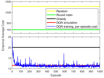
Figure 3: Empirical average cost over different traning episodes. Also included are the long term average performance of other benchmark algorithms.

We also randomly generate another $10$ different wireless channel conditions (packet success probabilities), train DQN for each set up and present the simulating results of the DQN-based policy and benchmark policies in Table I. The results show that the DQN-based policy can at least reduce the average cost by $25\%$ compared with the benchmark policies, verifying the effectiveness of the proposed DQN-based approach.

In Table II, we have extended the setup to a $6$-plant-$4$-channel scenario, where the size of the hidden layers of the DQN is doubled compared to the $3$-plant-$3$-channel scenario, and the output layer has $1045$ neurons. The 6 plant system matrices are $\mathbf{A}_{1}$, $\mathbf{A}_{1}$, $\mathbf{A}_{2}$, $\mathbf{A}_{2}$, $\mathbf{A}_{3}$ and $\mathbf{A}_{3}$, respectively, where $\mathbf{A}_{1}$, $\mathbf{A}_{2}$, and $\mathbf{A}_{3}$ are defined at the beginning of this section. We see that the DQN algorithm can achieve a $25\%$ to $35\%$ average cost reduction compared with the best of the benchmark policies examined. Also, the average cost of the $6$-plant-$4$-channel scenario is more than twice larger than the $3$-plant-$3$-channel scenario. This is because the former has less wireless channels per plant than the latter.

TABLE I: Empirical average costs for ten randomly generated wireless channel conditions with $N=3$ and $M=3$.

Experiment	Random	Round robin	Greedy	DQN
1	1385.6	19.4	19.2	11.3
2	1268.9	13.9	18.9	10.4
3	705.5	68.1	19.8	13.3
4	6185.4	40.3	19.9	12.9
5	3325.2	15.7	16.6	11.3
6	133.8	13.8	14.7	10.5
7	26221.4	94.8	22.9	15.9
8	702.0	23.3	16.5	10.5
9	1966.9	14.3	18.3	10.6
10	262.2	12.2	16.2	9.1

TABLE II: Empirical average costs for ten randomly generated wireless channel conditions with $N=6$ and $M=4$.

Experiment	Random	Round robin	Greedy	DQN
1	207056.9	102.1	72.1	49.2
2	526059.4	317.5	79.3	58.7
3	756337.2	202.3	79.4	54.1
4	139596.4	202.5	69.3	48.7
5	1551247.7	251.7	75.6	56.1
6	216834.3	429.1	89.2	65.0
7	4004723.8	135.2	77.2	54.7
8	1139943.9	222.0	67.5	45.8
9	68021277.2	118.5	69.9	47.3
10	2725231.0	647.1	86.8	64.1

VII Conclusions

We have investigated the transmission scheduling problem of the fully distributed WNCS. A sufficient stability condition of the WNCS in terms of both the control and communication system parameters has been derived. We have proposed a reduced-complexity DRL algorithm to solve the scheduling problem, which performs much better than benchmark policies. For future work, we will develop a distributed DRL approach for enhancing the scalability of the scheduling algorithm. Furthermore, we will consider co-design problems of the estimator, the controller, and the scheduler for distributed WNCSs with time-varying channel conditions.

Appendix A Proof of Theorem 1

Proof of (a). We focus on the mean-square stability condition analysis of plant $i$, which is assumed to be allocated to frequency $m$. The stability condition of the other plants can be obtained in the same way.

We introduce the concept of stochastic control cycle, which divides the infinite time domain into effective control cycles. Each control cycle of plant $i$ starts after the completion of $v_{i}$ step control and ends in the next completion, as illustrated below:

$$\{\!\cdots\overbrace{\underbrace{\text{o}\cdots\text{o}}_{l^{o}_{i,t-1}}\underbrace{\text{s}\cdots\text{s}}_{l^{s}_{i,t-1}}\underbrace{\text{c}\cdots\text{c}}_{l^{c}_{i,t-1}}\underbrace{\text{v}\cdots\text{v}}_{l^{v}_{i,t-1}}}^{\text{control cycle }(t-1)}\overbrace{\underbrace{\text{o}\cdots\text{o}}_{l^{o}_{i,t}}\underbrace{\text{s}\cdots\text{s}}_{l^{s}_{i,t}}\underbrace{\text{c}\cdots\text{c}}_{l^{c}_{i,t}}\underbrace{\text{v}\cdots\text{v}}_{l^{v}_{i,t}}}^{\text{control cycle }t}\cdots\!\},$$ (49)

where ‘o’, ‘s’, ‘c’ and ‘v’ stages denote the other plants’ (within $\mathcal{F}_{m}$) transmission scheduling, the uplink scheduling of plant $i$, the downlink scheduling of plant $i$ and the control command execution, respectively.

Since the instability is caused by the potential infinite consecutive packet dropouts, the fixed $v_{i}-1$ step deadbeat control won’t affect the instability. In the following, for ease of clarification but without loss of generality, we work on the $v_{i}=1$ case, i.e., the control cycles do not contains the ‘v’ stage. The stability conditions of the $v_{i}>1$ cases can be proved in a similar way and have the same result as $v_{i}=1$. Without loss of generality, we assume that the first control cycles starts at $k=1$. Let $t$ be the control cycle index, $L_{i,t}$ be the length of the $t$th cycle, and define the total cost in cycle $t$ of plant $i$ as

$$C_{i,t}\triangleq\sum_{k=\sum_{t^{\prime}=1}^{t-1}L_{t^{\prime}}+1}^{\sum_{t^{\prime}=1}^{t}L_{t^{\prime}}}\tilde{c}_{i,k},t=1,2,\dots.$$ (50)

where $\tilde{c}_{i,k}\triangleq\mathbf{x}_{i,k}^{\top}\mathbf{x}_{i,k}$, and hence

$$\mathbb{E}[\tilde{c}_{i,k}]=\text{Tr}(\mathbf{P}_{i,k}),$$ (51)

and $\mathbf{P}_{i,k}\triangleq\mathbb{E}[\mathbf{x}_{i,k}\mathbf{x}^{\top}_{i,k}]$.

From [22, page 6], it directly follows that the average cost is bounded if the average sum cost per cycle is. Thus, in the following, we merely need to derive a condition which ensures that $\mathbb{E}[C_{i,t}]<\infty,\forall t=1,2\dots.$

We derive the average sum cost of the first control cycle. Since the plant states are not affected by any control input within the first control cycle, from (1), it follows that:

$$\mathbb{E}[\tilde{c}_{i,k}]=\text{Tr}\left(g^{k-1}_{i}(\mathbf{P}_{i,1})\right)<\zeta_{i}(\rho^{2}(\mathbf{A}_{i})+\varepsilon_{i})^{k},$$ (52)

where $\mathbf{P}_{i,1}$ is bounded due to Assumption 1,

$$g^{0}_{i}(\mathbf{X})=\mathbf{X},g^{1}_{i}(\mathbf{X})=g_{i}(\mathbf{X})\triangleq\mathbf{A}_{i}\mathbf{X}\mathbf{A}^{\top}_{i}+\mathbf{Q}^{w}_{i},$$ (53a)

$$g^{j+1}_{i}(\cdot)=g_{i}(g^{j}_{i}(\cdot)),$$ (53b)

and $\zeta_{i}$ is a positive constant, $\varepsilon_{i}$ can be any arbitrary small positive number, and the inequality is based on [22, Proposition 1].

Using (50) and (52), the conditional average sum cost in the first control cycle is

$$\mathbb{E}[C_{i,1}|L_{i,1}\!\!=\!l_{i,1}]\!\!<\!\!\!\begin{cases}l_{i,1}\zeta_{i}\left(\rho^{2}(\mathbf{A}_{i})\!+\!\varepsilon_{i}\right)^{l_{i,1}}\!\!\!,&\text{\!\!\!\!\!\! if }(\rho^{2}(\mathbf{A}_{i})\!+\!\varepsilon_{i})\!\!\geq\!\!1\\ l_{i,1}\zeta_{i}\left(\rho^{2}(\mathbf{A}_{i})\!+\!\varepsilon_{i}\right),&\text{\!\!\!\!\!\! otherwise.}\end{cases}$$ (54)

Using the i.i.d. packet dropout assumption in Section II-E, the average sum cost for the $(\rho^{2}(\mathbf{A}_{i})+\varepsilon_{i})\geq 1$ case can be obtained as

$$\mathbb{E}[C_{i,1}]=\!\!\sum_{l_{i,1}=1}^{\infty}\mathbb{P}[L^{o}_{i,1}+L^{s}_{i,1}+L^{c}_{i,1}\!=\!l_{i,1}]\mathbb{E}[C_{i,1}|L_{i,1}=l_{i,1}]$$ (55)

$$=\sum_{l^{o}_{i,1}=1}^{\infty}\sum_{l^{s}_{i,1}=1}^{\infty}\sum_{l^{c}_{i,1}=1}^{\infty}\mathbb{P}[L^{o}_{i,1}=l^{o}_{i,1}]\mathbb{P}[L^{s}_{i,1}=l^{s}_{i,1}]\mathbb{P}[L^{c}_{i,1}=l^{c}_{i,1}]$$

$$\hskip 108.12054pt\times\mathbb{E}[C_{i,1}|L_{i,1}=l^{o}_{i,1}+l^{s}_{i,1}+l^{c}_{i,1}]$$

$$<\sum_{l^{o}_{i,1}=1}^{\infty}\sum_{l^{s}_{i,1}=1}^{\infty}\sum_{l^{c}_{i,1}=1}^{\infty}\mathbb{P}[L^{o}_{i,1}=l^{o}_{i,1}]\mathbb{P}[L^{s}_{i,1}=l^{s}_{i,1}]\mathbb{P}[L^{c}_{i,1}=l^{c}_{i,1}]$$

$$\hskip 142.26378pt\times l_{i,1}\zeta_{i}\left(\rho^{2}(\mathbf{A}_{i})+\varepsilon_{i}\right)^{l_{i,1}}$$

where $L^{o}_{i,j}$, $L^{s}_{i,j}$ and $L^{c}_{i,j}$ denote the length of the ‘o’, ‘s’ and ‘c’ stages in the $j$th cycle of plant $i$, with realizations $l^{o}_{i,j}$, $l^{s}_{i,j}$ and $l^{c}_{i,j}$, respectively, and $L_{i,j}=L^{o}_{i,j}+L^{s}_{i,j}+L^{c}_{i,j}$. Since $\mathbb{P}[L^{c}_{i,1}=l^{c}_{i,1}]=\xi^{c}_{i}(\bar{\xi}^{c}_{i})^{l^{c}_{i,1}-1}$, $\mathbb{P}[L^{s}_{i,1}=l^{s}_{i,1}]=\xi^{s}_{i}(\bar{\xi}^{s}_{i})^{l^{s}_{i,1}-1}$ and $\varepsilon_{i}$ can be arbitrarily small, after decoupling $L^{o}_{i,1}$ into the length of uplink and downlink scheduling of the other plants, it is easy to prove that $\mathbb{E}[C_{i,1}]$ is bounded if $\rho^{2}(\mathbf{A}_{i})\bar{\xi}^{s}_{j}<1$ and $\rho^{2}(\mathbf{A}_{i})\bar{\xi}^{c}_{j}<1,\forall j\in\mathcal{F}_{m}$.

Next, we derive the average sum cost of the second control cycle. The first state in the cycle is

$$\mathbf{x}_{i,l_{i,1}+1}=\mathbf{A}_{i}\mathbf{x}_{i,l_{i,1}}+\mathbf{B}_{i}\mathbf{u}_{i,l_{i,1}}+\mathbf{w}_{i,l_{i,1}}.$$ (56)

Since $\mathbf{u}_{i,l_{i,1}}=\tilde{\mathbf{K}}_{i}\hat{\mathbf{x}}_{i,l_{i,1}}$ and from (12)

$$\mathbf{x}_{i,l_{i,1}}-\hat{\mathbf{x}}_{i,l_{i,1}}=\mathbf{e}_{i,l_{i,1}}=\mathbf{A}_{i}^{l^{c}_{i,1}}\mathbf{e}^{s}_{i,l_{i,1}-l^{c}_{i,1}}+\sum_{j=1}^{l^{c}_{i,1}}\mathbf{A}_{i}^{j-1}\mathbf{w}_{l_{i,1}-j},$$ (57)

(56) is simplified as

$$\mathbf{x}_{i,l_{i,1}+1}=\mathbf{A}_{i}^{l^{c}_{i,1}+1}\mathbf{e}^{s}_{i,l_{i,1}-l^{c}_{i,1}}+\sum_{j=0}^{l^{c}_{i,1}}\mathbf{A}_{i}^{j}\mathbf{w}_{l_{i,1}-j}.$$ (58)

As discussed in Section II-B, the local Kalman filter works in the stationary mode and thus the error covariance $\mathbb{E}\left[\mathbf{e}^{s}_{i,k}(\mathbf{e}^{s}_{i,k})^{\top}\right]=\hat{\mathbf{P}}^{s}_{i}$ is a constant matrix for any $k\in\mathbb{N}$.

From (58), (51) and (53), it directly follows that

$$\mathbb{E}[\tilde{c}_{i,k}|L_{i,1}=l_{i,1},L^{c}_{i,1}=l^{c}_{i,1}]=\text{Tr}\left(g^{k-l_{i,1}+l^{c}_{i,1}}_{i}(\hat{\mathbf{P}}^{s}_{i})\right)$$ (59)

$$<\!\zeta_{i}(\rho^{2}(\mathbf{A}_{i})\!+\!\varepsilon_{i})^{k-l_{i,1}+l^{c}_{i,1}},k\!=\!l_{i,1}\!+\!1,\dots,l_{i,2}.$$

By following steps akin to those used when investigating the first control cycle analysis in (54) and (55), it is straightforward to prove that $\mathbb{E}[C_{i,2}]<\infty$, if $\rho^{2}(\mathbf{A}_{i})\bar{\xi}^{s}_{j}<1$ and $\rho^{2}(\mathbf{A}_{i})\bar{\xi}^{c}_{j}<1,\forall j\in\mathcal{F}_{m}$. Similarly, we have $\mathbb{E}[C_{i,t}]<\infty,t=3,\dots,$ if the condition holds. This completes the proof of sufficiency.

Proof of (b). We will first derive a necessary stability condition, and then show that the necessary condition is identical to the sufficient condition in Theorem 1(a) in the special case, where the channel conditions are the same for different controller-actuator and sensor-controller transmission pairs.

To derive the necessary condition, we need to construct a virtual scheduling policy, which always performs better than any real policy. With such a construction, a condition that makes the average cost function of the virtual system bounded constitutes a necessary stability condition of the real system. In the present case, it is convenient to consider a virtual system, where only one of the $2N$ communication pairs of the system needs to be scheduled for transmission, e.g., controller-to-actuator-$i$ or sensor-$j$-to-controller, and all other communication pairs always have perfect transmission without using any of the frequency channels (i.e., with zero communication overhead). So the selected communication pair is scheduled for transmission in each time slot and uses the best of the $M$ frequency channels. In this case, since only one of the $N$ networked control systems has packet dropouts and all other plants are ideally stabilized, the stability condition of $N$-plant system can be obtained directly from the classical networked control theory of a single plant over packet dropout channels as [33]

$$\rho^{2}(\mathbf{A}_{i})\max\left\{\min_{m\in\{1,\dots,M\}}\xi^{s}_{m,i},\!\min_{m\in\{1,\dots,M\}}\xi^{c}_{m,i}\right\}\!<\!1,\!\forall i\!\in\!\bar{\mathcal{F}}.$$ (60)

For the special case that $\bar{\xi}^{s}_{m,1}=\bar{\xi}^{c}_{m,1}=\dots=\bar{\xi}^{s}_{m,N}=\bar{\xi}^{c}_{m,N},\forall m=1,\dots,M$, the sufficient conditions (21) and the necessary condition (60) are equivalent to each other. This completes the proof of the necessary and sufficient condition in the special case.

Appendix B Proof of Proposition 1

(1) Analysis of $\mathbf{e}^{\prime}$. Based on (8) and (12), $\mathbf{e}^{\prime}$ in (33) is further derived as

$$\mathbf{e}^{\prime}=\big{(}\mathbf{A}^{\eta_{k}^{0}}-(\mathbf{A}+\mathbf{B}\mathbf{K})^{\eta_{k}^{0}}\big{)}\big{(}\mathbf{A}^{\tau_{k}^{1}}\mathbf{e}^{s}_{s_{k}^{1}}+\sum_{i=1}^{\tau_{k}^{1}}\mathbf{A}^{i-1}\mathbf{w}_{t_{k}^{1}-i}\big{)}$$ (61)

$$+\!(\!\mathbf{A}\!+\!\mathbf{B}\mathbf{K})^{\eta_{k}^{0}}\big{(}\mathbf{A}^{\eta_{k}^{1}}\!-\!(\mathbf{A}\!+\!\mathbf{B}\mathbf{K})^{\eta_{k}^{1}}\big{)}\big{(}\mathbf{A}^{\tau_{k}^{2}}\mathbf{e}^{s}_{s_{k}^{2}}\!+\!\!\sum_{i=1}^{\tau_{k}^{2}}\!\mathbf{A}^{i-1}\mathbf{w}_{t_{k}^{2}-i}\big{)}$$

$$+\cdots+(\mathbf{A}+\mathbf{B}\mathbf{K})^{\eta_{k}^{0}+\cdots+\eta_{k}^{v-2}}\big{(}\mathbf{A}^{\eta_{k}^{v-1}}-(\mathbf{A}+\mathbf{B}\mathbf{K})^{\eta_{k}^{v-1}}\big{)}$$

$$\quad\times\big{(}\mathbf{A}^{\tau_{k}^{v}}\mathbf{e}^{s}_{s_{k}^{v}}+\sum_{i=1}^{\tau_{k}^{v}}\mathbf{A}^{i-1}\mathbf{w}_{t_{k}^{v}-i}\big{)}$$

$$=\big{(}\mathbf{A}^{\eta_{k}^{0}}-(\mathbf{A}+\mathbf{B}\mathbf{K})^{\eta_{k}^{0}}\big{)}\big{(}{\sum_{i=1}^{\tau_{k}^{1}}\mathbf{A}^{i-1}\mathbf{w}_{t_{k}^{1}-i}}+\mathbf{A}^{\tau_{k}^{1}}\times$$

$$\bigg{(}\!\mathbf{Z}^{s_{k}^{1}-s_{k}^{v}}\mathbf{e}^{s}_{s_{k}^{v}}\!\!+\!\!\!\!\sum_{i=1}^{s_{k}^{1}-s_{k}^{v}}\!\!\mathbf{Z}^{i-1}\big{(}\mathbf{I}\!-\!\hat{\mathbf{K}}\mathbf{C}\big{)}\mathbf{w}_{s_{k}^{1}-i}\!-\!\!\!\!\sum_{i=1}^{s_{k}^{1}-s_{k}^{v}}\!\!\mathbf{Z}^{i-1}\hat{\mathbf{K}}\mathbf{v}_{s_{k}^{1}-i+1}\bigg{)}\big{)}$$

$$+(\mathbf{A}+\mathbf{B}\mathbf{K})^{\eta_{k}^{0}}\big{(}\mathbf{A}^{\eta_{k}^{1}}-(\mathbf{A}+\mathbf{B}\mathbf{K})^{\eta_{k}^{1}}\big{)}\times$$

$$\big{(}\mathbf{A}^{\tau_{k}^{2}}\bigg{(}\mathbf{Z}^{s_{k}^{2}-s_{k}^{v}}\mathbf{e}^{s}_{s_{k}^{v}}+\sum_{i=1}^{s_{k}^{2}-s_{k}^{v}}\mathbf{Z}^{i-1}\big{(}\mathbf{I}-\hat{\mathbf{K}}\mathbf{C}\big{)}\mathbf{w}_{s_{k}^{2}-i}$$

$$-\sum_{i=1}^{s_{k}^{2}-s_{k}^{v}}\mathbf{Z}^{i-1}\hat{\mathbf{K}}\mathbf{v}_{s_{k}^{2}-i+1}\bigg{)}+{\sum_{i=1}^{\tau_{k}^{2}}\mathbf{A}^{i-1}\mathbf{w}_{t_{k}^{2}-i}}\big{)}$$

$$+\cdots+(\mathbf{A}+\mathbf{B}\mathbf{K})^{\eta_{k}^{0}+\cdots+\eta_{k}^{v-2}}\big{(}\mathbf{A}^{\eta_{k}^{v-1}}-(\mathbf{A}+\mathbf{B}\mathbf{K})^{\eta_{k}^{v-1}}\big{)}$$

$$\quad\times\big{(}\mathbf{A}^{\tau_{k}^{v}}\mathbf{e}^{s}_{s_{k}^{v}}+{\sum_{i=1}^{\tau_{k}^{v}}\mathbf{A}^{i-1}\mathbf{w}_{t_{k}^{v}-i}}\big{)}$$

$$=\mathbf{D}_{k}\mathbf{e}^{s}_{s_{k}^{v}}+\sum_{i=s_{k}^{v}}^{s_{k}^{1}-1}\mathbf{E}^{i}_{k}\mathbf{w}_{i}+\sum_{i=s_{k}^{v}+1}^{s_{k}^{1}}\mathbf{F}^{i}_{k}\mathbf{v}_{i}$$

$$+\sum_{j=1}^{v}\bigg{(}(\mathbf{A}+\mathbf{B}\mathbf{K})^{\sum_{m=0}^{j-2}\eta_{k}^{m}}\big{(}\mathbf{A}^{\eta_{k}^{j-1}}-(\mathbf{A}+\mathbf{B}\mathbf{K})^{\eta_{k}^{j-1}}\big{)}$$

$$\quad\times\sum_{i=s_{k}^{j}}^{t_{k}^{j}-1}\mathbf{A}^{t_{k}^{j}-1-i}\mathbf{w}_{i}\bigg{)},$$

where

$$\mathbf{D}_{k} =\sum_{j=1}^{v}\bigg{(}(\mathbf{A}+\mathbf{B}\mathbf{K})^{\sum_{m=0}^{j-2}\eta_{k}^{m}}$$ (62)

$$\times\big{(}\mathbf{A}^{\eta_{k}^{j-1}}-(\mathbf{A}+\mathbf{B}\mathbf{K})^{\eta_{k}^{j-1}}\big{)}\mathbf{A}^{\tau_{k}^{j}}\mathbf{Z}^{s_{k}^{j}-s_{k}^{v}}\bigg{)}$$

$$\mathbf{E}_{k}^{i} =\sum_{j=1}^{n}\bigg{(}(\mathbf{A}+\mathbf{B}\mathbf{K})^{\sum_{m=0}^{j-2}\eta_{k}^{m}}$$ (63)

$$\times\big{(}\mathbf{A}^{\eta_{k}^{j-1}}-(\mathbf{A}+\mathbf{B}\mathbf{K})^{\eta_{k}^{j-1}}\big{)}\mathbf{A}^{\tau_{k}^{j}}\mathbf{Z}^{s_{k}^{j}-1-i}(\mathbf{I}-\hat{\mathbf{K}}\mathbf{C})\bigg{)},$$

$$\qquad\mbox{ for }s_{k}^{n+1}\leq i<s_{k}^{n},n=\{1,\cdots,v-1\}$$

$$\mathbf{F}_{k}^{i} =\sum_{j=1}^{n}\bigg{(}(\mathbf{A}+\mathbf{B}\mathbf{K})^{\sum_{m=0}^{j-2}\eta_{k}^{m}}$$

$$\times\big{(}\mathbf{A}^{\eta_{k}^{j-1}}-(\mathbf{A}+\mathbf{B}\mathbf{K})^{\eta_{k}^{j-1}}\big{)}\mathbf{A}^{\tau_{k}^{j}}\mathbf{Z}^{s_{k}^{j}-i}\hat{\mathbf{K}}\bigg{)}$$

$$\qquad\mbox{ for }s_{k}^{n+1}<i\leq s_{k}^{n},n=\{1,\cdots,v-1\}$$

(2) Analysis of $\mathbf{x}_{k}$. We introduce the function $G(j,(\delta_{1},\delta_{2}))$ that

$$G\big{(}j,(\delta_{1},\delta_{2})\big{)} \triangleq(\mathbf{A}+\mathbf{B}\tilde{\mathbf{K}})^{\sum_{m=0}^{j}\eta_{k}^{m}}\sum_{i=\delta_{1}}^{\delta_{2}-1}\mathbf{A}^{t_{k}^{j+1}-1-i}\mathbf{w}_{i},$$ (64)

where $j\in\{-1,0,\dots\},\delta_{1}\leq\delta_{2}$ We also note that $G\big{(}v-1,(\delta_{1},\delta_{2})\big{)}=\mathbf{0}$ based on the $v$-step deadbeat control law. We define $G\big{(}j,(\delta_{1},\delta_{2})\big{)}\triangleq\mathbf{0}$ when $\delta_{1}=\delta_{2}$, and can obtain the following the property

$$G\big{(}j,(\delta_{1},\delta_{2})\big{)}+G\big{(}j,(\delta_{2},\delta_{3})\big{)}=G\big{(}j,(\delta_{1},\delta_{3})\big{)}$$ (65)

Thus, $\mathbf{x}_{k}$ in (LABEL:x_expression1) can be rewritten as

$$\mathbf{x}_{k}=(\mathbf{A}+\mathbf{B}\tilde{\mathbf{K}})^{\eta_{k}^{0}+\eta_{k}^{1}+\cdots+\eta_{k}^{v-1}}\mathbf{x}_{t_{k}^{v}}$$ (66)

$$+\sum_{j=1}^{v}\bigg{(}(\mathbf{A}+\mathbf{B}\tilde{\mathbf{K}})^{\sum_{m=0}^{j-2}\eta_{k}^{m}}\sum_{i=t_{k}^{j}}^{t_{k}^{j-1}-1}\mathbf{A}^{t_{k}^{j-1}-1-i}\mathbf{w}_{i}\bigg{)}$$

$$+\mathbf{D}_{k}\mathbf{e}^{s}_{s_{k}^{v}}+\sum_{i=s_{k}^{v}}^{s_{k}^{1}-1}\mathbf{E}^{i}_{k}\mathbf{w}_{i}+\sum_{i=s_{k}^{v}+1}^{s_{k}^{1}}\mathbf{F}^{i}_{k}\mathbf{v}_{i}$$

$$+\sum_{j=1}^{v}\bigg{(}(\mathbf{A}+\mathbf{B}\tilde{\mathbf{K}})^{\sum_{m=0}^{j-2}\eta_{k}^{m}}\big{(}\mathbf{A}^{\eta_{k}^{j-1}}-(\mathbf{A}+\mathbf{B}\tilde{\mathbf{K}})^{\eta_{k}^{j-1}}\big{)}$$

$$\times\sum_{i=s_{k}^{j}}^{t_{k}^{j}-1}\mathbf{A}^{t_{k}^{j}-1-i}\mathbf{w}_{i}\bigg{)}$$

$$=\mathbf{D}_{k}\mathbf{e}^{s}_{s_{k}^{v}}+\sum_{i=s_{k}^{v}}^{s_{k}^{1}-1}\mathbf{E}^{i}_{k}\mathbf{w}_{i}+\sum_{i=s_{k}^{v}+1}^{s_{k}^{1}}\mathbf{F}^{i}_{k}\mathbf{v}_{i}$$

$$+\!\!\sum_{j=1}^{v}\!\bigg{(}G\big{(}j\!-\!2,(t_{k}^{j},t_{k}^{j-1})\big{)}\!+\!\mathbf{A}^{\eta_{k}^{j-1}\!+t_{k}^{j}\!-t_{k}^{j-1}}G\big{(}j\!-\!2,(s_{k}^{j},t_{k}^{j})\big{)}$$

$$-(\mathbf{A}+\mathbf{B}\tilde{\mathbf{K}})^{\eta_{k}^{j-1}}\mathbf{A}^{t_{k}^{j}-t_{k}^{j-1}}G\big{(}j-2,(s_{k}^{j},t_{k}^{j})\big{)}\bigg{)}$$

$$=\mathbf{D}_{k}\mathbf{e}^{s}_{s_{k}^{v}}+\sum_{i=s_{k}^{v}}^{s_{k}^{1}-1}\mathbf{E}^{i}_{k}\mathbf{w}_{i}+\sum_{i=s_{k}^{v}+1}^{s_{k}^{1}}\mathbf{F}^{i}_{k}\mathbf{v}_{i}+\mathbf{R}$$ (67)

where

$$\mathbf{R}\!\triangleq\!\!\sum_{j=1}^{v}\!\bigg{(}\!\!G\big{(}\!j\!-\!2,(t_{k}^{j},t_{k}^{j-1})\!\big{)}\!+\!G\big{(}\!j\!-\!2,(s_{k}^{j},t_{k}^{j})\!\big{)}\!-\!G\big{(}\!j\!-\!1,(s_{k}^{j},t_{k}^{j})\!\big{)}\!\!\bigg{)}.$$ (68)

We first consider the case that for every $j\in\{1,\cdots,v\}$, there always exists $s_{k}^{j-1}$ that satisfies $t_{k}^{j}\leq s_{k}^{j-1}\leq t_{k}^{j-1}$, then $\mathbf{R}$ can be simplified by

$$\mathbf{R} =\sum_{j=1}^{v}\bigg{(}{G\big{(}j-2,(t_{k}^{j},s_{k}^{j-1})\big{)}}+G\big{(}j-2,(s_{k}^{j-1},t_{k}^{j-1})\big{)}$$ (69)

$$+{G\big{(}j-2,(s_{k}^{j},t_{k}^{j})\big{)}}-G\big{(}j-1,(s_{k}^{j},t_{k}^{j})\big{)}\bigg{)}$$

$$=\sum_{j=1}^{v}\bigg{(}{G\big{(}j-2,(s_{k}^{j},s_{k}^{j-1})\big{)}\bigg{)}}$$

$$+\sum_{j=1}^{v}\bigg{(}G\big{(}j-2,(s_{k}^{j-1},t_{k}^{j-1})\big{)}-G\big{(}j-1,(s_{k}^{j},t_{k}^{j})\big{)}\bigg{)}$$

$$=\sum_{j=1}^{v}\bigg{(}G\big{(}j-2,(s_{k}^{j},s_{k}^{j-1})\big{)}\bigg{)}$$

$$+G\big{(}-1,(s_{k}^{0},t_{k}^{0})\big{)}-G\big{(}v-1,(s_{k}^{v},t_{k}^{v})\big{)}$$

$$=\sum_{j=1}^{v}\bigg{(}G\big{(}j-2,(s_{k}^{j},s_{k}^{j-1})\big{)}\bigg{)}+G\big{(}-1,(s_{k}^{0},t_{k}^{0})\big{)}.$$

In this case, there always exists successful sensor’s transmission between every adjacent successful controller’s transmissions.

Now we consider the case that there exists $j^{\prime}\in\{1,\cdots,v\}$, such that no successful sensor’s transmission occurs between $t_{k}^{j^{\prime}}$ and $t_{k}^{j^{\prime}-1}$, i.e. $\exists s_{k}^{j^{\prime}-1}<t_{k}^{j^{\prime}}$. In this case, the successful controller’s commands at time slot $t_{k}^{j^{\prime}}$ and $t_{k}^{j^{\prime}-1}$ are both calculated based on the received sensor’s packet at time slot $s_{k}^{j^{\prime}}$, i.e. $s_{k}^{j^{\prime}}=s_{k}^{j^{\prime}-1}$. Therefore, by using the property (65), we have

$$\mathbf{R} =\sum_{j=1}^{v}\bigg{(}G\big{(}j-2,(t_{k}^{j},t_{k}^{j-1})\big{)}+G\big{(}j-2,(s_{k}^{j},t_{k}^{j})\big{)}$$ (70)

$$-G\big{(}j-1,(s_{k}^{j},t_{k}^{j})\big{)}\bigg{)}$$

$$=\sum_{j=1,j\neq j^{\prime}}^{v}\bigg{(}G\big{(}j-2,(s_{k}^{j},s_{k}^{j-1})\big{)}\bigg{)}$$ (71)

$$+\sum_{j=1,j\neq j^{\prime}}^{v}\bigg{(}G\big{(}j-2,(s_{k}^{j-1},t_{k}^{j-1})\big{)}-G\big{(}j-1,(s_{k}^{j},t_{k}^{j})\big{)}\bigg{)}$$

$$+G\big{(}j^{\prime}-2,(t_{k}^{j^{\prime}},t_{k}^{j^{\prime}-1})\big{)}+G\big{(}j^{\prime}-2,(s_{k}^{j^{\prime}-1},t_{k}^{j^{\prime}})\big{)}$$

$$-G\big{(}j^{\prime}-1,(s_{k}^{j^{\prime}},t_{k}^{j^{\prime}})\big{)}$$

$$=\sum_{j=1,j\neq j^{\prime}}^{v}\bigg{(}G\big{(}j-2,(s_{k}^{j},s_{k}^{j-1})\big{)}\bigg{)}$$

$$+\sum_{j=1,j\neq j^{\prime}}^{v}\bigg{(}G\big{(}j-2,(s_{k}^{j-1},t_{k}^{j-1})\big{)}-G\big{(}j-1,(s_{k}^{j},t_{k}^{j})\big{)}\bigg{)}$$

$$+G\big{(}j^{\prime}-2,(s_{k}^{j^{\prime}-1},t_{k}^{j^{\prime}-1})\big{)}-G\big{(}j^{\prime}-1,(s_{k}^{j^{\prime}},t_{k}^{j^{\prime}})\big{)}$$

$$=\sum_{j=1,j\neq j^{\prime}}^{v}\bigg{(}G\big{(}j-2,(s_{k}^{j},s_{k}^{j-1})\big{)}\bigg{)}$$

$$+\sum_{j=1}^{v}\bigg{(}G\big{(}j-2,(s_{k}^{j-1},t_{k}^{j-1})\big{)}-G\big{(}j-1,(s_{k}^{j},t_{k}^{j})\big{)}\bigg{)}$$

$$=\sum_{j=1,j\neq j^{\prime}}^{v}\bigg{(}G\big{(}j-2,(s_{k}^{j},s_{k}^{j-1})\big{)}\bigg{)}$$

$$+G\big{(}-1,(s_{k}^{0},t_{k}^{0})\big{)}-G\big{(}v-1,(s_{k}^{v},t_{k}^{v})\big{)}$$

$$=\sum_{j=1}^{v}\bigg{(}G\big{(}j-2,(s_{k}^{j},s_{k}^{j-1})\big{)}\bigg{)}+G\big{(}-1,(s_{k}^{0},t_{k}^{0})\big{)}.$$

The two cases have the same result of $\mathbf{R}$. Therefore, we can generally express $\mathbf{R}$ as

$$\mathbf{R}=\sum_{j=1}^{v}\bigg{(}G\big{(}j-2,(s_{k}^{j},s_{k}^{j-1})\big{)}\bigg{)}+G\big{(}-1,(s_{k}^{0},t_{k}^{0})\big{)}.$$ (72)

So the plant state $\mathbf{x}_{k}$ at time $k$ is obtained as

$$\mathbf{x}_{k} =\mathbf{D}_{k}\mathbf{e}^{s}_{s_{k}^{v}}+\sum_{i=s_{k}^{v}}^{s_{k}^{1}-1}\mathbf{E}^{i}_{k}\mathbf{w}_{i}+\sum_{i=s_{k}^{v}+1}^{s_{k}^{1}}\mathbf{F}^{i}_{k}\mathbf{v}_{i}$$ (73)

$$+\sum_{j=1}^{v}\bigg{(}(\mathbf{A}+\mathbf{B}\tilde{\mathbf{K}})^{\sum_{m=0}^{j-2}\eta_{k}^{m}}\sum_{i=s_{k}^{j}}^{s_{k}^{j-1}-1}\mathbf{A}^{t_{k}^{j-1}-1-i}\mathbf{w}_{i}\bigg{)}$$

$$+\sum_{i=s_{k}^{0}}^{t_{k}^{0}-1}\mathbf{A}^{t_{k}^{0}-1-i}\mathbf{w}_{i}$$

$$=\mathbf{D}_{k}\mathbf{e}^{s}_{s_{k}^{v}}+\sum_{i=s_{k}^{v}}^{t_{k}^{0}-1}\hat{\mathbf{E}}^{i}_{k}\mathbf{w}_{i}+\sum_{i=s_{k}^{v}+1}^{s_{k}^{1}}\mathbf{F}^{i}_{k}\mathbf{v}_{i},$$

where

$$\hat{\mathbf{E}}_{k}^{i}=\begin{cases}\sum_{j=1}^{n}\bigg{(}(\mathbf{A}+\mathbf{B}\tilde{\mathbf{K}})^{\sum_{m=0}^{j-2}\eta_{k}^{m}}\times\\ \big{(}\mathbf{A}^{\eta_{k}^{j-1}}\!-\!(\mathbf{A}+\mathbf{B}\tilde{\mathbf{K}})^{\eta_{k}^{j-1}}\big{)}\mathbf{A}^{\tau_{k}^{j}}\mathbf{Z}^{s_{k}^{j}-1-i}(\mathbf{I}-\hat{\mathbf{K}}\mathbf{C})\!\bigg{)}\\ +(\mathbf{A}+\mathbf{B}\tilde{\mathbf{K}})^{\sum_{m=0}^{n-1}\eta_{k}^{m}}\mathbf{A}^{t_{k}^{n}-1-i},\\ \quad\quad\quad\ \ \mbox{ if }s_{k}^{n+1}\leq i<s_{k}^{n},n\in\{1,\cdots,v-1\}\\ \mathbf{A}^{k-1-i},\mbox{ if }s_{k}^{1}\leq i<k\\ \end{cases}$$ (74)

(3) Analysis of $\mathbf{P}_{k}\triangleq\mathbb{E}[\mathbf{x}_{k}\mathbf{x}^{\top}_{k}]$. Since $\mathbf{e}^{s}_{k}$ is independent to plant disturbance $\mathbf{w}_{k^{\prime}}$ and measurement noise $\mathbf{v}_{k^{\prime}},\forall k^{\prime}\geq k$, the covariance of plant state in (73) in time slot $k$ can be easily obtained as

$$\mathbf{P}_{k} =\!\mathbf{D}_{k}\mathbf{P}_{k}^{s}(\mathbf{D}_{k})^{\top}\!\!+\!\!\sum_{i=s_{k}^{v}}^{t_{k}^{0}-1}\hat{\mathbf{E}}^{i}_{k}\mathbf{Q}_{w}(\hat{\mathbf{E}}^{i}_{k})^{\top}\!\!+\!\!\!\!\!\sum_{i=s_{k}^{v}+1}^{s_{k}^{1}}\mathbf{F}^{i}_{k}\mathbf{Q}_{v}(\mathbf{F}^{i}_{k})^{\top}.$$ (75)

Based on the definition in (35), $\Delta_{k}(i,j)$ is a deterministic function of $\mathbf{s}_{k}\triangleq\{\tau_{k}^{0},\cdots,\tau_{k}^{v},\eta_{k}^{0},\cdots,\eta_{k}^{v}\}$. $\mathbf{D}_{k}$ defined in (36) is obtained directly from (62). As the local sensor’s estimation error covariance $\mathbf{P}_{k}^{s}$ converge to a constant $\hat{\mathbf{P}}^{s}$ when local Kalman filter reaches to steady state, the first term in (75), $\mathbf{D}_{k}\mathbf{P}_{k}^{s}(\mathbf{D}_{k})^{\top}$, can be fully determined by $\mathbf{s}_{k}$.

The second term in (75) can be rewritten as

$$\sum_{i=s_{k}^{v}}^{t_{k}^{0}-1}\hat{\mathbf{E}}^{i}_{k}\mathbf{Q}_{w}(\hat{\mathbf{E}}^{i}_{k})^{\top}$$ (76)

$$=\!\!\!\!\sum_{i=s_{k}^{v}}^{s_{k}^{v-1}-1}\!\!\!\!\hat{\mathbf{E}}^{i}_{k}\mathbf{Q}_{w}(\hat{\mathbf{E}}^{i}_{k})^{\!\!\top}\!\!+\cdots\sum_{i=s_{k}^{2}}^{s_{k}^{1}-1}\!\!\hat{\mathbf{E}}^{i}_{k}\mathbf{Q}_{w}(\hat{\mathbf{E}}^{i}_{k})^{\!\!\top}\!\!+\!\!\!\!\sum_{i=s_{k}^{1}}^{t_{k}^{0}-1}\!\!\hat{\mathbf{E}}^{i}_{k}\mathbf{Q}_{w}(\hat{\mathbf{E}}^{i}_{k})^{\!\!\top}$$

$$=\sum_{n=1}^{v-1}\big{(}\sum_{i=s_{k}^{n+1}}^{s_{k}^{n}-1}\hat{\mathbf{E}}^{i}_{k}\mathbf{Q}_{w}(\hat{\mathbf{E}}^{i}_{k})^{\top}\big{)}+\sum_{i=s_{k}^{1}}^{t_{k}^{0}-1}\hat{\mathbf{E}}^{i}_{k}\mathbf{Q}_{w}(\hat{\mathbf{E}}^{i}_{k})^{\top}.$$

Based on the definition in (36), the first term in (76) can be rewritten as

$$\sum_{n=1}^{v-1}\!\!\big{(}\!\!\sum_{i=s_{k}^{n+1}}^{s_{k}^{n}-1}\!\!\!\!\hat{\mathbf{E}}^{i}_{k}\mathbf{Q}_{w}(\hat{\mathbf{E}}^{i}_{k})^{\top}\big{)}\!\!=\!\!\sum_{n=1}^{v-1}\big{(}\!\!\!\!\sum_{i=0}^{\Delta_{k}(n,n+1)-1}\!\!\!\!\!\!\!\!\check{\mathbf{E}}_{(k,n)}^{i}\mathbf{Q}_{w}(\check{\mathbf{E}}_{(k,n)}^{i})^{\top}\big{)}$$ (77)

and the second term in (76) is simplified as

$$\sum_{i=s_{k}^{1}}^{t_{k}^{0}-1}\hat{\mathbf{E}}^{i}_{k}\mathbf{Q}_{w}(\hat{\mathbf{E}}^{i}_{k})^{\top}=\sum_{i=s_{k}^{1}}^{t_{k}^{0}-1}(\mathbf{A}^{k-1-i})\mathbf{Q}_{w}(\mathbf{A}^{k-1-i})^{\top}$$ (78)

$$=\sum_{i=0}^{\eta_{k}^{0}+\tau_{k}^{1}-1}\mathbf{A}^{i}\mathbf{Q}_{w}(\mathbf{A}^{i})^{\top}.$$

Together with (77) and (78), we can see that $\sum_{i=s_{k}^{v}}^{t_{k}^{0}-1}\hat{\mathbf{E}}^{i}_{k}\mathbf{Q}_{w}(\hat{\mathbf{E}}^{i}_{k})^{\top}$ is fully determined by $\mathbf{s}_{k}$.

The third term of (75), $\sum_{i=s_{k}^{v}+1}^{s_{k}^{1}}\mathbf{F}^{i}_{k}\mathbf{Q}_{v}(\mathbf{F}^{i}_{k})^{\top}$, can be rewritten as

$$\sum_{i=s_{k}^{v}+1}^{s_{k}^{1}}\mathbf{F}^{i}_{k}\mathbf{Q}_{v}(\mathbf{F}^{i}_{k})^{\top}=\sum_{n=1}^{v-1}\big{(}\sum_{i=s_{k}^{n+1}+1}^{s_{k}^{n}}\mathbf{F}^{i}_{k}\mathbf{Q}_{v}(\mathbf{F}^{i}_{k})^{\top}\big{)}$$ (79)

$$=\sum_{n=1}^{v-1}\big{(}\sum_{i=0}^{\Delta_{k}(n,n+1)-1}\check{\mathbf{F}}^{i}_{(k,n)}\mathbf{Q}_{v}(\check{\mathbf{F}}^{i}_{(k,n)})^{\top}\big{)}$$

where $\check{\mathbf{F}}^{i}_{(k,n)}$ is defined in (36). Again, it can be verified that (79) is determined by $\mathbf{s}_{k}$.

Therefore, $\mathbf{P}_{k}$ can be obtained by taking (77), (78) and (79) into (75).

Appendix C Proof of Proposition 2

From the definitions of $\tau^{i}_{k}$ in (23) and $\eta^{i}_{k}$ in (24), it is easy to have

$$\tau_{k+1-\eta_{k}}^{0} =\tau_{k+1-\eta_{k}}^{1}$$ (80)

$$\tau_{k+1-\eta_{k}}^{i} =\tau^{i}_{k},\forall i=1,\cdots,v$$

$$\eta_{k+1-\eta_{k}}^{0} =1$$

$$\eta_{k+1-\eta_{k}}^{i} =\eta^{i}_{k},\forall i=1,\cdots,v.$$

Thus, it is clear that $\mathbf{s}_{k+1-\eta_{k}}$ can be directly obtained by $\mathbf{s}_{k}$. In the following, we prove the main result of Proposition 2.

According to (18), the current applied control command $\mathbf{u}_{k}$ is calculated based on $\hat{\mathbf{x}}_{k+1-\eta_{k}}$. Then we derive the one-step control cost as

$$\mathbb{E}\big{[}\mathbf{u}_{k}^{\top}\mathbf{S}^{u}\mathbf{u}_{k}\big{]}$$ (81)

$$=\!\mathbb{E}\big{[}\!\big{(}\tilde{\mathbf{K}}(\mathbf{A}\!+\!\mathbf{B}\tilde{\mathbf{K}})^{\eta_{k}\!-\!1}\hat{\mathbf{x}}_{k\!+\!1\!-\!\eta_{k}}\big{)}^{\!\!\top}\!\mathbf{S}^{u}\!\big{(}\!\tilde{\mathbf{K}}(\mathbf{A}\!+\!\mathbf{B}\tilde{\mathbf{K}})^{\eta_{k}-1}\hat{\mathbf{x}}_{k\!+\!1\!-\!\eta_{k}}\!\big{)}\!\big{]}$$

$$=\text{Tr}\bigg{(}\!\!\big{(}\tilde{\mathbf{K}}(\mathbf{A}\!+\!\mathbf{B}\tilde{\mathbf{K}})^{\eta_{k}-1}\big{)}^{\!\!\top}\!\mathbf{S}^{u}\!\big{(}\tilde{\mathbf{K}}(\mathbf{A}\!+\!\mathbf{B}\tilde{\mathbf{K}})^{\eta_{k}-1}\big{)}\hat{\mathbf{P}}_{k+1-\eta_{k}}\!\!\bigg{)},$$

where $\hat{\mathbf{P}}_{k}\triangleq\mathbb{E}[\hat{\mathbf{x}}_{k}\hat{\mathbf{x}}^{\top}_{k}]$. We will analyze the remote estimation covariance $\hat{\mathbf{P}}_{k}$ in the following.

First, we derive the remote state estimation $\hat{\mathbf{x}}_{k}$ as

$$\hat{\mathbf{x}}_{k}=\mathbf{x}_{k}-\mathbf{e}_{k}=\mathbf{D}_{k}\mathbf{e}^{s}_{s_{k}^{v}}+\sum_{i=s_{k}^{v}}^{t_{k}^{0}-1}\hat{\mathbf{E}}^{i}_{k}\mathbf{w}_{i}+\sum_{i=s_{k}^{v}+1}^{s_{k}^{1}}\mathbf{F}^{i}_{k}\mathbf{v}_{i}$$ (82)

$$-\mathbf{A}^{\tau_{k}^{0}}\bigg{(}\mathbf{Z}^{s_{k}^{0}-s_{k}^{v}}\mathbf{e}^{s}_{s_{k}^{v}}+\sum_{i=1}^{s_{k}^{0}-s_{k}^{v}}\mathbf{Z}^{i-1}\big{(}\mathbf{I}-\hat{\mathbf{K}}\mathbf{C}\big{)}\mathbf{w}_{s_{k}^{0}-i}$$

$$-\sum_{i=1}^{s_{k}^{0}-s_{k}^{v}}\mathbf{Z}^{i-1}\hat{\mathbf{K}}\mathbf{v}_{s_{k}^{0}-i+1}\bigg{)}-\sum_{i=1}^{\tau_{k}^{0}}\mathbf{A}^{i-1}\mathbf{w}_{k-i}$$

$$=\tilde{\mathbf{D}}_{k}\mathbf{e}^{s}_{s_{k}^{v}}+\sum_{i=s_{k}^{v}}^{t_{k}^{0}-1}\tilde{\mathbf{E}}^{i}_{k}\mathbf{w}_{i}+\sum_{i=s_{k}^{v}+1}^{s_{k}^{0}}\tilde{\mathbf{F}}^{i}_{k}\mathbf{v}_{i}$$

where $\tilde{\mathbf{D}}_{k},\tilde{\mathbf{E}}^{i}_{k},\tilde{\mathbf{F}}^{i}_{k}$ are given as

$$\tilde{\mathbf{D}}_{k}\!=\!\sum_{j=1}^{v}\!\!\bigg{(}\!(\mathbf{A}+\mathbf{B}\tilde{\mathbf{K}})^{\sum_{m=0}^{j-2}\eta_{k}^{m}}\big{(}\mathbf{A}^{\eta_{k}^{j-1}}-(\mathbf{A}+\mathbf{B}\tilde{\mathbf{K}})^{\eta_{k}^{j-1}}\big{)}$$ (83)

$$\quad\times\mathbf{A}^{\tau_{k}^{j}}\mathbf{Z}^{s_{k}^{j}-s_{k}^{v}}\!\bigg{)}-\mathbf{A}^{\tau_{k}^{0}}\mathbf{Z}^{s_{k}^{0}-s_{k}^{v}}$$

$$\tilde{\mathbf{E}}^{i}_{k}\!=\!\!\begin{cases}\sum_{j=1}^{n}\bigg{(}\!\!(\mathbf{A}\!+\!\mathbf{B}\tilde{\mathbf{K}})^{\sum_{m=0}^{j-2}\eta_{k}^{m}}\big{(}\mathbf{A}^{\eta_{k}^{j-1}}\!\!\!\!\!-\!(\mathbf{A}\!+\!\mathbf{B}\tilde{\mathbf{K}})^{\eta_{k}^{j-1}}\big{)}\\ \times\mathbf{A}^{\tau_{k}^{j}}\mathbf{Z}^{s_{k}^{j}-1-i}(\mathbf{I}-\hat{\mathbf{K}}\mathbf{C})\bigg{)}\\ +(\mathbf{A}+\mathbf{B}\tilde{\mathbf{K}})^{\sum_{m=0}^{n-1}\eta_{k}^{m}}\mathbf{A}^{t_{k}^{n}-1-i}\\ -\mathbf{A}^{\tau_{k}^{0}}\mathbf{Z}^{s_{k}^{0}-1-i}\big{(}\mathbf{I}-\hat{\mathbf{K}}\mathbf{C}\big{)}\\ \qquad\qquad\quad\mbox{ if }s_{k}^{n+1}\leq i<s_{k}^{n},n\in\{1,\cdots,v-1\}\\ \mathbf{A}^{k-1-i}-\mathbf{A}^{\tau_{k}^{0}}\mathbf{Z}^{s_{k}^{0}-1-i}\big{(}\mathbf{I}-\hat{\mathbf{K}}\mathbf{C}\big{)}\mbox{ if }s_{k}^{1}\leq i<s_{k}^{0}\\ \mathbf{0}\qquad\qquad\qquad\qquad\qquad\qquad\qquad\mbox{ if }s_{k}^{0}\leq i<k\\ \end{cases}$$ (84)

$$\tilde{\mathbf{F}}^{i}_{k}\!=\!\!\begin{cases}\sum_{j=1}^{n}\bigg{(}\!\!(\mathbf{A}\!+\!\mathbf{B}\tilde{\mathbf{K}})^{\sum_{m=0}^{j-2}\eta_{k}^{m}}\!\!\big{(}\mathbf{A}^{\eta_{k}^{j-1}}\!\!\!\!-(\mathbf{A}+\mathbf{B}\tilde{\mathbf{K}})^{\eta_{k}^{j-1}}\!\big{)}\\ \times\mathbf{A}^{\tau_{k}^{j}}\mathbf{Z}^{s_{k}^{j}-i}\hat{\mathbf{K}}\!\!\bigg{)}+\mathbf{A}^{\tau_{k}^{0}}\mathbf{Z}^{s_{k}^{0}-i}\hat{\mathbf{K}}\\ \qquad\qquad\mbox{ if }s_{k}^{n+1}<i\leq s_{k}^{n},n\in\{1,\cdots,v-1\}\\ \mathbf{A}^{\tau_{k}^{0}}\mathbf{Z}^{s_{k}^{0}-i}\hat{\mathbf{K}}\qquad\qquad\qquad\qquad\mbox{ if }s_{k}^{1}<i\leq s_{k}^{0}\\ \end{cases}$$ (85)

Then, $\hat{\mathbf{P}}_{k}$ is given as

$$\hat{\mathbf{P}}_{k}=\tilde{\mathbf{D}}_{k}\mathbf{P}^{s}_{s_{k}^{v}}\tilde{\mathbf{D}}_{k}^{\top}+\sum_{i=s_{k}^{v}}^{t_{k}^{0}-1}\tilde{\mathbf{E}}^{i}_{k}\mathbf{Q}_{w}(\tilde{\mathbf{E}}^{i}_{k})^{\top}+\sum_{i=s_{k}^{v}+1}^{s_{k}^{0}}\tilde{\mathbf{F}}^{i}_{k}\mathbf{Q}_{v}(\tilde{\mathbf{F}}^{i}_{k})^{\top}.$$ (86)

In the following, we will rewrite $\hat{\mathbf{P}}_{k}$ in terms of $\mathbf{s}_{k}$.

The first term of (86) is determined by $\tilde{\mathbf{D}}_{k}$, which can be rewritten as

$$\tilde{\mathbf{D}}_{k}\ =\sum_{j=1}^{v}\bigg{(}\!\!(\mathbf{A}+\mathbf{B}\tilde{\mathbf{K}})^{\sum_{m=0}^{j-2}\eta_{k}^{m}}\big{(}\mathbf{A}^{\eta_{k}^{j-1}}\!\!-(\mathbf{A}+\mathbf{B}\tilde{\mathbf{K}})^{\eta_{k}^{j-1}}\big{)}$$ (87)

$$\quad\times\mathbf{A}^{\tau_{k}^{j}}\mathbf{Z}^{\Delta_{k}(j,v)}\bigg{)}-\mathbf{A}^{\tau_{k}^{0}}\mathbf{Z}^{\Delta_{k}(0,v)}$$

From (84), the second term of (86) is rewritten as

$$\sum_{i=s_{k}^{v}}^{t_{k}^{0}-1}\tilde{\mathbf{E}}^{i}_{k}\mathbf{Q}_{w}(\tilde{\mathbf{E}}^{i}_{k})^{\top}$$ (88)

$$=\sum_{n=1}^{v-1}\big{(}\sum_{i=s_{k}^{n+1}}^{s_{k}^{n}-1}\tilde{\mathbf{E}}_{k}^{i}\mathbf{Q}_{w}(\tilde{\mathbf{E}}_{k}^{i})^{\top}\big{)}+\sum_{i=s_{k}^{1}}^{s_{k}^{0}-1}\tilde{\mathbf{E}}_{k}^{i}\mathbf{Q}_{w}(\tilde{\mathbf{E}}_{k}^{i})^{\top}.$$

We define

$$\dot{\mathbf{E}}_{(k,n)}^{i}\triangleq(\mathbf{A}+\mathbf{B}\tilde{\mathbf{K}})^{\sum_{m=0}^{n-1}\eta_{k}^{m}}\mathbf{A}^{\tau_{k}^{n}+i}$$ (89)

$$-\mathbf{A}^{\tau_{k}^{0}}\mathbf{Z}^{\Delta_{k}(0,n)-\tau_{k}^{n}+i}(\mathbf{I}-\hat{\mathbf{K}}\mathbf{C})$$

$$+\sum_{j=1}^{n}\bigg{(}(\mathbf{A}+\mathbf{B}\tilde{\mathbf{K}})^{\sum_{m=0}^{j-2}\eta_{k}^{m}}\big{(}\mathbf{A}^{\eta_{k}^{j-1}}-(\mathbf{A}+\mathbf{B}\tilde{\mathbf{K}})^{\eta_{k}^{j-1}}\big{)}$$

$$\quad\times\mathbf{A}^{\tau_{k}^{j}}\mathbf{Z}^{i+\Delta_{k}(j,n)}(\mathbf{I}-\hat{\mathbf{K}}\mathbf{C})\bigg{)},$$

and the first term of (88) is given as

$$\sum_{n=1}^{v-1}\big{(}\!\!\!\!\sum_{i=s_{k}^{n+1}}^{s_{k}^{n}-1}\!\!\!\!\tilde{\mathbf{E}}_{k}^{i}\mathbf{Q}_{w}(\tilde{\mathbf{E}}_{k}^{i})^{\!\!\top}\!\big{)}\!=\!\!\!\sum_{n=1}^{v-1}\big{(}\!\!\!\!\sum_{i=0}^{\Delta_{k}(n,n+1)-1}\!\!\!\!\!\!\!\!\dot{\mathbf{E}}_{(k,n)}^{i}\mathbf{Q}_{w}(\dot{\mathbf{E}}_{(k,n)}^{i})^{\top}\big{)}$$ (90)

and the second term of (88) is

$$\sum_{i=s_{k}^{0}}^{t_{k}^{0}-1}\tilde{\mathbf{E}}_{k}^{i}\mathbf{Q}_{w}(\tilde{\mathbf{E}}_{k}^{i})^{\top}\!\!=\!\!\!\!\sum_{i=0}^{\Delta_{k}(0,1)-1}\big{(}\mathbf{A}^{\tau_{k}^{0}+i}-\mathbf{A}^{\tau_{k}^{0}}\mathbf{Z}^{i}(\mathbf{I}-\hat{\mathbf{K}}\mathbf{C})\big{)}$$ (91)

$$\quad\times\mathbf{Q}_{w}\big{(}\mathbf{A}^{\tau_{k}^{0}+i}-\mathbf{A}^{\tau_{k}^{0}}\mathbf{Z}^{i}(\mathbf{I}-\hat{\mathbf{K}}\mathbf{C})\big{)}^{\top}.$$

Based on (85), the last term of (86) is rewritten as

$$\sum_{i=s_{k}^{v}+1}^{s_{k}^{0}}\tilde{\mathbf{F}}^{i}_{k}\mathbf{Q}_{v}(\tilde{\mathbf{F}}^{i}_{k})^{\top}$$ (92)

$$=\sum_{n=1}^{v-1}\big{(}\sum_{i=s_{k}^{n+1}+1}^{s_{k}^{n}}\tilde{\mathbf{F}}_{k}^{i}\mathbf{Q}_{w}(\tilde{\mathbf{F}}_{k}^{i})^{\top}\big{)}+\sum_{i=s_{k}^{1}+1}^{s_{k}^{0}}\tilde{\mathbf{F}}_{k}^{i}\mathbf{Q}_{w}(\tilde{\mathbf{F}}_{k}^{i})^{\top}.$$

Similarly, the first term of (92) is rewritten as

$$\sum_{n=1}^{v-1}\big{(}\!\!\!\!\sum_{i=s_{k}^{n+1}+1}^{s_{k}^{n}}\!\!\!\!\!\!\tilde{\mathbf{F}}_{k}^{i}\mathbf{Q}_{w}(\tilde{\mathbf{F}}_{k}^{i})^{\!\!\top}\big{)}\!\!=\!\!\sum_{n=1}^{v-1}\big{(}\!\!\!\!\sum_{i=0}^{\Delta_{k}(n,n+1)-1}\!\!\!\!\!\!\!\!\!\!\dot{\mathbf{F}}_{(k,n)}^{i}\mathbf{Q}_{w}(\dot{\mathbf{F}}_{(k,n)}^{i})^{\!\!\top}\big{)},$$ (93)

where $\dot{\mathbf{F}}_{(k,n)}^{i}$ is given as

$$\dot{\mathbf{F}}_{(k,n)}^{i}\!\!\triangleq\!\!\sum_{j=1}^{n}\bigg{(}(\mathbf{A}\!+\!\mathbf{B}\tilde{\mathbf{K}})^{\sum_{m=0}^{j-2}\eta_{k}^{m}}\big{(}\mathbf{A}^{\eta_{k}^{j-1}}\!\!\!\!-(\mathbf{A}\!+\!\mathbf{B}\tilde{\mathbf{K}})^{\eta_{k}^{j-1}}\big{)}$$ (94)

$$\quad\times\mathbf{A}^{\tau_{k}^{j}}\mathbf{Z}^{\Delta_{k}(j,n)+i}\hat{\mathbf{K}}\bigg{)}+\mathbf{A}^{\tau_{k}^{0}}\mathbf{Z}^{\Delta_{k}(0,n)+i}\hat{\mathbf{K}},$$

and the second term of (92) is

$$\sum_{i=s_{k}^{1}+1}^{s_{k}^{0}}\!\!\tilde{\mathbf{F}}_{k}^{i}\mathbf{Q}_{w}(\tilde{\mathbf{F}}_{k}^{i})^{\top}\!\!=\!\!\!\sum_{i=0}^{\Delta_{k}(0,1)-1}\!\!\!\big{(}\mathbf{A}^{\tau_{k}^{0}}\mathbf{Z}^{i}\hat{\mathbf{K}}\big{)}\mathbf{Q}_{w}\big{(}\mathbf{A}^{\tau_{k}^{0}}\mathbf{Z}^{i}\hat{\mathbf{K}}\big{)}^{\top}.$$ (95)

Finally, $\hat{\mathbf{P}}_{k}$ can be expressed as

$$\hat{\mathbf{P}}_{k}=\tilde{\mathbf{D}}_{k}\hat{\mathbf{P}}^{s}\tilde{\mathbf{D}}_{k}^{\top}+\sum_{n=1}^{v-1}\big{(}\sum_{i=0}^{\Delta_{k}(n,n+1)-1}\dot{\mathbf{E}}_{(k,n)}^{i}\mathbf{Q}_{w}(\dot{\mathbf{E}}_{(k,n)}^{i})^{\top}\big{)}$$ (96)

$$+\sum_{i=0}^{\Delta_{k}(0,1)-1}\big{(}\mathbf{A}^{\tau_{k}^{0}+i}-\mathbf{A}^{\tau_{k}^{0}}\mathbf{Z}^{i}(\mathbf{I}-\hat{\mathbf{K}}\mathbf{C})\big{)}\mathbf{Q}_{w}$$

$$\times\big{(}\mathbf{A}^{\tau_{k}^{0}+i}-\mathbf{A}^{\tau_{k}^{0}}\mathbf{Z}^{i}(\mathbf{I}-\hat{\mathbf{K}}\mathbf{C})\big{)}^{\top}$$

$$+\sum_{n=1}^{v-1}\big{(}\sum_{i=0}^{\Delta_{k}(n,n+1)-1}\dot{\mathbf{F}}_{(k,n)}^{i}\mathbf{Q}_{w}(\dot{\mathbf{F}}_{(k,n)}^{i})^{\top}\big{)}$$

$$+\sum_{i=0}^{\Delta_{k}(0,1)-1}\big{(}\mathbf{A}^{\tau_{k}^{0}}\mathbf{Z}^{i}\hat{\mathbf{K}}\big{)}\mathbf{Q}_{w}\big{(}\mathbf{A}^{\tau_{k}^{0}}\mathbf{Z}^{i}\hat{\mathbf{K}}\big{)}^{\top},$$

where $\tilde{\mathbf{D}}_{k}$, $\dot{\mathbf{E}}_{(k,n)}^{i}$ and $\dot{\mathbf{F}}_{(k,n)}^{i}$ are determined by the state vector $\mathbf{s}_{k}$.

References

• [1] P. Park, S. Coleri Ergen, C. Fischione, C. Lu, and K. H. Johansson, “Wireless network design for control systems: A survey,” IEEE Commun. Surveys Tuts., vol. 20, no. 2, 2018.
• [2] K. Huang, W. Liu, Y. Li, B. Vucetic, and A. Savkin, “Optimal downlink-uplink scheduling of wireless networked control for Industrial IoT,” IEEE Internet Things J., Mar. 2020.
• [3] L. Zhao, W. Zhang, J. Hu, A. Abate, and C. J. Tomlin, “On the optimal solutions of the infinite-horizon linear sensor scheduling problem,” IEEE Trans. Autom. Control, vol. 59, no. 10, pp. 2825–2830, 2014.
• [4] D. Han, J. Wu, H. Zhang, and L. Shi, “Optimal sensor scheduling for multiple linear dynamical systems,” Automatica, vol. 75, pp. 260–270, 2017.
• [5] A. S. Leong, S. Dey, and D. E. Quevedo, “Sensor scheduling in variance based event triggered estimation with packet drops,” IEEE Trans. Autom. Control, vol. 62, no. 4, pp. 1880–1895, Apr. 2017.
• [6] J. Wei and D. Ye, “Double threshold structure of sensor scheduling policy over a finite-state markov channel,” IEEE Trans. Cybern., pp. 1–10, 2022.
• [7] S. Wu, X. Ren, S. Dey, and L. Shi, “Optimal scheduling of multiple sensors over shared channels with packet transmission constraint,” Automatica, 2018.
• [8] L. Peng, X. Cao, and C. Sun, “Optimal transmit power allocation for an energy-harvesting sensor in wireless cyber-physical systems,” IEEE Trans. Cybern., vol. 51, no. 2, pp. 779–788, 2021.
• [9] K. Gatsis, M. Pajic, A. Ribeiro, and G. J. Pappas, “Opportunistic control over shared wireless channels,” IEEE Trans. Autom. Control, vol. 60, pp. 3140–3155, Dec. 2015.
• [10] M. Eisen, M. M. Rashid, K. Gatsis, D. Cavalcanti, N. Himayat, and A. Ribeiro, “Control aware radio resource allocation in low latency wireless control systems,” IEEE Internet Things J., vol. 6, no. 5, pp. 7878–7890, 2019.
• [11] K. Wang, W. Liu, and T. J. Lim, “Deep reinforcement learning for joint sensor scheduling and power allocation under dos attack,” in Proc. IEEE ICC, pp. 1968–1973, 2022.
• [12] R. Gan, Y. Xiao, J. Shao, and J. Qin, “An analysis on optimal attack schedule based on channel hopping scheme in cyber-physical systems,” IEEE Trans. Cybern., vol. 51, no. 2, pp. 994–1003, 2021.
• [13] D. P. Bertsekas et al., Dynamic programming and optimal control: Vol. 1 (3rd ed.). Athena scientific Belmont, 2005.
• [14] R. S. Sutton and A. G. Barto, Reinforcement learning: An introduction. MIT press, 2018.
• [15] A. S. Leong, A. Ramaswamy, D. E. Quevedo, H. Karl, and L. Shi, “Deep reinforcement learning for wireless sensor scheduling in cyber–physical systems,” Automatica, 2020.
• [16] B. Demirel, A. Ramaswamy, D. E. Quevedo, and H. Karl, “Deepcas: A deep reinforcement learning algorithm for control-aware scheduling,” IEEE Control Systems Letters, vol. 2, no. 4, pp. 737–742, 2018.
• [17] D. Baumann, J.-J. Zhu, G. Martius, and S. Trimpe, “Deep reinforcement learning for event-triggered control,” in Proc. IEEE CDC, pp. 943–950, 2018.
• [18] V. Lima, M. Eisen, K. Gatsis, and A. Ribeiro, “Model-free design of control systems over wireless fading channels,” Signal Processing, vol. 197, p. 108540, 2022.
• [19] D. Tse and P. Viswanath, Fundamentals of Wireless Communication. Cambridge University Press, 2005.
• [20] 3GPP, “5G NR Overall description Stage 2,” Technical Specification (TS) 38.300, 3rd Generation Partnership Project (3GPP), 09 2018. Version 15.2.0.
• [21] B. Demirel, V. Gupta, D. E. Quevedo, and M. Johansson, “On the trade-off between communication and control cost in event-triggered dead-beat control,” IEEE Trans. on Autom. Control, vol. 62, no. 6, pp. 2973–2980, 2017.
• [22] W. Liu, D. E. Quevedo, Y. Li, K. H. Johansson, and B. Vucetic, “Remote state estimation with smart sensors over Markov fading channels,” IEEE Trans. Autom. Control, vol. 67, no. 6, pp. 2743–2757, 2022.
• [23] T. Kailath and P. Hall, Linear Systems. Information and System Sciences Series, Prentice-Hall, 1980.
• [24] K. Huang, W. Liu, M. Shirvanimoghaddam, Y. Li, and B. Vucetic, “Real-time remote estimation with hybrid ARQ in wireless networked control,” IEEE Trans. Wireless Commun., vol. 19, no. 5, pp. 3490–3504, 2020.
• [25] W. Liu, D. E. Quevedo, Y. Li, and B. Vucetic, “Anytime control under practical communication model,” IEEE Trans. Autom. Control, vol. 67, no. 10, pp. 5400–5407, 2022.
• [26] J. O’Reilly, “The discrete linear time invariant time-optimal control problem—an overview,” Automatica, no. 2, 1981.
• [27] S. Coleri, M. Ergen, A. Puri, and A. Bahai, “Channel estimation techniques based on pilot arrangement in ofdm systems,” IEEE Trans. Broadcast., pp. 223–229, 2002.
• [28] L. I. Sennott, Stochastic dynamic programming and the control of queueing systems. John Wiley & Sons, 2009.
• [29] D. P. Bertsekas, Reinforcement Learning and Optimal Control. Belmont, MA: Athena Scientific, 2019.
• [30] T. P. Lillicrap, J. J. Hunt, A. Pritzel, N. Heess, T. Erez, Y. Tassa, D. Silver, and D. Wierstra, “Continuous control with deep reinforcement learning,” Proc. ICLR, 2015.
• [31] V. Mnih, K. Kavukcuoglu, D. Silver, et al., “Human-level control through deep reinforcement learning,” Nature, vol. 518, no. 7540, pp. 529–533, 2015.
• [32] TensorFlow, “Train a deep Q network with TF-agents.” https://www.tensorflow.org/agents/tutorials/1_dqn_tutorial, 2021.
• [33] L. Schenato, B. Sinopoli, M. Franceschetti, K. Poolla, and S. S. Sastry, “Foundations of control and estimation over lossy networks,” Proceedings of the IEEE, vol. 95, pp. 163–187, Jan 2007.