CASE21: Uniting Non-Empirical and Semi-Empirical Density Functional Approximation Strategies using Constraint-Based Regularization

Abstract

In this work, we present a general framework that unites the two primary strategies for constructing density functional approximations (DFAs): non-empirical (NE) constraint satisfaction and semi-empirical (SE) data-driven optimization. The proposed method employs B-splines—bell-shaped spline functions with compact support—to construct each inhomogeneity correction factor (ICF). This choice offers several distinct advantages over a polynomial basis by enabling explicit enforcement of linear and non-linear constraints as well as ICF smoothness using Tikhonov regularization and penalized B-splines (P-splines). As proof of concept, we use this approach to construct CASE21—a Constrained And Smoothed semi-Empirical hybrid generalized gradient approximation that completely satisfies all but one constraint (and partially satisfies the remaining one) met by the PBE0 NE-DFA and exhibits enhanced performance across a diverse set of chemical properties. As such, we argue that the paradigm presented herein maintains the physical rigor and transferability of NE-DFAs while leveraging high-quality quantum-mechanical data to improve performance.

Kohn-Sham density functional theory (KS-DFT) is the de facto standard for electronic structure calculations in chemistry, physics, and materials science due to its favorable trade-off between accuracy and computational cost. Mardirossian and Head-Gordon (2017) While there now exist hundreds of density functional approximations (DFAs) of varying complexity across all rungs of Perdew’s popular Jacob’s ladder, Perdew and Schmidt (2001) most have been designed using either non-empirical (NE) or semi-empirical (SE) strategies. Becke (1997); Perdew et al. (1996); Mardirossian and Head-Gordon (2017) NE strategies seek to construct DFAs by proposing simple ansätze designed to satisfy well-defined physical constraints (e.g., the uniform electron gas (UEG) limit, Kurth et al. (1999) second-order gradient responses Wang and Perdew (1991); Ma and Brueckner (1968); Geldart and Rasolt (1976); Langreth and Perdew (1980)). Resulting NE-DFAs (e.g., PBE, Perdew et al. (1996) PBE0, Adamo and Barone (1999) SCAN Sun et al. (2015)) tend to be more transferable across systems and favored in the physics and materials science communities. SE strategies seek to construct DFAs by optimizing a physically motivated and flexible functional form to best reproduce high-quality reference quantum-mechanical data. Resulting SE-DFAs (e.g., B3LYP, Becke (1993) Minnesota functionals, Peverati and Truhlar (2014); Zhao et al. (2005); Zhao and Truhlar (2008) the B97 family Mardirossian and Head-Gordon (2017); Becke (1997); Mardirossian and Head-Gordon (2014)) often perform quite well (typically exceeding NE-DFAs) on chemical systems/properties similar to the training data, and are popular for chemical applications.

When used independently, both of these DFA strategies have shortcomings. For one, NE-DFA ansätze are somewhat arbitrary, i.e., there is some flexibility when constructing an NE-DFA that satisfies a given set of constraints. Sun et al. (2015); Perdew et al. (2005) Consequently, there is no guarantee that the chosen ansatz will perform best in practice. In the same breath, the choice of constraints is also somewhat arbitrary/empirical, e.g., the correct series expansion of the exchange-correlation (xc) energy is sometimes ignored as it often results in inaccurate DFAs for real systems. Yu et al. (2016) On the other hand, striving for the best-performing functional using only an SE-DFA strategy often goes hand-in-hand with sacrificing exact physical constraints. Medvedev et al. (2017); Becke (1997); Mardirossian and Head-Gordon (2014); Peverati and Truhlar (2014) Furthermore, some SE-DFAs suffer from non-physical “bumps” or “wiggles” in the inhomogeneity correction factor (ICF), which violate an implicit smoothness constraint and can require significantly larger quadrature grids for accurate integration. Dasgupta and Herbert (2017); Mardirossian and Head-Gordon (2016); Wheeler and Houk (2011); Bootsma and Wheeler (2019) Clearly, both paradigms provide useful information about the optimally performing DFA, but neither suffices on its own.

While several groups have advocated for combining these strategies, Yu et al. (2016); Brown et al. (2021) constraint satisfaction during the data-driven optimization process has remained difficult to date. To address the smoothness problem in SE-DFAs, the BEEF Wellendorff et al. (2012, 2014); Lundgaard et al. (2016) and Minnesota Verma and Truhlar (2020) functionals have adopted an explicit smoothness penalty in the regression procedure with reasonable success; the resulting ICFs are significantly smoother than previous generations, albeit not always completely devoid of spurious features. Furthermore, the recent MCML approach Brown et al. (2021) has made efforts to combine NE-DFA and SE-DFA strategies by algebraically enforcing three linear constraints during the SE-DFA optimization process (an approach originally used in the M05 family Zhao et al. (2006)). While successful in enforcing the targeted constraints, the polynomial basis used in MCML (and the vast majority of SE-DFAs to date) prevents explicit enforcement of non-linear constraints (such as inequalities), and makes satisfying new constraints non-trivial as each regression coefficient appears in every algebraic constraint.

In this work, we present a general framework that unites NE-DFA and SE-DFA strategies by enabling straightforward enforcement of both physical constraints and ICF smoothness while leveraging high-quality quantum-mechanical data. The proposed DFA strategy uses B-splines, compact bell-shaped piece-wise functions, Eilers and Marx (1996) to construct the ICF, which allows for a tunable trade-off between ICF smoothness and flexibility using penalized B-spline (P-spline) regularization, Eilers et al. (2015) while still allowing for explicit enforcement of both linear and non-linear constraints via generalized Tikhonov regularization. As proof of concept, we use this framework to construct a hybrid generalized gradient approximation (GGA): CASE21—Constrained And Smoothed semi-Empirical 2021, which completely satisfies all but one constraint (and partially satisfies the remaining one) met by the PBE0 NE-DFA. When compared to PBE0 (and the popular B3LYP SE-DFA), CASE21 attains higher accuracy across a diverse set of chemical properties without sacrificing transferability or requiring large numerical quadrature grids. As such, we argue that the CASE paradigm presented herein maintains the physical rigor and transferability of NE-DFAs while leveraging high-quality quantum-mechanical data to remove the arbitrariness of ansatz selection.

Functional Form. We write CASE21 as the sum of exchange and correlation contributions,

$$E_{\rm xc}^{\rm CASE21}=\frac{3}{4}E_{\rm x}[\rho_{\uparrow},\rho_{\downarrow}]+\frac{1}{4}E_{\rm xx}+E_{\rm c}[\rho,\zeta],$$ (1)

where the exchange contribution uses $25\%$ exact exchange ($E_{\rm xx}$), as generally recommended for global hybrid GGAs. Adamo and Barone (1999); Ernzerhof and Scuseria (1999) The semi-local exchange is defined using the exchange spin scaling relationship: Oliver and Perdew (1979)

$$E_{\rm x}[\rho_{\uparrow},\rho_{\downarrow}]=\frac{1}{2}\big{(}E_{\rm x}[2\rho_{\uparrow}]+E_{\rm x}[2\rho_{\downarrow}]\big{)},$$ (2)

in which

$$E_{\rm x}[\rho_{\sigma}]=\int\rho_{\sigma}\,\epsilon_{\rm x}^{\rm LDA}(\rho_{\sigma})F_{\rm x}(u_{\rm x,\sigma})\,d\bm{r},$$ (3)

$\rho_{\sigma}$ is the spin density (with spin $\sigma\in\{\uparrow,\downarrow\}$), $\epsilon_{\rm x}^{\rm LDA}$ is the exchange energy density per particle within the local density approximation (LDA), and $F_{\rm x}(u_{\rm x,\sigma})$ is the yet to be determined CASE21 exchange ICF. We employ $0\leq u_{\rm x,\sigma}=(\gamma_{\rm x}s_{\sigma}^{2})/(1+\gamma_{\rm x}s_{\sigma}^{2})<1$ (as originally proposed by Becke Becke (1986)) as the finite-domain representation of the PBE dimensionless spin density gradient, $s_{\sigma}=|\nabla\rho_{\sigma}|/[\pi^{2/3}(2\rho_{\sigma})^{4/3}]$. Here, we note that the PBE exchange ICF can be written as a linear function of $u_{\rm x,\sigma}$ if $\gamma_{\rm x}=\mu/\kappa\approx 0.273022$ (where $\mu$ and $\kappa$ are the NE parameters in PBE), which we denote by $\hbox to0.0pt{\hskip 1.40971pt\leavevmode\hbox{\set@color$\overline{\hbox{}}$}\hss}{\leavevmode\hbox{\set@color$F$}}_{\rm x}(u_{\rm x,\sigma})\equiv 1+\kappa u_{\rm x,\sigma}$. Hence, we argue that this is an appropriate choice for $\gamma_{\rm x}$ since the UEG exchange limit, Kurth et al. (1999) UEG linear response, Perdew et al. (1996) and Lieb-Oxford bound Lieb and Oxford (1981) can still be straightforwardly enforced in this smooth limiting form (vide infra).

We construct $E_{\rm c}[\rho,\zeta]$ by analogy to $E_{\rm x}[\rho_{\sigma}]$, namely,

$$E_{\rm c}[\rho,\zeta]=\int\rho\,\epsilon_{\rm c}^{\rm LDA}(\rho,\zeta)F_{\rm c}(u_{\rm c})\,d\bm{r},$$ (4)

in which $\epsilon_{\rm c}^{\rm LDA}(\rho,\zeta)$ is the PW92 Perdew and Wang (1992) LDA correlation energy density per particle, $\rho=\rho_{\uparrow}+\rho_{\downarrow}$ is the total density, $\zeta=(\rho_{\uparrow}-\rho_{\downarrow})/\rho$ is the relative spin polarization, and $F_{\rm c}(u_{\rm c})$ is the yet to be determined CASE21 correlation ICF. As with exchange, we suggest a form for $u_{c}$ such that a linear ICF, i.e., $\hbox to0.0pt{\hskip 1.40971pt\leavevmode\hbox{\set@color$\overline{\hbox{}}$}\hss}{\leavevmode\hbox{\set@color$F$}}_{c}(u_{\rm c})\equiv 1-u_{\rm c}$, would satisfy the UEG correlation limit, Kurth et al. (1999) rapidly varying density limit, Perdew et al. (1996) and second-order gradient expansion for correlation. Wang and Perdew (1991); Ma and Brueckner (1968); Geldart and Rasolt (1976); Langreth and Perdew (1980) Namely, we propose $0\leq u_{\rm c}\equiv(-\phi^{3}t^{2})/(-\phi^{3}t^{2}+\gamma_{\rm c}\epsilon_{\rm c}^{\rm LDA})<1$, where $\phi=\frac{1}{2}\left[(1+\zeta)^{2/3}+(1-\zeta)^{2/3}\right]$ is a spin scaling factor, Wang and Perdew (1991) $\gamma_{\rm c}=1/\beta\approx 14.986886$ (where $\beta$ is another NE parameter in PBE), and $t$ is a dimensionless spin-separated density gradient,

$$t\equiv\sqrt{a_{0}}\left(\frac{\pi}{3}\right)^{1/6}\frac{|\nabla\rho_{\uparrow}|+|\nabla\rho_{\downarrow}|}{4\rho^{7/6}\phi},$$ (5)

which reduces to the PBE dimensionless density gradient ($t^{\rm PBE}$, which has $|\nabla\rho|$ instead of $|\nabla\rho_{\uparrow}|+|\nabla\rho_{\downarrow}|$ in the numerator) when $|\nabla\zeta|=0$ (which was assumed during the construction of PBE correlation, and is a relationship that allows DFAs based on $t$ to satisfy PBE correlation constraints). We note in passing that the use of $t^{\rm PBE}$ yields qualitatively similar results to $t$ (which might be expected, given that $t$ and $t^{\rm PBE}$ are equivalent for closed-shell systems), although $t$ slightly outperforms $t^{\rm PBE}$ quantitatively. Importantly, $u_{\rm c}$ increases monotonically with $t$, suggesting a one-to-one mapping between $t$ and $u_{\rm c}$ for a given $\epsilon_{\rm c}^{\rm LDA}$; hence, $u_{\rm c}$ is an appropriate finite-domain transformation of $t$. While Eq. (4) with this definition of $u_{\rm c}$ does not fully satisfy uniform scaling to the high-density limit for correlation, Levy (1989) it does completely cancel the $\epsilon_{\rm c}^{\rm LDA}$ logarithmic singularity uni and allows for satisfaction of all other PBE correlation constraints. However, such partial satisfaction of this constraint is not a restriction of the presented method—in principle, an (albeit more complex) functional form that completely satisfies all PBE correlation constraints could have also been used.

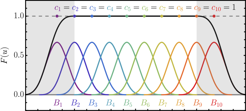
We write the CASE21 exchange and correlation ICFs as linear combinations of $N_{\rm sp}$ compact piece-wise bell-shaped cubic ($k=3$) uniform B-spline basis functions ($\{B_{i}\}$), Eilers and Marx (1996)

$$\begin{split}F_{\rm x}(u_{\rm x,\sigma})&=\sum_{i}^{N_{\rm sp}}c_{{\rm x},i}B_{i}(u_{\rm x,\sigma})=\bm{c}_{\rm x}\cdot\bm{B}_{\rm x,\sigma}\\ F_{\rm c}(u_{\rm c})&=\sum_{i}^{N_{\rm sp}}c_{\rm c,i}B_{i}(u_{\rm c})=\bm{c}_{\rm c}\cdot\bm{B}_{\rm c},\end{split}$$ (6)

which is equivalent to constructing each ICF using a cubic spline Prautzsch et al. (2002) (see Supporting Information (SI) for more details). With the choice of knot vector employed herein, Eilers and Marx (1996); Eilers et al. (2015) the $B_{i}(u_{\rm x,\sigma})$ and $B_{i}(u_{\rm c})$ are uniformly spaced with all points in $0\leq u_{\rm x,\sigma}\leq 1$ and $0\leq u_{\rm c}\leq 1$ supported by three non-zero B-splines. As depicted in Fig. 1(a), setting $\bm{c}_{\rm x}=\bm{1}=\bm{c}_{\rm c}$ in Eq. (6) results in $F_{\rm x}(u_{\rm x,\sigma})=1=F_{\rm c}(u_{\rm c})$; in this limit, CASE21 exchange and correlation reduce to LSDA exchange and LDA correlation, respectively.

Figure 1: (Top) B-spline basis functions ($\{B_{i}\}_{i=1,10}$, rainbow) used to represent the exchange and correlation ICFs in this work. When all expansion coefficients are set to unity, the resulting B-spline curve ($F(u)=\sum_{i}c_{i}B_{i}(u)$, black) is uniform in $0\leq u\leq 1$ and recovers the LSDA/LDA limit. (Bottom) B-spline curve with non-uniform coefficients. Note again how the coefficients closely align with the curve for $0\leq u\leq 1$.

Having defined the CASE21 functional form, we now discuss a general framework that unites NE-DFA and SE-DFA strategies. Namely, we determine $\bm{c}=(\bm{c}_{\rm x},\bm{c}_{\rm c})$ using generalized Tikhonov regularization, Hansen (1998) i.e., by minimizing the following loss function:

$$\mathcal{L}=\left\lVert\bm{X}\bm{c}-\bm{y}\right\rVert_{\bm{W}}^{2}+\lambda\left\lVert\bm{c}\right\rVert_{\bm{A}}^{2}+\eta\sum_{i}\left\lVert\bm{c}-\bm{c}_{0}\right\rVert_{\bm{Q}_{i}}^{2},$$ (7)

where $\left\lVert\bm{v}\right\rVert_{\bm{M}}^{2}=\bm{v}^{\top}\bm{M}\bm{v}$ is the matrix norm of the vector $\bm{v}$ using the matrix $\bm{M}$, the sum is over the enforced constraints, and all other quantities will be defined below. Hence, the key to determining $\bm{c}$ lies in appropriate matrix norm choices in each term in $\mathcal{L}$: goodness of fit, regularization/smoothness, and constraint satisfaction.

Goodness of Fit. In the goodness of fit term, we construct the design matrix $\bm{X}$ by first noting that substitution of Eq. (6) into Eqs. (3)–(4) (with fixed orbitals) casts $E_{\rm x}[\rho_{\sigma}]$ and $E_{\rm c}[\rho,\zeta]$ into linear forms in $\bm{c}_{\rm x}$ and $\bm{c}_{\rm c}$:

$$\begin{split}E_{\rm x}[\rho_{\sigma}]&=\sum_{i}^{N_{\rm sp}}c_{{\rm x},i}\int\rho_{\sigma}\,\epsilon_{\rm x}^{\rm LDA}(\rho_{\sigma})B_{i}(u_{\rm x,\sigma})\,d\bm{r}\equiv\bm{c}_{\rm x}\cdot\bm{\xi}_{{\rm x},\sigma}\\ E_{\rm c}[\rho,\zeta]&=\sum_{i}^{N_{\rm sp}}c_{{\rm c},i}\int\rho\,\epsilon_{\rm c}^{\rm LDA}(\rho,\zeta)B_{i}(u_{\rm c})\,d\bm{r}\equiv\bm{c}_{\rm c}\cdot\bm{\xi}_{{\rm c}}.\end{split}$$ (8)

Linear combinations of $\bm{\xi}_{\rm x,\sigma}$ and $\bm{\xi}_{\rm c}$ can then be used to construct semi-local xc contributions to energy differences $\Delta E_{\rm xc}$ (e.g., atomization energies, reaction energies, barrier heights) in a form amenable to linear regression using reference quantum-mechanical data. Defining $\bm{\xi}\equiv(\bm{\xi}_{\rm x},\bm{\xi}_{\rm c})$, with $\bm{\xi}_{\rm x}$ obtained after applying Eqs. (1)–(2) to $\bm{\xi}_{\rm x,\uparrow}$ and $\bm{\xi}_{\rm x,\downarrow}$ in Eq. (8), allows us to write:

$$\Delta E_{\rm xc} =\sum_{j}\nu_{j}\left(\bm{c}\cdot\bm{\xi}_{j}\right)=\bm{c}\cdot\sum_{j}\nu_{j}\,\bm{\xi}_{j}\equiv\bm{c}\cdot\bm{x},$$ (9)

in which $\nu_{j}$ is the stoichiometric coefficient for the $j$-th component in $\Delta E_{\rm xc}$ (i.e., the energy of a molecule or atom) and $\bm{x}$ is a single row of $\bm{X}$. $\bm{y}$ is the corresponding vector of reference energy differences $\Delta E_{\rm xc}^{\rm ref}$, and our choice for $\bm{W}$ (a square diagonal matrix of weights $w_{i}\equiv 1/\Delta E_{{\rm xc},i}^{\rm ref}$) is motivated by the fact that the $\bm{c}$ minimizing the goodness of fit term only (i.e., weighted least squares) is the best linear unbiased estimator (under some common assumptions) if the $w_{i}$ are inversely proportional to the variance in each measurement. Strutz (2016) Since $E_{\rm xc}$ is the only inexact term in KS-DFT, both bias- and variance-type DFA errors should scale linearly with $E_{\rm xc}$, Ernst et al. ; Kang et al. making this a natural choice for $\bm{W}$. Here, we argue that the piece-wise nature of a B-spline curve offers more flexibility than the low-order polynomial expansions often used to represent SE-DFA ICFs (e.g., the B97 familyMardirossian and Head-Gordon (2017); Becke (1997); Mardirossian and Head-Gordon (2014)); with the ability to conform to more subtle shapes, a B-spline ICF should be able to better leverage the reference data.

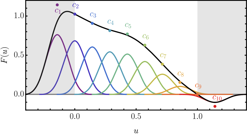
Regularization/Smoothness. For the second term in $\mathcal{L}$, we note that B-splines can be regularized by explicitly penalizing deviations from smoothness (i.e., ICF “wiggles”) using P-splines, a regularization technique suggested by Eilers and Marx Eilers and Marx (1996); Eilers et al. (2015) based on the observation that B-spline coefficients closely resemble the B-spline curve (see Fig. 1(b)). As such, smoothness can be explicitly enforced via a finite-difference penalty on $\bm{c}$; in this work, we interpret non-smoothness as non-linearity in the ICF, and construct $\bm{A}$ from the second-derivative finite-difference matrix (see SI). $\lambda$ is a hyperparameter that governs the relative importance of the regularization/smoothness and goodness of fit contributions to $\mathcal{L}$, and interpolates (assuming $\eta\ggg 1$, vide infra) between linear ICFs (i.e., $\hbox to0.0pt{\hskip 1.40971pt\leavevmode\hbox{\set@color$\overline{\hbox{}}$}\hss}{\leavevmode\hbox{\set@color$F$}}_{\rm x}(u_{\rm x,\sigma})$ and $\hbox to0.0pt{\hskip 1.40971pt\leavevmode\hbox{\set@color$\overline{\hbox{}}$}\hss}{\leavevmode\hbox{\set@color$F$}}_{\rm c}(u_{\rm c})$) that are completely constraint-driven (as $\lambda\rightarrow\infty$) and wiggly ICFs that are data-driven to the maximal amount possible in this framework (as $\lambda\rightarrow 0$). As such, any non-linearity in the final optimized CASE21 ICFs can be attributed to the data. Here, we note that alternative interpretations of smoothness would result in penalizing other derivatives (e.g., $F^{\prime\prime\prime}(u)$). Separately penalizing the exchange and correlation ICFs (i.e., using two $\lambda$-hyperparameters) is also possible if the regularization/smoothness contributions to $\mathcal{L}$ from $F_{\rm x}(u_{\rm x,\sigma})$ and $F_{\rm c}(u_{\rm c})$ strongly differ. In this work, we found that P-spline regularization (which is uniquely enabled by the choice of a B-spline basis) yields ICFs devoid of any spurious “wiggles” via single-$\lambda$ penalization of $F^{\prime\prime}(u)$ (vide infra). In contrast, an excessively large penalty (which results in decreased performance) is usually required to remove all non-physical “bumps” or “wiggles” in polynomial ICFs regularized via Tikhonov (or ridge) regression. Wellendorff et al. (2012); S. Yu et al. (2015) Furthermore, although such polynomial-based smoothness penalties are somewhat effective in reducing DFA grid dependence, Verma and Truhlar (2020); Mardirossian and Head-Gordon (2016) these approaches have been largely ineffective when enforced alongside constraints. Wellendorff et al. (2012); Petzold et al. (2012) On the other hand, we find no issues when simultaneously enforcing ICF smoothness as well as numerous linear and non-linear constraints.

Constraint Satisfaction. During CASE21 construction, we fully enforce the following $10$ constraints: exchange spin scaling, Oliver and Perdew (1979) uniform density scaling for exchange, Levy and Perdew (1985) UEG exchange limit, Kurth et al. (1999) UEG linear response, Perdew et al. (1996) Lieb-Oxford bound, Lieb and Oxford (1981) exchange energy negativity, UEG correlation limit, Kurth et al. (1999) second-order gradient expansion for correlation, Wang and Perdew (1991); Ma and Brueckner (1968); Geldart and Rasolt (1976); Langreth and Perdew (1980) rapidly varying density limit for correlation, Perdew et al. (1996) and correlation energy non-positivity. Perdew et al. (1996) We also partially enforce uniform scaling to the high-density limit for correlation Levy (1989) (vide supra). In the constraint satisfaction term in $\mathcal{L}$, the $\{\bm{Q_{i}}\}$ are chosen to measure constraint-specific deviations of $\bm{c}$ from $\bm{c}_{0}$, the coefficients corresponding to $\hbox to0.0pt{\hskip 1.40971pt\leavevmode\hbox{\set@color$\overline{\hbox{}}$}\hss}{\leavevmode\hbox{\set@color$F$}}_{\rm x}(u_{\rm x,\sigma})$ and $\hbox to0.0pt{\hskip 1.40971pt\leavevmode\hbox{\set@color$\overline{\hbox{}}$}\hss}{\leavevmode\hbox{\set@color$F$}}_{\rm c}(u_{\rm c})$. Each $\bm{Q}_{i}$ corresponds to a constraint on $F(u)$ or $F^{\prime}(u)$, and is constructed such that any constraint-satisfying $\bm{c}$ yields $\left\lVert\bm{c}-\bm{c}_{0}\right\rVert_{\bm{Q}_{i}}^{2}=0$ (see SI for details on $\bm{Q}_{i}$ construction). $\eta$ is a hyperparameter that governs the relative importance of the constraint satisfaction contribution to $\mathcal{L}$, and was chosen to be large enough ($\eta=10^{8}$) for strict constraint satisfaction, but small enough to avoid conditioning issues. Since each B-spline has compact support, each $\bm{Q}_{i}$ only enforces the constraint on a small subset of $\bm{c}$ (e.g., the $\bm{c}$ corresponding to non-zero B-splines at the $u=0$ limit); in contrast, each constraint would generally involve every parameter in a polynomial-based ICF (e.g., MCML Brown et al. (2021)). Another important consequence of this local support is that the B-spline curve will lie within the range of $\bm{c}$ (cf. Fig. 1(b)). Hence, inequality constraints can be enforced via an iterative update to the corresponding $\bm{Q}_{i}$ using the shape constraint algorithm (SCA) of Bollaerts et al., Bollaerts et al. (2006) which fixes all inequality-violating $c_{i}$ to the constraint boundary. In contrast, there is no straightforward way to explicitly apply inequality constraints on a polynomial-based ICF as each basis function is unique and has global support. This highlights another benefit provided by a B-spline basis in the construction of smooth and constraint-satisfying SE-DFAs.

Training Procedure. Our self-consistent training procedure (Scheme 1, see Computational Methods for more details) leverages three distinct data sets (see SI): training ($\bm{X}_{\rm train},\bm{y}_{\rm train}$), validation ($\bm{X}_{\rm val},\bm{y}_{\rm val}$), and testing ($\bm{X}_{\rm test},\bm{y}_{\rm test}$). In a given iteration, the training set (a single database of heavy atom transfer reaction energies, HAT707 Karton et al. (2011); Mardirossian and Head-Gordon (2017)) is used to initially determine $\bm{c}$ by minimizing $\mathcal{L}$ (in conjunction with the SCA for satisfying inequality constraints) for a range of $\lambda$ and a given set of orbitals $\{\psi_{i}\}$ (with initial $\{\psi_{i}^{0}\}$ generated using $\hbox to0.0pt{\hskip 1.40971pt\leavevmode\hbox{\set@color$\overline{\hbox{}}$}\hss}{\leavevmode\hbox{\set@color$F$}}_{\rm x}(u_{\rm x,\sigma})$ and $\hbox to0.0pt{\hskip 1.40971pt\leavevmode\hbox{\set@color$\overline{\hbox{}}$}\hss}{\leavevmode\hbox{\set@color$F$}}_{\rm c}(u_{\rm c})$). With $\bm{c}(\lambda)$, a weighted-root-mean-square error,

$${\rm wRMSE}(\lambda)=\sqrt{{\rm diag}(\bm{W})\cdot\bm{r}(\lambda)^{2}/\operatorname{Tr}{(\bm{W}})},$$ (10)

in which $\bm{r}(\lambda)=\bm{X}_{\rm val}\bm{c}(\lambda)-\bm{y}_{\rm val}$ is the error vector and $\bm{r}(\lambda)^{2}$ is the element-wise square of $\bm{r}(\lambda)$, is computed on the validation set (which contains absolute energies of H–O from AE18 Chakravorty et al. (1993); Mardirossian and Head-Gordon (2017) and all atomization energies in TAE203 Karton et al. (2017); Morgante and Peverati (2019)). Using $\lambda^{*}={\rm argmin}_{\lambda}{\rm wRMSE}(\lambda)$, $\bm{c}^{*}$ is determined by re-optimizing $\mathcal{L}$ (in conjunction with the SCA) over the training and validation sets. New $\{\psi_{i}\}$ are then generated using $\bm{c}^{*}$, and the entire cycle is repeated until $\bm{c}^{*}$ is stationary. At this point, the testing set (which contains a significantly more diverse range of chemical properties than the training and validation sets, vide infra) is used to assess the performance and transferability of the self-consistent DFA.

List of Schemes 1 Self-consistent DFA training procedure.

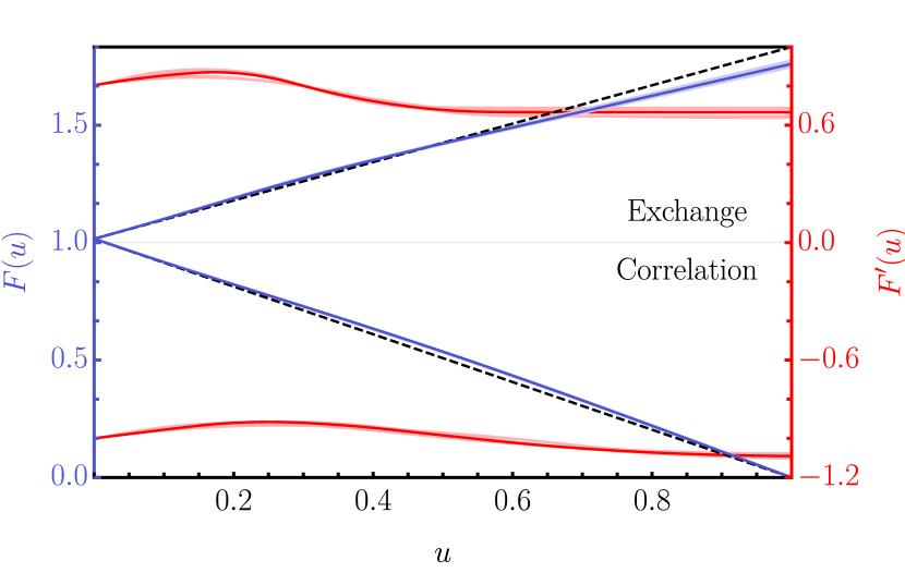
Preliminary fits using $\{\psi_{i}^{0}\}$ suggested that the effective degrees of freedom Ye (1998) (DoF, see SI for derivation) change slowly starting around $N_{\rm sp}=10$, and the performance of the corresponding (non-self-consistently optimized) DFA was representative of those with $N_{\rm sp}>10$. Hence, we used $N_{\rm sp}=10$ in Scheme 1 to generate the self-consistently optimized CASE21 DFA (six iterations; convergence criterion: $|\Delta\bm{c}|<10^{-5}$; see SI for $\bm{c}^{*}$). Even with a finite $\eta$, CASE21 nearly exactly satisfies all enforced constraints, i.e., $F_{\rm x}(0)$, $F_{\rm c}(0)$, $F_{\rm x}^{\prime}(0)$, and $F_{\rm c}^{\prime}(0)$ differ from their corresponding exact values by ${\sim}10^{-5}$, $F_{\rm c}(1)$ differs by ${\sim}10^{-6}$, and all other constraints are exactly satisfied. We therefore conclude that the proposed CASE framework (i.e., Tikhonov regularization in conjunction with P-splines) successfully enforced all constraints without sacrificing smoothness, which still remains a challenge for other DFA training procedures. Wellendorff et al. (2012); Petzold et al. (2012) To confirm that CASE21 remains representative of DFAs trained with other $N_{\rm sp}$ values, we (non-self-consistently) optimized $\bm{c}$ for select $N_{\rm sp}\in[6,40]$ using the CASE21 $\{\psi_{i}\}$. As depicted in Fig. 2, the resulting ICFs and their first derivatives were all smooth and very similar (particularly for $N_{\rm sp}\geq 10$), thereby providing an a posteriori justification for our choice of $N_{\rm sp}=10$ for CASE21. From this plot, one can also see that the CASE21 ICFs (${\rm DoF}=1.22$) subtly deviate from linearity in ways that simply cannot be obtained using low-order polynomial expansions.

Figure 2: (Top) Exchange and correlation ICFs (blue) and first derivatives (red) for select $N_{\rm sp}\in[6,40]$. Highlighted curves (dark blue and dark red) correspond to the self-consistently optimized CASE21 DFA (with $N_{\rm sp}=10$). Dashed lines represent the parameter-free linear ICFs ($\hbox to0.0pt{\hskip 1.40971pt\leavevmode\hbox{\set@color$\overline{\hbox{}}$}\hss}{\leavevmode\hbox{\set@color$F$}}_{\rm x}(u_{\rm x,\sigma})$ and $\hbox to0.0pt{\hskip 1.40971pt\leavevmode\hbox{\set@color$\overline{\hbox{}}$}\hss}{\leavevmode\hbox{\set@color$F$}}_{\rm c}(u_{\rm c})$) designed to satisfy the same constraints as CASE21. (Bottom) Effective degrees of freedom (DoF) for select $N_{\rm sp}\in[6,40]$, with the dark purple point corresponding to CASE21.

Figure 3: Mean absolute errors of CASE21 (blue), PBE0 (gray), and B3LYP (orange) in the training/validation (shaded region) and testing (white region) sets. Bar labels indicate the relative performance of CASE21 and PBE0 (green: ${\rm MAE}^{\rm CASE21}<{\rm MAE}^{\rm PBE0}$; red: ${\rm MAE}^{\rm CASE21}>{\rm MAE}^{\rm PBE0}$). Properties (number of data points) include: HAT—heavy atom transfer reaction energies, Karton et al. (2011); Mardirossian and Head-Gordon (2017) TAE—total atomization energies, Karton et al. (2017); Morgante and Peverati (2019) AE—absolute energies, Chakravorty et al. (1993); Mardirossian and Head-Gordon (2017) RXN—reaction energies, Goerigk and Grimme (2010); Zhao et al. (2005, 2004); Mardirossian and Head-Gordon (2017); Goerigk et al. (2017); Curtiss et al. (1997); Morgante and Peverati (2019); Neese et al. (2009); Karton et al. (2011, 2012) BDE—bond dissociation energies, Yu and Truhlar (2015); Karton et al. (2011); Mardirossian and Head-Gordon (2017); Goerigk et al. (2017); Morgante and Peverati (2019) PA—proton affinities, Goerigk et al. (2017); Parthiban and Martin (2001); Zhao and Truhlar (2006); Morgante and Peverati (2019) BH—barrier heights, Zhao et al. (2004, 2005); Mardirossian and Head-Gordon (2017); Goerigk et al. (2017); Morgante and Peverati (2019) IP—ionization potentials, Curtiss et al. (1991); Lynch et al. (2003); Goerigk and Grimme (2010); Goerigk et al. (2017); Morgante and Peverati (2019); Mardirossian and Head-Gordon (2017) EA—electron affinities, Lynch et al. (2003); Curtiss et al. (1991); Goerigk and Grimme (2010); Mardirossian and Head-Gordon (2017) IE—isomerization energies, Gruzman et al. (2009); Wilke et al. (2009); Yu et al. (2015); Lao and Herbert (2015); Grimme et al. (2007); Peverati and Truhlar (2014); Luo et al. (2011); Martin (2013); Zhao and Truhlar (2006); Zhao et al. (2005); Zhao and Truhlar (2006); Csonka et al. (2009); Mardirossian et al. (2013); Kesharwani et al. (2016); Karton et al. (2011); Mardirossian and Head-Gordon (2017); Goerigk et al. (2017); Goerigk and Grimme (2010); Morgante and Peverati (2019) and NCI—non-covalent interaction energies. Řezáč and Hobza (2013, 2012); Boese (2013, 2015, 2015); Smith et al. (2014); Kozuch and Martin (2013); Mardirossian and Head-Gordon (2017)

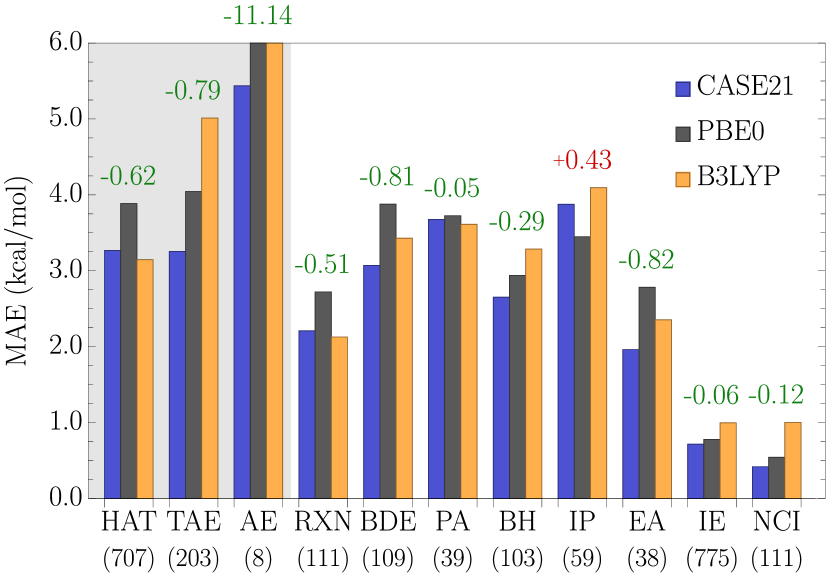
Final Testing. The performance of CASE21 across a diverse set of chemical properties is compared to that of the PBE0 and B3LYP hybrid DFAs in Fig. 3. CASE21 outperforms the PBE0 NE-DFA on $10/11$ properties, with improvements as large as $0.81$ kcal/mol and $0.82$ kcal/mol for bond dissociation energies and electron affinities, respectively. In the testing set, CASE21 improves upon PBE0 in $7/8$ properties by an average of $0.38$ kcal/mol. On the other hand, PBE0 only outperforms CASE21 for ionization potentials. CASE21 also outperforms B3LYP (a popular SE-DFA for chemical applications) on $8/11$ properties; in the testing set, CASE21 improves upon B3LYP in $6/8$ properties by an average of $0.41$ kcal/mol (while B3LYP only offers a marginal ${\sim}0.07$ kcal/mol improvement on the remaining $2/8$). We therefore conclude that CASE21 preserves the physical rigor and transferability of the PBE0 NE-DFA while still outperforming the B3LYP SE-DFA. Although the CASE21 ICFs are clearly smooth (cf. Fig. 2), we also investigated the grid dependence of this DFA for completeness. Since Lebedev-Treutler grids Treutler and Ahlrichs (1995) with $50$ radial and $194$ angular grid points (i.e., $(50,194)$) are typically large enough to obtain accurate energetics with standard hybrid GGAs (such as PBE0), Dasgupta and Herbert (2017) we compared the performance of CASE21 using this grid to the larger grids employed during the training procedure (see Computational Methods). Using all points in the training, validation, and testing data sets ($N=2{,}263$), we find nearly identical mean absolute deviations of $1.84\times 10^{-2}$ kcal/mol for CASE21 and $1.83\times 10^{-2}$ kcal/mol for PBE0, thereby indicating that CASE21 does not require larger quadrature grids than PBE0 for accurate integration.

In this work, we presented the CASE (Constrained And Smoothed semi-Empirical) framework for uniting NE-DFA and SE-DFA construction paradigms. By employing a B-spline representation for the ICFs, this approach has several distinct advantages over the historical choice of a polynomial basis, namely, explicit enforcement of linear and non-linear constraints (using Tikhonov regularization) as well as explicit penalization of non-physical ICF “bumps” or “wiggles” (using P-splines). As proof of concept, we used this approach to construct CASE21, a hybrid GGA that completely satisfies all but one constraint (and partially satisfies the remaining one) met by the PBE0 NE-DFA. Despite being trained on only a handful of properties, CASE21 outperforms PBE0 and B3LYP (arguably the most popular SE-DFA for chemical applications) across a diverse set of chemical properties. As such, we argue that the CASE framework can be used to design next-generation DFAs that maintain the physical rigor and transferability of NE-DFAs while leveraging benchmark quantum-mechanical data to remove the arbitrariness of ansatz selection and improve performance. Future work will extend this approach to more sophisticated DFAs (e.g., meta-GGAs, range-separated hybrids) as well as explore the use of B-splines in constructing robust features for machine-learning chemical properties.

Computational Methods

All electronic structure calculations were performed using in-house versions of Psi4 (v1.3.2) Parrish et al. (2017) and LibXC (v4.3.4) Lehtola et al. (2018) modified with a self-consistent implementation of the CASE21 DFA (including functional derivatives analytically computed using Mathematica v12.1). All self-consistent field (SCF) calculations were performed using density fitting (DF) in conjunction with the def2-QZVPPD Weigend et al. (2003); Rappoport and Furche (2010) and def2-QZVPP-JKFIT Schuchardt et al. (2007) basis sets and an energy convergence threshold of e_convergence = 1e-12. During DFA training, all calculations employed $(99,590)$ Lebedev-Treutler grids Treutler and Ahlrichs (1995) except for the calculations of the absolute energies in AE18, Chakravorty et al. (1993); Mardirossian and Head-Gordon (2017) which used $(500,974)$. Minimization of $\mathcal{L}$ in Eq. (7) and optimization of ${\rm wRMSE}(\lambda)$ in Eq. (10) were performed in Mathematica v12.1.

Supporting Information Available:

Supporting Information (SI) includes:

B-spline definitions; Enforcement of ICF constraints; Training, validation, and testing data sets; Derivation of optimal coefficients and effective degrees of freedom for weighted generalized Tikhonov regularization; Optimized CASE21 ICF coefficients.

TOC Graphic

References

- Mardirossian and Head-Gordon (2017) Mardirossian, N.; Head-Gordon, M. Thirty years of density functional theory in computational chemistry: An overview and extensive assessment of 200 density functionals. Mol. Phys. 2017, 115, 2315–2372.
- Perdew and Schmidt (2001) Perdew, J. P.; Schmidt, K. Jacob’s ladder of density functional approximations for the exchange-correlation energy. AIP Conf. Proc. 2001, 577, 1–20.
- Becke (1997) Becke, A. D. Density-functional thermochemistry. V. Systematic optimization of exchange-correlation functionals. J. Chem. Phys. 1997, 107, 8554–8560.
- Perdew et al. (1996) Perdew, J. P.; Burke, K.; Ernzerhof, M. Generalized gradient approximation made simple. Phys. Rev. Lett. 1996, 77, 3865–3868.
- Kurth et al. (1999) Kurth, S.; Perdew, J. P.; Blaha, P. Molecular and solid-state tests of density functional approximations: LSD, GGAs, and meta-GGAs. Int. J. Quantum Chem. 1999, 75, 889–909.
- Wang and Perdew (1991) Wang, Y.; Perdew, J. P. Spin scaling of the electron-gas correlation energy in the high-density limit. Phys. Rev. B 1991, 43, 8911–8916.
- Ma and Brueckner (1968) Ma, S.-K.; Brueckner, K. A. Correlation energy of an electron gas with a slowly varying high density. Phys. Rev. 1968, 165, 18–31.
- Geldart and Rasolt (1976) Geldart, D. J. W.; Rasolt, M. Exchange and correlation energy of an inhomogeneous electron gas at metallic densities. Phys. Rev. B 1976, 13, 1477–1488.
- Langreth and Perdew (1980) Langreth, D. C.; Perdew, J. P. Theory of nonuniform electronic systems. I. Analysis of the gradient approximation and a generalization that works. Phys. Rev. B 1980, 21, 5469–5493.
- Adamo and Barone (1999) Adamo, C.; Barone, V. Toward reliable density functional methods without adjustable parameters: The PBE0 model. J. Chem. Phys. 1999, 110, 6158–6170.
- Sun et al. (2015) Sun, J.; Ruzsinszky, A.; Perdew, J. P. Strongly constrained and appropriately normed semilocal density functional. Phys. Rev. Lett. 2015, 115, 036402.
- Becke (1993) Becke, A. D. Density-functional thermochemistry. III. The role of exact exchange. J. Chem. Phys. 1993, 98, 5648–5652.
- Peverati and Truhlar (2014) Peverati, R.; Truhlar, D. G. Quest for a universal density functional: The accuracy of density functionals across a broad spectrum of databases in chemistry and physics. Philos. Trans. R. Soc. A 2014, 372, 20120476.
- Zhao et al. (2005) Zhao, Y.; Schultz, N. E.; Truhlar, D. G. Exchange-correlation functional with broad accuracy for metallic and nonmetallic compounds, kinetics, and noncovalent interactions. J. Chem. Phys. 2005, 123, 161103.
- Zhao and Truhlar (2008) Zhao, Y.; Truhlar, D. G. The M06 suite of density functionals for main group thermochemistry, thermochemical kinetics, noncovalent interactions, excited states, and transition elements: Two new functionals and systematic testing of four M06-class functionals and 12 other functionals. Theor. Chem. Acc. 2008, 120, 215–241.
- Mardirossian and Head-Gordon (2014) Mardirossian, N.; Head-Gordon, M. B97X-V: A 10-parameter, range-separated hybrid, generalized gradient approximation density functional with nonlocal correlation, designed by a survival-of-the-fittest strategy. Phys. Chem. Chem. Phys. 2014, 16, 9904–9924.
- Perdew et al. (2005) Perdew, J. P.; Ruzsinszky, A.; Tao, J.; Staroverov, V. N.; Scuseria, G. E.; Csonka, G. I. Prescription for the design and selection of density functional approximations: More constraint satisfaction with fewer fits. J. Chem. Phys. 2005, 123, 62201.
- Yu et al. (2016) Yu, H. S.; Li, S. L.; Truhlar, D. G. Perspective: Kohn-Sham density functional theory descending a staircase. J. Chem. Phys. 2016, 145, 130901.
- Medvedev et al. (2017) Medvedev, M. G.; Bushmarinov, I. S.; Sun, J.; Perdew, J. P.; Lyssenko, K. A. Density functional theory is straying from the path toward the exact functional. Science 2017, 355, 49–52.
- Dasgupta and Herbert (2017) Dasgupta, S.; Herbert, J. M. Standard grids for high-precision integration of modern density functionals: SG-2 and SG-3. J. Comput. Chem. 2017, 38, 869–882.
- Mardirossian and Head-Gordon (2016) Mardirossian, N.; Head-Gordon, M. How accurate are the Minnesota density functionals for noncovalent interactions, isomerization energies, thermochemistry, and barrier heights involving molecules composed of main-group elements? J. Chem. Theory Comput. 2016, 12, 4303–4325.
- Wheeler and Houk (2011) Wheeler, S. E.; Houk, K. N. Integration grid errors for meta-GGA-predicted reaction energies: Origin of grid errors for the M06 suite of functionals. J. Chem. Theory Comput. 2011, 6, 395–404.
- Bootsma and Wheeler (2019) Bootsma, A. N.; Wheeler, S. E. Popular integration grids can result in large errors in DFT-computed free energies. ChemRxiv 2019, This content is a preprint and has not been peer-reviewed.
- Brown et al. (2021) Brown, K.; Maimaiti, Y.; Trepte, K.; Bligaard, T.; Voss, J. MCML: Combining physical constraints with experimental data for multi-purpose meta-generalized gradient approximation. J. Comput. Chem. 2021, 42, 2004–2013.
- Wellendorff et al. (2012) Wellendorff, J.; Lundgaard, K. T.; Møgelhøj, A.; Petzold, V.; Landis, D. D.; Nørskov, J. K.; Bligaard, T.; Jacobsen, K. W. Density functionals for surface science: Exchange-correlation model development with Bayesian error estimation. Phys. Rev. B 2012, 85, 235149.
- Wellendorff et al. (2014) Wellendorff, J.; Lundgaard, K. T.; Jacobsen, K. W.; Bligaard, T. mBEEF: An accurate semi-local Bayesian error estimation density functional. J. Chem. Phys. 2014, 140, 144107.
- Lundgaard et al. (2016) Lundgaard, K. T.; Wellendorff, J.; Voss, J.; Jacobsen, K. W.; Bligaard, T. mBEEF-vdW: Robust fitting of error estimation density functionals. Phys. Rev. B 2016, 93, 235162.
- Verma and Truhlar (2020) Verma, P.; Truhlar, D. G. Status and challenges of density functional theory. Trends Chem. 2020, 2, 302–318.
- Zhao et al. (2006) Zhao, Y.; Schultz, N. E.; Truhlar, D. G. Design of density functionals by combining the method of constraint satisfaction with parametrization for thermochemistry, thermochemical kinetics, and noncovalent interactions. J. Chem. Theory Comput. 2006, 2, 364–382.
- Eilers and Marx (1996) Eilers, P. H. C.; Marx, B. D. Flexible smoothing with B-splines and penalties. Stat. Sci. 1996, 11, 89–121.
- Eilers et al. (2015) Eilers, P. H. C.; Marx, B. D.; Durbán, M. Twenty years of P-splines. SORT 2015, 39, 149–186.
- Ernzerhof and Scuseria (1999) Ernzerhof, M.; Scuseria, G. E. Assessment of the Perdew–Burke–Ernzerhof exchange-correlation functional. J. Chem. Phys. 1999, 110, 5029–5036.
- Oliver and Perdew (1979) Oliver, G. L.; Perdew, J. P. Spin-Density Gradient Expansion for the Kinetic Energy. Phys. Rev. A 1979, 20, 397–403.
- Becke (1986) Becke, A. D. Density functional calculations of molecular bond energies. J. Chem. Phys. 1986, 84, 4524–4529.
- Lieb and Oxford (1981) Lieb, E. H.; Oxford, S. Improved lower bound on the indirect coulomb energy. Int. J. Quantum Chem. 1981, 19, 427–439.
- Perdew and Wang (1992) Perdew, J. P.; Wang, Y. Accurate and simple analytic representation of the electron-gas correlation energy. Phys. Rev. B 1992, 45, 13244–13249.
- Levy (1989) Levy, M. Asymptotic coordinate scaling bound for exchange-correlation energy in density-functional theory. Int. J. Quantum Chem. 1989, 36, 617–619.
- (38) Although the CASE21 correlation form is able to exactly cancel the LDA logarithmic singularity, the correlation energy completely vanishes in this limit. However, to fully satisfy uniform scaling to the high-density limit for correlation, the correlation energy should be non-zero in this limit, e.g., Hartree for a two-electron atom as . Perdew et al. (1996)
- Prautzsch et al. (2002) Prautzsch, H.; Boehm, W.; Paluszny, M. Bezier and B-Spline Techniques, 1st ed.; Springer-Verlag, Berlin, Germany, 2002.
- Hansen (1998) Hansen, P. C. Rank-Deficient and Discrete Ill-Posed Problems; Mathematical Modeling and Computation; SIAM, Philadelphia, Pennsylvania, 1998.
- Strutz (2016) Strutz, T. Data Fitting and Uncertainty: A Practical Introduction to Weighted Least Squares and Beyond, 2nd ed.; Springer Vieweg, Wiesbaden, Germany, 2016.
- (42) Ernst, B. G.; Sparrow, Z. M.; DiStasio Jr., R. A. NENCI-2021 part II: Evaluating the performance of quantum chemical approximations on the NENCI-2021 benchmark database. (in preparation).
- (43) Kang, R.; Sparrow, Z. M.; Ernst, B. G.; DiStasio Jr., R. A. NECI-2021: A large benchmark database of non-equilibrium covalent interactions. (in preparation).
- S. Yu et al. (2015) S. Yu, H.; Zhang, W.; Verma, P.; He, X.; G. Truhlar, D. Nonseparable exchange–correlation functional for molecules, including homogeneous catalysis involving transition metals. Phys. Chem. Chem. Phys. 2015, 17, 12146–12160.
- Petzold et al. (2012) Petzold, V.; Bligaard, T.; Jacobsen, K. W. Construction of new electronic density functionals with error estimation through fitting. Top. Catal. 2012, 55, 402–417.
- Levy and Perdew (1985) Levy, M.; Perdew, J. P. Hellmann-Feynman, virial, and scaling requisites for the exact universal density functionals. Shape of the correlation potential and diamagnetic susceptibility for atoms. Phys. Rev. A 1985, 32, 2010–2021.
- Bollaerts et al. (2006) Bollaerts, K.; Eilers, P. H. C.; van Mechelen, I. Simple and multiple P-splines regression with shape constraints. Br. J. Math. Stat. Psychol. 2006, 59, 451–469.
- Karton et al. (2011) Karton, A.; Daon, S.; Martin, J. M. L. W4-11: A high-confidence benchmark dataset for computational thermochemistry derived from first-principles W4 data. Chem. Phys. Lett. 2011, 510, 165–178.
- Chakravorty et al. (1993) Chakravorty, S. J.; Gwaltney, S. R.; Davidson, E. R.; Parpia, F. A.; Fischer, C. F. Ground-state correlation energies for atomic ions with 3 to 18 electrons. Phys. Rev. A 1993, 47, 3649–3670.
- Karton et al. (2017) Karton, A.; Sylvetsky, N.; Martin, J. M. L. W4-17: A diverse and high-confidence dataset of atomization energies for benchmarking high-level electronic structure methods. J. Comput. Chem. 2017, 38, 2063–2075.
- Morgante and Peverati (2019) Morgante, P.; Peverati, R. ACCDB: A collection of chemistry databases for broad computational purposes. J. Comput. Chem. 2019, 40, 839–848.
- Ye (1998) Ye, J. On measuring and correcting the effects of data mining and model selection. J. Am. Stat. Assoc. 1998, 93, 120–131.
- Goerigk and Grimme (2010) Goerigk, L.; Grimme, S. A general database for main group thermochemistry, kinetics, and noncovalent interactions—assessment of common and reparameterized (meta-)GGA density functionals. J. Chem. Theory Comput. 2010, 6, 107–126.
- Zhao et al. (2005) Zhao, Y.; González-García, N.; Truhlar, D. G. Benchmark database of barrier heights for heavy atom transfer, nucleophilic substitution, association, and unimolecular reactions and its use to test theoretical methods. J. Phys. Chem. A 2005, 109, 2012–2018.
- Zhao et al. (2004) Zhao, Y.; Lynch, B. J.; Truhlar, D. G. Development and assessment of a new hybrid density functional model for thermochemical kinetics. J. Phys. Chem. A 2004, 108, 2715–2719.
- Goerigk et al. (2017) Goerigk, L.; Hansen, A.; Bauer, C.; Ehrlich, S.; Najibi, A.; Grimme, S. A look at the density functional theory zoo with the advanced GMTKN55 database for general main group thermochemistry, kinetics and noncovalent interactions. Phys. Chem. Chem. Phys. 2017, 19, 32184–32215.
- Curtiss et al. (1997) Curtiss, L. A.; Raghavachari, K.; Redfern, P. C.; Pople, J. A. Assessment of Gaussian-2 and density functional theories for the computation of enthalpies of formation. J. Chem. Phys. 1997, 106, 1063–1079.
- Neese et al. (2009) Neese, F.; Schwabe, T.; Kossmann, S.; Schirmer, B.; Grimme, S. Assessment of orbital-optimized, spin-component scaled second-order many-body perturbation theory for thermochemistry and kinetics. J. Chem. Theory Comput. 2009, 5, 3060–3073.
- Karton et al. (2012) Karton, A.; O’Reilly, R. J.; Radom, L. Assessment of theoretical procedures for calculating barrier heights for a diverse set of water-catalyzed proton-transfer reactions. J. Phys. Chem. A 2012, 116, 4211–4221.
- Yu and Truhlar (2015) Yu, H.; Truhlar, D. G. Components of the bond energy in polar diatomic molecules, radicals, and ions formed by group-1 and group-2 metal atoms. J. Chem. Theory Comput. 2015, 11, 2968–2983.
- Parthiban and Martin (2001) Parthiban, S.; Martin, J. M. L. Assessment of W1 and W2 theories for the computation of electron affinities, ionization potentials, heats of formation, and proton affinities. J. Chem. Phys. 2001, 114, 6014–6029.
- Zhao and Truhlar (2006) Zhao, Y.; Truhlar, D. G. Assessment of density functionals for Systems: Energy differences between cumulenes and poly-ynes; proton affinities, bond length alternation, and torsional potentials of conjugated polyenes; and proton affinities of conjugated shiff bases. J. Phys. Chem. A 2006, 110, 10478–10486.
- Curtiss et al. (1991) Curtiss, L. A.; Raghavachari, K.; Trucks, G. W.; Pople, J. A. Gaussian-2 theory for molecular energies of first- and second-row compounds. J. Chem. Phys. 1991, 94, 7221–7230.
- Lynch et al. (2003) Lynch, B. J.; Zhao, Y.; Truhlar, D. G. Effectiveness of diffuse basis functions for calculating relative energies by density functional theory. J. Phys. Chem. A 2003, 107, 1384–1388.
- Gruzman et al. (2009) Gruzman, D.; Karton, A.; Martin, J. M. L. Performance of ab initio and density functional methods for conformational equilibria of CnH2n+2 alkane isomers (n = 4-8). J. Phys. Chem. A 2009, 113, 11974–11983.
- Wilke et al. (2009) Wilke, J. J.; Lind, M. C.; Schaefer III, H. F.; Császár, A. G.; Allen, W. D. Conformers of gaseous cysteine. J. Chem. Theory Comput. 2009, 5, 1511–1523.
- Yu et al. (2015) Yu, L.-J.; Sarrami, F.; Karton, A.; O’Reilly, R. J. An assessment of theoretical procedures for -conjugation stabilisation energies in enones. Mol. Phys. 2015, 113, 1284–1296.
- Lao and Herbert (2015) Lao, K. U.; Herbert, J. M. Accurate and efficient quantum chemistry calculations for noncovalent interactions in many-body systems: the XSAPT family of methods. J. Phys. Chem. A 2015, 119, 235–252.
- Grimme et al. (2007) Grimme, S.; Steinmetz, M.; Korth, M. How to compute isomerization energies of organic molecules with quantum chemical methods. J. Org. Chem. 2007, 72, 2118–2126.
- Luo et al. (2011) Luo, S.; Zhao, Y.; Truhlar, D. G. Validation of electronic structure methods for isomerization reactions of large organic molecules. Phys. Chem. Chem. Phys. 2011, 13, 13683–13689.
- Martin (2013) Martin, J. M. L. What can we learn about dispersion from the conformer surface of n-pentane? J. Phys. Chem. A 2013, 117, 3118–3132.
- Zhao and Truhlar (2006) Zhao, Y.; Truhlar, D. G. A new local density functional for main-group thermochemistry, transition metal bonding, thermochemical kinetics, and noncovalent interactions. J. Chem. Phys. 2006, 125, 194101.
- Csonka et al. (2009) Csonka, G. I.; French, A. D.; Johnson, G. P.; Stortz, C. A. Evaluation of density functionals and basis sets for carbohydrates. J. Chem. Theory Comput. 2009, 5, 679–692.
- Mardirossian et al. (2013) Mardirossian, N.; Lambrecht, D. S.; McCaslin, L.; Xantheas, S. S.; Head-Gordon, M. The performance of density functionals for sulfate–water clusters. J. Chem. Theory Comput. 2013, 9, 1368–1380.
- Kesharwani et al. (2016) Kesharwani, M. K.; Karton, A.; Martin, J. M. L. Benchmark ab initio conformational energies for the proteinogenic amino acids through explicitly correlated methods. Assessment of density functional methods. J. Chem. Theory Comput. 2016, 12, 444–454.
- Řezáč and Hobza (2013) Řezáč, J.; Hobza, P. Describing noncovalent interactions beyond the common approximations: How accurate is the “gold standard,” CCSD(T) at the complete basis set limit? J. Chem. Theory Comput. 2013, 9, 2151–2155.
- Řezáč and Hobza (2012) Řezáč, J.; Hobza, P. Advanced corrections of hydrogen bonding and dispersion for semiempirical quantum mechanical methods. J. Chem. Theory Comput. 2012, 8, 141–151.
- Boese (2013) Boese, A. D. Assessment of coupled cluster theory and more approximate methods for hydrogen bonded systems. J. Chem. Theory Comput. 2013, 9, 4403–4413.
- Boese (2015) Boese, A. D. Basis set limit coupled-cluster studies of hydrogen-bonded systems. Mol. Phys. 2015, 113, 1618–1629.
- Boese (2015) Boese, A. D. Density functional theory and hydrogen bonds: Are we there yet? ChemPhysChem 2015, 16, 978–985.
- Smith et al. (2014) Smith, D. G. A.; Jankowski, P.; Slawik, M.; Witek, H. A.; Patkowski, K. Basis set convergence of the post-CCSD(T) contribution to noncovalent interaction energies. J. Chem. Theory Comput. 2014, 10, 3140–3150.
- Kozuch and Martin (2013) Kozuch, S.; Martin, J. M. L. Halogen bonds: Benchmarks and theoretical analysis. J. Chem. Theory Comput. 2013, 9, 1918–1931.
- Treutler and Ahlrichs (1995) Treutler, O.; Ahlrichs, R. Efficient molecular numerical integration schemes. J. Chem. Phys. 1995, 102, 346–354.
- Parrish et al. (2017) Parrish, R. M.; Burns, L. A.; Smith, D. G. A.; Simmonett, A. C.; DePrince, A. E.; Hohenstein, E. G.; Bozkaya, U.; Sokolov, A. Y.; Di Remigio, R.; Richard, R. M.; Gonthier, J. F.; James, A. M.; McAlexander, H. R.; Kumar, A.; Saitow, M.; Wang, X.; Pritchard, B. P.; Verma, P.; Schaefer III, H. F.; Patkowski, K.; King, R. A.; Valeev, E. F.; Evangelista, F. A.; Turney, J. M.; Crawford, T. D.; Sherrill, C. D. Psi4 1.1: An open-source electronic structure program emphasizing automation, advanced libraries, and interoperability. J. Chem. Theory Comput. 2017, 13, 3185–3197.
- Lehtola et al. (2018) Lehtola, S.; Steigemann, C.; Oliveira, M. J. T.; Marques, M. A. L. Recent developments in libxc—A comprehensive library of functionals for density functional theory. SoftwareX 2018, 7, 1–5.
- Weigend et al. (2003) Weigend, F.; Furche, F.; Ahlrichs, R. Gaussian basis sets of quadruple zeta valence quality for atoms H-Kr. J. Chem. Phys. 2003, 119, 12753–12762.
- Rappoport and Furche (2010) Rappoport, D.; Furche, F. Property-optimized Gaussian basis sets for molecular response calculations. J. Chem. Phys. 2010, 133, 134105.
- Schuchardt et al. (2007) Schuchardt, K. L.; Didier, B. T.; Elsethagen, T.; Sun, L.; Gurumoorthi, V.; Chase, J.; Li, J.; Windus, T. L. Basis set exchange: A community database for computational sciences. J. Chem. Inf. Model. 2007, 47, 1045–1052.