System Identification in Multi-Actuator Hard Disk Drives with Colored Noises using Observer/Kalman Filter Identification (OKID) Framework

Abstract

Multi Actuator Technology in Hard Disk Drives (HDDs) equips drives with two dual stage actuators (DSA) each comprising of a voice coil motor (VCM) actuator and a piezoelectric micro actuator (MA) operating on the same pivot point. Each DSA is responsible for controlling half of the drive’s arms. As both the DSAs operate independently on the same pivot timber, the control forces and torques generated by one affect the operation of the other. The feedback controllers might not completely reject these transferred disturbances and a need to design feedforward controllers arises, which require a good model of the disturbance process. The usual system identification techniques produce a biased estimate because of the presence of the runout which is a colored noise. In this paper, we use the OKID framework to estimate this disturbance cross transfer function from the VCM control input of one DSA to the output of the other DSA from the collected time series data corrupted by colored noise.

I Introduction

In 2017, Seagate unveiled its new multi actuator technology as a breakthrough that can double the data transfer performance of the future-generation hard drives for hyper-scale data centers. In a multi actuator drive, the read-write (R/W) heads are split into two sets, an upper and a lower half, which can double the data transfer rate by having the upper and lower platter sets work in parallel.

The multi actuator setup brought some new challenges to the HDD’s controller design. Since both the DSAs operate on the same pivot point, the forces and torques generated by one DSA can affect the operation of the other DSA. The interaction of the two DSAs can be categorized into three basic scenarios. In the first scenario, both DSAs are in track following mode, and it is expected that the interaction between the two actuators is negligible. In the second scenario, both the DSAs are in seek mode. In this mode, the coupling vibrational interaction is usually negligible compared to the large trajectories for both DSAs. In the third scenario, one DSA is in seek mode and the other is in track following mode. Under this scenario, the seeking DSA will impart disturbances in the form of vibration to the track following DSA, which hamper the performance of the track following DSA drastically. The feedback controllers might not completely reject these transferred disturbances and a need to design feedforward controllers arises, which require a good model of the disturbance process.

Modern HDDs use the inbuilt actuators to write the servo tracks instead of a servowriter or disk writer to reduce the cost of manufacturing. A servowriter uses big motors and robust equipment to write the servo tracks precisely which would be too bulky to be incorporated in a HDD. This amount of precision is not possible during the writing process by a HDD itself as the actuators are not as robust as a servowriter. The disturbances such as spindle vibrations, windage etc affect the writing process and hence the servo tracks are not exactly circles as desired. This offset is called the runout which can be modeled as white noise colored by some stable disturbance process. The presence of this runout corrupts the time series signals by a colored noise.

System identification techniques like the series-parallel algorithm produce a biased estimate even when the signal is corrupted by white noise. Parallel predictors though estimate an unbiased estimate, they suffer from stability issues and coming up with the necessary filters requires apriori knowledge of the system. In this paper, we modify the Observer/Kalman filter Identification (OKID) technique to estimate this disturbance cross transfer function from the VCM control input of one DSA to the output of the other DSA by using the collected time series data corrupted by colored noise.

OKID [1, 3, 5, 6, 7] is a method of identification of a linear dynamical system along with the associated Kalman filter from input-output measurements corrupted by noise. OKID was originally developed at NASA as the OKID/ERA algorithm. Compared to other approaches, OKID is formulated via state observers providing an intuitive interpretation from a control theory perspective.

II Observer/Kalman filter Identification formulation

In this section, we modify the OKID algorithm to account for colored noises. We formulate for the case when a colored noise is added to the output of the system as the runout in HDDs is colored, but the same technique can be used when the process noise is also colored. Consider the following dynamical system of interest

$$\ \begin{split}x_{a}(k+1)=A_{a}x(k)+B_{a}u(k)+\bar{w}_{p}(k)\\ y_{a}(k)=C_{a}x_{a}(k)+D_{a}u(k)+w_{cm}(k)\end{split}$$ (1)

where $x_{a}(k)$ is the state of the system, $\bar{w}_{p}(k)$ is a white process noise, $u(k)$ is the known control input, $y_{a}(k)$ is the measured output, $w_{cm}$ is a colored noise (runout in the case of a HDD) and ($A_{a},B_{a},C_{a},D_{a}$) represent the state, control, output and feedthrough matrices respectively of the actual system. The subscript ’a’ is used for the actual system of interest.

The colored noise can be assumed to be the output of a stable dynamical system with a white noise as its input as follows

$$\begin{split}x_{c}(k+1)=A_{c}x(k)+w_{wm}(k)\\ y_{c}(k)=C_{c}x_{c}(k)+D_{c}w_{wm}(k)\end{split}$$ (2)

where $x_{c}(k)$ is the state of the coloring process, $w_{wm}(k)$ is a white noise, $y_{c}(k)$ is is the colored noise ($y_{c}(k)=w_{cm}(k)$) and ($A_{c},B_{c},C_{c},D_{c}$) represent the state, control, output and feedthrough matrices respectively of the coloring process. The subscript ’c’ is used for the coloring process.

Both the dynamical systems in (1) and (2) can be augmented to form

$$\begin{split}x(k+1)&=Ax(k)+Bu(k)+w_{p}(k)\\ y(k)&=Cx(k)+Du(k)+w_{m}(k)\end{split}$$ (3)

where

$$x=\begin{bmatrix}x_{a}\\ x_{c}\end{bmatrix},A=\begin{bmatrix}A_{a}&0\\ 0&A_{c}\end{bmatrix},B=\begin{bmatrix}B_{a}\\ 0\end{bmatrix},C=\begin{bmatrix}C_{a}&C_{c}\end{bmatrix},\\ D=D_{a},w_{p}=\begin{bmatrix}\bar{w}_{p}\\ w_{m}\end{bmatrix}\;\&\;w_{m}=D_{c}w_{wm}$$

It can also be seen that the transfer function from the output to the input of the augmented system is the same as that of the actual system.

$$\frac{Y_{a}(s)}{U(s)}=C_{a}(sI-A_{a})^{-1}B_{a}+D_{a}$$ (4)

$$\begin{split}\frac{Y(s)}{U(s)}&=C(sI-A)^{-1}B+D\\ &=[C_{a}\;C_{c}](sI-\begin{bmatrix}A_{a}&0\\ 0&A_{c}\end{bmatrix})^{-1}\begin{bmatrix}B_{a}\\ 0\end{bmatrix}+D\\ &=[C_{a}\;C_{c}]\begin{bmatrix}(sI_{a}-A_{a})^{-1}&0\\ 0&(sI_{c}-A_{c})^{-1}\end{bmatrix}\begin{bmatrix}B_{a}\\ 0\end{bmatrix}+D\\ &=C_{a}(sI_{a}-A_{a})^{-1}B_{a}+D_{a}\end{split}$$ (5)

since $D=D_{a}$. Here $I,I_{a}$ and $I_{c}$ represent identity matrices with same sizes as $A,A_{a}$ and $A_{c}$ respectively.

Here neither the matrices, the noises nor their variances and covariances are assumed to be known. The only assumption made is that the noises in (3) are zero mean gaussian.

Since the pair $(A_{a},C_{a})$ is detectable and $A_{c}$ is Schur, the pair $(A,C)$ will also be detectable if $C_{c}\neq 0$.Now, as $(A,C)$ is detectable, a steady state Kalman filter can be designed for the system if we exactly know the matrices $(A,B,C,D)$. Hence a Kalman filter gain $K$ exists such that $A-KC$ is Schur. With the filter gains defined (as unknowns), the observer dynamics can be expressed as

$$\begin{split}\hat{x}(k+1)&=(A-KC)\hat{x}(k)+(B-KD)u(k)+Ky(k)\\ \hat{y}(k)&=C\hat{x}(k)+Du(k)\end{split}$$ (6)

Let $F=A-KC,\;H=B-KD$ and $G=K$
Defining $L=[H\;G]$ and $\nu_{x}(k)=[u^{T}(k)\;y^{T}(k)]^{T}$ for brevity, we get the observer in predictor form as

$$\begin{split}\hat{x}(k+1)=F\hat{x}(k)+Lv_{x}(k)\\ \hat{y}(k)=C\hat{x}(k)+Du(k)\end{split}$$ (7)

Using (6), the observer state at $k^{th}$ time instance can be derived as

$$\hat{x}(k)=F^{p}\hat{x}(k-p)+Tz(k)$$ (8)

where

$$T =\begin{bmatrix}I&F&...&F^{p-2}&F^{p-1}\end{bmatrix}L,\;$$

$$z(k) =\begin{bmatrix}\nu^{T}_{x}(k-1)&\nu^{T}_{x}(k-2)&...&\nu^{T}_{x}(k-p)\end{bmatrix}$$

The stability of the observer ensures that $F^{p}$ becomes negligible for sufficiently large values of $p\;(p>>n)$ and hence the observer state in (8) becomes

$$\hat{x}(k)\approx Tz(k)$$ (9)

Substituting (9) in (7), we get the estimated output as

$$\hat{y}(k)=CTz(k)+Du(k)$$ (10)

The estimated output in (10) is related to the measured output as

$$y(k)=\Phi\nu(k)+\epsilon(k)$$ (11)

where $\nu(k)=[u^{T}(k)z^{T}(k)]^{T}$, $\Phi=[D\;CL\;CFL\;...\;CF^{p-2}L\;CF^{p-1}L]$ and $\epsilon(k)$ is the error between the measured output and the estimated output.
The outputs at different time instances can be collected and stacked to obtain the following equation

$$Y=\Phi V+E$$ (12)

where

$$Y=[y(p)\;y(p+1)\;...\;y(l-1)]$$ (13a)

$$V=[\nu(p)\;\nu(p+1)\;...\;\nu(l-1)]$$ (13b)

$$E=[\epsilon(p)\;\epsilon(p+1)\;...\;\epsilon(l-1)]$$ (13c)

for $l$ measurements. The best estimate of $\Phi$ is obtained using least squares formulation as $\hat{\Phi}=YV^{\dagger}$ ($\dagger$ denotes the pseudo inverse). Various system matrices and the Kalman filter gain can be extracted from $\hat{\Phi}$ using the Eigensystem Realization Algorithm (ERA).

III Eigensystem Realization Algorithm (ERA)

Eigensystem Realization Algorithm, first developed in [22], is a system identification technique used most popularly for aerospace and civil structures from the input and output time domain data. Though ERA uses impulses as inputs to excite the system, it can be intertwined with OKID framework to estimate the system matrices using non-impulsive inputs. There are many variants to the ERA depending on the application and the type of data collected. In this section we will summarize one of the variants to extract estimates of the system matrices and the Kalman filter gain from $\hat{\Phi}$.

It can be easily seen that $D$ is the first column in $\hat{\Phi}$. From the Markov parameters in $\hat{\Phi}$, the following Hankel matrices can be defined

$$\mathcal{H}(0)=\begin{bmatrix}CL&CFL&CF^{2}L&\dots\\ CFL&CF^{2}L&CF^{3}L&\dots\\ \vdots&\vdots&\ddots\end{bmatrix}=\mathcal{O}\mathcal{C}$$ (14)

$$\mathcal{H}(1)=\begin{bmatrix}CFL&CF^{2}L&CF^{3}L&\dots\\ CF^{2}L&CF32L&CF^{4}L&\dots\\ \vdots&\vdots&\ddots\end{bmatrix}=\mathcal{O}F\mathcal{C}$$ (15)

where $\mathcal{O}$ is the observability matrix and $\mathcal{C}$ is the controllability matrix of the dynamical system in (7) with $\nu_{x}$ as its input.
Using singular value decomposition, $\mathcal{H}(0)$ can be decomposed as

$$\mathcal{H}(0)=U\Sigma V^{T}=\begin{bmatrix}U_{+}&U_{-}\end{bmatrix}\begin{bmatrix}\Sigma_{+}&0\\ 0&\Sigma_{-}\end{bmatrix}\begin{bmatrix}V^{T}_{+}\\ V^{T}_{-}\end{bmatrix}$$ (16)

The subscript ’$+$’ denotes the singular values above a specified threshold and ’$-$’ for the singular values below the threshold. The desired degree of the estimated system can be decided from these dominant singular values.
The Observability and Controllability matrices can be split as follows ([23] presents other ways in which the matrices can be split).

$$\mathcal{O}=U_{+}\Sigma_{+}^{\frac{1}{2}}$$ (17)

$$\mathcal{C}=\Sigma_{+}^{\frac{1}{2}}V^{T}_{+}$$ (18)

Now using the Hankel matrix $\mathcal{H}(1)$, the matrix $F$ can be obtained as

$$\mathcal{H}(1) =\mathcal{O}F\mathcal{C}=U_{+}\Sigma_{+}^{\frac{1}{2}}F\Sigma_{+}^{\frac{1}{2}}V^{T}_{+}$$

$$\implies F =\Sigma_{+}^{-\frac{1}{2}}U^{T}_{+}\mathcal{H}(1)V_{+}\Sigma_{+}^{-\frac{1}{2}}$$ (19)

Since $\mathcal{C}$ is the controllability matrix of (7), $L$ can be obtained from the first few columns of $\mathcal{C}$ and similarly $C$ can be obtained from the first few rows of $\mathcal{O}$ based on the dimensions. Further $H$ and $G$ can be obtained from $L$ as $L=[H\;G]$. The Kalman filter gain $K=G$. Now, the state matrix $A$ and the input matrix $B$ can be estimated from $F$ and $H$ matrices respectively.

$$F=A-KC\implies A=F+GC$$ (20)

$$H=B-KD\implies B=H+GD$$ (21)

IV Results

The algorithm extended to include colored noises in OKID/ERA framework has been used to estimate the disturbance cross transfer function between the voice coil motor input of the track seeking actuator and the output of the track following actuator in a multi actuator hard disk drive. The simulation results will be presented in this section.

Fig.1 shows three seeking inputs one after the other in the top plot. This series forms the control input to the DSA in the track seeking mode. As both the DSAs in the multi actuator drive are mounted on the same pivot timber, the large movements of the track seeking actuator cause vibrations to transfer through the pivot timber and affect the track following DSA. For this estimation, the track following DSA is turned off so that its free response can be used to estimate the cross transfer function. The position error signal (PES) is collected during the excitation and used for the estimation.The sampling frequency in this case was 38520 Hz. The bottom plot of fig. 1 shows the PES as a function of time. Fig.2 shows the frequency response plot of the coloring process.

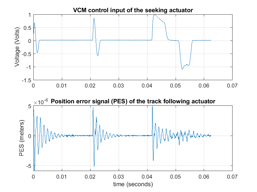
Figure 1: The input and output time series used for the simulations

A total of 1600 measurements were used and $p$ was chosen to be 800. Ten most dominant singular values of the Hankel matrix were used for the estimation which gave a tenth order plant estimate. Fig.3 shows frequency response plots of the actual and estimated plots. The PES collected had more high frequency components and hence a more accurate fit in the high frequency region was obtained.

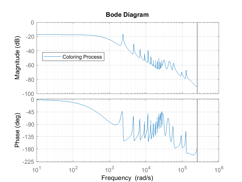
Figure 2: The frequency response plot of the coloring dynamics used for simulations

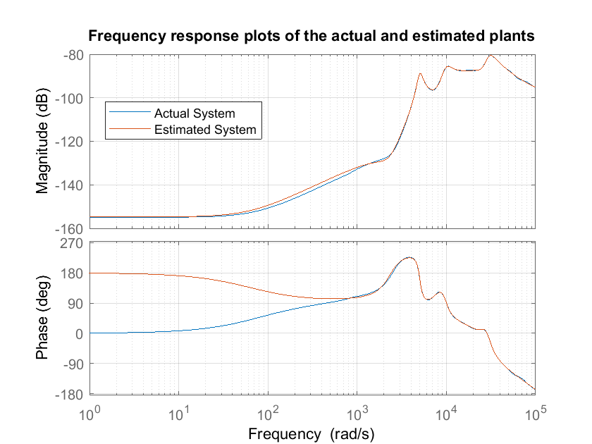
Figure 3: Frequency responses of the actual plant and the estimated plant

V Conclusions

In this paper the OKID/ERA algorithm was extended to include colored noises. The algorithm was used to estimate the disturbance cross transfer function between the voice coil motor input of the track seeking actuator and the output of the track following actuator in a multi actuator hard disk drive.

References

- [1] Jer-Nan Juang, Minh Phan, Lucas G. Horta and Richard W. Longman, "identification of Observer/Kalman Filter Markov Parameters: Theory and Experiments", in Journal of Guidance Control and Dynamics, vol. 16, No.2,March-April 1993.
- [2] W.-K. Chen, Linear Networks and Systems (Book style). Belmont, CA: Wadsworth, 1993, pp. 123–135.
- [3] Francesco Vicario, Minh Q Phan, Raimondo Betti, Richard W Longman, "OKID via Output Residuals: A Converter from Stochastic to Deterministic System Identification", in Journal of Guidance, Control, and Dynamics, vol. 40, Issue 12, 2007, pp. 3226–3238.
- [4] Guojun Sun, Richard W Longman, Raimondo Betti, Zhihua Chen, Suduo Xue, "Observer Kalman filter identification of suspen-dome", in Journal of Mathematical Problems in Engineering, 2017.
- [5] Francesco Vicario, Minh Q Phan, Richard W Longman, Raimondo Betti, "Generalized framework of OKID for linear state-space model identification", in Modeling, Simulation and Optimization of Complex Processes HPSC 2015, Springer, Cham, 2017, pp. 249–260.
- [6] Francesco Vicario, Minh Q Phan, Raimondo Betti, Richard W Longman, "Output-only observer/Kalman filter identification ", in Journal of Structural Control and Health Monitoring, Vol. 22, Issue 5, 2015, pp. 847–872.
- [7] Francesco Vicario, Minh Q Phan, Raimondo Betti, Richard W Longman, "Extension of OKID to Output-Only System Identification", 2014.
- [8] Phan, M. Q., Vicario, F., Longman, R. W., and Betti, R. (November 8, 2017). "State-Space Model and Kalman Filter Gain Identification by a Kalman Filter of a Kalman Filter." ASME. Journal of Dynamical Systems, Measurement, and Control, March 2018; 140(3): 030902. https://doi.org/10.1115/1.4037778
- [9] Lennart Ljung, Keith Glover, "Frequency domain versus time domain methods in system identification", in Automatica, Vol. 17, Issue 1, 1981, pp. 71-86.
- [10] MATLAB. version 9.10.0 (R2016b). Natick, Massachusetts: The MathWorks Inc.,2016.
- [11] Zhang, Qinghua. “Using Wavelet Network in Nonparametric Estimation”, IEEE Transactions on Neural Networks 8, no. 2 , March 1997. https://doi.org/10.1109/72.557660.
- [12] Sjöberg, Jonas, Qinghua Zhang, Lennart Ljung, Albert Benveniste, Bernard Delyon, Pierre-Yves Glorennec, Håkan Hjalmarsson, and Anatoli Juditsky. “Nonlinear Black-Box Modeling in System Identification: A Unified Overview”, Automatica 31, no. 12 (December 1995): 1691–-1724. https://doi.org/10.1016/0005-1098(95)00120-8.
- [13] Ljung, Lennart, and Torkel Glad. Modeling of Dynamic Systems. Prentice Hall Information and System Sciences Series. Englewood Cliffs, NJ: PTR Prentice Hall, 1994.
- [14] Ljung, Lennart. System Identification: Theory for the User. Second edition. Prentice Hall Information and System Sciences Series. Upper Saddle River, NJ: PTR Prentice Hall, 1999.
- [15] Söderström, Torsten, and Petre Stoica. System Identification. Prentice Hall International Series in Systems and Control Engineering. New York: Prentice Hall, 1989.
- [16] Lennart Ljung, "Analysis of recursive stochastic algorithms", IEEE transactions on automatic control 22.4, 1977, pp. 551–575.
- [17] Behrooz Shahsavari, Jinwen Pan, and Roberto Horowitz, "Adaptive rejection of periodic disturbances acting on linear systems with unknown dynamics", IEEE
- [18] Simon Haykin and Bernard Widrow, "Least-mean-square adaptive filters", Vol. 31. John Wiley & Sons, 2003.
- [19] Simon S Haykin, "Adaptive filter theory", Pearson Education India, 2008.
- [20] Roberto Horowitz et al, "Dual-stage servo systems and vibration compensation in computer hard disk drives", Control Engineering Practice 15.3 (2007), pp. 291–305.
- [21] A. Tiano, R. Sutton, A. Lozowicki, W. Naeem,"Observer Kalman filter identification of an autonomous underwater vehicle", Control Engineering Practice, Vol. 15, Issue 6, 2007, pp. 727–739, ISSN 0967-0661, https://doi.org/10.1016/j.conengprac.2006.08.004.
- [22] Juang, J.-N., Pappa, R. S., "An Eigensystem Realization Algorithm for Modal Parameter Identification and Model Reduction", Journal of Guidance, Control, and Dynamics, Vol. 8, Issue 5, pp.620–-627
- [23] H.P.Gavin, "Eigensystem Realization", Course Notes, Duke University, April 15, 2020.