Two Souls in an Adversarial Image: Towards Universal Adversarial Example Detection using Multi-view Inconsistency

Abstract.

In the evasion attacks against deep neural networks (DNN), the attacker generates adversarial instances that are visually indistinguishable from benign samples and sends them to the target DNN to trigger misclassifications. In this paper, we propose a novel multi-view adversarial image detector, namely Argos, based on a novel observation. That is, there exist two “souls” in an adversarial instance, i.e., the visually unchanged content, which corresponds to the true label, and the added invisible perturbation, which corresponds to the misclassified label. Such inconsistencies could be further amplified through an autoregressive generative approach that generates images with seed pixels selected from the original image, a selected label, and pixel distributions learned from the training data. The generated images (i.e., the “views”) will deviate significantly from the original one if the label is adversarial, demonstrating inconsistencies that Argos expects to detect. To this end, Argos first amplifies the discrepancies between the visual content of an image and its misclassified label induced by the attack using a set of regeneration mechanisms and then identifies an image as adversarial if the reproduced views deviate to a preset degree. Our experimental results show that Argos significantly outperforms two representative adversarial detectors in both detection accuracy and robustness against six well-known adversarial attacks. Code is available at: https://github.com/sohaib730/Argos-Adversarial_Detection

1. Introduction

With the growing computational power and the enormous data available from many sectors, applications with machine learning (ML) components are widely adopted in our everyday lives (Kiani et al., 2020). ML models especially deep neural networks (DNNs) now achieve human-level or even better performance in many challenging tasks, such as face/object recognition (Sun et al., 2015; Liang and Hu, 2015), image classification (Rawat and Wang, 2017), autonomous driving (Grigorescu et al., 2020; Muhammad et al., 2020), and playing the game of Go (Silver et al., 2016). Meanwhile, a broad spectrum of cyber-attacks against DNNs such as poisoning (Steinhardt et al., 2017; Shafahi et al., 2018; Awan et al., 2021; Tang et al., 2021), evasion, backdoor (Pang et al., 2020; Liu et al., 2018; Tang et al., 2020), and model inversion (Fredrikson et al., 2015; Wu et al., 2016) has been proposed recently. One of the most harmful attacks is the evasion attack (Madry et al., 2018; Biggio et al., 2013; Nguyen et al., 2015; Szegedy et al., 2013), also known as adversarial examples, in which small imperceptible perturbations are added to input samples. These adversarial instances can fool the victim classifiers to make highly confident but erroneous predictions, and therefore have garnered significant attention from the defense side, e.g., (Song et al., 2018; Metzen et al., 2017; Samangouei et al., 2018; Feinman et al., 2017; Xu et al., 2018).

Existing countermeasures against the evasion attacks could be roughly divided into three categories: (i) to sanitize the input samples to (potentially) eliminate the adversarial perturbations (Song et al., 2018; Doan et al., 2020); (ii) to enhance the robustness of the machine learning models, e.g., through adversarial training (Madry et al., 2018; Cao and Gong, 2017; Cohen et al., 2019); and (iii) to detect the adversarial perturbations and instances  (Metzen et al., 2017; Feinman et al., 2017; Xu et al., 2018). While these approaches have shown their effectiveness in detecting or preventing representative evasion attacks, they still fall short in meeting the expectation for general and practical solutions. In particular, we have observed three key limitations in the state-of-the-art (SOTA) approaches. First, most of the current defenses are designed for black-box attacks, in which the attacker is assumed to know nothing about the defense mechanism (architecture and weights). However, in white-box attacks, the adversary with full knowledge of the victim model and the defense approach can easily generate adversarial examples that can evade the seemingly robust models or escape from detection (Athalye et al., 2018; Carlini and Wagner, 2017a). Second, defenses based on adversarial training achieve better performance against white-box attacks than the other two categories, but they incur an unavoidable penalty to clean model accuracy, as this line of solutions essentially trades classification accuracy for model robustness (Tsipras et al., 2018; Zhang et al., 2019). Moreover, the robustness of such models is still limited in certain cases. For example, for adversarial examples with high perturbations, the accuracy of these approaches drops to 25% or below (Madry et al., 2018). Finally, the SOTA attack detection solutions, especially the feature domain detectors, have shown promising performance in detecting adversarial examples with high perturbations, but many of them perform poorly in the detection of adversarial examples with low perturbations.

In this paper, we present the Argos solution, which attempts to tackle the challenge of adversarial example detection from a novel perspective. Intuitively, we have observed that an adversarial example, regardless of the level of perturbation, contains two inherently contradictory “souls”: (i) the image content that is visually indistinguishable from benign samples, and (ii) the added invisible perturbation that corresponds to an adversarial label. When a victim classifier is misled by the adversarial perturbation, it generates a wrong label for the input adversary instance. We argue that the inherent discrepancy between the visible “clean” content and the misclassified label, which is forced by the invisible adversarial content, could be utilized in detecting adversarial examples. To amplify the discrepancy between the two “souls” to an extent that can be detected, we propose a novel generation-and-detection approach that first adopts an autoregressive generative model to regenerate images (called views in this work) using different sets of seed pixels from the original image and the predicted label (Section 4.2), and then detects the inconsistencies between the original image and the view ensembles as well as across the views with a multi-view detector named Argos (Section 4.3).

The rationale behind this design is two-fold. First, for a clean input, all the views generated with different seeds and the same correct label should be visually and distributionally similar so that the inconsistencies across the views and the original input are very low. On the contrary, a successful adversarial instance that fools the neural network classifier will result in a misclassified label and inevitably cause inconsistencies between the original image and the generated views as we expect. These views are not only significantly different from the original input, but more importantly, different from each other. Therefore, we further develop a novel model to measure and evaluate such inconsistencies for adversarial sample detection. Another advantage of the Argos approach is that it does not rely on any prior knowledge nor make any assumption about the adversarial attack method (as long as the attack is successful). As a result, it can effectively detect unknown attacks.

Our contributions are summarized as follows.

• We are among the first to identify the inherent discrepancy between the (visually) benign content and the misclassified label in a successful adversarial example attack and leverage such discrepancy for attack detection.

• We propose a novel generation-and-detection approach to amplify the imperceptible perturbation with an autoregressive generative model and develop a multi-view detector to measure the (in)consistencies across the generated images for adversarial example detection.

• Through extensive experiments, we show that the Argos detector is highly accurate and robust. Moreover, it significantly outperforms SOTA solutions against the strongest adversarial attacks.

The rest of the paper is organized as follows: We present the threat model in Section 2 and an overview of our solution in Section 3. We present the detailed design of Argos in Section 4, followed by the experimental results and some discussions in Sections 5 and 6. Finally, we briefly summarize the related work in Section 7 and conclude our work in Section 8.

2. Background and Threat Model

2.1. Basic Notations and Objective

We denote benign image as $x$, its true label as $y$, and the corresponding adversarially perturbed image as $x^{\prime}$. We denote input image for classification/detection as $z$, which can be benign or adversarial i.e. $z=\{x,x^{\prime}\}$. We assume that all images have been flatten into $n$-dimensional vectors, i.e., $z\in\mathbb{R}^{n}$. Let $F:\mathbb{R}^{n}\rightarrow\mathbb{R}$ be a deep neural network (DNN) classifier, mapping an input image $z$ to a probability vector $f(z)$, such that predicted label $F(z)=\operatorname*{argmax}(f(z))$. Let $h(z)$ be the vector presentation of $z$ at the penultimate layer of the network. We assume $F$ is standardly optimized from a labeled training set using a loss function $L(\theta)$, where $\theta$ is the set of network weights (to optimize).

Recall $F$ is expected to correctly classify images. Under an attack with $x^{\prime}$, $F$ may give wrong prediction, i.e., $F(x^{\prime})\neq y$. Our goal is to detect $x^{\prime}$ when it launches a successful attack. We propose to build a detector $D:\mathbb{R}^{n}\times\mathbb{N}\rightarrow\{0,1\}$, mapping from an image and its predicted label to a binary variable indicating whether the image is adversarial. If an image $z$ receives $D(z,F(z))=1$, then it is likely an adversarial instance and its predicted label $F(z)$ should be voided or at least alerted.

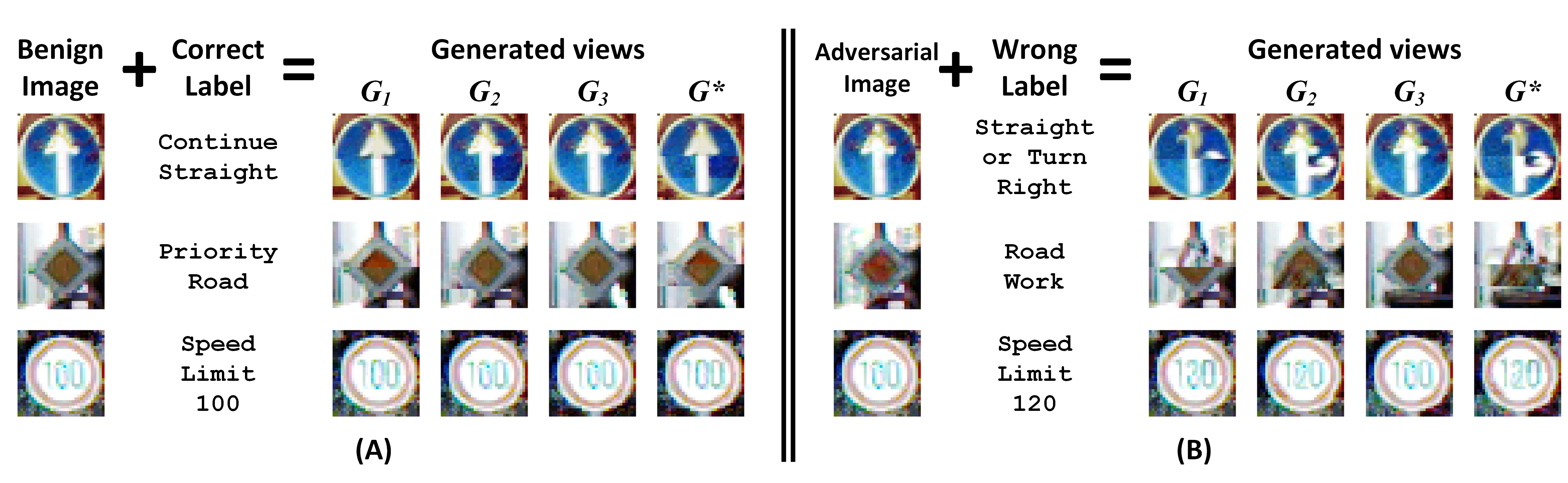
Figure 1. Examples of generated views for benign and adversarial images: each image receives a label from the classifier, four views are generated from the seed image and the label. (A) Benign images; (B) Adversarial images.

2.2. The Threat Model

In this paper, we follow the standard threat model of evasion attacks against deep neural networks. The adversary, acting as a legitimate user of the victim DNN, deliberately introduces adversarial perturbation to $x$ and generates the corresponding $x^{\prime}$, which is visually indistinguishable from $x$. The adversarial example is supposed to be within a certain $L_{p}$ distance from $x$, i.e., $\left\|x-x^{\prime}\right\|_{p}\leq\epsilon$, where $\epsilon\in[0,255]$ is called the perturbation budget.

As introduced above, the victim system has a DNN classifier $F$ and an optional adversarial input detector $D$. Ultimately, the adversary has two objectives that are orthogonal: (Obj-1) to fool the victim DNN to misclassify $x^{\prime}$ to a wrong label (i.e., $F(x^{\prime})\neq y$); and (Obj-2) to fool the adversarial input detector (if it exists) to classify $x^{\prime}$ as benign, i.e., $D(x^{\prime},F(x^{\prime}))$=0.

Prior works in the literature consider two threat models, the black-box (Limited knowledge) and the white-box (Complete knowledge) settings (Carlini and Wagner, 2017a). Both settings assume the attacker has full knowledge of the victim DNN $F(\cdot)$, including all the model parameters/weights, to craft effective adversarial instances. However, the attackers have different knowledge about the detector:

• The black-box setting assumes the attacker has full access to $F(.)$, but does not know anything about the (existence of) detector $D(.)$. In this case, the attacker only attempts to achieve Obj-1.

• The white-box setting assumes the attacker has full knowledge of both the victim DNN and the detector, including all the weights, but not the testing-time randomness. In this case, the attacker attempts to achieve both Obj-1 and Obj-2, as defined above.

From the defense perspective, the detector is expected to work in a semi-autonomous setting, where it only interacts with the DNN owner when an adversarial instance is detected. It has full knowledge of the victim DNN and full access to the training data. We do not make any assumption on the attack method that will be employed to generate adversarial examples. To develop such a general-purpose detector, any assumption made in the design should be generalizable to unknown attacks and the defense mechanism should not rely on a large number of adversarial examples from any specific attack(s). Last, a benign input may be mistakenly classified into a wrong label by the victim DNN, since DNNs cannot achieve 100% accuracy. The misclassified benign inputs are considered outside of the scope of the detector. We briefly compare and discuss the adversarially misclassified samples and naturally misclassified samples in Section 6.

Adversarial Attacks. In this paper, we will evaluate Argos and other adversarial image detectors with the following attacks: Fast Gradient Sign (FGSM) (Goodfellow et al., 2015), Projected Gradient Descent (PGD) (Madry et al., 2018), Momentum Iterative Method (MIM) (Dong et al., 2018), DeepFool (Moosavi-Dezfooli et al., 2016), the Carlini & Wagner (C&W) Attack (Carlini and Wagner, 2017b), and a white-box attack designed by us (to be elaborated in Section 5). A brief introduction to each of the existing attacks could be found in Appendix A. For more details of the attacks, please refer to their original publications.

3. Solution Overview

Intuitively, an adversarial image contains two “souls”: (i) the visible content, which is visually consistent with the clean label; and (ii) the adversarial perturbation, which is invisible but pushes the victim DNN to generate a wrong label. These two “souls” are fundamentally discrepant, while the “stronger” soul will win the competition at the DNN. For a well-crafted adversarial image, a very small perturbation is sufficient to trick the victim DNN to classify it into a wrong label. Conventional adversarial detectors use the added perturbation as a source of information to identify adversarial examples. They fall short in detecting low-perturbation attacks because the added noise is almost imperceptible or against the white box adversaries who control the added perturbation to fool the detector.

The core idea of Argos is to amplify the discrepancy between the visual content of the image and the wrong label that is forced by the invisible perturbation. In particular, we propose to generate different views from a part of the original image (seed pixels) and the predicted label using an autoregressive generative approach. Next, we present two sets of examples that inspire our design.

Observations. In Figure 1 (A), benign images from the GTSRB dataset (Stallkamp et al., 2012) are correctly classified by a deep neural network. We invoke a generative model, namely PixelCNN++ (Salimans et al., 2017), to produce four views ($G_{1}$ to $G^{*}$) from the source images and their predicted labels. Each view ($G_{1}$ to $G_{3}$) was generated using a different number of seed pixels. $G^{*}$ is an integration of the three views (we will discuss the details of view generation in Section 4). As shown in the figure, all four views appear to be similar and visually consistent with the source image. In Figure 1 (B), three adversarial images, which look identical to the benign ones, are sent to the same DNN and receive adversarial labels. We generate four views from the adversarial images and the corresponding misclassified labels. From the figure, we have the following observations: (i) the generated images appear very inconsistent, (ii) both the original image and the adversarial label (i.e., two “souls”) are somewhat reflected in most of the generated images, and (iii) most of the generated images visually deviate from the original image.

Argos Overview. With the observations, we design a multi-view adversarial image detector, namely Argos. As shown in Figure 2, the end-to-end image classification and adversarial example detection approach consist of four steps: (1) An input image $z$, benign or adversarial, is sent to the target DNN, which assigns a label $F(z)$ to the input. We do not know whether the image is clean or adversarial, or whether the label is correct or wrong. (2) Both $z$ and $F(z)$ are sent to a generative model, which creates multiple views ($G_{1},G_{2},G_{3}$ and $G^{*}$) using the label $F(z)$ and different portions of $z$ as seeds. In each view $G_{i}$ in the figure, the region of the image highlighted in the red dashed rectangle is generated. (3) All the views, as well as the original image $z$, are sent to the decision module, which measures the discrepancies among them to determine if the label is benign or adversarial. (4) Finally, based on the output from Argos, we choose to accept the label, or reject the label and raise an alert.

Advantages of Argos. Argos does not make any assumption of the attack method, except the fact that the attacker switches the output label of the adversarial example ($x^{\prime}$) from $y$ to $t$, while $x^{\prime}$ is still visually similar to other samples in class $y$. The view generation mechanism has a single objective, which is to amplify the inconsistency, if any, among the visual content of the image and the predicted label. Therefore, Argos is designed to detect all adversarial examples without distinction. It does not rely on a specific feature or algorithm of the attacks or a specific type or strength of the added perturbation, so that Argos is highly generalizable to known or unknown attacks. It is also more robust against white-box attacks than other approaches (to be demonstrated in Section 5). In addition to adversarial detection, Argos can also identify some misclassified benign samples (to be discussed in Section 6).

4. Argos: the Multi-view Detector for Adversarial Examples

4.1. A Revisit of Conditional PixelCNN

Let $z=(z_{1},...z_{n})$ be an $n$-dimensional vector representation of a flattened image $z$, where all pixels are assumed sorted in the raster scan order, i.e., sorted row by row (from top to bottom) and pixel by pixel within each row (from left to right).

PixelCNN  (Van Oord et al., 2016) is an autoregressive modelling technique that models the joint pixel distribution of $z$ by factoring it into a product of the following conditional pixel distributions:

$$p(z)=\prod_{i=1}^{n}p(z_{i}|z_{1},....z_{i-1}).$$

The right distributions are modeled by a shared convolutional neural network learned from a set of training images.

PixelCNN is widely applied to generate diverse images that are capable of capturing the high-level structure of the training images (Uria et al., 2016). In practice, it generates an image by selecting its first $k$ pixels (called seeds) and generating the rest one by one, with the $i_{th}$ pixel randomly sampled from

(1) $$p(z_{i}\mid z_{1},\ldots,z_{i-1}).$$

Conditional PixelCNN (Oord et al., 2016; Salimans et al., 2017) is an enhanced version of pixelCNN which further conditions each pixel distribution on a given label $\hat{y}$ (not necessarily $y$), with an aim of improving the visual quality of the generated images, i.e., it models

(2) $$p(z\mid\hat{y})=\prod_{i=1}^{n}\,p(z_{i}|z_{1},....z_{i-1},\hat{y}).$$

In this paper, we discover a new application of the above label dependence for detecting adversarial image $x^{\prime}$. By setting $\hat{y}=F(x^{\prime})$, we show (2) can be applied to generate low-quality copies of $x^{\prime}$, based on the inconsistency between its visually unchanged content (i.e., $||x-x^{\prime}||_{p}\leq\epsilon$) and mis-classified label (i.e., $F(x^{\prime})\neq y$). We hypothesize that such inconsistency can be leveraged to detect adversarial images.

4.2. View Generation and Ensemble

Given a test image $z$, we first generate a copy of it, denoted by $G(z,F(z))$, using conditional pixelCNN based on both $z$ and $F(z)$. Intuitively, if $z$ is a successful adversary, it should visually look like one object but be classified as another. In the experiment, we observe such inconsistency being amplified in the generated copies. In this paper, we have denoted generated image as $G$ and omitted it’s input $(z,F(z))$ to save space.

Let us re-visit Figure 1 that shows two sets of results: in (A), the generated copies of three benign images are conditioned on correctly predicted labels. In each row, the left-most column shows the test image and the following columns show the generated copies using different sets of seeds. And in (B), the generated copies of three adversarial images are conditioned on misclassified labels.

Take the top image in (B) as an example. The input image is undoubtedly a ‘go-straight’ sign by appearance, but is actually an adversarial image misclassified as ‘go-straight-or-turn-right’. Then, we see the first generated copy $G_{1}$ looks like an integration of go-straight and go-straight-or-turn-right, which deviates significantly from the input image. While similar observations can be found for the other two adversarial examples (the ‘Road Work’ sign in the second row and the ‘Speed Limit 120’ sign in the third row), we do not see such deviation in benign images in (A). This implies that the inconsistencies between the visual features and the misclassified labels can be re-captured and used to detect adversarial images.

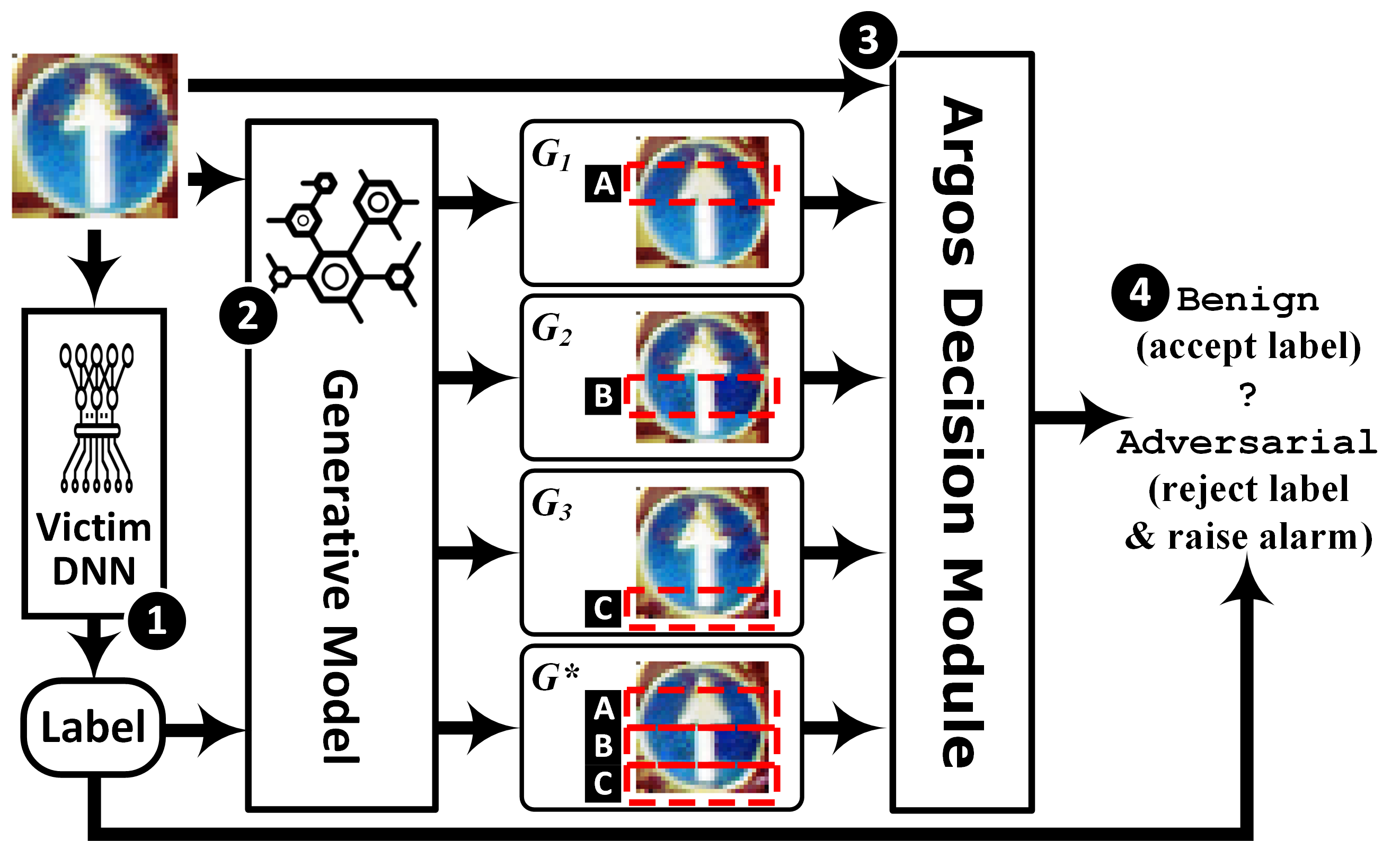
Figure 2. An Overview of the Argos approach.

To generate a copy $G$ of a test image $z$, a naive way is to select the first $x$ pixels (horizontally or vertically) of $z$ and generate the rest using Eq. (2). However, there could be many different approaches to select the seeds and the generated portion of the image. The view generation strategy in Argos is mostly empirical. We have observed that a top-down approach generates better views for benign images. Meanwhile, we also observed that the quality of the generated rows of pixels will decrease when the new rows are far away from the seeds, as their sampling distributions are conditioned heavily on the previously generated pixels, instead of the observed seeds. This may add noise even for benign images and consequently lower the detection accuracy. To mitigate this issue, we only generate a small portion of the image in each copy $G$, and adopt the remaining pixels from the original input image. Since we do not know where exactly the object is located in the image, we generate multiple copies of $z$, each called a view ($G_{k}$) with each focusing on a different area of the image. To capture the overall effect, the final view $G^{*}$ is assembled from all the generated pixels from previously generated views.

In Argos, the $k_{th}$ view $G_{k}$ is created by taking the first $m_{k}$ rows of pixels in $z$ as seeds to generate rows ranging from $(m_{k}+1,m_{k+1})$. For an image with $n$ number of rows we set $m_{k}$ = $k\times\frac{n}{4}$. Thus, we generate a quarter of an image in each view which gives three $G_{k}$ views and the final view $G^{*}$ is assembled from the generated rows from all $G_{k}$ views. Among all the views, the area that was not filled by generated rows will be copied as is from the input image $z$. For instance, with an input image of 32$\times$32 pixels, we have $m_{1}$=8, $m_{2}$=16, and $m_{3}$=24. As shown in Figure 2, in view $G_{1}$, rows 9 to 16 are generated with Eq. (2) (labeled as in Figure 2), while all other rows are directly adopted from $z$. In the same way, rows 17 to 24 are generated in $G_{2}$ ( in Figure 2), and rows 25 to 32 are generated in $G_{3}$ ( in Figure 2). Finally, view $G^{*}$ adopts the generated regions from $G_{1}$ to $G_{3}$ to generate an integrated view.

In practice, $G_{k}$ views may be generated in parallel to improve the computational efficiency of Argos. More efficient implementations of PixelCNN (Ramachandran et al., 2017; Guo et al., 2017; Xu et al., 2021) can also be used to further speed up the auto-regressive generation procedure. In the current implementation of Argos, we adopt the fast pixelCNN from (Guo et al., 2017).

The view generation approach described above is static and does not vary from sample to sample. Whereas, the region of interest during view generation is the object location, and for each input sample it will be different. Currently, in static approach we generate three views with the expectation that object will be located in any one of them. On the other hand, if object location is known beforehand, in theory Argos will only generate views that cover the object. However, problem with this approach is the white-box adversary may fool the algorithm that identifies region of interest. It is our future plan to explore and employ object localization approaches that are robust against white-box attacks. The localization approach need to be unsupervised for wider applicability and for Argos we only need rough estimate of object location.

4.3. Adversary Detection

For adversarial detection, we have used four metrics to make our detector robust against different types of attacks. The metrics are discussed below. Our fundamental approach is to measure the inconsistency between an input image and its corresponding generated views. The intuition is that while the features learned by a classifier are a combination of both robust and non-robust features, the adversary can only tamper with the non-robust features to induce a misclassification of the target label (Ilyas et al., 2019). With the generative approach and the predicted label, Argos  maps the robust features of the adversarial content (e.g., the object corresponding to the adversarial label) into generated views. Specifically, among the generated views, $G^{*}$ is more likely than others to capture the robust features of two distinct objects. Moreover, for an adversary example whose likelihood distribution $P(x^{\prime})$ is lower than benign images, the generated pixels will be erroneous which means perturbation will be propagated in auto-regressive generative process.

Predictors. The first metric measures the euclidean distance between the representation vectors of input image z and its generated view $G^{*}$, i.e:

(3) $$D_{1}(z)=||h(z)-h(G^{*})||_{2}$$

$D_{1}(z)$ is especially effective in detecting aggressive attacks that adds high perturbations.

The second metric measures the distance in probability space with Kullback-Leiber(KL) divergence (Joyce, 2011) using output probability vector $f(.)$ of input image $z$ and its generated views $G_{i}$:

(4) $$D_{2}(z)=\sum_{i=1}^{3}\operatorname{KL}(f(z),f(G_{i}))+\operatorname{KL}(f(z),f(G^{*}))$$

$D_{2}(z)$ is highly effective when the added perturbation is small.

The third metric is adopted from existing literature that only uses a single view i.e., the detector of PixelDefend (PD) (Song et al., 2018). It leverages the likelihood distribution of the input images to identify adversarial images. Since our view generation approach already leverages the likelihood distribution of images, the incorporation of this metric is straightforward:

(5) $$D_{3}(z)=P(z)$$

The fourth metric is adopted from literature, i.e., the I-defender (ID) (Zheng and Hong, 2018), which only uses the class conditional likelihood distribution of the classifier’s representation layer $h(z)$ learned with the class conditional Gaussian mixture model (GMM):

(6) $$D_{4}(z)=P(h(z)|F(z))$$

Since, it’s obvious all four metrics are determined for particular image $z$, we will omit $z$ and use notation $D_{i}$.

In previously proposed approaches (Cohen et al., 2020; Song et al., 2018; Zheng and Hong, 2018), a single metric was preferred to completely avoid training. However, it’s difficult to guarantee general robustness due to varying nature of attacks (Tramèr et al., 2020). Based on our observation, different attacks have varying impacts on the metrics $D_{1}$ to $D_{4}$. Roughly, we can divide the attacks into three categories: (i) the stealthier attacks with low perturbations, (ii) the aggressive attacks with high perturbations, and (iii) the defense-aware attacks (i.e., white-box attacks). We incorporated four metrics into our detection scheme that can counter all attacks effectively. To evaluate the importance of the above-mentioned predictors ($D_{1}$ - $D_{4}$) in detecting several representative attacks, we plot the mutual information (MI) between each predictor and detection label in Figure 3. As shown in the figure, the predictor $D3$ is effective against aggressive attacks like CW and iterative Linf-based attacks (MIM,PGD) but it is ineffective against DeepFool that is known to add small perturbations. Similarly, the metric $D_{4}$ is ineffective against iterative attacks (MIM, PGD). While each metric $D_{3}$ or $D_{4}$ is only effective against a certain type of attack and neither performs well against white-box attacks. However, newly proposed metrics $D_{1}$ and $D_{2}$ provide complementary information to $D_{3}$ or $D_{4}$ to boost the detection performance, and are also effective against white-box attacks (See Table 4). For instance, $D_{1}$ is very effective in detecting white-box and iterative MIM attacks. Whereas, $D_{2}$ is more effective in detecting small added perturbations, e.g., in DeepFool attack.

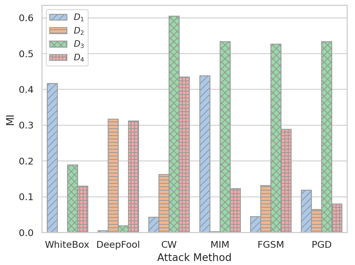
Figure 3. Feature Importance for detection against various attacks. MI: mutual information.

The Detector. Finally, the Argos detector utilizes all four predictors $d(z)=(D_{1},D_{2},D_{3},D_{4})$ in adversarial image detection. The objective of the detector design is to make it effective against different types of attacks, including potentially unknown attacks, with minimum training effort. We can observe from Figure 3 that feature importance varies among different attacks and creates a covariate shift problem. Therefore, a supervised model trained with samples specific to one attack may be ineffective against other attacks.

In Argos, we adopt a hybrid of a supervised detector and a novelty detector. We observe certain patterns in the predictor feature importance with the representative attacks. As shown in Figure 3, the detection of aggressive attacks like CW and L-inf based (MIM, FGSM, PGD) rely on all four features to a certain degree with metric D3 being the dominant one. The other extreme is attacks that add small perturbations such as DeepFool, whose dominant features are different. Therefore, we adopt a supervised Random Forest (RF) (Statistics and Breiman, 2001) classifier with $K$ trees and train it using adversarial samples only from DeepFool and PGD ($\epsilon=4$). Meanwhile, a Novelty detector, Isolation Forest (IF) (Liu et al., 2008), is trained using only the benign samples. The supervised detector identifies most of the (known) black-box attacks, while the novelty detector suffices for detecting white-box attacks, including potentially unknown attacks.

In detection, the final outcome of the hybrid detector is “benign” ($D(z,F(z))=0$) if both supervised and novelty detector are confident to classify $z$ as benign, otherwise, the output label is “adversarial” ($D(z,F(z))=1$).

(7) $$D(z,F(z))=\left\{\begin{matrix}0&P_{RF}(y^{\prime}=0)+P_{IF}(y^{\prime}=0)>\tau.\\ 1&\text{otherwise}\\ \end{matrix}\right.$$

where $\tau$ is the fixed threshold and $y^{\prime}$ is the output of RF and IF,

$$\begin{split}&P_{RF}(y^{\prime}=0)=\frac{\sum_{k=0}^{K}\mathbb{I}(t_{k}(d(z))=0)}{K}\\ &P_{IF}(y^{\prime}=0)=2^{\frac{-E(t(d(z)))}{c}}\end{split}$$

$P_{RF}(y^{\prime}=0)$ is the proportion of Trees $t_{k}$ in RF, classifies $d(z)$ as ’benign’ and $\mathbb{I}$ is the indicator function. $P_{IF}(y^{\prime}=0)$ is the anomaly score of IF in which $t(d(z))$ is the path length of observation $d(z)$, $c$ is the average path length of unsuccessful search in a Binary Search Tree. We prove empirically that such detection scheme generalizes well across different kinds of attacks (See Table 2).

5. Experiments

In this section, we present the adversarial example detection performance of Argos against six different attacks on three datasets. We compare Argos with two adversary detectors in the literature, and further analyze the performance of these approaches.

5.1. Experiment Setup

Datasets. We evaluate Argos on three datasets: the German Traffic Sign Recognition Benchmark (GTSRB) (Stallkamp et al., 2012), the R-ImageNet (R-ImageNet) (Russakovsky et al., 2015), and CIFAR10 (Krizhevsky, [n.d.]). The dimension of images are fixed as 32 by 32. Adversarial sample defense for the whole ImageNet dataset is known to be a challenging problem, both due to the hardness of the learning problem itself, as well as the computational complexity. R-ImageNet is a subset of the original ImageNet dataset, which is used in other defense literature as well, e.g., (Tsipras et al., 2018; Ilyas et al., 2019), to give similar complexity but with lesser number of samples/classes. On each data set, we use its default split of training, validation, and testing data. The numbers are presented in Table 1.

One important difference among the datasets is the level of complexity for the generation process. For instance, in the GTSRB dataset, object shapes and orientations remain the same across all the samples and there is little background. In CIFAR, object shapes and orientations change among samples with different backgrounds. In R-ImageNet, along with different object shapes, orientations, backgrounds, the added complexity is the similarity between different labels. From the classifier performance demonstrated in Table 1, we can see that the classification accuracy of R-ImageNet is only at 74%. Note that the classification accuracy of each victim classifier is listed here as a reference, it does not impact the detection performance of Argos. For a fair comparison with other approaches, it is important that the same datasets are used across all the experiments. We deliberately select a complex susbset to demonstrate the limits of Argos and other adversarial sample detectors.

Metrics. We adopt three metrics that are widely used in the literature: (i) the attack detection rate (ADR) of an adversarial example detector is defined as the proportion of correctly detected adversarial samples out of all adversarial samples, i.e., the recall of adversarial examples or the true positive rate (TPR); (ii) the benign detection rate (BDR) is the proportion of correctly labeled benign images out of all benign images, i.e., the true negative rate (TNR); (iii) we also use the standard ROC curve and AUROC score to evaluate the true positive rate (TPR) with varying false positive rates (FPR=1-TNR).

Table 1. Datasets and performance of the base models

	No. of	Train/Val/Test	Classifier	NLL
	Classes	Samples	Accuracy	(bits)
GTSRB	43	39,209/2,630/10,000	98%	1.7
R-ImageNet	16	40,517/400/1200	74%	4.60
CIFAR10	10	45,000/5000/10,000	95%	2.94

Table 2. Performance comparison: the Attack Detection Rate (evaluated with fixed TNR=95%) and AUROC score of Argos (ours), I-Defender (Zheng and Hong, 2018), and PixelDefend (Song et al., 2018). Both scores are scaled to [0, 100]. SR: Attack Success Rate.

	GTSRB							CIFAR-10							R-ImageNet
		Detection Rate			AUROC				Detection Rate			AUROC				Detection Rate			AUROC
Attack-$\epsilon$	SR	ID	PD	Ours	ID	PD	Ours	SR	ID	PD	Ours	ID	PD	Ours	SR	ID	PD	Ours	ID	PD	Ours
DeepFool	94	68	47	92	90	85	98	96	53	14	58	90	59	92	100	29	8	42	79	55	87
CW: 0.5	66	60	73	97	89	91	99	87	83	98	99	95	99	99	98	24	77	70	72	94	91
PGD-4	-	-	-	-	-	-	-	95	23	98	91	73	98	97	76	16	15	42	64	74	79
PGD-8	57	32	84	86	82	96	98	96	23	99	99	74	99	98	91	17	46	64	65	89	87
PGD-16	90	38	99	88	84	99	99	96	24	99	99	75	99	98	92	21	96	84	69	98	95
MIM-4	-	-	-	-	-	-	-	90	28	98	98	76	98	99	77	18	19	51	65	75	79
MIM-8	52	32	79	86	82	95	99	96	45	99	99	85	99	99	91	23	34	71	71	84	88
MIM-16	87	38	97	88	83	99	99	96	54	99	99	89	99	99	92	23	34	72	71	84	89
FGSM-4	-	-	-	-	-	-	-	74	63	96	99	90	98	98	55	23	40	48	71	81	79
FGSM-8	-	-	-	-	-	-	-	82	85	99	99	95	99	99	78	29	73	75	73	94	92
FGSM-16	48	61	88	96	90	97	99	86	96	99	99	97	99	99	87	41	95	89	80	98	96
WB	89	33	38	86	80	85	97	90	1	13	71	31	70	91	96	1	3	45	18	45	71

Victim Model and Training. We use the Wide Residual Network (w-ResNet) (Zagoruyko and Komodakis, 2016) as the target classifier, which the adversarial examples aim to fool. Its testing accuracy against benign samples is presented in Table 1. Meanwhile, two generative models are trained for Argos: (1) PxelCNN++ (Salimans et al., 2017) is employed to learn class conditional input distribution $P(z|y)$ for view generation. Its performance is measured by the average natural log-likelihood (NLL) given as bits per dimension, which is also presented in Table 1. (2) A Gaussian Mixture Model (GMM) with eight components learns the class conditional distribution of the representation, i.e. $P(h(z)|y)$. Finally, we trained Argos  using validation samples and reported detection performance on test samples.

The Failed attacks. When an adversarially modified image fails to trigger misclassification, it is a failed attack. For instance, an adversarial example may fail if the target model is robust or the added perturbation is too low. As shown in Table 2, the success rates (SR) of adversarial attacks range from 100% (DeepFool on R-ImageNet) to 48% (FGSM with $\epsilon=16$ on GTSRB) or even lower (FGSM-4 and FGSM-8 on GTSRB, PGD-4 on GTSRB, etc). In this paper, we do not consider failed attacks in calculating the detection rates, which is a common practice in the literature.

5.2. Experiment Design

To evaluate Argos we generated adversarial examples based on two threat models presented in Section 2.1.

The Black-box Attacks: The black box attack methods involved in our experiments are explained in Appendix A. We have used cleverhans implementation to generate these attacks (Papernot et al., 2018). For each attack method, all adversarial examples were limited by the maximum allowed perturbation i.e. $\left\|x-x^{\prime}\right\|_{p}\leq\epsilon$, where $\epsilon\in[0,255]$. For attack methods whose distance metric is $L_{\infty}$, e.g., FGSM, PGD, and MIM, the added perturbation is controlled by $\epsilon$. On the other hand, among the attack methods that use $L_{2}$ metric, DeepFool ensures to add the smallest perturbation by design, while perturbations in C&W could be controlled by the confidence parameter [0.1,0.9]. In our experiments, adversarial examples are generated with the default settings in DeepFool. C&W attacks are generated with a confidence parameter of 0.5. Three perturbation levels $\epsilon=4,8,16$ are used for PGD, MIM, and FGSM.

The White-Box Attack: In order to generate a white-box attack against Argos, we design a method based on the adaptive techniques described in (Zheng and Hong, 2018; Carlini and Wagner, 2017a; Tramèr et al., 2020). Argos uses generated samples to perform detection based on predictors given in Eq. 3 to 6. For white-box attack, first two predictors given in Eq. 3, 4 can not be controlled since there is no direct access to the generated views. However, it can be ensured that $P(x^{\prime}|F(x^{\prime}))$ stay high like clean examples. Similarly, it can be ensured $P(h(x^{\prime})|F(x^{\prime}))$ remains high i.e. closer to benign samples. We use Iterative $L_{\infty}$ attack with perturbation level $\epsilon=8$ to maximize the following function for $x$:

(8) $$\underset{x}{\operatorname{argmax}}[J(\theta,x,y_{t})+\alpha\prod_{k\neq t}\operatorname{Reject}_{1}(x,y_{k})\times\underset{k\neq t}{max}\log P(x|y_{k})\\ +\beta\prod_{k\neq t}\operatorname{Reject}_{2}(x,y_{k})\times\underset{k\neq t}{max}\log P(h(x)|y_{k})]$$

where the first term $J(.)$ denotes the cross-entropy loss of classifying $x$ into its true label $y_{t}$ by a classifier with parameter $\theta$. This term encourages finding a perturbation that leads to misclassification. The second term penalizes $x$ if its likelihood score from any other classes is lower than the score of the clean sample from the true label. This term encourages $x$ to attain a high likelihood probability with the false label. Similarly, the third term encourages $x$ to attain a high likelihood distribution of the representation vector with the false label. Other possible way to generate white-box attack is using optimization based method (Carlini and Wagner, 2017b). We have observed that Argos is effective against both iterative and optimization based black-box attacks. We expect that if it also works for iterative white-box attack, it will work for optimization based white-box attack as well, since objective remain same in both methods.

5.3. Experimental Results

In this section, we report the experimental results of Argos against the six attacks on three datasets, and compare them with I-Defender (ID) (Zheng and Hong, 2018) and PixelDefend (PD) (Song et al., 2018).

Detection Rate and AUROC. We first evaluate the adversarial example detection rate (ADR) of all three approaches at a fixed TNR of 0.95. The experimental results are reported in Table 2. We also evaluate the AUROC score in each attack and present the results in the same table. We do not evaluate PGD and MIM with $\epsilon=4$, or FGSM with $\epsilon=4,8$ on GTSRB since their attack success rates are too low (¡¡40%) to be practical.

The best performance for each experiment is shown in bold. Argos performs the best (including ties) in 49 out of 64 experiments. Argos’ overall average ADR across all experiments is 80.7%, while the overall average ADR of ID is 37.7% and the average ADR of PD is 67.4%. The average AUROC score of Argos is 0.934, while the average AUROC scores of ID and PD are 0.765 and 0.886, respectively.

We highlight the severe detection failures in red in Table 2, as they are the most destructive cases in practice where detection rates drop below 50%. In particular, the two SOTA detectors can only identify 1% to 3% of the white-box attacks on the R-ImageNet data set and 1% to 13% on the CIFAR-10 data set. Comparatively, Argos manages to identify 45% on R-ImageNet and 71% on CIFAR-10, a substantial improvement over the literature. Besides, the two prior detectors have 23 and 12 severe failures respectively distributed in all three datasets, while Argos only has 4 in R-ImageNet dataset, among which it still achieves the best performance. This demonstrate the outstanding robustness of Argos in worst-case scenarios.

Overall System Performance. The overall accuracy of a classifier+detector system (Figure 2) is defined as the proportion of correctly classified samples and correctly identified adversarial samples out of all inputs. For classifier+detector, there exist a trade off between drop in performance for benign examples and gain in performance for adversarial examples. We have set Argos TNR = 95%, to allow 5% performance drop for benign samples.

Without a detector for adversarial examples, the classification accuracy is the portion of failed attacks that are correctly classified over all attacks. With the existence of Argos, a significant portion of the attack samples are detected. Table 3 presents the classification accuracy of the victim DNN against adversarial samples, and the overall classification+detection accuracy of the DNN+Argos against the same input. Across all the experiments, Argos raises the system accuracy from 14.0% to 81.3%.

ROC. Finally, we evaluate Argos against the attacks that are most difficult to detect: (1) DeepFool; (2) PGD with $\epsilon$=4; (3) C&W; and (4) the white-box attack. To better demonstrate Argos detection accuracy over varying thresholds, we present the ROC curves in Figure 4. We can clearly see that Argos provides solid performance even against the strongest or most stealthy attacks in GTSRB and CIFAR-10 datasets. The performance in R-ImageNet is not as impressive but it’s quite good given the complexity of the dataset.

Ablation Study. In Table 4, we present detection performance for the CIFAR10 dataset by using different combinations of the predictors presented in Section 4.3. Although a single predictor has the advantage that it is easier to adjust the threshold value, we observe from the results in Table 4 that good generalization can not be guaranteed using a single predictor–the AUC scores suffer by a wide margin compared to the best performances, which are achieved using a combination of predictors. For instance, $D_{1}$’s performance against DeepFool is $54\%$, which is much lower than the best performance, $92\%$, which is achieved with $D_{1}$, $D_{2}$ and $D_{4}$.

The high performance across all attacks is guaranteed when all four predictors are used. However, we note that there are also a couple of three-predictor configurations, such as $(D_{1},D_{2},D_{3})$ and $(D_{1},D_{3},D_{4})$, whose performance stays consistently high (in the close vicinity of the best performance) among all attacks. In this case, it is possible to utilize the combination of $D_{1}$, $D_{2}$ and $D_{3}$ for efficiency, as $D_{4}$ requires training of another generative model.

Detection Throughput. On a single node of Nvidia TITAN Xp GPU, Argos  takes approx. 107 seconds to process 100 images. The major bottleneck in throughput is the autoregressive generative process. which generates the three base views, i.e. $G_{1}-G_{3}$. Since all three views are independent, they can be generated in parallel if more computational nodes are available, which will eventually speed up the computation by three folds approximately.

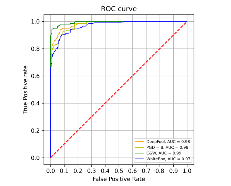
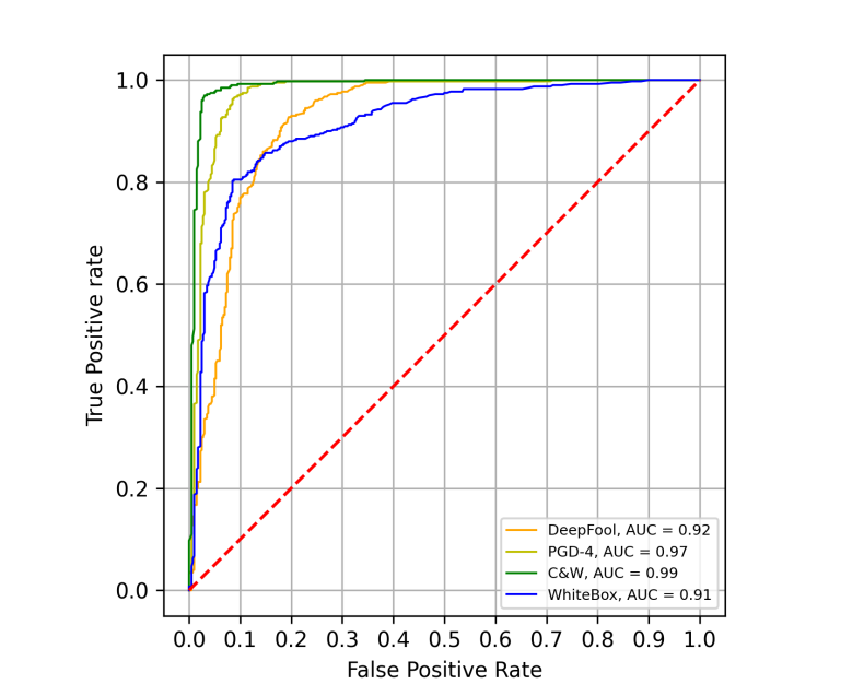
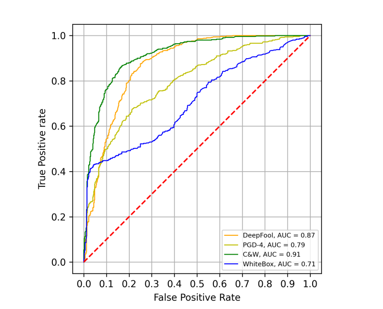
(a)	(b)	(c)

Figure 4. ROC Curves against white box and small perturbation attacks: (a) GTSRB, (b) CIFAR-10, (c) R-ImageNet.

Table 3. System accuracy against adversarial inputs.

DNN: classification accuracy of the the victim DNN;
+Argos: accuracy of DNN+Argos  (adversarial labels are rejected).

	GTSRB		CIFAR-10		R-ImageNet
Attack-$\epsilon$	DNN	+Argos	DNN	+Argos	DNN	+Argos
DeepFool	5.9	92.1	3.8	59.3	0.0	42.0
CW: 0.5	33.3	95.7	12.4	97.9	1.5	70.0
PGD-4			4.8	91.2	17.8	48.8
PGD-8	42.1	89.1	3.8	98.7	6.7	64.6
PGD-16	9.8	88.5	3.8	98.7	5.9	82.9
MIM-4			9.5	97.2	17.0	55.4
MIM-8	47.0	89.4	3.8	98.7	6.7	71.0
MIM-16	12.7	88.7	3.8	98.7	5.9	71.9
FGSM4			24.7	96.7	33.3	58.0
FGSM8			17.1	97.4	16.3	74.0
FGSM16	51.0	94.5	13.3	97.8	9.6	86.6
WB	10.8	86.8	9.5	72.9	3.0	46.0

Table 4. AUC(%) Detection performance of different predictors on CIFAR-10

Predictors				Attacks
$D_{1}$	$D_{2}$	$D_{3}$	$D_{4}$	DF	PGD-$\epsilon_{4}$	CW	WB
$\checkmark$				54	77	67	93
	$\checkmark$			84	64	73	53
		$\checkmark$		59	98	99	70
			$\checkmark$	90	73	95	31
$\checkmark$	$\checkmark$			87	73	76	87
$\checkmark$		$\checkmark$		55	99	99	87
$\checkmark$			$\checkmark$	86	78	95	78
	$\checkmark$	$\checkmark$		85	96	99	58
	$\checkmark$		$\checkmark$	91	74	94	42
		$\checkmark$	$\checkmark$	84	97	90	40
$\checkmark$	$\checkmark$	$\checkmark$		87	97	99	85
$\checkmark$	$\checkmark$		$\checkmark$	92	79	93	81
$\checkmark$		$\checkmark$	$\checkmark$	85	98	99	80
	$\checkmark$	$\checkmark$	$\checkmark$	91	96	91	51
$\checkmark$	$\checkmark$	$\checkmark$	$\checkmark$	92	97	99	91

5.4. Analysis of Experiment Results

Attack Performance. When we compare the attack performance across three datasets, the attack success rates are generally affected by two factors: the complexity of the images and the distance between images from different categories. Attacks on GTSRB are the least successful since images in this dataset are relatively simple–each image has a clear traffic sign in the center and very little background. Moreover, images in each class are quite distinctive from images in other classes. As a result, the image classifier achieves 98% accuracy on this dataset while evasion attacks are difficult. In particular, PGD, MIM and FGSM attacks with low perturbation (e.g., $\epsilon=4$) achieve very low ASRs.

Detection Performance. Compared with SOTA adversarial image detectors, Argos generates higher adversarial detection performance against almost all the attacks and datasets. In particular, for datasets like GTSRB and CIFAR-10 whose classification accuracy is higher, Argos demonstrates superior performance ( 90% ADR). The classification task is simpler when different classes are distinct from each other, which means the two “souls” that Argos exploits for detection are far apart. The results with CIFAR also demonstrate that Argos is not limited by the complexity of images like different object positions, shapes, orientations, and backgrounds. The only limitation comes when the two “souls” of the benign and adversarial labels are not quite different, e.g., an adversarial “truck” image mislabeled as “automobile”. This is the reason why Argos perform comparatively lower in R-ImageNet dataset, as even the classifier is struggling to differentiate the objects for benign images.

Generative Models. The class conditional distribution of representation vector $P(h(x)|y)$ is used to identify adversarial samples in (Lee et al., 2018) and I-Defender (Zheng and Hong, 2018), since the representation of each sample in one class resides in close vicinity to form a group, but the representation of the adversarial samples may not belong to any group. This approach is especially effective against the DeepFool attack that add very small perturbations to push the representation of the adversarial samples towards the target class to trigger misclassification, while the perturbation is not strong enough to push the representation to the close vicinity of the benign samples of the target group. However, this approach cannot guarantee similar performance with more aggressive and white-box attacks, which attempt to push the the adversarial samples to the target group.

On the other hand, PixelDefend (PD) (Song et al., 2018) uses the distribution of input samples $P(x)$ to identify adversarial samples. Like other approaches (Metzen et al., 2017; Samangouei et al., 2018) that use input images for detection, PD is ineffective when the added perturbation is small. Overall, the generative models used in detection are ineffective against white-box attacks since the adversary can ensure high likelihood distribution for the adversarial samples. The major difference in our approach is that we use generative models for view generation instead of likelihood estimation to incorporate predicted label information effectively.

Last, the R-ImageNet is the most complex dataset in our experiments. The complexity in the dataset also introduces additional difficulties in the generative model. As a result, all the generative-model-based detectors perform worse on R-ImageNet data.

6. Discussions

The Interpretability of Argos. In Argos, the predictors $D_{1}$ to $D_{4}$ are used to highlight inconsistencies between the seed image and the views (Section 4.3). The detection properties of these hand-picked predictors are beneficial for three reasons as compared to using a DNN as a detector: (1) The proposed detector in Section 4.3 is more interpretable than a neural network-based model. The response of the adversarial examples to the predictors may give us an insightful understanding of the attacks. (2) Each of the predictors’ outputs can be interpreted as a distance metric which is small for benign samples but increases as the adversarial perturbations increase. Thus, a one-class classifier can be used in conjunction with these predictors for adversarial detection. On the other hand, training a supervised classifier would only require adversarial examples that lie close to decision boundary (i.e. attack samples that add the smallest perturbation) while the classifier would work well as perturbation increases. While we can certainly employ a multi-view classification model for this task, a significant amount of captured or synthetically generated adversarial samples will be needed in training which still cannot guarantee similar performance against unknown attacks. And (3) we intentionally choose a simple detector to highlight the effectiveness of the generation-and-detection approach that amplifies image-label discrepancies and the effectiveness of the novel concept of adversarial detection using multi-view inconsistency. Experiment results have shown that a relatively simple detector is capable of effectively detecting adversarial examples.

Generalization and the White-box Attack Revisited. As we have discussed in Section 3, Argos does not make any assumption of the attack method, except the fact that the visual content of the testing image and the label it receives are inconsistent. In our experiments, when Argos is trained using only the adversarial examples from DeepFool and PGD-4, we see in Table 2 that it generalizes well for all attacks including white-box attacks, which implies that: (1) although the supervised detector is only trained with two attacks, it is capable of detecting a wider range of attacks; and (2) the novelty detector, as a part of Argos, plays a significant role in identifying and mitigating unknown attacks.

When the defensive mechanism against evasion attacks makes any assumption on the attack method, a white-box attack could always be designed to challenge the assumption and thus produce highly successful attacks. To defend against white-box attacks, the only reliable assumption one could make is that the attacker’s goal is to trigger misclassification. Therefore, we incorporate the classified label from the DNN in the design of the detection algorithm. Intuitively, we can simply learn the conditional likelihood distribution $p(x|y)$ and expect $p(x|\text{Correct Label})>p(x|\text{Adversarial Label})$. However, this would not perform well due to the high dimensionality and complexity of image data, as shown in (Van Oord et al., 2016). In Argos, we employ the autoregressive generative models to construct views and sample the conditional probability distributions from there.

Table 5. Detection accuracy (AUC(%)) of misclassified benign vs. adversarial samples.

	Misclassified Benign		Adversarial
Detector	CIFAR	R-ImageNet	CIFAR	R-ImageNet
Argos	83.8	74.2	97.1	85.1

Detection of Misclassified Benign Samples. By design, the predictors $D_{1}$ and $D_{2}$ in Argos exploit the misclassified label in order to detect the adversarial samples. Using the same principle, the predictors are supposed to be effective in identifying misclassified benign samples (a.k.a., naturally misclassified samples). As shown in Table 5, Argos is able to detect approximately 75% to 83% of naturally misclassified samples. This phenomenon of detecting misclassified benign samples by adversarial detector is common in other detection approaches as well (Zheng and Hong, 2018; Vacanti and Looveren, 2020). In safety-critical applications, it is desired if the adversarial detector works in a semi-autonomous fashion and reports all types of misbehaviors (Metzen et al., 2017).

In Argos, we only make one assumption of the input image and label: there exists an inherent discrepancy between the visual content of the image and the label, so that Argos could further amplify and assess such discrepancy for adversarial image detection. This assumption is guaranteed to be true for all successful attack images. Meanwhile, this assumption is also true for a portion of the naturally misclassified images. However, the fundamental difference between naturally misclassified samples and adversarial samples is that the naturally misclassified samples are more likely to carry visual features akin to the wrong label, so that the image-label discrepancies are low. Figure 5 demonstrates two misclassified benign samples from the CIFAR dataset. The tanker truck in the first image has a metal tank that is visually similar to a wing of an airplane (the misclassified label). Therefore, the generative model was able to produce reasonably consistent “airplane” views from the source image. As a result, Argos was unable to detect this misclassified sample.

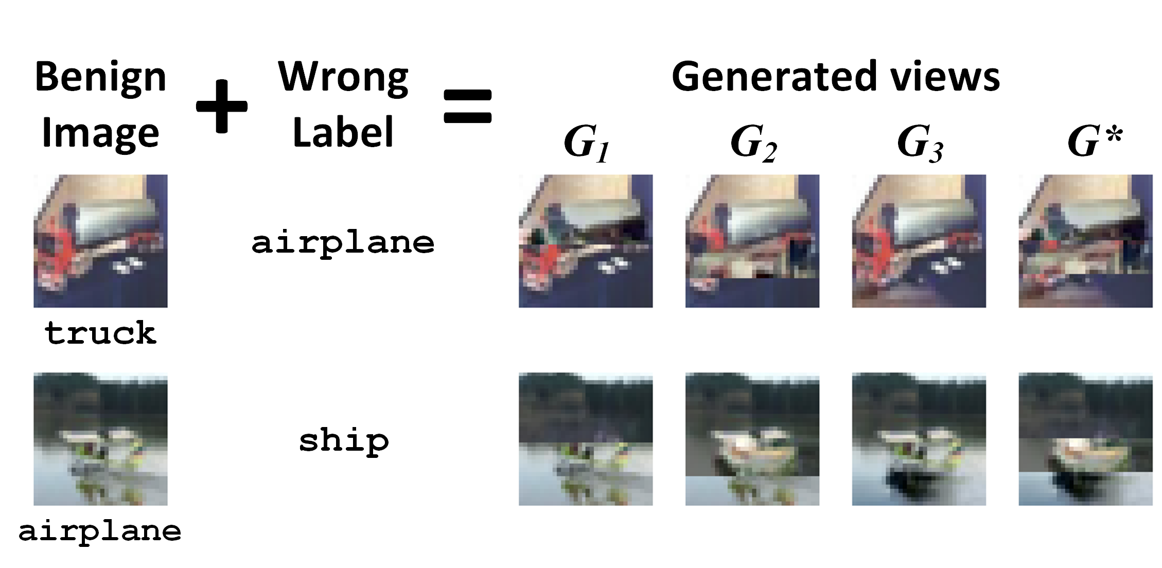
Figure 5. Misclassified benign samples (CIFAR): (1) truck image misclassified as airplane; (2) airplane image misclassified as ship. Argos is able to detect (2) as misclassified.

Finally, we reiterate that the essential objectives of the adversarial attacks are (1) to add minimum perturbation to $x$ so that it still looks like its original label $y$, and (2) to trick the classifier to label the image as a significantly different label $y^{\prime}$. Both objectives work in the favor of Argos. As shown in Table 5, Argos is significantly more effective in detecting adversarially misclassified samples.

Limitations. Argos does not perform well when the visual content of the source class $y$ and the misclassified class $y^{\prime}$ are not too distinct to each other, such that even a conventional classifier struggles to differentiate between the two classes of benign samples. For instance, a long-hair cat might look visually similar to a dog when observed from a particular angle. When the attacker uses such a cat image to force a “dog” label, Argos is less likely to detect the attack. However, for security-critical applications, where miss-classification even for benign samples is undesirable, different classes are usually quite distinct like traffic signboards. Thus, we expect Argos will perform well in security-critical applications.

Last, as shown in Table 2, it is also evident that Argos’ performance is relative to the complexity of the dataset. For a dataset whose benign classification accuracy is high, such as GTSRB and CIFAR10, Argos’ detection AUC score is consistently higher than $90\%$. Meanwhile, for a complex dataset, such as R-ImageNet, whose classification accuracy is approximately $74\%$, the Argos guarantees AUC score above $70\%$ ($>80\%$ against most attacks), which is acceptable given that the misclassification rate of the benign classifier is already high. We argue that the problem of adversarial examples usually arises in scenarios where misclassified examples can significantly damage the system integrity, i.e., when the natural classification rates with benign samples are much higher.

Detection Performance for larger Images. In the literature of adversarial example detection, it is standard practice to do proof of concept with several popular image datasets, such as MNIST, F-MNIST, GTSRB, CIFAR, Tiny-ImageNet. To perform a fair comparison with the literature, especially I-Defender (Zheng and Hong, 2018), and PixelDefend (Song et al., 2018), we used the same experimental setup that employs small images (i.e., 32$\times$32) in evaluation. Moreover, we would like to ask how Argos would perform for larger images. Hence, we further evaluate Argos with 64$\times$64 images from the Restricted-ImageNet dataset. The classification accuracy and pixel-cnn’s natural log-likelihood (NLL) achieved for this dataset are 79% and 3.97 respectively, both of which are slightly improved over 32$\times$32 images (74% classification accuracy and 4.60 NLL, as reported in Table 1). Comparing with experiment results on smaller images, the detection performance of Argos has improved for iterative attacks, such as PGD, MIM and WB, as shown in Table 6. However, for optimization based attacks like CW and single step FGSM, the performance decreased, which might be because adversary has more area to add adversarial perturbation. Nonetheless, the experiment results demonstrate that Argos is still effective against all attacks for larger images.

Table 6. Comparison of Argos performance with 64$\times$64 and 32$\times$32 images from R-ImageNet. Attack Detection Rate (ADR) evaluated with TNR=95%.

Attack	64$\times$64 images		32$\times$32 images
	ADR	AUROC	ADR	AUROC
deepFool	33	79	42	87
CW	37	76	70	91
PGD-4	86	94	42	79
PGD-8	99	99	64	87
PGD-16	99	99	84	95
MIM-4	84	93	51	79
MIM-8	99	99	71	88
MIM-16	99	99	72	89
FGSM-4	38	73	48	79
FGSM-8	50	81	75	92
FGSM-16	57	85	89	96
WB	70	86	45	71

7. Related Work

In the evasion attacks against deep neural networks, carefully crafted adversarial samples are generated to trick a deep learning model to misclassify an image/object into an incorrect class, e.g., (Rezaei and Liu, 2019; Wu and Zhu, 2020; Biggio et al., 2013; Papernot et al., 2016; Carlini and Wagner, 2017b; Xiao et al., 2018). Research has also shown that adversarial examples might fool time-limited humans (Elsayed et al., 2018). Several adversarial detectors (Hendrycks and Gimpel, 2017; Metzen et al., 2017; Samangouei et al., 2018) have been proposed to defend against adversarial attacks. These methods also reveal some unique detection challenges (Carlini and Wagner, 2017a) e.g., the introduction of perceptually small perturbations and white-box attacks. Here, we briefly review the adversarial sample detection approaches in the literature to shed light on the design of effective and generalizable detectors.

Separate Classifier Or Statistical Tests. The earlier approaches to detect adversarial examples used a separately-trained classifier  (Metzen et al., 2017; Grosse et al., 2017; Gong et al., 2017) or statistical properties  (Hendrycks and Gimpel, 2017; Feinman et al., 2017; Grosse et al., 2017). However, many of these approaches were subsequently shown to be weak (Carlini and Wagner, 2017a; Athalye et al., 2018). The most recent work in detecting adversarial examples based on statistical tests (Roth et al., 2019) achieved a 99% true positive rate (TPR) on CIFAR-10 (Krizhevsky, [n.d.]) but it was fully bypassed by later work (Hosseini et al., 2019), which decreased the TPR to less than 2%. The major limitation of these approaches is that their detections are all based on identifying anomalies in sample distributions. This makes the approach vulnerable to unknown/white-box adversaries, whose adversarial samples behave like in-distribution samples.

Generative Models. The generative models have been used in adversarial image detection, e.g., (Lee et al., 2018; Zheng and Hong, 2018; Song et al., 2018; Samangouei et al., 2018). In Argos, the generative models are used in a completely different manner than the literature. Other approaches rely on likelihood density estimation through generative model, to differentiate adversarial samples from benign. On the contrary, Argos utilizes sample generation from generative model. Performance comparison between Argos and SOTA generative-model-based adversarial detectors are reported in Section 5, while detailed analysis of the performance differences are presented in Section 5.4.

Comparison with Training Samples. Recent approaches that are proven to be successful against white-box attacks involve the comparison of test samples with all training samples (Cohen et al., 2020; Wu et al., 2021). Their major weakness is that they do not scale well with large datasets due to excessive memory and computational requirements.

Image Generation. Most similar to Argos is a recently proposed image-generation-based approach (Qin et al., 2020). The major difference between Argos and (Qin et al., 2020) is that they reconstruct the input from a high-level representation generated from a capsule classification model. But the same reconstruction technique does not give a similar performance for other classification models. Argos, on the other hand, uses an auto-regressive generation scheme that in our knowledge has never been explored in adversarial image detection before. Moreover, we use a novel multi-view approach to amplify and identify the image-label discrepancies that exist in all successful adversarial sample attack. As a result, Argos is not dependent on a classification or attack model, which makes it generally applicable.

8. Conclusion

In this paper, we present an adversarial image detector named Argos. We have observed that an adversarial instance, regardless of the attack method or the level of perturbation, always contains two inherently contradictory “souls”: the visually unchanged content and the invisible perturbation, which correspond to the true and adversarial labels, respectively. We employ a generative model to construct views to amplify the inherent discrepancies, and then design an adversary detector based on multi-view inconsistencies. Through extensive experiments, we show that Argos achieves an average attack detection rate of 80.7% (at 0.95 TNR) and AUROC score of 0.934 against six representative attacks, including the low-perturbation and white-box attacks. Argos also significantly outperforms existing adversarial example detectors in both detection accuracy and robustness. Last, Argos is a stand-alone detector that does not utilize any prior knowledge on the attacks or makes any assumption about the attack method. It could be easily adapted to any classifier/ dataset, including the ones that are already deployed.

Appendix A Adversarial Attacks against DNN

Here we introduce the adversarial attack techniques that has been used to evaluate Argos and the SOTA defense approaches.

Fast Gradient Sign Method (FGSM). FGSM assumes the linear behavior in high-dimensional spaces is sufficient to generate adversarial inputs (Goodfellow et al., 2015). Therefore, it constructs adversarial samples by applying a first-order approximation of the loss function. That is, given a data sample $(x,y)$ and the cross-entropy loss $L(\theta;x,y)$, an adversarial sample can be generated as:

$$x^{\prime}=x+\epsilon\cdot sign(\nabla_{x}L(\theta))$$

where $\nabla_{x}L(\theta)$ is the gradient of the loss function w.r.t. $x$.

Projected Gradient Descent (PGD). As an iterative version of FGSM, PGD (Madry et al., 2018) selects the original image as a starting point and generates adversarial examples as follows. It can generate strong adversarial examples and thus is often used as a baseline attack to evaluate the defense designs. Procedurally, it starts from a benign image $x$ and iteratively modifies it into an adversarial image by

$$x^{t+1}=clip_{x+\epsilon}[x^{t}+\alpha\cdot sign(\nabla_{x}L(\theta))]$$

where $clip_{x+\epsilon}(x^{\prime})$ is to keep $x^{\prime}$ into the $\epsilon$-vicinity of $x$ and $\alpha$ can be set as $\epsilon/T$ with $T$ being the number of iterations.

Momentum Iterative attacks. Inspired by the momentum optimizer, Dong et al. (Dong et al., 2018) proposed to integrate the momentum memory into the iterative process and derived a new iterative algorithm, called momentum iterative FGSM (MI-FGSM). Specifically, MI-FGSM updates the adversarial samples iteratively as follows.

$$x^{0} =x$$

$$x^{t+1} =clip_{x+\epsilon}[x^{t}+\alpha\cdot sign(g^{t+1})]$$

where $g^{t+1}=g^{t}+\nabla L(\theta;x^{\prime},y)/\left\|\nabla L(\theta;x^{\prime},y)\right\|_{1}$.

DeepFool. DeepFool (Moosavi-Dezfooli et al., 2016) computes the minimal adversarial perturbation for an image based on an iterative linearization of the classifier. In particular, given a linear binary classifier, the minimal perturbation to change the classifier’s decision for an input $x_{0}$ corresponds to the orthogonal projection of $x_{0}$ on $\mathscr{F}$, where $\mathscr{F}$ is the hyperplane at zero of $F$ (i.e., $\mathscr{F}=\{x:F(x)=0\}$). At each iteration $i$, the algorithm linearizes $F$ around the current point $x_{i}$ and computes the minimal perturbation of the classifier as:

$$\underset{r_{i}}{arg\,min}\left\|r_{i}\right\|_{2}\;\;\;\;subject\,to\;\;\;\;F(x_{i})+\nabla F(x_{i})^{T}r_{i}=0$$

where $r_{i}$ estimates the robustness of $F$ at $x_{i}$ and is computed as:

$$r_{*}(x_{i})=-\frac{F(x_{i})}{\left\|\nabla F(x_{i})\right\|_{2}^{2}}\nabla F(x_{i})$$

The iteration stops when the sign of the classifier is changed.

The Carlini & Wagner (C&W) Attack. The C&W attacks (Carlini and Wagner, 2017b) are considered as optimization-based strong white-box attacks. Since, in our threat model we considered classifier Model $F(.)$ will be known for all type attacks, we can use C&W to attack $F(.)$. In this method, the aim is to find the small perturbation $\delta$ satisfying:

$$\underset{\delta}{arg\,min}\left\|\delta\right\|_{p}\;\;\;subject\,to\;\;\;\;F(x+\delta)=t,\ x+\delta\in[0,255]^{n}$$

where $t$ is the target label. To solve the optimization problem, an objective function $f$ is selected such that when $f(x+\delta)\leq 0$, $F(x+\delta)=t$. (Carlini and Wagner, 2017b) adopted the below objective function and generated adversarial samples with the $L_{0},L_{2}$, and $L_{\infty}$ distance metrics.

$$f(x^{\prime})=max(max\{Z(x^{\prime})_{i}:i\neq t\}-Z(x^{\prime})_{t},-k)$$

where $Z$ is the logits function and $k$ is used to control the confidence of the misclassification.