capbtabboxtable[][\FBwidth]
11institutetext: SIRIUS, Department of Information, University of Oslo, Norway
11email: jieyingc@ifi.uio.no
22institutetext: LISN, Univ. Paris-Sud, CNRS, Université Paris-Saclay, Orsay, France
22email: {ma, yang}@lri.fr
33institutetext: University of Milano-Bicocca, Milan, Italy
33email: rafael.penaloza@unimib.it
Union and Intersection of all Justifications
Abstract
We present new algorithms for computing the union and intersection of all justifications for a given ontological consequence without first computing the set of all justifications. Through an empirical evaluation, we show that our approach works well in practice for expressive description logics. In particular, the union of all justifications can be computed much faster than with existing justification-enumeration approaches. We further discuss how to use these results to repair ontologies.
1 Introduction
A justification for a consequence refers to a minimal subset of the ontology, which still entails . The problem of computing justifications, also known as axiom pinpointing, has been widely studied in the context of description logics [27]. Axiom pinpointing methods can be separated into two main classes, commonly known as black-box and glass-box.
Black-box approaches [18, 19, 26] use existing reasoners as an oracle, and require no further modification of the reasoning method. Therefore, these approaches work for ontologies written in any monotonic logical language (including expressive DLs such as ), as long as a reasoner supporting it exists. In their most naïve form, black-box methods check all possible subsets of the ontology for the desired entailment and compute the justifications from these results. In reality, many optimisations have been developed to reduce the number of calls needed, and avoid irrelevant work.
Glass-box approaches, on the other hand, modify the reasoning algorithm to output one or all justifications directly, from only one call. While the theory for developing glass-box methods has been developed for tableaux and automata-based reasoners [6, 5, 4, 7], in practice not many of these methods have been implemented, as they require new implementation efforts and deactivating the optimisation techniques that make reasoners practical. A promising approach, first proposed in [32] is to reduce, through a reasoning simulation, the axiom pinpointing problem to an enumeration problem from a propositional formula, and use state-of-the-art SAT-solving methods to enumerate all the justifications. This idea has led to effective axiom pinpointing systems developed primarily for the lightweight DL [20, 1, 2, 3, 24].
The interest of axiom pinpointing goes beyond enumerating justifications. Modelling ontologies is a time-consuming and fallible task. Indeed, during the modelling phase it is not uncommon to discover unexpected or wrong entailments. One way to fix these errors is to diagnose the causes by computing a hitting set of all the justifications. However, as there might exist exponential many justifications for a given entailment w.r.t. an ontology, even for -ontologies, finding all justifications is not feasible in general. One approach is to approximate the information by the union and intersection of all justifications. If the intersection is not empty, then any axiom in this intersection, when removed, guarantees that the consequence will not follow anymore. From the union, a knowledge engineer has a more precise view on the problematic instances, and can make a detailed analysis.
Although much work has focused on methods for computing one or all justifications efficiently, to the best of our knowledge there is little work on computing their intersection or union without enumerating them first, beyond the approximations presented in [29, 28]. In this paper, we propose an algorithm of computing the intersection of all justifications. This algorithm has the same worst-case behaviour as the black-box algorithm of computing one justification. Additionally, we present two approaches of computing the union of all justifications, one is based on the black-box algorithm of finding all justifications and the other approach uses the SAT-tool cmMUS.
The paper is structured as follows. In Section 2 we recall relevant definitions of description logics and propositional logic. Section 3 presents the algorithm for computing the intersection of all justifications without computing any single justification. We propose two methods of computing the union of all justifications in Section 4. We explain how to use the union and intersection of all justifications to repair ontologies in Section 5. Before concluding, an evaluation of our methods on real-world ontologies is presented in Section 6.
2 Justifications and Repairs in
We briefly recall the notions of justifications and repairs in . Let , and be mutually disjoint sets of concept names, role names, and individual names. The set of -concepts is built through the following grammar rule
where and . An -TBox is a finite set of general concept inclusions (GCIs) of the form and role inclusions , where and are -concepts and . An ABox is a finite set of concept assertions of the form and role assertions , where , and . An ontology consists of an TBox and an ABox.
The semantics of this logic is defined in terms of interpretations. An interpretation is a pair where is a non-empty set called the domain, and is the interpretation function, which maps each concept name to a subset , each role name to a binary relation and each individual to a domain element . The interpretation function is extended to -concepts as usual: , , , , , , and . The interpretation satisfies iff and it satisfies iff . We write if satisfies the axiom . The interpretation is a model of an ontology if satisfies all axioms in . An axiom is entailed by , denoted as , if for all models of . We use to denote the size of , i.e., the number of axioms in .
For this paper, we are interested in the notions of justification and repair.
Definition 1 (Justification, repair)
Let be an ontology and a GCI. A justification for is a subset such that and for any , . denotes the set of all justifications of w.r.t. . A repair for is a subontology such that , but for any . We denote the set of all repairs as .
Briefly, a justification is a minimal subset of an ontology that preserves the conclusion. Dually, a repair is a maximal sub-ontology that does not preserve the consequence.
Now we consider a propositional language with a finite set of propositional variables . A literal is a variable or its negation . A clause is a disjunction of literals, denoted by [10]. A Boolean formula in Conjunctive Normal Form (CNF) is a conjunction of clauses. A CNF formula is satisfiable iff there exists a truth assignment such that satisfies all clauses in . We can also consider a CNF formula as a set of clauses. A subformula is a Minimally Unsatisfiable Subformula (MUS) iff is unsatisfiable, but for every is satisfiable.
3 Computing the Intersection of all Justifications
We first study the problem of computing the intersection of all justifications, which we often call the core. Algorithm 1 provides a method for finding this core.
The algorithm is inspired by the known black-box approach for finding justifications [17, 7]. Starting from a justification-preserving module (in this case, the locality-based module, Line 3), we try to remove one axiom (Line 4). If the removal of the axiom removes the entailment (Line 5), then must belong to all justifications ( is a sine qua non requirement for entailment within ), and is thus added to the core (Line 6).
Algorithm 2, on the other hand, generalises the known algorithm for computing a single justification, by considering a (fixed) set that is known to be contained in all justifications. If , the approach works as usual; otherwise, the algorithm avoids trying to remove any axiom from . This reduces the number of calls to the black-box reasoner, potentially decreasing the overall execution time.
As mentioned already, the choice for a locality-based module in these algorithms is arbitrary, and any justification-preserving module would suffice. In particular, we could compute lean kernel [29, 21] for -ontologies, and minimal subsumption modules [11, conf/gcai/ChenL018] for -ontologies instead, which is typically smaller thus reducing the number of iterations within the algorithms. However, as it could be quite expensive to compute such modules, it might not be worthwhile in some cases. The following theorem shows that Algorithm 1 correctly computes the intersection of all justifications.
Theorem 3.1
Let be an ontology and a GCI. Algorithm 1 computes the intersection of all justifications of w.r.t. .
Algorithm 1, like all black-box methods for computing justifications, calls a standard reasoner times. In terms of computational complexity, computing the core requires as many computational resources as computing a single justification. However, computing one justification might be faster in practice, as the size of decreases throughout the execution of Algorithm 2. Clearly, if the core coincides with one justification , then is the only justification.
Corollary 1
Let be an ontology, a GCI; and let be the core and a justification for . If , is the only justification for .
4 Computing the Union of all Justifications
We now present two algorithms of computing the union of all justifications. The first algorithm follows a black-box approach that calls a standard reasoner as oracle using the core of justifications. This is inspired by Reiter’s Hitting Set Tree algorithm [30] and partially in line with [17, 34]. For the second algorithm, we reduce the problem of computing the union of all justifications to the problem of computing the union of MUSes of a propositional formula. Note that the second algorithm works only for -ontologies, while the first algorithm can be applied to ontologies with any expressivity, as long as a reasoner is available.
4.1 Black-box algorithm
The black-box algorithm of computing all justifications [34] was inspired by the algorithm of computing all minimal hitting sets [30]. Some of the improvements to prune the search space were already proposed in [30]. Our method for computing the union of all justifications (Algorithm 3) works in a similar manner, but with a few key differences.
To avoid computing all justifications, we prune the search space when all remaining justifications are fully contained in the union computed so far (Lines 11-12). In addition, we use the core to speed the search. As the axioms in the core must appear in every justification, we can reduce the number of calls made to the reasoner, and optimise the single justification computation (Line 17). Finally, when we organise our search space, we do not need to consider the axioms in the core (Line 22).
We now describe the Union-of-All-Justifications procedure in detail. Given an ontology , a signature , and the intersection of all justifications of w.r.t. as input, a syntactic -locality module of w.r.t. is extracted from (Lines 2). The justification search tree is a four-tuple , where is a finite set of nodes, is a set of edges, is an edge labelling function, mapping every edge to an axiom , and is the root node. We initialise the variable to represent a justification search tree for having only root node . Besides, the variables , containing the justifications that have been computed so far, and , containing the already explored nodes of , are both initialised with the empty set. The queue of nodes in that still has to be explored is also set to contain the node as its only element.
The algorithm then enters a loop (Lines 4–24) that runs while is not empty. The loop extracts the first element from and adds it to (Line 5). The axioms that label the edges of the path from to in are collected in the set (Line 7). After that, the algorithm checks whether is redundant. The detailed method for checking redundancy is described in Algorithm 4. The path is redundant iff there exists an explored node such that (a) the axioms in are exactly the axioms labelling the edges of the path from to in (Lines 4–6), or (b) is a leaf node of and the edges of are only labelled with axioms from (Lines 7–8). Case (a) corresponds to early path termination in [30, 17]: the existence of implies that all possible extensions of have already been considered. Case (b) implies that the axioms labelling the edges of lead to the fact that can not be entailed be the remaining TBox when removed from . Therefore, by monotonicity of , we infer that removing from also has the same consequence implying that we do not need to explore and all its extensions.
The current iteration can be terminated immediately if (Lines 9–10) as no subset of can be a justification of w.r.t. . In contrast to other black-box algorithms for computing justifications, we additionally check whether is a subset of . If so, no new axioms belonging to the union of all justifications appear in this sub-tree. Hence, the algorithm does not need to explore it any further. Subsequently, the variable that will hold a justification of is initialised with . At this point we can check if a justification has already been computed for which (Lines 14–15) holds, in which casewe set to . This optimisation step can also be found in [30, 17] and it allows us to avoid a costly call to the Single-Justification procedure. Otherwise, in Line 17 we call Single-Justification on to obtain a justification of w.r.t. . We then check whether is equal to (Lines 18–19), in which case the search for additional justifications can be terminated (recall Corollary 1). Otherwise, the justification is added to in Line 20 and the union of all justifications is updated in Line 21. Finally, for every , the algorithm extends the tree in Lines 22–24 by adding a child to , connected by an edge labelled with . Note that it is sufficient to take as a set with cannot be a justification of w.r.t. . The procedure finishes by returning the set .
Note that this algorithm only adds justifications to . For completeness, one can show that the locality-based module of w.r.t. contains all the minimal modules of w.r.t. . Moreover, it is easy to see that the proposed optimisations do not lead to a minimal module not being computed. Overall, we obtain the following result.
Theorem 4.1
Let be an ontology, a GCI, and the core of w.r.t. . The procedure Union-of-All-Justifications computes the union of all justifications of w.r.t. .
Algorithm 3 terminates on any input as the paths in the module search tree for that is constructed during the execution represent all the permutations of the axioms in that are relevant for finding all minimal modules. It is easy to see that the procedure Union-of-All-Justifications runs in exponential time in size of (and polynomially in , , and ) in the worst case.
4.2 MUS Membership Problem
We now show how to compute the union of all justifications of a GCI by a membership approach. The idea is to check the membership of each axiom, i.e., whether it is a member of some justification. The main procedure is: firstly, as a pre-processing step, we compute a CNF formula using the consequence-based reasoner condor111We restrict to in this section as condor only accepts -TBoxes. proposed in [9]. Then, we compute the union of all justifications of by checking the membership for each axiom using the SAT-tool cmMUS [16] and . In generally, the classification of an -TBox is of exponential complexity. Since the MUS-membership problem is -complete [22], it follows that this method runs in exponential time.
Specifically, the method is divided in two steps:
-
1.
Compute CNF formula . Let denote (possibly empty) conjunctions of concepts, and (possibly empty) disjunctions of concepts; condor classifies the TBox through the inference rules in Table 1.
Table 1: Inference rules of condor -
2.
Check membership of each axiom using cmMUS. Given an CNF formula and a subformula , the algorithm cmMUS is used to determine whether there is a MUS such that . We say if there exists such MUS and otherwise. The membership is checked as follows:
-
(a)
Define a CNF-formula , where each literal corresponds to an axiom , and , where is the given conclusion.
-
(b)
Define . Then is unsatisfiable; each MUS corresponds to a justification of ; and , iff belongs to some justifications of .
-
(a)
Note that only a small number of clauses in are related to the derivation of . In practice, (i) is the subformula contributing to the derivation of obtained by tracing back from , (ii) is the subformula including only that appears in . Using instead of as the input of algorithm cmMUS can significantly accelerate the cmMUS algorithm.
5 Repairing Ontologies
In this section we propose a notion of optimal repair and provide a method for computing all such optimal repairs.
Definition 2 (Optimal Repair)
Let be an ontology, a GCI, and the set of all repairs for . We say is an optimal repair for , if holds for every .
That is, an optimal repair is a repair such that removes the least amount of axioms from the original ontology. It is also important to recall the notion of a hitting set
Definition 3 (HS)
We say is a minimal hitting set for a sets if for every .
We say is the smallest minimal hitting set if is the smallest among all minimal hitting set. The following proposition shows how we can compute the set of all optimal repairs through a hitting set computation [31, 23, 6].
Proposition 1
Let be the set of all justifications for the GCI w.r.t. the ontology . If is the set of all smallest minimal hitting sets for , then is the set of all optimal repairs for .
When the core is not empty, a set that consists of only one axiom from the intersection of all justifications is a smallest hitting set for all justifications. We get the following corollary, stating how to compute all optimal repairs faster in this case, as a simple consequence of Proposition 1.
Corollary 2
Let be an ontology, a GCI and the core for . If , then is the set of all optimal repairs for .
The application of the union of all justifications can be used as a step towards deducing IAR entailments [28].
6 Evaluation
To evaluate the performance of our algorithms in real-world ontologies, we built a prototypical implementation. The black-box algorithm is implemented in Java and uses the OWL API [15] to access ontologies and HermiT [14] as a standard reasoner. The MUS-membership algorithm (MUS-MEM) is implemented in Python and calls cmMUS [16] to detect whether a clause is a member of MUSes. The ontologies used in the evaluation come from the classification task at the ORE competition 2014 [25]. Among them, we selected the ontologies that have less than 10,000 axioms, for a total of 95 ontologies. In the experiments, we computed a single justification, the intersection and union of all justifications for all atomic concept inclusions that are entailed by the ontologies.222An atomic concept inclusion is the inclusion that in the form of , where and are concept names. All experiments ran on two processors Intel® Xeon® E5-2609v2 2.5GHz, 8 cores, 64Go, Ubuntu 18.04. All the figures in this section plot the logarithmic computation time (in the vertical axis) of each test instance (in the horizontal axis).
| min | 0.001s | 0.001s |
|---|---|---|
| max | 226.608s | 341.560s |
| mean | 0.400s | 0.456s |
| median | 0.009s | 0.002s |
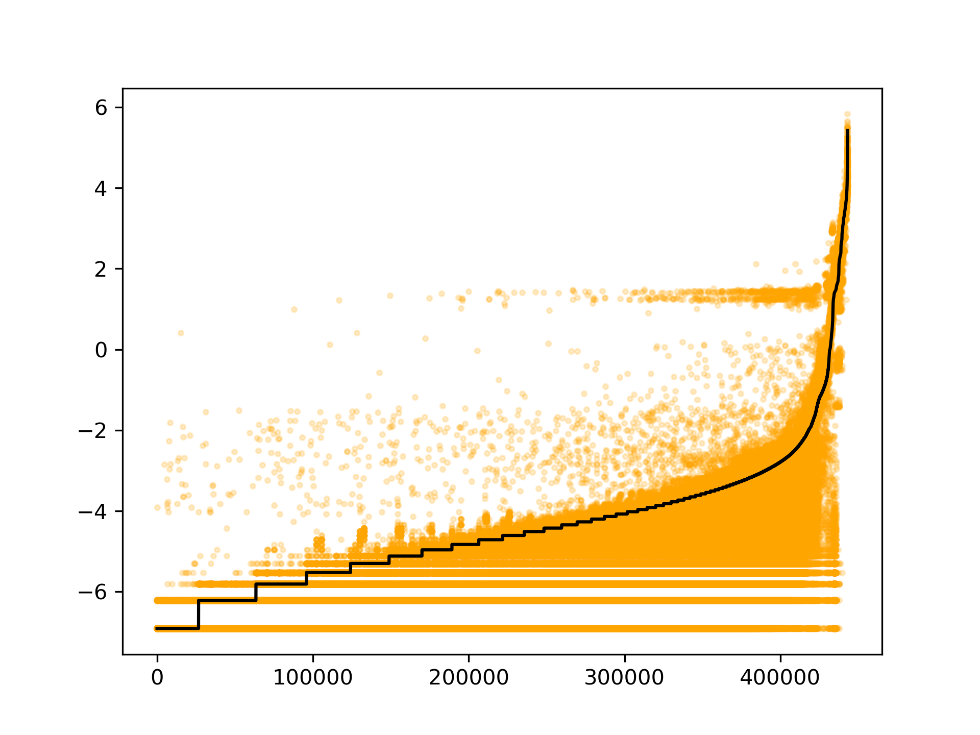
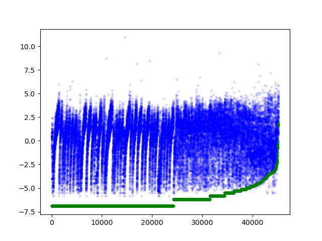
Computation time of the core vs. a single justification.
Fig. 2 compares the time to compute the core against computing a single justification. The instances in the horizontal axis are ordered according to the single-justification computation time, represented by the black line. Orange dots represent the core computation time through Algorithm 1. Table 2 provides some basic statistics for comparison. Generally, computing the core is almost as fast as computing one justification as expected. Note that, in terms of computational complexity computing the core and one justification are equally hard problems, the size of the remaining ontology reduces during the latter process. Intuitively, if , checking whether a subsumption is satisfied by would be faster than checking it on .
Computation time of the union of all justifications.
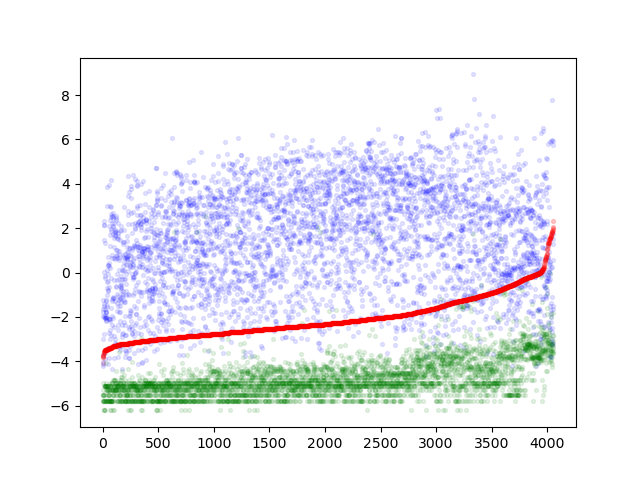
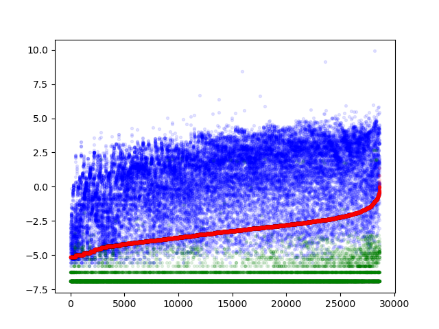
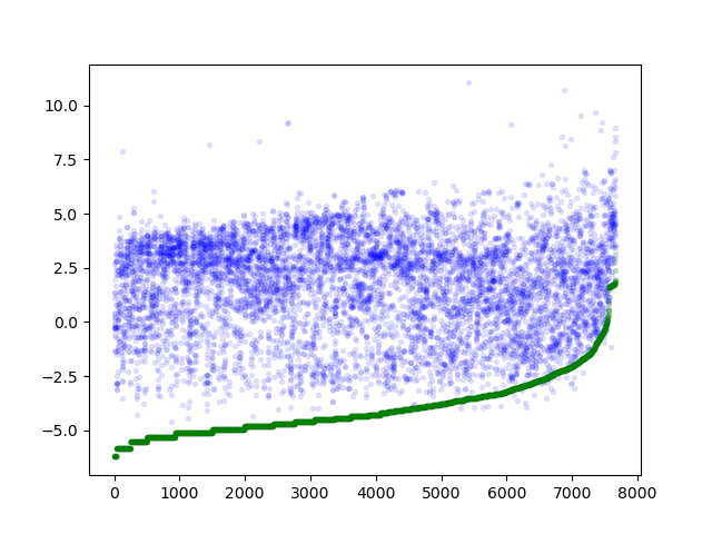
As a benchmark, we use OWL API to compute all justifications and then get the union. As our second algorithm could compute the union of all justifications only for -ontologies, we separate our ontologies into two categories: one is -ontologies and the other one is the ontologies that are more expressive than . The computation time for the union of all justifications for -ontologies is shown in Fig. 6 (the cases with several justifications) and Fig. 6 (the cases with only one justification). Figs. 6 and 6 show the computation time of the union of all justifications for more expressive ontologies when there exists multiple justifications and only one justification respectively. In Figs. 6–6, each blue, green or red dot corresponds to computation time of the union by OWL API, the black-box algorithm or the MUS-MEM algorithm for a conclusion respectively. We order the conclusions along the X-axis by increasing order of computation time of MUS-MEM algorithms in Figs. 6 and Fig. 6, and by the black-box performance in the latter two figures. We observe from these plots that the black-box algorithm outperforms other methods, and when available, MUS-MEM tends to perform better than a direct use of the OWL API.
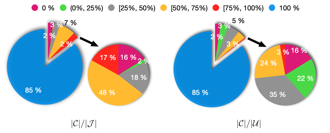
Size comparisons for justifications, cores, and unions of justifications.
Fig. 7 illustrates the ratio of the size of the core to the size of a random justification and to the size of the union of all justifications. In our experiments, the intersection of all justifications for only 2.35% subsumptions is empty, which means that we could use Corollary 2 to compute optimal repairs for 97.65% of the cases. Moreover, for more than 85% cases, the size of a justification () equals to the size of the core (), which indicates that there exists only one justification. When several justifications exist (the second chart from the left of Fig. 7), the ratio of to a random falls between 50% to 75% for almost half of the cases. The right-most chart displays the distribution of the ratio of to the union of all justifications when there exist multiple justifications. The ratio distributes quite evenly between 0% (not including) to 75%. Interestingly, the intersection of all justifications is empty for only 16% subsumptions even when several justifications exist.
7 Conclusions
In this paper, we presented algorithms for computing the core (that is, the intersection of all justifications) and the union of all justifications for a given DL consequence. Most of the algorithms are based on repeated calls to a (black-box) reasoner, and hence apply for ontologies and consequences of any expressivity, as long as a reasoner exists. The only exception is a MUS-based approach for computing the union of all justifications, which depends on the properties of the consequence-based method implemented by condor. Still, the approach should be generalisable without major problems to any language for which consequence-based reasoning methods exists like, for instance, [13, 12].
As an application of our work, we study how to find optimal repairs effectively, through the information provided by the core and the union of all justifications. Through an empirical analysis, run over more than 100,000 consequences from almost a hundred ontologies from the ORE 2014 competition we observe that our methods behave better in practice than the usual approach through the OWL API. A more detailed analysis of the experimental results is left for future work.
Our experiments also confirm an observation that has already been made for light-weight ontologies [33], and to a smaller degree in the ontologies from the BioPortal corpus [8]; namely, that consequences tend to have one, or only a few, overlapping justifications. In our case, we exploit this fact, and the efficient core computation algorithm to find optimal repairs in more than 97% of the test instances: those with exactly one justification, where removing any axioms from it leads to an optimal repair.
References
- [1] M. F. Arif, C. Mencía, A. Ignatiev, N. Manthey, R. Peñaloza, and J. Marques-Silva. Beacon: An efficient sat-based tool for debugging ontologies. In International Conference on Theory and Applications of Satisfiability Testing, pages 521–530. Springer, 2016.
- [2] M. F. Arif, C. Mencía, and J. Marques-Silva. Efficient axiom pinpointing with EL2MCS. In Joint German/Austrian Conference on Artificial Intelligence (Künstliche Intelligenz), pages 225–233. Springer, 2015.
- [3] M. F. Arif, C. Mencía, and J. Marques-Silva. Efficient MUS enumeration of Horn formulae with applications to axiom pinpointing. In International Conference on Theory and Applications of Satisfiability Testing, pages 324–342. Springer, 2015.
- [4] F. Baader and B. Hollunder. Embedding defaults into terminological knowledge representation formalisms. Journal of Automated Reasoning, 14(1):149–180, 1995.
- [5] F. Baader and R. Peñaloza. Automata-based axiom pinpointing. J. Autom. Reason., 45(2):91–129, 2010.
- [6] F. Baader and R. Peñaloza. Axiom pinpointing in general tableaux. J. Log. Comput., 20(1):5–34, 2010.
- [7] F. Baader, R. Peñaloza, and B. Suntisrivaraporn. Pinpointing in the description logic EL+. In J. Hertzberg, M. Beetz, and R. Englert, editors, Proceedings of the 30th Annual German Conference on AI, KI 2007, volume 4667 of Lecture Notes in Computer Science, pages 52–67. Springer, 2007.
- [8] S. P. Bail. The justificatory structure of OWL ontologies. PhD thesis, University of Manchester, UK, 2013.
- [9] A. Bate, B. Motik, B. C. Grau, D. T. Cucala, F. Simančík, and I. Horrocks. Consequence-based reasoning for description logics with disjunctions and number restrictions. J. Artif. Int. Res., 63(1):625–690, Sept. 2018.
- [10] C.-L. Chang and R. C.-T. Lee. Symbolic logic and mechanical theorem proving. Academic press, 2014.
- [11] J. Chen, M. Ludwig, Y. Ma, and D. Walther. Zooming in on ontologies: Minimal modules and best excerpts. In Proc. of ISWC’17, Part I, volume 10587 of Lecture Notes in Computer Science, pages 173–189. Springer, 2017.
- [12] D. T. Cucala, B. C. Grau, and I. Horrocks. Consequence-based reasoning for description logics with disjunction, inverse roles, number restrictions, and nominals. In J. Lang, editor, Proceedings of the Twenty-Seventh International Joint Conference on Artificial Intelligence, IJCAI 2018, pages 1970–1976. ijcai.org, 2018.
- [13] D. T. Cucala, B. C. Grau, and I. Horrocks. Sequoia: A consequence based reasoner for SROIQ. In M. Simkus and G. E. Weddell, editors, Proceedings of the 32nd International Workshop on Description Logics, volume 2373 of CEUR Workshop Proceedings. CEUR-WS.org, 2019.
- [14] B. Glimm, I. Horrocks, B. Motik, G. Stoilos, and Z. Wang. HermiT: an OWL 2 reasoner. Journal of Automated Reasoning, 53(3):245–269, 2014.
- [15] M. Horridge and S. Bechhofer. The OWL API: A Java API for OWL ontologies. Semantic Web, 2(1):11–21, 2011.
- [16] M. Janota and J. Marques-Silva. cmMUS: A tool for circumscription-based mus membership testing. In International Conference on Logic Programming and Nonmonotonic Reasoning, pages 266–271. Springer, 2011.
- [17] A. Kalyanpur, B. Parsia, M. Horridge, and E. Sirin. Finding all justifications of OWL DL entailments. In Proceedings of ISWC 2007 & ASWC 2007, volume 4825 of LNCS, pages 267–280. Springer, 2007.
- [18] A. Kalyanpur, B. Parsia, E. Sirin, and J. Hendler. Debugging unsatisfiable classes in OWL ontologies. Journal of Web Semantics, 3(4):268–293, 2005.
- [19] A. A. Kalyanpur. Debugging and repair of OWL ontologies. PhD thesis, 2006.
- [20] Y. Kazakov and P. Skočovskỳ. Enumerating justifications using resolution. In International Joint Conference on Automated Reasoning, pages 609–626. Springer, 2018.
- [21] P. Koopmann and J. Chen. Deductive module extraction for expressive description logics. In C. Bessiere, editor, Proceedings of IJCAI’20, pages 1636–1643. ijcai.org, 2020.
- [22] P. Liberatore. Redundancy in logic i: Cnf propositional formulae. Artificial Intelligence, 163(2):203–232, 2005.
- [23] M. H. Liffiton and K. A. Sakallah. On finding all minimally unsatisfiable subformulas. In F. Bacchus and T. Walsh, editors, Proceedings of the 8th International Conference on Theory and Applications of Satisfiability Testing (SAT 2005), volume 3569 of Lecture Notes in Computer Science, pages 173–186. Springer, 2005.
- [24] N. Manthey, R. Peñaloza, and S. Rudolph. Efficient axiom pinpointing in EL using sat technology. In Description Logics, 2016.
- [25] B. Parsia, N. Matentzoglu, R. S. Gonçalves, B. Glimm, and A. Steigmiller. The OWL reasoner evaluation (ORE) 2015 competition report. Journal of Automated Reasoning, pages 1–28, 2015.
- [26] B. Parsia, E. Sirin, and A. Kalyanpur. Debugging owl ontologies. In Proceedings of the 14th international conference on World Wide Web, pages 633–640, 2005.
- [27] R. Peñaloza. Axiom pinpointing. In G. Cota, M. Daquino, and G. L. Pozzato, editors, Applications and Practices in Ontology Design, Extraction, and Reasoning, volume 49 of Studies on the Semantic Web, pages 162–177. IOS Press, 2020.
- [28] R. Peñaloza. Error-tolerance and error management in lightweight description logics. Künstliche Intell., 34(4):491–500, 2020.
- [29] R. Peñaloza, C. Mencía, A. Ignatiev, and J. Marques-Silva. Lean kernels in description logics. In E. Blomqvist, D. Maynard, A. Gangemi, R. Hoekstra, P. Hitzler, and O. Hartig, editors, Proceeding of ESWC’17, volume 10249 of Lecture Notes in Computer Science, pages 518–533, 2017.
- [30] R. Reiter. A theory of diagnosis from first principles. Artificial Intelligence, 32(1):57–95, 1987.
- [31] S. Schlobach and R. Cornet. Non-standard reasoning services for the debugging of description logic terminologies. In G. Gottlob and T. Walsh, editors, Proceedings of the Eighteenth International Joint Conference on Artificial Intelligence, pages 355–362. Morgan Kaufmann, 2003.
- [32] R. Sebastiani and M. Vescovi. Axiom pinpointing in lightweight description logics via Horn-SAT encoding and conflict analysis. In R. A. Schmidt, editor, Proceedings of the 22nd International Conference on Automated Deduction, volume 5663 of Lecture Notes in Computer Science, pages 84–99. Springer, 2009.
- [33] B. Suntisrivaraporn. Polynomial time reasoning support for design and maintenance of large-scale biomedical ontologies. PhD thesis, Dresden University of Technology, Germany, 2009.
- [34] B. Suntisrivaraporn, G. Qi, Q. Ji, and P. Haase. A modularization-based approach to finding all justifications for OWL DL entailments. In J. Domingue and C. Anutariya, editors, The Semantic Web, pages 1–15, Berlin, Heidelberg, 2008. Springer Berlin Heidelberg.