Covariant formulation of refracted gravity

We propose a covariant formulation of refracted gravity (RG), which is a classical theory of gravity based on the introduction of gravitational permittivity — a monotonic function of the local mass density — in the standard Poisson equation. Gravitational permittivity mimics dark matter phenomenology. The covariant formulation of RG (CRG) that we propose belongs to the class of scalar-tensor theories, where the scalar field $\varphi$ has a self-interaction potential $\mathcal{V}(\varphi)=-\Xi\varphi$, with $\Xi$ being a normalization constant. We show that the scalar field is twice the gravitational permittivity in the weak-field limit. Far from a spherical source of density $\rho_{\mathrm{s}}(r)$, the transition between the Newtonian and the RG regime appears below the acceleration scale $a_{\Xi}=(2\Xi-8\pi G\rho/\varphi)^{1/2}$, with $\rho=\rho_{\mathrm{s}}+\rho_{\mathrm{bg}}$ and $\rho_{\mathrm{bg}}$ being an isotropic and homogeneous background. In the limit $2\Xi\gg 8\pi G\rho/\varphi$, we obtain $a_{\Xi}\sim 10^{-10}$ m s^-2. This acceleration is comparable to the acceleration $a_{0}$ originally introduced in MOdified Newtonian Dynamics (MOND). From CRG, we also derived the modified Friedmann equations for an expanding, homogeneous, and isotropic universe. We find that the same scalar field $\varphi$ that mimics dark matter also drives the accelerated expansion of the Universe. From the stress-energy tensor of $\varphi$, we derived the equation of state of a redshift-dependent effective dark energy $w_{\mathrm{DE}}=p_{\mathrm{DE}}/\rho_{\mathrm{DE}}$. Current observational constraints on $w_{\mathrm{DE}}$ and distance modulus data of type Ia supernovae suggest that $\Xi$ has a comparable value to the cosmological constant $\Lambda$ in the standard model. Since $\Xi$ also plays the same role of $\Lambda$, CRG suggests a natural explanation of the known relation $a_{0}\sim\Lambda^{1/2}$. CRG thus appears to describe both the dynamics of cosmic structure and the expanding Universe with a single scalar field, and it falls within the family of models that unify the two dark sectors, highlighting a possible deep connection between phenomena currently attributed to dark matter and dark energy separately.

1 Introduction

The current standard $\Lambda$ cold dark matter ($\Lambda$CDM) cosmological model assumes that gravitational interactions are ruled by general relativity (GR); the model relies on the existence of collisionless non-baryonic CDM, and a positive cosmological constant $\Lambda$ (Ostriker & Steinhardt 1995). Non-baryonic dark matter is required to account for the abundance of light elements (Cyburt et al. 2016), the amplitude of the power spectrum of the temperature anisotropies in the cosmic microwave background (CMB) (Aghanim et al. 2020b), and the dynamics of cosmic structures (Clowe et al. 2006; Dodelson et al. 2001; Del Popolo 2014; Akrami et al. 2020; Aghanim et al. 2020a). The cosmological density parameter $\Omega_{\Lambda 0}=\Lambda/3H_{0}^{2}$ associated with $\Lambda$, with $H_{0}$ being the Hubble constant, accounts for the negative value of the deceleration parameter $q_{0}$ measured with the Hubble diagram of type Ia supernovae (SNeIa) (Riess et al. 1998; Perlmutter et al. 1999). The curvature of the Universe, $\Omega_{k}=\Omega_{\Lambda 0}+\Omega_{0}-1$, measured from the CMB power spectrum, suggests a null curvature (Aghanim et al. 2020c).

Although the $\Lambda$CDM model agrees with most of the rich observational information currently available, a number of tensions are present both on large cosmic scales and on the scale of galaxies. The Hubble constant $H_{0}$ estimated with the distance ladder in the local Universe (Riess et al. 2016, 2019) is more than $4\sigma$ larger than $H_{0}$ inferred from the measurements of the CMB (Verde et al. 2019). The observed abundances of the light elements are consistent with the Big Bang nucleosynthesis scenario, except ⁷Li, whose abundance is a factor of $\sim 3$ smaller (Mathews et al. 2020). Numerous features of the CMB temperature anistropies are present on large scales (Ade et al. 2016). The probability of some of these features to appear individually is $\lesssim 0.1\%$; the combined probability of the uncorrelated features is $\lesssim 0.001\%$ and might represent a serious challenge to the $\Lambda$CDM model (Schwarz et al. 2016; Luongo et al. 2022). The lensing amplitude in the CMB power spectra is enhanced compared to $\Lambda$CDM expectations (Aghanim et al. 2020b) and would suggest a positive rather than a null curvature of the Universe (Handley 2021; Di Valentino et al. 2019). A slight tension also appears for the normalization of the power spectrum $\sigma_{8}$ (e.g. Raveri 2016): the value inferred from the CMB measurements (Aghanim et al. 2020c) is $2\sigma$ larger than the value derived from the tomographic weak gravitational lensing analysis of the Kilo-Degree Survey (KiDS) imaging data (Hildebrandt et al. 2017).

In addition, the cosmological constant poses a fine-tuning problem that is theoretically challenging. If we associate $\Lambda$ with the ground state energy level of the vacuum in quantum field theory, its measured value, $\Lambda\sim 10^{-12}$ eV⁴, appears to be $\sim 120$ orders of magnitude smaller than expected (Weinberg 1989; Padilla 2015). If we associate $\Lambda$ with the energy scale up to which the standard model of particle physics has been tested, $\sim 1$ TeV, the discrepancy reduces to $\sim 60$ orders of magnitude (Joyce et al. 2015), but it remains severe. The most popular solution to the $\Lambda$ problem is to suppress $\Lambda$ in the Einstein-Hilbert action and generate the accelerated expansion of the Universe with dark energy, an auxiliary scalar field with proper features. The specific implementation of this idea has generated a large number of different models that may or may not modify Einstein’s equations (see Peebles & Ratra 2003; Copeland et al. 2006; Bamba et al. 2012; Joyce et al. 2015; Amendola et al. 2018, for extensive reviews).

Collisionless CDM poses additional problems on small scales: the core-cusp problem in dwarf and disk galaxies, the missing satellite problem, the too-big-to-fail problem, and the plane of satellite galaxies in the Milky Way and nearby large galaxies (Salucci 2003; Ferrero et al. 2012; Boylan-Kolchin et al. 2012; Garrison-Kimmel et al. 2014; Del Popolo & Le Delliou 2017; Kroupa 2012; de Martino et al. 2020). In addition, some relations, such as the radial acceleration relation or the baryonic Tully-Fisher relation in disk galaxies, would require finely tuned interactions between CDM and baryonic matter (Desmond & Wechsler 2015; Di Cintio & Lelli 2016; Desmond 2017).

Some of these small-scale tensions may originate either by an inaccurate treatment of the dynamics of CDM and baryonic matter or by the inappropriate properties adopted for the dark matter model. For example, the core-cusp problem emerges when we attempt to interpret the observed kinematics of stars in galaxies by assuming that the galaxies are embedded within CDM halos with a Navarro-Frenk-White (NFW) density profile, as predicted by N-body simulations (Navarro et al. 1997). By dropping this constraint on the dark matter distribution and adopting a dark matter density profile with a flat central core, we can properly describe the stellar kinematics of spirals with a universal rotation curve (Persic et al. 1996; Salucci et al. 2007; Salucci & De Laurentis 2012; Salucci 2018). Indeed, an exponential disk and a dark matter halo described by the Burkert profile with a core (Burkert 1995) excellently describe the rotation curves of five spirals (Gentile et al. 2004), and suggest that spirals and dwarf galaxies lie on the same scaling relation between the core density and the core radius of the dark matter halo (Salucci & Burkert 2000). A number of different effects from the dynamics of CDM or from baryonic physics, including stellar feedback and star formation efficiency, are advocated to generate a central core in the dark matter distribution (de Martino et al. 2020). For example, tidal effects by a massive hosting galaxy might induce dark matter density profiles shallower than the NFW profile in the central regions of satellite halos and might also alleviate the too-big-to-fail problem (Tomozeiu et al. 2016).

Dropping the hypothesis that dark matter is collisionless and cold might solve some, albeit not all, of the tensions of CDM on the scale of galaxies (Salucci 2019; Salucci & di Paolo 2021). Indeed, weakly interacting massive particles (WIMPs) are the most plausible candidate to make up the collisionless CDM (Bertone et al. 2005). However, attempts to, directly or indirectly, detect these particles have not yet produced unquestionable results (Tanabashi et al. 2018). Alternative dark matter models include warm dark matter, self-interacting dark matter, QCD axions, and fuzzy dark matter (de Martino et al. 2020). Some of these models have particle counterparts, such as sterile neutrinos or ultra-light bosons. The detection of these particles requires direct or indirect experiments different from those conceived for detecting WIMPs (Buckley & Peter 2018). Dark matter particles with distinct peculiar features, such as superfluidity (Berezhiani & Khoury 2015) or gravitational polarization (Blanchet 2007; Blanchet & Heisenberg 2017), can also partly reproduce the phenomenology of galaxies.

Alternatively, the dynamics on the scale of galaxies could be explained by modifying the theory of gravity in the weak-field Newtonian limit without resorting to the existence of dark matter. The idea of MOdified Newtonian Dynamics (MOND) was originally motivated only by the observations of the flat rotation curves of disk galaxies (Milgrom 1983a; Begeman et al. 1991; Begum & Chengalur 2004), and many of the current observational challenges on the scale of galaxies were actually predicted by MOND (Milgrom 1983b, c; Sanders & McGaugh 2002). The universal rotation curves of spirals (Persic et al. 1996) and the universality of the galactic surface density within the radius of the core of a Burkert dark matter profile also appear to be consistent with MOND (Gentile 2008; Gentile et al. 2009), although the debate on the dynamics of dwarf disk galaxies remains vibrant (Corbelli & Salucci 2007; Sanchez-Salcedo et al. 2013; Di Paolo et al. 2019; Banik et al. 2020; Salucci & di Paolo 2021). Furthermore, the MOND formulation is purely phenomenological and its extension to a covariant formulation has proven to be challenging (Famaey & McGaugh 2012; Milgrom 2015; Skordis & Złośnik 2019; Złośnik & Skordis 2017; Skordis & Zlosnik 2021).

Although the problems of the cosmological constant and dark matter are usually considered two separate issues, attempts to unify the two dark sectors in a single framework are numerous. For example, Ferreira et al. (2019) suggest a model where the dark matter is made of two superfluids arising from two distinguishable states separated by a small energy difference: particles of one species can be converted into the other and the interaction between these multi-state components of the dark matter can drive cosmic acceleration. Alternatively, in emergent gravity, where both the classical space-time structure and gravity emerge from an underlying microscopic quantum theory (Sakharov 1991; Padmanabhan 2015; Verlinde 2017), the two dark sectors can be unified when, for example, the dark energy fluid is modelled as a critical Bose-Einstein condensate of gravitons (Cadoni et al. 2018a, b; Tuveri & Cadoni 2019; Cadoni et al. 2020).

Attempts to describe both the accelerated expansion of the Universe and the dynamics of cosmic structures without dark matter and dark energy by building a modified theory of gravity are also numerous (see, e.g., Clifton et al. 2012; Nojiri et al. 2017). According to Lovelock’s theorem (Lovelock 1971, 1972), we can build a metric theory of gravity different from GR by, for example, allowing derivatives of the metric tensor higher than second order in the field equations, or introducing other fields in addition to the metric tensor.

Conformal gravity adopts the former route and replaces the Einstein-Hilbert action with the contraction of the fourth-rank conformal tensor introduced by Weyl (Mannheim & Kazanas 1994). Conformal gravity does not present ghost-like instabilities, that might be common in theories with high-order derivatives (Bender & Mannheim 2008), and is renormalizable (Mannheim 2012). Unfortunately, although conformal gravity successfully reproduces the accelerated expansion of the Universe (Diaferio et al. 2011), the expected abundance of primordial deuterium is orders of magnitudes smaller than observed (Elizondo & Yepes 1994). Moreover, conformal gravity is unable to reproduce the dynamics of galaxy clusters (Horne 2006; Diaferio & Ostorero 2009), and appears to require a fine-tuning condition to describe the phenomenology of gravitational lensing and the dynamics of disk galaxies (Campigotto et al. 2019).

We can preserve the second-order field equations by introducing a single scalar field that drives both the accelerated expansion of the Universe and the formation of cosmic structure (e.g. Carneiro 2018). The case of a classical scalar field with a non-canonical kinetic term in its Lagrangian generates the class of Unified Dark Matter models (Bertacca et al. 2010). These models can be a viable alternative to $\Lambda$CDM (Camera et al. 2011, 2019) if the effective sound speed is small enough that the scalar field can cluster (Bertacca et al. 2008; Camera et al. 2009).

Here, we contribute to the quest for a unified model of the two dark sectors by proposing a novel scalar-tensor theory (Fujii & Maeda 2007; Quiros 2019) where the scalar field is responsible for both the dynamics of cosmic structures and the accelerated expansion of the Universe. This scalar-tensor theory is the covariant formulation of refracted gravity (RG), which is a new phenomenological modified theory of gravity proposed by Matsakos & Diaferio (2016). Refracted gravity appears to reproduce the phenomenology on the scale of galaxies and galaxy clusters by introducing a monotonic function of the local mass-density in the standard Poisson equation, termed gravitational permittivity. Indeed, Cesare et al. (2020) showed that RG properly describes the rotation curves and the vertical velocity dispersion profiles of 30 disk galaxies in the DiskMass Survey (Bershady et al. 2010), and the dynamics of stars and globular clusters in the outer regions of three elliptical galaxies of type E0 (Cesare et al. 2022). Here, we provide a covariant formulation of this non-relativistic formulation of RG.

Section  2 reviews the relevant features of RG. In Sect. 3, we derive the covariant formulation of RG (CRG, hereafter) in the framework of scalar-tensor theories, and show that the scalar field can be identified with the gravitational permittivity. In Sect. 4, we consider a homogeneous and isotropic universe and derive the modified Friedmann equations; we show that the scalar field is responsible for the accelerated expansion of the Universe, and derive the equation of state of a redshift-dependent effective dark energy. We conclude in Sect. 5.

2 Non-relativistic refracted gravity

The phenomenological RG is based on the modified Poisson equation (hereafter RG equation) (Matsakos & Diaferio 2016)

$$\@vec{\nabla}\cdot\left(\epsilon\@vec{\nabla}\Phi\right)=4\pi G\rho\,,$$ (1)

where $\Phi$ is the gravitational potential, $G$ the gravitational constant, and $\rho$ the density of ordinary matter. The function $\epsilon$ is the gravitational permittivity, according to the mathematical similarity with the term on the left-hand side of the Poisson equation that describes electric fields in matter. We emphasize that no other parallels have been drawn with electrodynamics. As a starting hypothesis, the permittivity was prescribed to be a monotonic function of the local mass density, that is $\epsilon(\rho)$. However, $\rho$ was only chosen because is the simplest scalar field characterizing the matter distribution in the weak-field regime; $\epsilon$ could in principle depend on other local quantities, for example the trace of the energy-momentum tensor or the entropy.

On scales where the visible mass can accurately explain the observed dynamics according to Newtonian gravity, for example on the scale of stars, $\epsilon$ must be constant and equal to $1$ in order to recover the standard Newtonian Poisson equation, $\nabla^{2}\Phi=4\pi G\rho$. Therefore, we can adopt the form of the permittivity

$$\epsilon(\rho)\simeq\left\{\begin{array}[]{ll}1&\mathrm{for}\ \ \rho\gtrsim\rho_{\mathrm{thr}}\\ \epsilon_{\mathrm{v}}&\mathrm{for}\ \ \rho\ll\rho_{\mathrm{thr}}\end{array}\right.\,,$$ (2)

where $\rho_{\mathrm{thr}}$ is the density threshold that sets the transition between the Newtonian regime and the modified gravity regime; $0<\epsilon_{\mathrm{v}}<1$ is the permittivity of the vacuum.

The presence of $\epsilon$ in the Poisson equation, Eq. (1), has two main effects: (1) in low-density regions, it generates a stronger gravitational field than in Newtonian gravity; and (2) it bends the gravitational field lines in regions where $\@vec{\nabla}\Phi$ and $\@vec{\nabla}\epsilon$ are not parallel. The former effect is trivially seen in the simple case $\epsilon=\mathrm{const}<1$, when $\rho<\rho_{\mathrm{thr}}$: Eq. (1) becomes $\nabla^{2}\Phi=4\pi G\rho/\epsilon$, and shows that the resulting field is equivalent to a Newtonian field originating from a larger effective mass density $\rho/\epsilon$, or a larger gravitational constant $G/\epsilon$. When $\@vec{\nabla}\Phi$ and $\@vec{\nabla}\epsilon$ are not parallel, the field lines are refracted; in other words, the field lines change their direction when they cross the iso-surfaces of $\epsilon$ at an angle different from $\pi/2$. This effect can also generate non-Newtonian phenomena in regions where the density is larger than $\rho_{\mathrm{thr}}$, because the redirection of the field lines has non-local consequences. For example, when we consider only ordinary matter as the gravitational source, RG predicts flat rotation curves in disk galaxies even in regions where $\rho>\rho_{\mathrm{thr}}$ (Cesare et al. 2020). The redirection of the field lines is also expected to be responsible for the mass discrepancy in galaxy clusters (Matsakos & Diaferio 2016). In these two studies, $\epsilon(\rho)$ is assumed to be a smooth step function, with the density threshold $\rho_{\mathrm{thr}}$ in the range $10^{-27}$–$10^{-24}$ g cm^-3.

3 Refracted gravity as a scalar-tensor theory

We present the fundamental equations of CRG in Sect. 3.1, and the relation of CRG with the Horndeski theory and the CRG screening mechanisms in Sect. 3.2 and Sect. 3.3, respectively. In Sect. 3.4, we derive the weak field limit of CRG.

3.1 Fundamental equations of CRG

The family of scalar-tensor (TeS) theories, with the scalar field $\varphi$ non-minimally coupled to the rank-2 tensor field $g_{\mu\nu}$, can be derived from the action

$$\mathcal{S} =\frac{1}{16\pi G}\int d^{4}x\ \sqrt{g}\left[\varphi R+\frac{\mathcal{W}(\varphi)}{\varphi}\nabla^{\alpha}\varphi\nabla_{\alpha}\varphi+2\mathcal{V}(\varphi)\right]+$$

$$\quad+\int d^{4}x\sqrt{g}\ \mathcal{L}_{\mathrm{m}}(g_{\mu\nu},\psi_{\mathrm{m}})\,,$$ (3)

where $-g$ is the determinant of $g_{\mu\nu}$, $R=g^{\mu\nu}R_{\mu\nu}$ is the Ricci scalar, $R_{\mu\nu}$ is the Ricci tensor, $g^{\mu\nu}$ is the inverse metric, $\nabla_{\mu}$ is the covariant derivative, $\nabla^{\alpha}\varphi\nabla_{\alpha}\varphi\equiv g^{\alpha\beta}\nabla_{\alpha}\varphi\nabla_{\beta}\varphi$, and $\mathcal{L}_{\mathrm{m}}$ is the matter Lagrangian density, with $\psi_{\mathrm{m}}$ being the matter fields (Faraoni 2004). The potential $\mathcal{V}(\varphi)$ and the general differentiable function of the scalar field $\mathcal{W}(\varphi)$ parametrize the family of TeS theories. When $\varphi\to 1$, the TeS action reduces to the standard Einstein-Hilbert action with a cosmological constant equal to $-\mathcal{V}(1)$. Hereafter, for the sake of simplicity, we consider the $\varphi$-dependence of $\mathcal{W}$ and $\mathcal{V}$ implicit.

Varying Eq. (3) with respect to the metric yields the ten modified Einstein field equations in the Jordan frame (JF)^,

$$\varphi\left(R_{\mu\nu}-\frac{1}{2}g_{\mu\nu}R\right)-\left(\frac{\mathcal{W}}{2\varphi}\nabla^{\alpha}\varphi\nabla_{\alpha}\varphi+\Box\varphi+\mathcal{V}\right)g_{\mu\nu}+$$

$$\quad+\nabla_{\mu}\nabla_{\nu}\varphi+\frac{\mathcal{W}}{\varphi}\nabla_{\mu}\varphi\nabla_{\nu}\varphi=-8\pi GT_{\mu\nu}\,,$$ (4)

where $\Box\equiv g^{\mu\nu}\nabla_{\mu}\nabla_{\nu}$ is the d’Alembertian operator (e.g. Quiros et al. 2016). Varying Eq. (3) with respect to the scalar field yields the equation for $\varphi$

$$\varphi R+\left(\frac{\mathcal{W}}{\varphi}-\frac{d\mathcal{W}}{d\varphi}\right)\nabla^{\alpha}\varphi\nabla_{\alpha}\varphi-2\mathcal{W}\Box\varphi+2\varphi\frac{d\mathcal{V}}{d\varphi}=0\,.$$ (5)

We define CRG by setting

$$\mathcal{W}(\varphi)=-1\,.$$ (6)

We note that the original Brans-Dicke theory — with a constant $\mathcal{W}$ of order unity and a zero potential — is ruled out by post-Newtonian expansions and solar system experimental tests, which give the constraint $\mathcal{W}\gtrsim 40\,000$ (Faraoni 2004; Clifton et al. 2012), and by recent results from CMB observations (e.g. Li et al. 2013; Avilez & Skordis 2014). However, these constraints seem to be weaker on large cosmological scales and can be avoided by adding a self-interaction potential (Hrycyna et al. 2014; Quiros 2019), which we define as

$$\mathcal{V}(\varphi)=-\Xi\varphi\,,$$ (7)

with $\Xi$ being a constant parameter.

With the definitions of Eqs. (6) and (7), the modified field equations and the equation for $\varphi$, in the JF, become

$$\varphi\left(R_{\mu\nu}-\frac{1}{2}g_{\mu\nu}R\right)-\left(-\frac{1}{2\varphi}\nabla^{\alpha}\varphi\nabla_{\alpha}\varphi+\Box\varphi-\Xi\varphi\right)g_{\mu\nu}+$$

$$\quad+\nabla_{\mu}\nabla_{\nu}\varphi-\frac{1}{\varphi}\nabla_{\mu}\varphi\nabla_{\nu}\varphi=-8\pi GT_{\mu\nu}\,,$$ (8)

$$\varphi R-\frac{1}{\varphi}\nabla^{\alpha}\varphi\nabla_{\alpha}\varphi+2\Box\varphi-2\Xi\varphi=0\,.$$ (9)

By using Eq. (9) to simplify Eq. (8), and by using Eq. (8), contracted with $g^{\mu\nu}$, to simplify the resulting Eq. (9), we obtain the following CRG equations:

$$\varphi R_{\mu\nu}+\nabla_{\mu}\nabla_{\nu}\varphi-\frac{1}{\varphi}\nabla_{\mu}\varphi\nabla_{\nu}\varphi =-8\pi GT_{\mu\nu}\,,$$ (10)

$$\Box\varphi-2\Xi\varphi =8\pi GT\,.$$ (11)

We derive the stress-energy tensor for the scalar field by recasting Eq. (8) as

$$\varphi\left(R_{\mu\nu}-\frac{1}{2}g_{\mu\nu}R\right)=-8\pi G\left(T^{\rm M}_{\mu\nu}+T^{\varphi}_{\mu\nu}\right),$$ (12)

where $T^{\rm M}_{\mu\nu}$ refers to the matter/energy stress-energy tensor, and $T^{\varphi}_{\mu\nu}$ refers to the scalar-field stress-energy tensor, whose explicit form is

$$-8\pi GT^{\varphi}_{\mu\nu}=g_{\mu\nu}\left(-\frac{1}{2\varphi}\nabla^{\alpha}\varphi\nabla_{\alpha}\varphi+\Box\varphi-\Xi\varphi\right)-\nabla_{\mu}\nabla_{\nu}\varphi+\frac{1}{\varphi}\nabla_{\mu}\varphi\nabla_{\nu}\varphi\,.$$ (13)

We use the stress-energy tensor of $\varphi$ to derive an effective dark energy in Sect. 4.3.

3.2 Relation to Horndeski theories

Scalar-tensor theories belong to the wider family of Horndeski models (for reviews on the topic, see, e.g., Joyce et al. 2015; Kobayashi 2019), and, consequently, CRG can also be identified as a special case of Horndeski theories. The detection of GW170817 and GRB170817A (Kase & Tsujikawa 2019; Wang et al. 2017; Sakstein & Jain 2017a) has greatly constrained the Horndeski theory space. The currently allowed Lagrangian is (Noller & Nicola 2019a; Creminelli & Vernizzi 2017; Sakstein & Jain 2017b, and references therein)

$$\mathcal{L}_{\mathrm{H}}=\mathcal{G}_{4}\left(\varphi\right)R+\mathcal{G}_{2}\left(\varphi,X\right)-\mathcal{G}_{3}\left(\varphi,X\right)\Box\varphi\,,$$ (14)

where $\mathcal{G}_{i}$’s are functions of the scalar field $\varphi$ and $X\equiv\nabla^{\alpha}\varphi\nabla_{\alpha}\varphi$ is the kinetic term. By comparing Eq. (14) with the Lagrangian of Eq. (3), and by ignoring the factor $1/(16\pi G)$, we infer that $\mathcal{G}_{4}\leftrightarrow\varphi$, $\mathcal{G}_{2}\leftrightarrow-\frac{1}{\varphi}\nabla^{\alpha}\varphi\nabla_{\alpha}\varphi-2\Xi\varphi$, and $\mathcal{G}_{3}\leftrightarrow 0$. Therefore, CRG is expected to inherit the important properties of the viable Horndeski theories, including the absence of ghost-like degrees of freedom, namely the Ostrogradski instabilities (Gleyzes et al. 2015).

3.3 Screening mechanism of CRG

General relativity accurately describes the gravitational interactions on the scale of stars and smaller scales, including the strong gravitational field regime. Therefore, any attempt to modify the theory of gravity by adding new degrees of freedom must provide a screening mechanism to avoid detectable discrepancies in the local tests of gravity (Joyce et al. 2015).

The screening mechanism depends on the local mass density and/or the local gravitational potential. It is thus convenient to study the screening mechanism in the Einstein frame (EF), where the scalar field is minimally coupled to both gravity and the matter fields. The advantage of the EF is that the field equations have a manifestly GR-like form and computations can be performed more easily. However, the presence of the extra coupling between the scalar and matter fields alters rods and clocks, and makes the identification of physical observables harder.

The transition from the JF to the EF can be performed with the conformal transformation of the metric (Clifton et al. 2012), namely a length-scale transformation

$$\tilde{g}_{\mu\nu}=e^{-2\Gamma}g_{\mu\nu}\quad\mathrm{and}\quad\sqrt{\tilde{g}}=e^{-4\Gamma}\sqrt{g}\,,$$ (15)

where the tilde indicates quantities computed in the EF and $\Gamma=-\frac{1}{2}\ln\varphi$. From the JF action of Eq. (3), the corresponding action in the EF is

$$\tilde{\mathcal{S}} =\frac{1}{4\pi G}\int d^{4}x\ \sqrt{\tilde{g}}\left[\frac{\tilde{R}}{4}-\frac{1}{2}\tilde{g}^{\mu\nu}\tilde{\nabla}_{\mu}\Psi\tilde{\nabla}_{\nu}\Psi-\mathcal{U}(\Psi)\right]+$$

$$\quad+\mathcal{S}_{\mathrm{m}}\left[A^{2}(\Psi)\tilde{g}_{\mu\nu};\psi_{\mathrm{m}}\right]\,,$$ (16)

where $\Psi$ is the scalar field related to the scalar field in the JF by $\Psi=\mp\ln\varphi$, $\tilde{R}$ is the Ricci scalar, $A(\Psi)\equiv\varphi^{-1/2}$ is the coupling between the scalar field and matter, and $\mathcal{U}(\Psi)$ is the potential (Clifton et al. 2012)

$$\mathcal{U}(\Psi)=2\Xi e^{\mp\Psi}\,.$$ (17)

The potential $\mathcal{U}(\Psi)=2\Xi e^{-\Psi}$ is the runaway potential of the chameleon cosmology (Clifton et al. 2012; Joyce et al. 2015; Khoury & Weltman 2004). This potential can be studied by considering the non-relativistic equation of motion for the scalar field (see, e.g., Clifton et al. 2012, and references therein)

$$\nabla^{2}\Psi=\frac{dV_{\text{eff}}}{d\Psi}\,,\qquad V_{\text{eff}}\equiv\frac{\Xi}{2\pi G}e^{-\Psi}+\rho e^{\Psi}\,,$$ (18)

where $V_{\text{eff}}$ is the effective potential. In particular, $d^{2}V_{\text{eff}}/d\Psi^{2}$ can be interpreted as an effective mass of the scalar field, $m_{\Psi}$, which reads as

$$\frac{d^{2}V_{\text{eff}}}{d\Psi^{2}}=m_{\Psi}=\frac{\Xi}{2\pi G}e^{-\Psi}+\rho e^{\Psi}\,.$$ (19)

In regimes of large densities $\rho\gg e^{-2\Psi}\Xi/2\pi G$, the scalar field becomes increasingly more massive and hence the fifth force mediated by it has an increasingly shorter range; in other words, in this regime the presence of the scalar field is effectively screened. Conversely, in regimes of small densities $\rho\ll e^{-2\Psi}\Xi/2\pi G$, $m_{\Psi}$ gets smaller, the force mediated by $\Psi$ has an increasingly longer range, and the field is free to propagate. The density scale separating the two regimes thus depends on both $\Psi$ and $\Xi$. This result is consistent with the assumption, in the phenomenological RG, that the gravitational permittivity depends on the local density, and suggests a relation between $\epsilon$ and $\Psi$, or equivalently $\varphi$. In addition, this result indicates that the density scale depends on $\Xi$, which is a constant universal value independent of the local environment. In Sect. 4.3 and Appendix E, we find that $\Xi$ plays the role of the cosmological constant $\Lambda$ in the standard cosmological model. Therefore, we expect that the local value of the scalar field $\Psi$ (or $\varphi$), rather than $\Xi$, plays the major role in setting the density threshold for the screening mechanism.

3.4 The weak-field limit of CRG

As in standard GR, we take the static weak-field limit of the metric $g_{\mu\nu}$, which can be expanded around the Minkowski metric $\eta_{\mu\nu}$ as

$$g_{\mu\nu}\simeq\eta_{\mu\nu}+h_{\mu\nu}\,,$$ (20)

where $|h|\ll 1$ and $|\partial_{\mu}h|\ll 1$. We write the metric as

$$g_{00} \simeq\eta_{00}-2\Phi\,,$$ (21)

$$g_{0i} \simeq 0\,,$$ (22)

$$g_{ij} \simeq\eta_{ij}-2U\,,$$ (23)

where $\Phi$ and $U$ are two potentials, and we ignore terms of order $\mathcal{O}(\Phi^{2})\sim\mathcal{O}(U^{2})$. These expressions enable the calculation of the left-hand side of Eqs. (10) and (11) up to terms of order $\mathcal{O}(\Phi)\sim\mathcal{O}(U)$ (see Appendix A for the detailed calculations).

For the right-hand side of Eqs. (10) and (11), we consider a static non-relativistic fluid: the only non-zero component of the energy-momentum tensor is $T_{00}\simeq\rho$, and thus its trace is $T\simeq-\rho$. With these assumptions, the 00-component of the field equations reduces to

$$\@vec{\nabla}\cdot\left(\varphi\@vec{\nabla}\Phi\right)\simeq 8\pi G\rho\,.$$ (24)

We thus recover the RG equation if we identify the scalar field with twice the permittivity: $\varphi=2\epsilon$. In the Newtonian regime, we have a constant scalar field, namely $\@vec{\nabla}\varphi=0$, and thus we recover the standard Poisson equation for $\varphi=2$.

3.4.1 The gravitational field of a spherical source immersed in a homogeneous background

In Appendix A.1, we compute the gravitational field generated by a spherical source immersed in a homogeneous background with density $\rho_{\rm bg}$. The source is described by a density profile $\rho_{\mathrm{s}}(r)$ decreasing with $r$. We estimate the field in the limit $\rho_{\mathrm{s}}(r)\gg\rho_{\mathrm{bg}}$, close to the source, and $\rho_{\mathrm{s}}(r)\ll\rho_{\mathrm{bg}}$, at large distance from the source.

At small distances, we find

$$\frac{d\Phi}{dr}=\frac{2}{\varphi}\frac{Gm(<r)}{r^{2}}\,,$$ (25)

with the scalar field

$$\varphi(r)=2\left[1-\int_{0}^{r}\frac{Gm(<r^{\prime})}{r^{\prime 2}}\,dr^{\prime}\right]\,.$$ (26)

At large distances from the source, the scalar field $\varphi$ and the gravitational field $d\Phi/dr$ satisfy the implicit relation

$$\frac{d\ln\varphi}{dr}=\frac{d\Phi}{dr}\left\{-1-\left[1+\left(\frac{d\Phi}{dr}\right)^{-2}\left(2\Xi-\frac{8\pi G\rho}{\varphi}\right)\right]^{1/2}\right\}\,,$$ (27)

with $\rho(r)=\rho_{\mathrm{s}}(r)+\rho_{\mathrm{bg}}$. This relation sets the acceleration scale

$$a_{\Xi}=\left(2\Xi-\frac{8\pi G\rho}{\varphi}\right)^{1/2}\,.$$ (28)

In regions where $d\Phi/dr\gg a_{\Xi}$, the gravitational field $d\Phi/dr\simeq-(1/2)d\ln\varphi/dr$ has a similar dependence of the field at small distances (Eqs. 25 and 26). In regions where $d\Phi/dr\ll a_{\Xi}$, the RG acceleration deviates from the Newtonian acceleration.

This result resembles the starting hypothesis of MOND, that introduces the acceleration scale $a_{0}$ to separate the Newtonian from the modified gravity regimes. Moreover, in Sect. 4, we find $\Xi\sim\Lambda$. We thus find that $a_{\Xi}\sim 10^{-10}$ m s^-2, in the limit $2\Xi\gg 8\pi G\rho/\varphi$, that occurs at large distances from the source. The existence of this acceleration scale appears in a number of observations on the scale of galaxies (see, e.g., de Martino et al. 2020; McGaugh 2020; Chae et al. 2020; McGaugh et al. 2016, 2018; Merritt 2020). Indeed, the dynamics of disk and elliptical galaxies in the low-acceleration regime is described in the RG framework without requiring the existence of dark matter (Cesare et al. 2020, 2022). Nevertheless, some of the phenomenology predicted by MOND in the low-acceleration regime, set by an acceleration scale $a_{0}$ independent of the source, like the radial acceleration relation (McGaugh et al. 2016), appears to be inconsistent with the rotation curves of dwarf disk spirals and low-surface brightness galaxies (Di Paolo et al. 2019; Santos-Santos et al. 2020). These tensions might suggest that the acceleration scale could indeed depend on the source, as it happens for $a_{\Xi}$ in CRG.

The connection between $a_{\Xi}$ and $\Xi$, in the limit $2\Xi\gg 8\pi G\rho/\varphi$, is similar to the connection between $a_{0}$ and $\Lambda$ in MOND: $a_{0}\sim\Lambda^{1/2}$. A number of different sensible arguments have been suggested for the interpretation of the latter relation (Milgrom 1989, 1999; Famaey & McGaugh 2012; Milgrom 2020). In the CRG context, $a_{\Xi}\sim(2\Xi)^{1/2}$ emerges naturally.

3.4.2 The scalar field $\varphi$ for a spherical source immersed in a constant background

According to the results of Appendix A.1, the scalar field $\varphi$ is positive and broadly in the range $[0,\,2]$ consistently with the RG ansatz $\epsilon\in[0,1]$ for the permittivity. In the limit $\rho_{\mathrm{bg}}\ll\rho_{\mathrm{s}}$, we have

$$\varphi_{\mathrm{near}}\simeq 2\left[1-\int_{0}^{r}\frac{Gm(<r^{\prime})}{r^{\prime 2}}\,dr^{\prime}\right]\,,$$ (29)

whereas in the limit $\rho_{\mathrm{bg}}\gg\rho_{\mathrm{s}}$,

$$\varphi_{\mathrm{far}}\simeq\frac{4\pi G}{\Xi}\left(\rho_{\mathrm{bg}}+\rho_{\mathrm{s}}\right)\,.$$ (30)

These limits are broadly in agreement with the smooth step function considered for $\epsilon=\epsilon(\rho)$ in previous RG studies (Cesare et al. 2022, 2020; Matsakos & Diaferio 2016). In those studies, the local mass density was found to be a good proxy of the transition between the Newtonian and the RG regimes.

4 The homogeneous and isotropic universe in CRG

We derive the basic equations of a homogeneous and isotropic universe in Sect. 4.1 and we solve these equations for a spatially flat universe in Sect. 4.2. We derive the equation of state of the effective dark energy in Sect. 4.3 and discuss the evolution of the scalar field in Sect. 4.4.

4.1 Basic equations

The covariant formulation of RG enables the description of a homogeneous and isotropic universe that can be described by the Friedmann-Lemaître-Robertson-Walker (FLRW) metric

$$ds^{2}=-dt^{2}+a(t)^{2}\left(\frac{dr^{2}}{1-kr^{2}}+r^{2}d\theta^{2}+r^{2}\sin^{2}\theta\ d\phi^{2}\right),$$ (31)

where $a(t)$ is the scale factor, $k$ is the spatial curvature, and $(t,r,\theta,\phi)$ are the co-moving coordinates. By treating the content of the Universe as a perfect fluid, Eq. (10) readily yields the modified Friedmann equations (see Appendix B)

$$\frac{\ddot{a}}{a}-\frac{1}{3}\left(\frac{\dot{\varphi}^{2}}{\varphi^{2}}-\frac{\ddot{\varphi}}{\varphi}\right)=-\frac{8\pi G}{3\varphi}\rho$$ (32)

and

$$\frac{\ddot{a}}{a}+2\frac{\dot{a}^{2}}{a^{2}}+\frac{2k}{a^{2}}+\frac{\dot{a}\dot{\varphi}}{a\varphi}=\frac{8\pi G}{\varphi}p\,.$$ (33)

The equation for the scalar field, Eq. (11), reduces to (see Appendix B)

$$\frac{1}{3}\frac{\ddot{\varphi}}{\varphi}+\frac{\dot{a}\dot{\varphi}}{a\varphi}+\frac{2\Xi}{3}=\frac{8\pi G}{3\varphi}\left(\rho-3p\right)\,.$$ (34)

In the JF, the stress-energy tensor is covariantly conserved (Faraoni 2004). We assume the standard equation of state

$$p=w\rho\,,$$ (35)

with $w=0$ and $w=1/3$ describing the dust and radiation components, respectively. The dependence of the matter or radiation density on time $t$, or equivalently on the scale factor $a(t)$, is thus

$$\rho(t)=\rho_{0}a^{-3\left(w+1\right)}\,,$$ (36)

with $\rho_{0}$ the mean density of the component at the present time, $t_{0}$, when $a(t_{0})=a_{0}=1$.

4.2 A spatially flat universe: Analytic solution

Here, we solve the field equations, Eqs. (32)-(34), in the special case of a spatially flat universe with $k=0$. We assume that the universe only contains baryonic matter with density $\rho_{\rm b}$ and negligible pressure, $p=0$, namely $w=0$ in the equation of state, Eq. (35).

After substituting Eq. (32) into Eq. (33) and dividing by $H^{2}\equiv(\dot{a}/a)^{2}$, Eqs. (32)-(34) become

$$\frac{1}{H^{2}}\frac{\ddot{a}}{a}-\frac{1}{3H^{2}}\left(\frac{\dot{\varphi}^{2}}{\varphi^{2}}-\frac{\ddot{\varphi}}{\varphi}\right) =-\frac{8\pi G}{3H^{2}\varphi}\rho_{\rm b}\,,$$ (37)

$$2+\frac{1}{H}\frac{\dot{\varphi}}{\varphi}+\frac{1}{3H^{2}}\left(\frac{\dot{\varphi}^{2}}{\varphi^{2}}-\frac{\ddot{\varphi}}{\varphi}\right) =\frac{8\pi G}{3H^{2}\varphi}\rho_{\rm b}\,,$$ (38)

$$\frac{1}{3H^{2}}\frac{\ddot{\varphi}}{\varphi}+\frac{1}{H}\frac{\dot{\varphi}}{\varphi}+\frac{2}{3H^{2}}\Xi =\frac{8\pi G}{3H^{2}\varphi}\rho_{\rm b}\,.$$ (39)

The solution of the above system of coupled equations together with the equation of the mass-energy conservation, Eq. (36), determines the time evolution of both the scalar field and the scale factor.

We simplify the field equations by introducing the modified cosmological parameter

$$\Omega\equiv\frac{2\Omega_{\mathrm{b}}}{\varphi}\equiv\frac{16\pi G}{3H^{2}\varphi}\rho_{\rm b}\,,$$ (40)

where $\Omega_{\mathrm{b}}=\rho_{\rm b}/\rho_{\rm cr}\equiv\rho_{\rm b}(8\pi G/3H^{2})$ is the density parameter associated with the homogeneous baryonic density $\rho_{\rm b}$. The density parameter $\Omega$ is analogous to the total matter density parameter of the standard model, that includes both baryonic and dark matter; in CRG, the gravitational role of the baryonic matter density is amplified by the factor $2/\varphi$, unlike the standard model, where the baryonic and the dark matter components simply add up.

Similarly, we define

$$\Omega_{\Xi}=\frac{\Xi}{3H^{2}}\,.$$ (41)

The parameter $\Omega_{\Xi}$ is analogous to the standard cosmological parameter $\Omega_{\Lambda}=\Lambda/3H^{2}$, with $\Lambda$ the cosmological constant in the GR field equations; therefore, in CRG, $\Xi$ exactly plays the role of $\Lambda$ in the standard model. At $t=t_{0}$, the values of the two parameters $\Omega$ and $\Omega_{\Xi}$ are $\Omega_{0}=16\pi G\rho_{\rm b0}/3H_{0}^{2}\varphi_{0}$ and $\Omega_{\Xi 0}=\Xi/3H_{0}^{2}$.

We further introduce two deceleration parameters, $q$ and $q_{\varphi}$, related to the scale factor and the scalar field, respectively:

$$q\equiv-\frac{a\ddot{a}}{\dot{a}^{2}}=-\frac{\ddot{a}}{aH^{2}}\,,\quad q_{\varphi}\equiv-\frac{\ddot{\varphi}}{\varphi H^{2}}\,.$$ (42)

With the above definitions, the field equations, Eqs. (37)-(39), become

$$-q-\frac{1}{3H^{2}}\left(\frac{\dot{\varphi}}{\varphi}\right)^{2}-\frac{1}{3}q_{\varphi} =-\frac{1}{2}\Omega\,,$$ (43)

$$2+\frac{1}{H}\frac{\dot{\varphi}}{\varphi}+\frac{1}{3H^{2}}\left(\frac{\dot{\varphi}}{\varphi}\right)^{2}+\frac{1}{3}q_{\varphi} =\frac{1}{2}\Omega\,,$$ (44)

$$-\frac{1}{3}q_{\varphi}+\frac{1}{H}\frac{\dot{\varphi}}{\varphi}+2\Omega_{\Xi} =\frac{1}{2}\Omega\,.$$ (45)

It is convenient to define the new quantity

$$\zeta\equiv\frac{\dot{\varphi}}{H\varphi}\,.$$ (46)

The field equations, Eqs. (43)-(45), now become

$$q+\frac{1}{3}\zeta^{2}+\frac{1}{3}q_{\varphi} =\frac{1}{2}\Omega\,,$$ (47)

$$2+\zeta+\frac{1}{3}\zeta^{2}+\frac{1}{3}q_{\varphi} =\frac{1}{2}\Omega\,,$$ (48)

$$-\frac{1}{3}q_{\varphi}+\zeta =\frac{1}{2}\Omega-2\Omega_{\Xi}\,.$$ (49)

Combining the first two equations yields

$$q-\zeta=2\,,$$ (50)

namely, with the definitions of $q$ and $\zeta$,

$$\frac{d}{dt}\ln\varphi=-\frac{d}{dt}\left(\ln\dot{a}+2\ln{a}\right)\,.$$ (51)

This equation can be integrated to obtain $\varphi=\mathcal{C}/(a^{2}\dot{a})$, with $\mathcal{C}$ an integration constant. Its value can be found from the boundary conditions $a(t_{0})=1$, $H(t_{0})=H_{0}$, and $\varphi(t_{0})=\varphi_{0}$. We obtain $\mathcal{C}=H_{0}\varphi_{0}$ and thus

$$\varphi=\frac{H_{0}\varphi_{0}}{Ha^{3}}\,.$$ (52)

Moreover, since $3Ha^{3}=da^{3}/dt$, we can write the scalar field as

$$\varphi=3H_{0}\varphi_{0}\left(\frac{da^{3}}{dt}\right)^{-1}\,.$$ (53)

This expression shows that the scalar field $\varphi$ is inversely proportional to the rate of the variation of the volume of the universe.

As shown in Appendix C, adding up Eqs. (47) and (49) yields two solutions for $dH/dt$:

$$\frac{dH}{dt}=\pm\sqrt{3}\left(H^{4}+\Omega_{0}H_{0}H^{3}-2\Omega_{\Xi 0}H_{0}^{2}H^{2}\right)^{1/2}\,,$$ (54)

each solution being a first order differential equation for $H$. Hereafter, we refer to the solution corresponding to the upper ($+$) sign as CRG+, and to the lower ($-$) sign as CRG–, respectively. The integration of Eq. (54) yields

$$H(t)=\frac{4\Omega_{\Xi 0}H_{0}}{\Omega_{0}\mp\left(\Omega_{0}^{2}+8\Omega_{\Xi 0}\right)^{1/2}\sin\left[\sqrt{6\Omega_{\Xi 0}}(H_{0}t+C_{1})\right]}\,,$$ (55)

with the upper and lower signs corresponding to CRG+ and CRG–, respectively. The integration constant, $C_{1}$, can be found from the boundary condition at $t=t_{0}$:

$$C_{1}=-H_{0}t_{0}\pm\frac{1}{\sqrt{6\Omega_{\Xi 0}}}\arcsin\left[\frac{\Omega_{0}-4\Omega_{\Xi 0}}{\left(\Omega_{0}^{2}+8\Omega_{\Xi 0}\right)^{1/2}}\right]\,.$$ (56)

Furthermore, the scale factor can be derived by integrating Eq. (55)

$$a(t)=$$

$$C_{2}\left(\left|\frac{\Omega_{0}\tan\tau\mp\left(\Omega_{0}^{2}+8\Omega_{\Xi 0}\right)^{1/2}-(8\Omega_{\Xi 0})^{1/2}}{\Omega_{0}\tan\tau\mp\left(\Omega_{0}^{2}+8\Omega_{\Xi 0}\right)^{1/2}+(8\Omega_{\Xi 0})^{1/2}}\right|\right)^{1/\sqrt{3}}\,,$$ (57)

where

$$\tau=\left(\frac{3}{2}\Omega_{\Xi 0}\right)^{1/2}(H_{0}t+C_{1})\,,$$ (58)

and $C_{2}$ is an integration constant, whose value can be fixed by the condition $a_{0}=1$:

$$C_{2}=\left(\left|\frac{\Omega_{0}\tan\tau_{0}\mp\left(\Omega_{0}^{2}+8\Omega_{\Xi 0}\right)^{1/2}+(8\Omega_{\Xi 0})^{1/2}}{\Omega_{0}\tan\tau_{0}\mp\left(\Omega_{0}^{2}+8\Omega_{\Xi 0}\right)^{1/2}-(8\Omega_{\Xi 0})^{1/2}}\right|\right)^{1/\sqrt{3}}\,,$$ (59)

with

$$\tau_{0}=\pm\frac{1}{2}\arcsin\left[\frac{\Omega_{0}-4\Omega_{\Xi 0}}{\left(\Omega_{0}^{2}+8\Omega_{\Xi 0}\right)^{1/2}}\right]\,.$$ (60)

Inverting Eq. (60) yields

$$\sin\left(\pm 2\tau_{0}\right)=\frac{\Omega_{0}-4\Omega_{\Xi 0}}{\left(\Omega_{0}^{2}+8\Omega_{\Xi 0}\right)^{1/2}},$$ (61)

which implies that the cosmological parameters $\Omega_{0}$ and $\Omega_{\Xi 0}$ satisfy the relation

$$-1\leq\frac{\Omega_{0}-4\Omega_{\Xi 0}}{\left(\Omega_{0}^{2}+8\Omega_{\Xi 0}\right)^{1/2}}\leq 1.$$ (62)

The parameter $\Omega_{0}$ must be positive, because it is proportional to the mass-energy density $\rho_{\rm b0}$, according to Eq. (40); therefore, the only physically viable solutions of these inequalities are

$$\Omega_{0}>0;\qquad 0<\Omega_{\Xi 0}\leq\frac{\Omega_{0}+1}{2}\,.$$ (63)

The parameter $\Xi$ must thus be positive.

The first test of the viability of CRG is its ability to properly describe the Hubble diagram of the observed SNeIa at high redshift. Using the scale factor in Eq. (57), the luminosity distance can be computed exactly, for both signs appearing in Eq. (57) (see Appendix D). As in the standard cosmological model, the values of the cosmological parameters can be set by modelling the SNIa Hubble diagram (see Appendix E).

4.3 The equation of state of the effective dark energy

Equation (13) is the general expression of the stress-energy tensor of the scalar field. By using the FLRW metric of Eq. (31), Eq. (13) becomes

$$\begin{split}T^{\varphi}_{\mu\nu}=&-\frac{g_{\mu\nu}}{8\pi G}\left(\frac{\dot{\varphi}^{2}}{2\varphi}-\ddot{\varphi}-3H\dot{\varphi}-\Xi\varphi\right)+\\ &+\frac{1}{8\pi G}\nabla_{\mu}\nabla_{\nu}\varphi-\frac{1}{8\pi G\varphi}\nabla_{\mu}\varphi\nabla_{\nu}\varphi\,.\end{split}$$ (64)

If we consider $T^{\varphi}_{\mu\nu}$ to be in the form of a perfect fluid, $T^{\varphi}_{\mu\nu}=\left(\rho_{\varphi}+p_{\varphi}\right)u_{\mu}u_{\nu}+p_{\varphi}g_{\mu\nu}$, the $00$- and $ij$-components of Eq. (64) lead to the effective density and pressure associated with the scalar field:

$$\rho_{\varphi} =-\frac{1}{8\pi G}\left(\frac{\dot{\varphi}^{2}}{2\varphi}+3H\dot{\varphi}+\Xi\varphi\right)\,,$$ (65)

$$p_{\varphi} =-\frac{1}{8\pi G}\left(\frac{\dot{\varphi}^{2}}{2\varphi}-\ddot{\varphi}-2H\dot{\varphi}-\Xi\varphi\right)\,.$$ (66)

In order to derive the density and pressure associated with the effective dark energy in CRG, we can combine Eq. (32) with Eq. (34), and Eq. (33) with Eq. (34), to rewrite the modified Friedmann Eqs. (32)-(33) as

$$\ddot{a} =-\frac{4\pi G}{3\varphi}\left(\rho+3p+\rho_{\varphi}+3p_{\varphi}\right)a\,,$$ (67)

$$\dot{a}^{2} =\frac{8\pi G}{3\varphi}\left(\rho+\rho_{\varphi}\right)a^{2}\,.$$ (68)

By comparing these equations with those of a general TeS theory with a non-minimal coupling between the scalar field and the metric,

$$\ddot{a} =-\frac{4\pi G}{3\varphi_{0}}\left(\rho+3p+\rho_{\rm DE}+3p_{\rm DE}\right)a\,,$$ (69)

$$\dot{a}^{2} =\frac{8\pi G}{3\varphi_{0}}\left(\rho+\rho_{\rm DE}\right)a^{2}\,,$$ (70)

where $\varphi_{0}$ is the value of the scalar field computed at the present epoch, we derive the general expressions

$$\rho_{\rm DE} =\frac{\varphi_{0}}{\varphi}\rho_{\varphi}+\left(\frac{\varphi_{0}}{\varphi}-1\right)\rho\,,$$ (71)

$$p_{\rm DE} =\frac{\varphi_{0}}{\varphi}p_{\varphi}+\left(\frac{\varphi_{0}}{\varphi}-1\right)p\,,$$ (72)

where $\rho=\rho_{\rm m}+\rho_{\rm r}$ and $p=p_{\rm r}=\rho_{\rm r}/3$ are the density and pressure associated with matter, $\rho_{\rm m}$, and radiation, $\rho_{\rm r}$ and $p_{\rm r}$, respectively (Frusciante & Perenon 2020).

Based on these definitions, we can evaluate the parameter associated with the equation of state of the effective dark energy, $w_{\rm DE}=p_{\rm DE}/\rho_{\rm DE}$. Its analytical expression is reported in Eq. (154) of Appendix F. At the present epoch, for $H=H_{0}$ and $a=a_{0}=1$, we obtain

$$w_{\mathrm{DE}}=-\frac{6\pm 4\sqrt{3}\left(1+\Omega_{0}-2\Omega_{\Xi 0}\right)^{1/2}}{6-3\Omega_{0}}\,,$$ (73)

where the upper and lower signs refer to the CRG+ and the CRG– solutions, respectively.

The value which best fits the observational data is $w_{\rm DE}=-1$ (Aghanim et al. 2020c), which is consistent with the cosmological constant of the $\Lambda$CDM model. By assuming $\Omega_{0}\sim 0.3$, we find $\Omega_{\Xi 0}\sim 0.64$, which is only admitted by CRG– and is near the upper bound of Eq. (63).

Values of $w_{\rm DE}$ slightly different from $-1$ can nonetheless be accommodated by the data (e.g. Amendola & Tsujikawa 2015; Copeland et al. 2006; Frusciante & Perenon 2020; Wen et al. 2018; Capozziello et al. 2006; Gerardi et al. 2019). Observational constraints on the equation of state of the effective dark energy generally depend on the model used to describe its effects (but see Gerardi et al. 2019, for a model-independent reconstruction). We can gain some insight by adopting the parametrization $w_{\rm DE}(z)=w_{0}+w_{a}z/(1+z)$ (Chevallier & Polarski 2001; Linder 2003). At the present epoch $z=0$, this parametrization only depends on $w_{0}$, and it is therefore sufficiently general to account for a broad range of dark energy models, either with $w_{\rm DE}<-1$ (phantom models) or $w_{\rm DE}\geq-1$ (Amendola & Tsujikawa 2015; Frusciante & Perenon 2020; Copeland et al. 2006; Sola & Stefancic 2005; Bean & Melchiorri 2002). Baryonic acoustic oscillations (BAO), SNIa and CMB observational data (Hazra et al. 2015; Wen et al. 2018) constrain $w_{0}$ to be approximately in the range $w_{0}\in[-1.18,\,-0.85]$. For $\Omega_{0}=0.3$, this range of $w_{0}$ yields, by using Eq. (73), $\Omega_{\Xi 0}\in[0.62,\,0.65]$ fot the CGR– solution; for the CRG+ solution, the allowed range of $w_{0}$ is limited to $w_{0}<-1.1765$ and it thus only admits $\Omega_{\Xi 0}\simeq 0.65$.

These values of $\Omega_{\Xi 0}$ close to the upper limit $(1+\Omega_{0})/2$ (Eq. 63) are consistent with the constraints we obtain from the SNIa data that we investigate in Appendix E. Future observations aimed at investigating the large-scale structure of the Universe and the evolution of dark energy (Amendola et al. 2018) will further constrain $w_{0}$, and hence the value of $\Xi$.

4.4 Additional remarks on the evolution of the scalar field

By using Eqs. (40), (41), and (36) for a matter-dominated universe ($p=0$), we can write the field equation of the scalar field, Eq. (52), as

$$\frac{1}{3}\frac{\ddot{\varphi}}{\varphi}+H\frac{\dot{\varphi}}{\varphi}=\left(\frac{H}{H_{0}}\frac{\Omega_{0}}{2}-2\Omega_{\Xi 0}\right)H_{0}^{2}\,.$$ (74)

The right-hand side of this equation is negative at the present time $t_{0}$, for $\Omega_{0}=0.3$ and $\Omega_{\Xi 0}=0.65$. In other words, the contribution of $\Omega_{\Xi 0}$ dominates over $\Omega_{0}$. However, the $\Xi$ term plays a decreasingly important role at increasing redshifts with the right-hand side of the equation above becoming positive, by adopting $H(t)$ from Eq. (55), at times $t$ earlier than

$$t\simeq t_{0}-\frac{\pi}{4H_{0}}\,.$$ (75)

In the radiation-dominated era, however, the right-hand side of Eq. (34) is zero, and therefore $\Xi$ may become an important source term in the scalar field equation.

Big Bang nucleosynthesis could potentially constrain the value of $\Xi$ and, more generally, the scalar potential. Scalar-tensor theories, and specifically Brans-Dicke-like models, provide a time-varying effective gravitational constant. This feature alters the rate of expansion of the universe and therefore its temperature, which both contribute to regulate the primordial nucleosynthesis. In particular, the observed abundances of ²H, ³He, and ⁷Li set a bound on the present matter density, whereas the abundance of ⁴He constrains the rate of change of $\varphi$ (Arai et al. 1987). For TeS theories without a self-interaction potential, there is an attractor mechanism towards GR (Damour & Pichon 1999) as the scalar field, and thus $G$, remains approximately constant during the radiation-dominated epoch. Therefore, in these models, the nucleosynthesis of light elements occurs similarly to the standard cosmological scenario, but with a different expansion rate (Damour & Gundlach 1991; Casas et al. 1992a, b; Serna et al. 1992; Clifton et al. 2005). The primordial nucleosynthesis in the presence of a self-interaction potential — as in CRG — has been extensively studied in the literature (see, e.g., Arai et al. 1987; Uzan 2003; Larena et al. 2007; Coc et al. 2006; Iocco et al. 2009; Clifton et al. 2012, and references therein), also as a possible solution to the problem of the ⁷Li abundance. An extensive analysis of whether CRG is consistent with the observed abundances of light elements is left to future work.

5 Conclusion

Refracted gravity was originally introduced to describe the dynamics of galaxies and galaxy systems without the aid of dark matter. The contribution of dark matter to the gravitational field is mimicked by the gravitational permittivity $\epsilon(\rho)$, a monotonic function of the mass density $\rho$ (Matsakos & Diaferio 2016). Here, we propose a covariant extension of RG, CRG, and show that it belongs to the family of scalar-tensor theories, thus inheriting all their general properties. A scalar-tensor theory is specified by the self-interacting potential $\mathcal{V}(\varphi)$ of the scalar field $\varphi$ and by the general differentiable function $\mathcal{W}(\varphi)$ appearing in the Lagrangian density. For CRG, we adopt $\mathcal{V}(\varphi)=-\Xi\varphi$, with $\Xi$ a normalization constant, and $\mathcal{W}(\varphi)=-1$. In the weak-field limit, this theory correctly reduces to the original phenomenological RG and identifies the gravitational permittivity with the scalar field, with $\varphi=2\epsilon$.

When used to describe an expanding and homogeneous universe, the scalar field $\varphi$ is also responsible for the observed accelerated expansion of the Universe. The cosmological density associated with the cosmological constant in the standard model, $\Omega_{\Lambda 0}=\Lambda/3H_{0}^{2}$, is now replaced by the CRG parameter $\Omega_{\Xi 0}=\Xi/3H_{0}^{2}$. It follows that the normalization constant $\Xi$ plays the role of the cosmological constant $\Lambda$ of the standard model. Moreover, the Hubble diagram of high-redshift SNeIa and current observational constraints on the parameter $w_{\mathrm{DE}}$ of the equation of state of the effective dark energy, that we derive from the stress-energy tensor associated with the scalar field, suggest that, in a universe with a flat geometry, $\Omega_{\Xi 0}\sim(1+\Omega_{0})/2$, with $\Omega_{0}$ the ratio between the baryonic matter and the homogeneous scalar field at the present time. The parameter $\Omega_{0}$ can be identified with $\Omega_{0}=0.31$ of the standard model (Aghanim et al. 2020c). We find $\Omega_{\Xi 0}=0.650^{+0.005}_{-0.085}$ at the 90% confidence level for the CRG+ solution. It thus follows that $\Xi$ and $\Lambda$ have comparable values.

In addition, in the weak-field limit, $\Xi$ sets an acceleration scale, $(2\Xi)^{1/2}\sim 10^{-10}$ m s^-2, below which RG deviates from Newtonian gravity and appears to describe the dynamics of disk and elliptical galaxies without the aid of dark matter (Cesare et al. 2020, 2022). This acceleration scale is indeed present in real systems (Chae et al. 2020; McGaugh et al. 2018) and is comparable to the acceleration $a_{0}$ introduced in MOND (Milgrom 1983a, b, c). Therefore, being $\Xi\sim\Lambda$, the known relation $a_{0}\sim\Lambda^{1/2}$ (Milgrom 1999, 2020) naturally appears in CRG.

CRG provides a connection between phenomena generally attributed to dark matter and dark energy separately and it thus belongs to the family of modified gravity models that connect the two dark sectors within a unified scenario. The same property is currently shared by other models, including some $f(R)$ theories (Sotiriou & Faraoni 2010), “quartessence” theories (Brandenberger et al. 2019) or generalized Chaplygin gas models (Bento et al. 2002; Zhang et al. 2006).

Assessing if the evolution of the universe described by CRG is consistent with observations requires extensive additional work. For example, the power spectrum of the temperature anisotropies of the CMB and the power spectrum of matter density perturbations are required to constrain the Lagrangian density and its parameters (see, e.g., Noller & Nicola 2019b; Huterer et al. 2015). Similarly, the analysis of the evolution of the density perturbations, at least in the linear perturbation theory (Di Porto & Amendola 2008; Bueno Sanchez & Perivolaropoulos 2011; Pace et al. 2014; Kofinas & Lima 2017), and of the role of the scalar field and its perturbations on structure formation are of crucial importance to test the viability of CRG.

Finally, since the scalar field drives the accelerated expansion of the Universe, we need to further investigate the connection of CRG with current dark energy models (Pettorino et al. 2005; Capozziello et al. 2006; Frusciante & Perenon 2020). Specifically, we find that the parameter $w_{\mathrm{DE}}$ of the equation of state of the effective dark energy depends on redshift, unlike the standard cosmological model. When tested with measures from the upcoming Euclid mission (Amendola et al. 2018), these predictions could discriminate CRG from current dark energy models. We plan to tackle all these issues in future work.

Appendix A Derivation of the weak-field limit

Adopting the static weak-field metric components of Eqs. (21)-(23), the Christoffel symbols and the resulting components of the Ricci tensor are

$$\Gamma_{00}^{0} =\Gamma_{ij}^{0}=\Gamma_{0j}^{i}=0\,,$$ (76)

$$\Gamma_{0i}^{0} \simeq\partial_{i}\Phi\,,$$ (77)

$$\Gamma_{00}^{i} \simeq\delta^{ij}\partial_{j}\Phi\,,$$ (78)

$$\Gamma_{jk}^{i} \simeq-\left(\delta_{k}^{i}\partial_{j}U+\delta_{j}^{i}\partial_{k}U-\delta^{il}\delta_{jk}\partial_{l}U\right)\,,$$ (79)

$$R_{00} \simeq-\nabla^{2}\Phi\,,$$ (80)

$$R_{0i} =0\,,$$ (81)

$$R_{ij} \simeq\partial_{i}\partial_{j}(\Phi-U)-\delta_{ij}\nabla^{2}U\,.$$ (82)

The $\nabla_{\mu}\nabla_{\nu}\varphi$ components are

$$\nabla_{0}\nabla_{0}\varphi\simeq-\@vec{\nabla}\Phi\cdot\@vec{\nabla}\varphi,$$ (83)

$$\nabla_{0}\nabla_{i}\varphi=0,$$ (84)

$$\nabla_{i}\nabla_{j}\varphi\simeq\partial_{i}\partial_{j}\varphi+\partial_{j}U\partial_{i}\varphi+\partial_{i}U\partial_{j}\varphi-\delta_{ij}\@vec{\nabla}U\cdot\@vec{\nabla}\varphi\,,$$ (85)

and

$$\nabla^{\alpha}\nabla_{\alpha}\varphi\simeq\@vec{\nabla}(\Phi-U)\cdot\@vec{\nabla}\varphi+\nabla^{2}\varphi\,.$$ (86)

For a static non-relativistic fluid, whose pressure $p$ is negligible compared to its density $\rho$, $p\ll\rho$, the equation $u^{\alpha}u_{\alpha}=-1$ implies $u_{0}=(-g_{00})^{1/2}$; therefore, the components of the energy-momentum tensor $T_{\mu\nu}=\rho u_{\mu}u_{\nu}$ are

$$T_{00} \simeq\rho,$$ (87)

$$T_{0i} =0,$$ (88)

$$T_{ij} =0,$$ (89)

and its trace is

$$T_{\phantom{ij}} \simeq-\rho.$$ (90)

Inserting these relations into Eqs. (10) and (11), we obtain the system of equations

$$\@vec{\nabla}\cdot\left(\varphi\@vec{\nabla}\Phi\right) \simeq 8\pi G\rho\,,$$ (91)

$$\varphi\nabla^{2}(\Phi-4U)-\@vec{\nabla}U\cdot\@vec{\nabla}\varphi+\nabla^{2}\varphi-\frac{1}{\varphi}\@vec{\nabla}\varphi\cdot\@vec{\nabla}\varphi \simeq 0\,,$$ (92)

$$\@vec{\nabla}(U-\Phi)\cdot\@vec{\nabla}\varphi-\nabla^{2}\varphi+2\Xi\varphi \simeq 8\pi G\rho\,.$$ (93)

Equation (91) derives from the $00$-component: it coincides with the modified Poisson equation of RG when we identify $\varphi/2$ with the permittivity $\epsilon$. Equations (92) and (93) derive from the contracted $ij$-components and the scalar field equation, respectively. Given a density distribution $\rho$, this system of equations can be solved for the three unknowns, $\Phi$, $U$, and $\varphi$.

A.1 The gravitational field of a spherical source immersed in a background of constant density

For spherically-symmetric systems, the exact solution of Eq. (91) is

$$\frac{d\Phi}{dr} =\frac{2}{\varphi}\frac{G\int_{0}^{r}\rho\,4\pi{r^{\prime}}^{2}dr^{\prime}}{r^{2}}=$$

$$=\frac{2}{\varphi}\frac{Gm(<r)}{r^{2}}\,,$$ (94)

where $\rho(r)=\rho_{\mathrm{s}}(r)+\rho_{\mathrm{bg}}$, with $\rho_{\mathrm{s}}(r)$ being the density profile of the source in a homogeneous background with density $\rho_{\mathrm{bg}}$, and $m(<r)$ is the enclosed mass within radius $r$. Newtonian gravity is recovered when $\varphi=2$ (i.e. $\epsilon=1$). For spherically-symmetric systems, Eqs. (92) and (93) are less straightforward to solve than Eq. (91). In the following, we make a few approximations to derive the generic behaviour of the gravitational field $d\Phi/dr$ and the scalar field $\varphi$ in the two limits of small and large distances from the spherical source.

A.1.1 The gravitational field at small distances from the spherical source

In the Newtonian regime where $\rho_{\mathrm{s}}\gg\rho_{\mathrm{bg}}$, we may approximate $\varphi\simeq 2-\varphi_{1}$, where $|\varphi_{1}|\ll 1$. By ignoring all the terms of the order $\mathcal{O}(\varphi_{1}^{2})$, $\mathcal{O}(\varphi_{1})\mathcal{O}(\Phi)$, and $\mathcal{O}(\varphi_{1})\mathcal{O}(U)$, Eq. (93) yields

$$\nabla^{2}\varphi_{1}=\frac{1}{r^{2}}\frac{d}{dr}\left(r^{2}\frac{d\varphi_{1}}{dr}\right)\simeq 8\pi G\rho\,,$$ (95)

where we also ignored the terms containing $\Xi$: as we show in Sect. 4, we can identify $\Xi$ with the cosmological constant of the standard model and, due to its small value, we can thus safely ignore these terms in the weak-field limit.

Solving Eq. (95) yields the scalar field

$$\varphi(r)\simeq 2\left[1-\int_{0}^{r}\frac{Gm(<r^{\prime})}{r^{\prime 2}}\,dr^{\prime}\right]\,.$$ (96)

If the spherical source has finite size $R$ and finite mass $m$, Eq. (96) yields, beyond $R$,

$$\varphi(r>R)\simeq 2+\frac{2Gm}{r}-\frac{4\pi G\rho_{\mathrm{bg}}r^{2}}{3}\,,$$ (97)

and Eq. (94) reads as follows:

$$\frac{d\Phi}{dr}\simeq\frac{2Gm}{\varphi r^{2}}\left(1+\frac{4\pi\rho_{\mathrm{bg}}r^{3}}{3m}\right)\,.$$ (98)

In the vacuum $\rho_{\mathrm{bg}}=0$, and the RG field reduces to the Newtonian field for $\varphi=2$, in agreement with Eq. (91), and it is larger than the Newtonian field for $\varphi<2$.

A.1.2 The gravitational field at large distances from the spherical source

If the mass density profile of the extended spherical source decreases with increasing $r$, at sufficiently large distances from the source, the background density $\rho_{\mathrm{bg}}$ approximates the mean density of the Universe, assuming that the source is isolated. We can thus treat the contribution of the source, $\rho_{\mathrm{s}}$, as a small perturbation to the total density field $\rho=\rho_{\mathrm{bg}}+\rho_{\mathrm{s}}$, with $\rho_{\mathrm{s}}\ll\rho_{\mathrm{bg}}$. We can similarly assume that the scalar field reaches a mean cosmic value $\varphi_{\mathrm{bg}}=\mathrm{const}$ and write the scalar field as $\varphi=\varphi_{\mathrm{bg}}+\varphi_{1}$, with $\varphi_{1}\ll\varphi_{\mathrm{bg}}$. In the limit $\rho_{\mathrm{s}}\to 0$ and $\varphi_{1}\to 0$, Eqs. (92) and (93) simplify to

$$\nabla^{2}U \simeq\frac{1}{4}\nabla^{2}\Phi\simeq\frac{2\pi G\rho_{\mathrm{bg}}}{\varphi_{\mathrm{bg}}}\,,$$ (99)

$$\varphi_{\mathrm{bg}} \simeq\frac{4\pi G\rho_{\mathrm{bg}}}{\Xi}\,.$$ (100)

We can derive how the scalar field approaches the cosmic constant value $\varphi_{\mathrm{bg}}$ by assuming that Eq. (99) already holds at distances where $\varphi$ is not yet asymptotically constant, i.e. $\nabla^{2}U\simeq 2\pi G\rho/\varphi$. By adding up Eqs. (92) and (93), and using Eq. (91), we obtain

$$\left(\@vec{\nabla}\ln\varphi\right)^{2}+2\@vec{\nabla}\Phi\cdot\@vec{\nabla}\ln\varphi-2\Xi+\frac{8\pi G\rho}{\varphi} \simeq 0\,.$$ (101)

In spherical symmetry, we can recast this equation as

$$\frac{d\ln\varphi}{dr}\simeq\frac{d\Phi}{dr}\left\{-1\pm\left[1+\left(\frac{d\Phi}{dr}\right)^{-2}\left(2\Xi-\frac{8\pi G\rho}{\varphi}\right)\right]^{1/2}\right\}\,,$$ (102)

which yields an implicit expression for the gravitational field at large distances from the source. Hereafter, we consider the above equation with the minus sign, so that $d\varphi/dr<0$.

We now explore the two limits of the large and small gravitational field $d\Phi/dr$ at large distances from the source. In the limit $d\Phi/dr\gg(2\Xi-{8\pi G\rho}/{\varphi})^{1/2}$, Eq. (102) reduces to $d\varphi/dr\propto-2\varphi\,d\Phi/dr$, a dependence broadly approaching the result derived in the previous section for small distances from the source (Eqs. 94 and 96).

In the limit $d\Phi/dr\ll(2\Xi-{8\pi G\rho}/{\varphi})^{1/2}$, Eq. (102) reduces to

$$\frac{d\ln\varphi}{dr}\simeq-(2\Xi)^{1/2}\left(1-\frac{4\pi G\rho}{\Xi\varphi}\right)^{1/2}\,,$$ (103)

which shows that $\varphi=\mathrm{const}$ when $\varphi_{\mathrm{bg}}=4\pi G\rho/\Xi$, and thus $\rho=\rho_{\mathrm{bg}}$.

The relevant result of this analysis is that the transition between the two regimes of large and small gravitational field, $d\Phi/dr$, takes place at the acceleration scale

$$\frac{d\Phi}{dr}\sim a_{\Xi}\equiv\left(2\Xi-\frac{8\pi G\rho}{\varphi}\right)^{1/2}\,.$$ (104)

We discuss this result in Sect. 3.4.1.

At distances where $\varphi$ is not yet constant, namely $\varphi(r)=\varphi_{\mathrm{bg}}+\varphi_{1}(r)$ and $\rho(r)=\rho_{\mathrm{bg}}+\rho_{\mathrm{s}}(r)$, we can write Eq. (103) as

$$\frac{d\ln\varphi}{dr}\simeq-(2\Xi)^{1/2}\left(\frac{\varphi_{1}}{\varphi_{\mathrm{bg}}}-\frac{\rho_{\mathrm{s}}}{\rho_{\mathrm{bg}}}\right)^{1/2}\,.$$ (105)

Solving Eq. (105) for $\varphi$ requires an assumption on the form of $\rho_{\mathrm{s}}(r)$. For example, we can assume that the density profile $\rho_{\mathrm{s}}(r)$ of the source drops exponentially, i.e. $\rho_{\mathrm{s}}(r)=\rho_{\mathrm{edge}}e^{-r/r_{\mathrm{edge}}}$, where $r_{\mathrm{edge}}$ is a characteristic scale of the source and $\rho_{\mathrm{edge}}$ is an appropriate normalization constant. In this case, $\varphi_{1}(r)=\varphi_{\mathrm{edge}}e^{-r/r_{\mathrm{edge}}}$, with $\varphi_{\mathrm{edge}}=4\pi G\rho_{\mathrm{edge}}/\Xi$, is a solution of Eq. (105) if we ignore higher-order terms. We thus obtain the scalar field

$$\varphi\simeq\frac{4\pi G}{\Xi}\left(\rho_{\mathrm{bg}}+\rho_{\mathrm{edge}}e^{-r/r_{\mathrm{edge}}}\right)\,.$$ (106)

Appendix B Derivation of the modified Friedmann equations and of the scalar field equation

Based on the FLRW metric, Eq. (31), the Christoffel symbols are

$$\Gamma^{0}_{rr}=\frac{a\dot{a}}{1-kr^{2}}\,,\quad\Gamma^{0}_{\theta\theta}=a\dot{a}r^{2}\,,$$ (107)

$$\Gamma^{0}_{\phi\phi}=a\dot{a}r^{2}\sin^{2}\theta\,,\quad\Gamma^{r}_{0r}=\frac{\dot{a}}{a}\,,\quad\Gamma^{\theta}_{0\theta}=\Gamma^{\phi}_{0\phi}=\frac{\dot{a}}{a}\,,$$ (108)

$$\Gamma^{r}_{rr}=\frac{kr}{1-kr^{2}}\,,\quad\Gamma^{r}_{\theta\theta}=-r(1-kr^{2})\,,$$ (109)

$$\Gamma^{r}_{\phi\phi}=-r(1-kr^{2})\sin^{2}\theta\,,\quad\Gamma^{\theta}_{r\theta}=\Gamma^{\phi}_{r\phi}=\frac{1}{r}\,,$$ (110)

$$\Gamma^{\theta}_{\phi\phi}=-\sin\theta\cos\theta\,,\quad\Gamma^{\phi}_{\theta\phi}=\frac{\cos\theta}{\sin\theta}\,.$$ (111)

The components of the Ricci tensor are

$$R_{00} =3\frac{\ddot{a}}{a}\,,$$ (112)

$$R_{rr} =-\frac{1}{1-kr^{2}}\left(a\ddot{a}+2\dot{a}^{2}+2k\right)\,,$$ (113)

$$R_{\theta\theta} =-r^{2}\left(a\ddot{a}+2\dot{a}^{2}+2k\right)\,,$$ (114)

$$R_{\phi\phi} =-r^{2}\sin^{2}\theta\left(a\ddot{a}+2\dot{a}^{2}+2k\right)\,,$$ (115)

and the three terms $\nabla_{\mu}\nabla_{\nu}\varphi$, $\nabla^{\alpha}\nabla_{\alpha}\varphi$, and $\nabla_{\mu}\varphi\nabla_{\nu}\varphi$ are

$$\nabla_{0}\nabla_{0}\varphi=\ddot{\varphi}\,,\quad\nabla_{r}\nabla_{r}\varphi=-\frac{1}{1-kr^{2}}a\dot{a}\dot{\varphi}\,,$$ (116)

$$\nabla_{\theta}\nabla_{\theta}\varphi=-r^{2}a\dot{a}\dot{\varphi}\,,\quad\nabla_{\phi}\nabla_{\phi}\varphi=-r^{2}\sin^{2}\theta a\dot{a}\dot{\varphi}\,,$$ (117)

$$\nabla^{\alpha}\nabla_{\alpha}\varphi=-\ddot{\varphi}-3\frac{\dot{a}}{a}\dot{\varphi}\,,\quad\nabla_{0}\varphi\nabla_{0}\varphi=\dot{\varphi}^{2}.$$ (118)

From the stress-energy tensor of a perfect fluid, $T_{\mu\nu}=\left(\rho+p\right)u_{\mu}u_{\nu}+pg_{\mu\nu}$, we get

$$T_{00}=\rho\,,\quad T_{rr}=\frac{a}{1-kr^{2}}p\,,\quad T_{\theta\theta}=r^{2}a^{2}p\,,$$ (119)

$$T_{\phi\phi}=r^{2}\sin^{2}\theta a^{2}p\,,\quad T=-(\rho-3p)\,.$$ (120)

By combining the above results, the time-time component of the modified Einstein field equations, Eq. (10), is

$$\varphi R_{00}+\nabla_{0}\nabla_{0}\varphi-\frac{1}{\varphi}\nabla_{0}\varphi\nabla_{0}\varphi=-8\pi GT_{00}\,,$$

which gives the first modified Friedmann equation

$$\frac{\ddot{a}}{a}-\frac{1}{3}\left(\frac{\dot{\varphi}^{2}}{\varphi^{2}}-\frac{\ddot{\varphi}}{\varphi}\right)=-\frac{8\pi G}{3\varphi}\rho\,.$$ (121)

From the $rr$-component of Eq. (10),

$$\varphi R_{rr}+\nabla_{r}\nabla_{r}\varphi-\frac{1}{\varphi}\nabla_{r}\varphi\nabla_{r}\varphi=-8\pi GT_{rr}\,,$$ (122)

we obtain the second modified Friedmann equation

$$\frac{\ddot{a}}{a}+2\frac{\dot{a}^{2}}{a^{2}}+\frac{2k}{a^{2}}+\frac{\dot{a}\dot{\varphi}}{a\varphi}=\frac{8\pi G}{\varphi}p\,.$$ (123)

The $\theta\theta$- and $\phi\phi$-components reduce to the same expression.

The last equation is the scalar field equation

$$\Box\varphi-2\Xi\varphi=8\pi GT\,,$$ (124)

which becomes

$$\frac{1}{3}\frac{\ddot{\varphi}}{\varphi}+\frac{\dot{a}\dot{\varphi}}{a\varphi}+\frac{2\Xi}{3}=\frac{8\pi G}{3\varphi}\left(\rho-3p\right)\,.$$ (125)

Appendix C Derivation of the time derivative of the Hubble parameter [Eq. (54)]

Adding up Eqs. (47) and (49) yields

$$q=\Omega-2\Omega_{\Xi}-\zeta-\frac{1}{3}\zeta^{2}\,.$$ (126)

By using the definitions of $q$ and $\zeta$, Eqs. (42) and (46), together with Eq. (52), the above equation reduces to

$$\frac{\ddot{a}^{2}a^{2}}{2\dot{a}^{4}}-\frac{\ddot{a}a}{\dot{a}^{2}}=\frac{3}{2}\Omega-3\Omega_{\Xi}+1\,.$$ (127)

With Eqs. (52) and (36) and the expression $\Omega(t_{0})\equiv\Omega_{0}=16\pi G\rho_{0}/(3H_{0}^{2}\varphi_{0})$, we can recast Eq. (40) as

$$\Omega=\frac{\Omega_{0}H_{0}}{H}\,,$$ (128)

and similarly (Eq. 41),

$$\Omega_{\Xi}=\frac{\Omega_{\Xi 0}H_{0}^{2}}{H^{2}}\,.$$ (129)

Equation (127) thus becomes

$$\frac{\ddot{a}^{2}}{\dot{a}^{2}}-\frac{2\ddot{a}}{a}-\frac{2\dot{a}^{2}}{a^{2}}=3\Omega_{0}H_{0}\frac{\dot{a}}{a}-6\Omega_{\Xi 0}H_{0}^{2}\,,$$ (130)

and, by adding $3\dot{a}^{2}/a^{2}$ on both sides, we obtain

$$\left(\frac{\ddot{a}}{\dot{a}}-\frac{\dot{a}}{a}\right)^{2}=3\frac{\dot{a}^{2}}{a^{2}}+3\Omega_{0}H_{0}\frac{\dot{a}}{a}-6\Omega_{\Xi 0}H_{0}^{2}\,.$$ (131)

The right-hand side can be rewritten as

$$\left(\frac{d}{dt}\ln\dot{a}-\frac{d}{dt}\ln a\right)^{2}=\left(\frac{d}{dt}\ln\frac{\dot{a}}{a}\right)^{2}\,,$$ (132)

which leads to the diffential equation for $H$

$$\left(\frac{dH}{dt}\right)^{2}=3\left(H^{4}+\Omega_{0}H_{0}H^{3}-2\Omega_{\Xi 0}H_{0}^{2}H^{2}\right)\,.$$ (133)

Appendix D Analytical derivation of the luminosity distance

The general definition of the luminosity distance is

$$D_{L}=(1+z)\int_{t}^{t_{0}}\frac{dt^{\prime}}{a(t^{\prime})}.$$ (134)

We compute its exact form by using the solution of the scale factor in Eq. (57), which we rewrite here as

$$a^{\sqrt{3}}C_{2}^{-\sqrt{3}} = \left|1-2\sqrt{8\Omega_{\Xi 0}}\left\{\Omega_{0}\tan\left[\sqrt{3\Omega_{\Xi 0}/2}\times\right.\right.\right.$$ (136)

$$\left.\left.\left.\times\left(H_{0}t+\mathcal{C}_{1}\right)\right]\mp\sqrt{\Omega_{0}^{2}+8\Omega_{\Xi 0}}+\sqrt{8\Omega_{\Xi 0}}\right\}^{-1}\right|\,,$$

where the upper and lower signs correspond to the CRG+ and CRG– solutions, respectively.

Inverting Eq. (136) yields

$$\begin{split}&\sqrt{\frac{3}{2}\Omega_{\Xi 0}}\left(H_{0}t+C_{1}\right)\equiv\arctan\left[A+\frac{B}{1-a^{\sqrt{3}}C_{2}^{-\sqrt{3}}}\right],\end{split}$$ (137)

where we defined

$$A\equiv\pm\frac{\sqrt{\Omega_{0}^{2}+8\Omega_{\Xi 0}}}{\Omega_{0}}-\frac{\sqrt{8\Omega_{\Xi 0}}}{\Omega_{0}},\quad B\equiv\frac{2\sqrt{8\Omega_{\Xi 0}}}{\Omega_{0}}.$$ (138)

Differentiating Eq. (137) yields

$$\begin{split}&dt=\frac{8}{H_{0}\Omega_{0}}\frac{C_{2}^{-\sqrt{3}}a^{\sqrt{3}-1}}{\left(1-a^{\sqrt{3}}C_{2}^{-\sqrt{3}}\right)^{2}+\left(A+B-Aa^{\sqrt{3}}C_{2}^{-\sqrt{3}}\right)^{2}}da.\end{split}$$ (139)

The luminosity distance in Eq. (134) then becomes

$$D_{L} = \frac{8(1+z)}{H_{0}\Omega_{0}}\int_{0}^{z}C_{2}^{-\sqrt{3}}(1+z)^{-\sqrt{3}}\times$$ (142)

$$\times\left\{\left[1-\left(1+z\right)^{-\sqrt{3}}C_{2}^{-\sqrt{3}}\right]^{2}\right.+$$

$$+\left.\left[A+B-A\left(1+z\right)^{-\sqrt{3}}C_{2}^{-\sqrt{3}}\right]^{2}\right\}^{-1}dz.$$

If we change variable by defining

$$\begin{split}&y\equiv\left(1+z\right)^{-\sqrt{3}}C_{2}^{-\sqrt{3}}\,,\end{split}$$ (143)

the luminosity distance becomes

$$D_{L}=\frac{8\left(1+z\right)}{\sqrt{3}C_{2}H_{0}\Omega_{0}}\int_{y}^{\mathcal{C}_{2}^{-\sqrt{3}}}\frac{y^{-1/\sqrt{3}}dy}{(1-y)^{2}+(A+B-Ay)^{2}}\,,$$ (144)

with

$$\int\frac{y^{-1/\sqrt{3}}dy}{(1-y)^{2}+(A+B-Ay)^{2}}=\frac{i\sqrt{3}}{2B}y^{-1/\sqrt{3}}\times$$ (145)

$$\times\left\{\frac{(A-i)y}{(A-i)(y-1)-B}\times\right.$$ (146)

$$\times\ _{2}F_{1}\left(1,1;1+\frac{1}{\sqrt{3}};\frac{A+B-i}{(A-i)(1-y)+B}\right)+$$ (147)

$$-\frac{(A+i)y}{(A+i)(y-1)-B}\times$$ (148)

$$\left.\times\ _{2}F_{1}\left(1,1;1+\frac{1}{\sqrt{3}};\frac{A+B+i}{(A+i)(1-y)+B}\right)\right\}.$$ (149)

Equation (144) corresponds to two equations, according to the sign of the parameter $A$ defined in Eq. (138).

Appendix E Estimate of $\Xi$ from SNIa data

We now use the expression of the luminosity distance $D_{L}$ derived in the previous section and the SNIa data from the Supernova Cosmology Project Union 2.1 Compilation (Suzuki et al. 2012) to infer constraints on the value of $\Omega_{\Xi 0}$. We compute the quantity

$$\chi^{2}_{\nu}(\Omega_{0},\Omega_{\Xi 0})={1\over N-2}\sum_{i}{[\mu_{i}-\mu(\Omega_{0},\Omega_{\Xi 0},z_{i})]^{2}\over\sigma_{\mu i}^{2}}\,,$$ (150)

where $\mu_{i}=m_{i}-M$ is the observed distance modulus, $\mu(\Omega_{0},\Omega_{\Xi 0},z_{i})=25+5\log_{10}(D_{L}/{\mathrm{Mpc}})$ is the expected distance modulus at each SNIa redshift $z_{i}$, $\sigma_{\mu i}$ is the uncertainty on each measured distance modulus, and the sum is over the $N=580$ SNeIa of the sample. For estimating $D_{L}$, we adopt $H_{0}=67.7$ km s^-1 Mpc^-1.

Figure 1 shows that the minimum values of $\chi^{2}_{\nu}$ occur along the relation $\Omega_{\Xi 0}\sim(1+\Omega_{0})/2$, namely close to the upper limit of $\Omega_{\Xi 0}$ (Eq. 63). In other words, $\Omega_{\Xi 0}$ is fully set by the ratio between the baryonic content of the Universe and the homogeneous scalar field $\varphi$ at the present time (Eq. 40). The result $\Omega_{\Xi 0}\sim(1+\Omega_{0})/2$ supports the constraints on $\Omega_{\Xi 0}$ that we derived from the estimates of the dark energy parameter $w_{0}$ discussed in Sect. 4.3.

The CRG+ model yields more stringent constraints than the CRG– model. For CRG+, the 90% confidence limit for $\Omega_{\Xi 0}$ is $0.43+0.44\Omega_{0}\lesssim\Omega_{\Xi 0}\leq 0.5(1+\Omega_{0})$. Adopting the value $\Omega_{0}=0.31$ (Aghanim et al. 2020c), we thus find $\Omega_{\Xi 0}=0.650^{+0.005}_{-0.085}$ at the 90% confidence level. For CRG–, the 90% confidence limit is substantially wider: $\max\{0,(-0.26+0.63\Omega_{0})\}\lesssim\Omega_{\Xi 0}\leq 0.5(1+\Omega_{0})$. At this confidence level we find $\Omega_{\Xi 0}=0.650^{+0.005}_{-0.650}$ for $\Omega_{0}=0.31$. Figure 2 compares the SNIa data in the Hubble diagram with the two CRG solutions. For the adopted values $\Omega_{0}=0.31$ and $\Omega_{\Xi 0}=0.65$, the data are unable to distinguish between the two solutions.

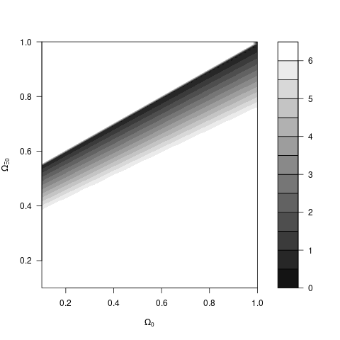
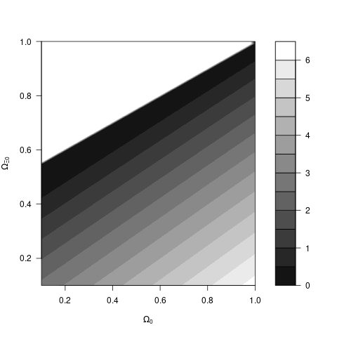
Figure 1: Function $\Delta(\Omega_{0},\Omega_{\Xi 0})=\chi^{2}_{\nu}-\chi^{2}_{\nu\mathrm{min}}$, the difference between $\chi^{2}_{\nu}$ (Eq. 150) and its minimum value, for the CRG+ (left panel) and the CRG– (right panel) solutions. Under the assumption of Gaussian random errors, the 68%, 90%, 95%, and 99% confidence regions of the two parameters are the area where $\Delta(\Omega_{0},\Omega_{\Xi 0})<2.3$, $4.6$, $6.2$, and $9.2$, respectively. The 90% confidence regions are thus $0.43+0.44\Omega_{0}\lesssim\Omega_{\Xi 0}\leq 0.5(1+\Omega_{0})$ for the CRG+ solution and $\max\{0,(-0.26+0.63\Omega_{0})\}\lesssim\Omega_{\Xi 0}\leq 0.5(1+\Omega_{0})$ for the CRG– solution. In the two panels, there are no solutions in the white top left area. For the CRG+ solution shown in the left panel, for an easier comparison with the CRG– solution shown in the right panel, $\Delta(\Omega_{0},\Omega_{\Xi 0})$ is not reported in the white bottom right area where $\Delta>7$.

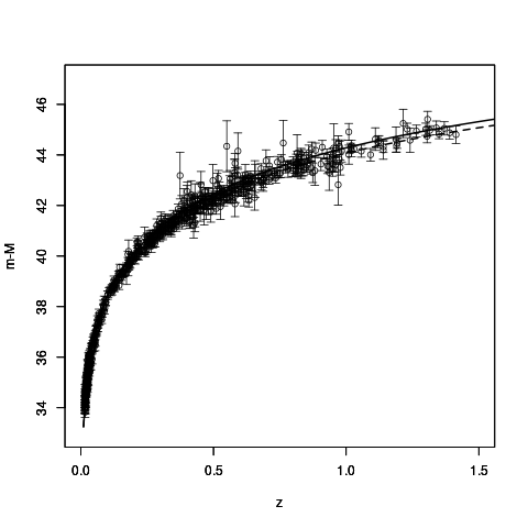
Figure 2: Hubble diagram of the SNIa data (open circles with error bars) and the CRG+ (solid line) and CRG– (dashed line) solutions. For the two curves, we adopt $H_{0}=67.7$ km s^-1 Mpc^-1, $\Omega_{0}=0.31$, and $\Omega_{\Xi 0}=0.65$.

Appendix F The equation of state of the effective dark energy

The equation of state of the effective dark energy can be calculated by inserting Eqs. (65)-(66) into Eqs. (71)-(72). For a dust-dominated universe, we can use Eqs. (52) and (54) to calculate $\varphi$, $\dot{H}$, and the following quantities

$$\dot{\varphi} =-\frac{H_{0}\varphi_{0}}{a^{3}}\left(\frac{\dot{H}}{H^{2}}+3\right)\,,$$ (151)

$$\ddot{\varphi} =\frac{H_{0}\varphi_{0}}{a^{3}}\left(-\frac{\ddot{H}}{H^{2}}+2\frac{\dot{H}^{2}}{H^{3}}+3\frac{\dot{H}}{H}+9H\right)\,,$$ (152)

$$\ddot{H} =\frac{3}{2}\left(4H^{3}+3\Omega_{0}H_{0}H^{2}-4\Omega_{\Xi 0}H_{0}^{2}H\right)\,.$$ (153)

The combination of these results, together with the two definitions of the cosmological parameters Eqs. (40)-(41), yields

$$w_{\mathrm{DE}}=\frac{3H^{2}\pm 2\sqrt{3}\left(H^{4}+\Omega_{0}H_{0}H^{3}-2\Omega_{\Xi 0}H_{0}^{2}H^{2}\right)^{1/2}}{-3H^{2}+3\Omega_{0}H_{0}H/2-\left[(Ha^{3}/H_{0})-1\right](3H_{0}^{2}/2a^{3})\Omega_{0}}\,.$$ (154)

The upper and lower signs refer to the CRG+ and the CRG– solutions, respectively. We use this equation in Sect. 4.3.