Simultaneous ALMA−Hinode−IRIS observations on footpoint signatures of a soft X-ray loop-like microflare

Abstract

Microflares have been considered to be among the major energy input sources to form active solar corona. To investigate the response of the low atmosphere to events, we conducted an ALMA observation at 3 mm coordinated with IRIS and Hinode observations, on March 19, 2017. During the observations, a soft X-ray loop-type microflare (active-region transient brightening) was captured using Hinode X-ray telescope in high temporal cadence. A brightening loop footpoint is located within narrow field of views ALMA, IRIS slit-jaw imager, and Hinode spectro-polarimeter. Counterparts of the microflare at the footpoint were detected in Si IV and ALMA images, while the counterparts were less apparent in C II and Mg II k images. Their impulsive time profiles exhibit the Neupert effect pertaining to soft X-ray intensity evolution. The magnitude of thermal energy measured using ALMA was approximately 100 times smaller than that measured in the corona. These results suggest that impulsive counterparts can be detected in the transition region and upper chromosphere where the plasma is thermally heated via impinging non-thermal particles. Our energy evaluation indicates a deficit of accelerated particles that impinge the footpoints for a small class of soft X-ray microflares. The footpoint counterparts consist of several brightening kernels, all of which are located in weak (void) magnetic areas formed in patchy distribution of strong magnetic flux at the photospheric level. The kernels provide a conceptual image in which the transient energy release occurs at multiple locations on the sheaths of magnetic flux bundles in the corona.

1 Introduction

The solar corona is formed at more than $10^{6}$ K above the surface (photosphere) with a temperature of 6,000 K. The corona is highly structured and has active regions with high energy input that are observed to be bright and active in soft X-rays and high-temperature extreme ultraviolet (EUV) lines. Small-class transient reconnection events, that is, microflares (in the order of $10^{27}$ erg) and nanoflares (in the order of $10^{24}$ erg), have been considered to be among the major energy input sources to form the active corona. This is because extremely high temperature plasma ($>8$ MK) is observed in active regions (Yoshida and Tsuneta, 1996; Teriaca et al., 2012). Microflares have been predominantly observed as transient brightenings in active regions (Shimizu et al., 1992) that morphologically show various brightening coronal structures in soft X-rays (Shimizu et al., 1994). Simultaneous multiple loop brightenings are more often seen than single loop brightenings and the loops tend to brighten either from their footpoints and/or from the the apparent contact point , followed by the brightening of the entire loops. In such cases, the energy release site is located in the corona. Certain portion of the energy released in the corona is transported via accelerated particles and thermal conduction along the magnetic field to the footpoints, where the chromospheric and transition region cool plasma is transiently heated. We are yet to understand the partition of the energy; the amount of energy transferred to the footpoints and significant heating of the chromosphere. Studies have been conducted on the energy partition in flares (references in Section 4.3). Observational understanding of the energy partition in microflares and nanoflares can significantly expand the range of energy to disucss the energy partition. This helps to understand the energy partition changes as a function of event energy size.

The energy released by small-scale transient events has been evaluated as thermal energy via temperature and density diagnostics using soft X-ray or EUV intensities. This provides frequency distribution in microflare and nanoflare energy range (Shimizu, 1995; Aschwanden et al., 2000, and references herein). Hard X-ray observations are also used to evaluate non-thermal energy; however, they are solely conducted for flares above $5\times 10^{28}$ erg (Crosby, Aschwanden and Dennis, 1993). The hard X-ray emission originated predominantly in the accelerated particles that impinge the lower atmosphere at the footpoints of the magnetic structure of coronal flaring. The Interface Region Imaging Spectrograph (IRIS)(De Pontieu et al., 2014), launched in 2013, has a high-resolution used to observe the movement of heat and energy in the chromosphere and lower portion of the coronal transition region. IRIS has a spectrograph and slit-jaw imagers to monitor the intensity of some wavelength bands that contain spectral lines originating from the chromosphere and lower portion of transition region. Later in the decade following 2010, a new diagnostic capability for the chromosphere was incorporated when the Atacama Large millimeter and sub-millimeter Array (ALMA) (ALMA Partnership, 2016) began solar observations. ALMA can perform interferometric observations of the Sun at millimeter (mm) wavelengths. Most of the mm emission comes from the chromosphere (Vernazza et al., 1981). The mm-wavelength emission is a free-free emission (thermal bremsstrahlung) produced by free electrons scattering off ions without being captured. The free electrons can be assumed to be in local thermodynamic equilibrium: thus, the source function is equivalent to the Plank function. In the mm wavelengths, the Rayleigh–Jeans law is an approximation to the Plank function that demonstrates a linear relationship between the emission intensity and the brightness temperature (Kraus, 1986). This indicates that the radiation at mm wavelengths can be used as a thermometer to probe the chromospheric temperature. The thermometer provides acts as a useful tool to detect changes in the chromospheric temperature to estimate the amount of energy transferred to the chromosphere.

In this study, we present the first example of small-scale transient brightenings produced in the solar corona (hereafter, referred to as soft X-ray microflare) and their responses in the chromosphere and lower portion of coronal transition region. The soft X-ray microflare was captured in high temporal cadence using Hinode X-ray telescope to observe the evolution of brightening loop structure in the corona and locations of the brightening loop footpoints on the solar surface. One footpoint was within the narrow fields of view of the ALMA, IRIS, and Hinode spectro-polarimeter. The spectro-polarimeter provides high precision and high spatial resolution maps of magnetic flux distributed on the photosphere, which are helpful to understand the magnetic field configurations of the soft X-ray microflare.

This article is organized as follows. Section 2 describes the observations and data analysis. Section 3 presents the results of the data analysis. Section 4 and Section 5 present the discussion of the results and summary, respectively.

2 Observations and Data analysis

2.1 Observations

A coordinated observation was conducted among the ALMA, IRIS, and Hinode on March 19, 2017. The ALMA project, with project code 2016.1.00030.S (PI: Shimizu), was executed. The Hinode and IRIS operation plan was numbered as IHOP 327. We selected a tiny active region located in the eastern hemisphere on the solar disk as the observing region for the coordinated observations. The region is seen as a compact bright region in the soft X-rays; it exhibits a magnetic bipolar distribution on photospheric SDO/HMI magnetograms.

The ALMA observation was conducted at 100 GHz (Band 3) from 15:33 to 19:10 UT. The observation consists of three runs (15:33–16:26 UT, 16:53–17:46 UT, and 18:16–19:10 UT); a soft X-ray microflare occurred during the first run. This tiny active region is located at ($-495$″, $-40$″) on the heliocentric coordinate at the beginning of the first run. The antenna layout is the C40-1 configuration, which is the most compact layout in the solar observing mode with sets of 39 and 7 antennas with diameters 12 m and 7 m, respectively. The longest baseline is 249 m with a spatial resolution of $5.0\times 3.9\arcsec$. The common astronomy software applications (CASA Ver 5.4; McMullin et al., 2007) was used to calibrate and image the data. The CLEAN procedure ’tclean’ was used to synthesize each image (Shimojo et al., 2017). The synthesis was conducted excluding the visibilities between the two antenna sets (39 and 7 antennas) because appropriate synthesis was not obtained when all the visibilities among the antennas were used. When the $7-12$ m baselines were involved in the synthesis, artificial stripes appeared in the synthesized images. The stripes disappeared when the baselines were removed. We do not appropriately understand the origins of the stripes; however, the visibility data of $7-12$ m baselines degraded the image quality. Careful calibration might solve this issue; however, we removed the baselines in the image synthesis presented in this study because we do not know the calibration process for the $7-12$ m baselines. The data were self-calibrated in phase. The self-calibration process has five steps with different accumulating periods to obtain the solution from 10 min for the first step to 2 s for the last step such that the temporal cadence is 2 s in this study. No single dish (total power) data were acquired to calibrate the absolute brightness temperature in this observation. Thus, the temporal profiles presented in this article show the deviation from the averaged brightness temperature in the observation field-of-view. The increase in temperature brightness for the event considered can be derived even without absolute temperature information.

The IRIS satellite performed the spectroscopic and slit-jaw imaging observations during the period. This article presents the results obtained from the slit-jaw images because the slit positions were not present around the footpoint of the soft X-ray microflare. The slit-jaw images were acquired at three channels 1400, 1330, and 2796, each of which covers Si IV 1394/1402 Å lines ($10^{4.8}$ K), C II 1335 Å lines ($10^{4.2}$ K), and Mg II k line ($10^{4.0}$ K), respectively, at a cadence of 22 s. The pixel size is $0.34\arcsec$. Each image has a field of view of $60\times 65\arcsec$, but it moves in the EW direction at each exposure because of the scanning for spectroscopic measurements. This provides the maximum coverage in the field of view, at $120\times 65\arcsec$. The level 2 data from the IRIS were used in this analysis, which were obtained following instrumental calibration including dark current, flat field, and geometric corrections.

The X-Ray Telescope (XRT) (Golub et al., 2007; Kano et al., 2008) on the Hinode satellite (Kosugi et al., 2007) repeatedly and continuously acquired Al-poly filter images every 4 s with occasional exposures of G-band images (XOB #1B76). The image size is $128\times 128$ pixels with a pixel scale of $1.031\arcsec$(Shimizu et al., 2007). The standard calibration routine on Solar SoftWare was used to calibrate the time series of the XRT images.

The Hinode’s Solar Optical Telescope (SOT) (Tsuneta et al., 2008; Suematsu et al., 2008; Shimizu et al., 2008; Ichimoto et al., 2008) repeatedly and continuously recorded the full-polarization states of line profiles of two magnetically sensitive Fe I lines at 630.15 and 630.25 nm using the spectro-polarimeter (SP, Lites et al., 2013). The fast-mapping mode was used, which covers a $77\times 80\arcsec$ field of view with an effective pixel size $0.32\arcsec$. The spectral sampling is 21.549 mÅ pixel^-1. The map cadence was approximately 30 min. We used the SOT/SP level 2 databasefromthe Community Spectro-polarimetric Analysis Center (CSAC) at HAO/NCAR, which are results ofMilne–Eddington inversions by the MERLIN code with the calibration described in Lites & Ichimoto (2013).

2.2 Image Co-alignment and Spatial Distribution Correspondence

The data from the different instruments were carefully investigated to identify a better method for the co-alignment; we finally achieved better than $2\arcsec$ in the uncertainty of the co-alignment. IRIS and Hinode data were mapped on the full Sun images from the Solar Dynamic Observatory (SDO, Pesnell et al., 2012) by obtaining the maximum correlation between the corresponding data; A Hinode SP map was mapped on the HMI magnetogram (Scherrer et al., 2012; Schou et al., 2012) by obtaining the best matching in the spatial distribution of the magnetic flux. The time series of the Hinode XRT images were mapped on an AIA 94 Å coronal image to determine the co-alignment accuracy. The IRIS slit-jaw images were mapped on the AIA 1600 Å chromospheric image using an image of 2794 Å. For the ALMA data, the coordinates available for each map were used to co-align to the SDO full-sun images because the pointing accuracy of the ALMA antennas has been established as more than $2\arcsec$ (ALMA Partnership, 2016). Nevertheless, the coordinates of the image provided by the ALMA observatory exhibit a problem when the coordinates are not appropriately revised using the reference time. Generally, the coordinates are not revised when there is no pointing data that are derived from the encoders of the antennas. To avoid this problem, we revised the coordinate using the reference time, which differs from that mentioned in the readme file of the data package in the ALMA Archive.

Figure 1 shows the spatial distribution of features in the co-aligned images. The SP line-of-sight magnetic flux density map (Figure 1(a)) demonstrates a bipolar flux distribution in the field of view. The areas where the magnetic flux is concentrated are brighter than their surroundings in the three IRIS slit-jaw images (Figure 1(c)–(e)). Brighter features in the IRIS images correspond to small flux concentrations. Diffuse features can be recognized around the bright features, which may be caused owing to the expansion of magnetic flux at the chromospheric height. Bright features at flux concentrations mean that high heating rate is sustained from the middle chromosphere to a lower portion of the transition region at the magnetic flux concentrations; the temperature responses of the Mg II, C II, and Si IV filters are at peak values in the middle chromosphere ($10^{4.0}$ K), upper chromosphere ($10^{4.2}$ K) and a lower portion of the transition region ($10^{4.8}$ K), respectively. Figure 1(b) shows the corresponding ALMA brightness temperature map, which is time-averaged over the first run. The brightness temperature here is the deviation from the temperature averaged over the field of view. The overall spatial distribution in the ALMA temperature map corresponds well with those observed in the IRIS chromospheric maps. However, the ALMA map shows a more diffuse distribution, which may be because of the lower spatial resolution of the ALMA in this observation. Figure 1(f) is a co-aligned X-ray image. The bright corona is not observed as a bipolar structure connecting the flux concentrations to each other, which is completely different from what is observed in the chromosphere and lower transition region.

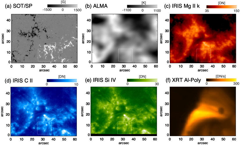
Figure 1: Spatial distribution of time-averaged features visible in (a) SP line-of-sight magnetic flux density, (b) ALMA brightness temperature, (c) IRIS slit-jaw Mg II filter, (d) IRIS slit-jaw C II filter, (e) IRIS slit-jaw Si IV filter, and (f) Hinode XRT Al-poly filter. They are co-aligned to each other according to the method described in section 2. In (a), the white and black are positive and negative polarities, respectively. Solar north is upwards and west is to the right direction. DN is data number units.The boxes show the field of view of Figures 4 and 5.

3 Results

3.1 Loop-like Microflare in Soft X-rays

Figure 2 shows the time series of soft X-ray images (with Al-poly filter) obtained from the Hinode XRT. Six frames were selected from the cadence series of images at 4 s to show the occurrence of a loop-like microflare, which is located almost at the center of the images. A single coronal loop became apparent up to the 4th frame (15:54:41 UT), which was the time when the intensity was at peak. This loop brightening started from 15:51 UT immediately after the 1st frame, in which a couple of loop structures had been faintly visible previously. Another loop structure existed at the right side parallel to the brightening loop considered; it may have been extended towards the west direction. This structure showed a temporal evolution similar to that of the brightening loop. Figure 3 (a) shows the time profile of the soft X-ray intensity for the area identified with light blue lines in Figure 2. The vertical dashed lines represent the time at which each frame in Figure 2 was acquired. The intensity stayed at a constant level until 15:51 UT (1st frame in Figure 2), followed by a transient increase in the intensity. The intensity required approximately 3 min to attain its peak at 15:54:30 UT (4th frame in Figure 2). The increased total intensity of the brightening loop is $5.8\times 10^{3}$ DN s^-1, where DN is data number.Itwas derived by integrating the pixels surrounded by the light blue lines in Figure 2(c). Then, the intensity gradually decreased and required approximately 10 min to attain the minimum. This temporal evolution is conventional for the soft X-ray behaviors observed well in the solar flares and microflares.

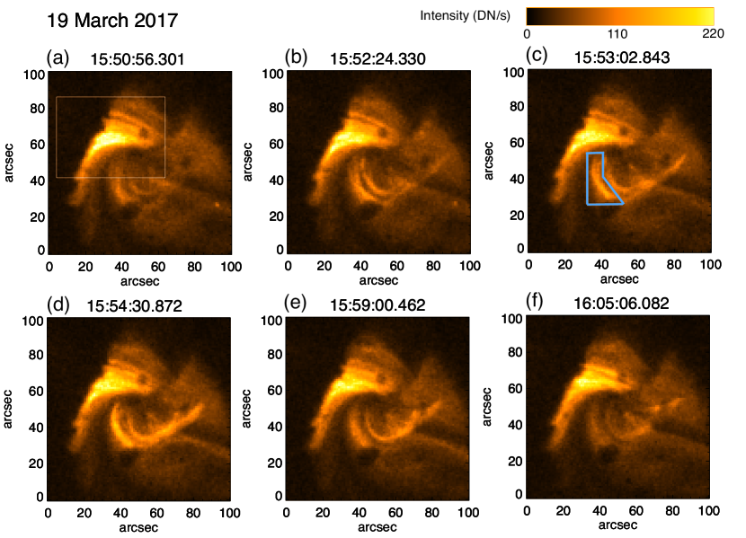
Figure 2: Time series of soft X-ray images (Al-poly filter) acquired by Hinode X-Ray Telescope. The time sequence is from (a) to (c) and then from (d) to (f). The field of view is wider than that in Figure 1. Solar north is upwards and west is to the right direction. The rectangle in (a) shows the field of view used in Figure 1. The area surrounded by light blue lines in (c) indicates the pixels where the intensity was integrated for Figure 3(a).

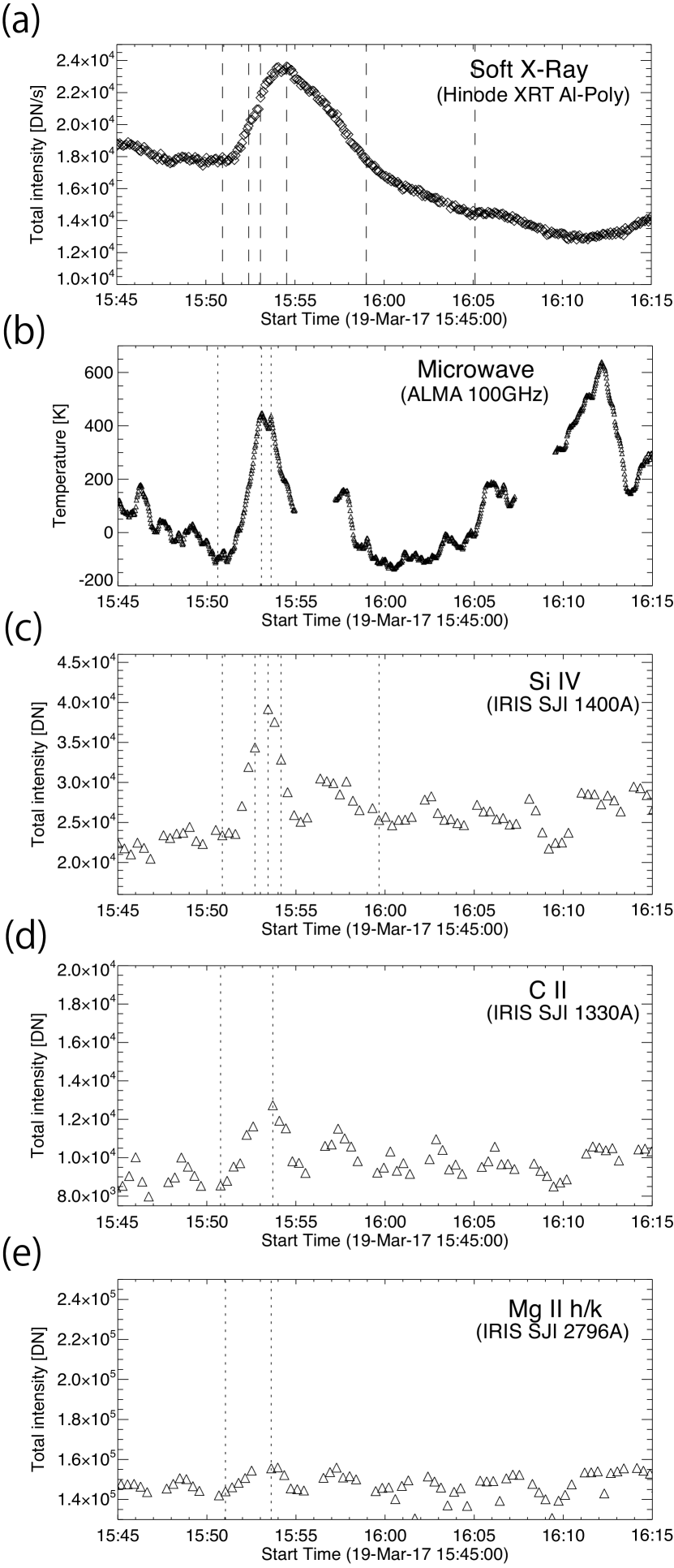
Figure 3: Intensity profiles of (a) the soft X-ray microflare and its counterparts measured in (b) 100 GHz, (c) Si IV, (d) C II, and (e) Mg II k. The counterparts were measured at one of the footpoints of the soft X-ray brightening loop, while the soft X-ray profile is for the entire area of the brightening loop, as specified in Figure 2. The vertical dash lines determine the time of the images shown in Figures 2, 4 and 5.

One of the brightening loops, that is, the upper (north) end of the loop, is located within the observing fields of view of IRIS, ALMA, and Hinode/SP such that we can investigate the behaviors of the footpoint at different wavelengths. Figure 3(c) shows the area intensity profile in the Si IV slit-jaw channel of the IRIS. The Si IV intensity began to increase at 15:52 UT and peaked at 15:53:25 UT, followed by an immediate decrease of the intensity to the initial level by 15:55 UT. This transient intensity increase is faster than the ascending slope in the soft X-ray profile (Figure 3(a)); the increased Si IV intensity quickly reduced before reaching the peak in soft X-ray.

Some Si IV images are shown in Figure 4, whose acquired times are identified by the vertical dash lines in Figure 3(c). The field of view is $13.3\times 11.6\arcsec$, where the loop footpoint is located around the center. As described in Section 2, a $60\times 65\arcsec$ field was repeatedly moved in the EW direction at each exposure to sample spectral lines at several positions in the $120\times 65\arcsec$ field of view. Because of this operation, observing field of view changed with time, which can be partly recognized in the 2nd and 3rd frames as the dark area. Four or five bright kernels, each of which has a size of less than $1\arcsec$, appeared in the 2nd frame (15:52:41 UT). In the 3rd frame (15:53:25 UT), that is, at the peak time, the bright kernels showed a slight increase in intensity, location, and shape. However, we recognized two bright kernels at similar locations. The frame at the lower right shows the intensity difference in the 3rd frame when compared with the 1st frame (15:50:51 UT). This clearly provides the location of brightening features at the footpoint of the soft X-ray microflare. The bright features may be grouped into two areas centered at (X, Y) = (5.5, 4) and (8, 6) in arcsec.

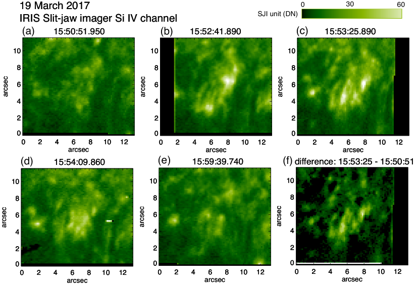
Figure 4: Si IV channel images from the IRIS slit-jaw imager for the five times specified in Figure 3. The 1st frame (a) is before the intensity began increasing, and the 3rd frame (c) is at the intensity peak. The frame (f) is obtained from the difference between (a) and (c). The field of view is $13.3\times 11.6\arcsec$ and its location is shown in Figure 1.

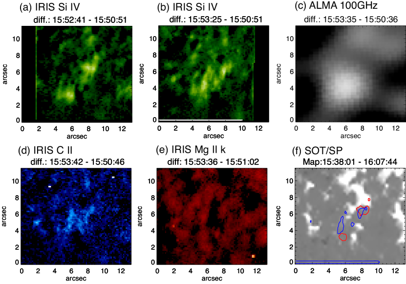
Figure 5: Difference frames for (a), (b) Si IV, (c) 100 GHz, (e) C II, and (f) Mg II k, which were obtained by subtracting the background image (identified by the 1st vertical dash line for each time plot shown in Figure 3). The frames in (b), (c), (d), and (e) are for the images recorded at peak time. (f) Spatial distribution of the magnetic flux density derived from the Hinode SP scan in 15:38:01–16:07:44 UT. The red and blue contours indicate the position of Si IV bright kernels observed in (a) and (b), respectively. The field of view is same as that of Figure 4.

Figure 3(b) is the temporal evolution of the brightness temperature at 100 GHz for the region considered, which shows that the counterpart signals are detected by ALMA at 100 GHz. The ALMA temporal profile of the brightness temperature is almost same as that in the Si IV channel. The intensity increase is also visible in the C II channel, as shown in Figure 3(d), but not in the Mg II k channel (Figure 3(e)). Figures 5 (b), (c), (d), and (e) show the Si IV, 100 GHz, C II, and Mg II k images, respectively, at the intensity peak time with the background removed. The background is the frame specified by the 1st vertical dash line in each time plot in Figure 3. The counterparts are clearly detected in Si IV and 100 GHz at 15:52–15:53 UT. The spatial resolution of the ALMA data is at least 10 times lesser than that of the IRIS. Although the intensity is weak, the counterparts can be observed in the C II frame. No apparent counterpart is observed in the Mg II k frame.

Figure 5(f) is the spatial distribution of magnetic flux at the photosphere. Almost all the bright kernels observed in Si IV and C II are located in weak, void areas surrounded by strong magnetic flux concentrations, as shown by the contours.

3.2 Thermal energy of the soft X-ray microflare

Using the total soft X-ray intensity at the time of its peak intensity, we estimated the thermal energy content for the soft X-ray microflare. The thermal energy content $E_{th}$ is

$$E_{th}=3n_{e}k_{B}TV,$$ (1)

where $n_{e}$ is the electron density, $k_{B}$ is the Boltzmann constant, $T$ is the electron temperature, and $V$ is the volume. In the Yohkoh era, many studies used a filter ratio method for the temperature and density by assuming isothermal plasma (e.g. Shimizu, 1995; Shimojo and Shibata, 2000), followed by more advanced techniques, such as differential emission measure. In this observation, only Al-Poly filter images were acquired to obtain dynamical behaviors with high temporal cadence. Thus, we used the method proposed by Sako (2014) to estimate the order of energy. This method states that the thermal energy is not sensitive to the temperature of the XRT filter intensities. The filter response curve $R(T)$ is simplified to be

$$R(T)=\frac{I}{\int n_{e}^{2}dV}\approx\frac{I}{n_{e}^{2}V},$$ (2)

where $I$ is the measured total soft X-ray intensity. Thus, the thermal energy content can be described as

$$E_{th}=3\sqrt{\frac{I}{R(T)V}}k_{B}TV=3k_{B}\sqrt{\frac{T^{2}}{R(T)}}\sqrt{IV}.$$ (3)

The response curve of the Al-poly filter is approximately a power-law distribution as a function of temperature in $10^{6}-10^{7}$ K (Golub et al., 2007). If the power-law index is 2, $R(T)$ is proportional to $T^{2}$. Thus, $E_{th}$ is insensitive to the temperature. The Al-poly filter exhibits a power-law index approximately equal to 2, that is, it exhibits a very weak dependence on the temperature, as shown in Figure 6. In our estimation, we used $1.1\times 10^{38}$ K² s pixel DN^-1 cm^-5 for $T^{2}/R(T)$, which is the average of $4-8$ MK. Transient brightenings in active regions have conventionally exhibit a temperature of $4-8$ MK (Shimizu, 1995). The $T^{2}/R(T)$ has an error range of $1.0\times 10^{38}-1.2\times 10^{38}$ in the energy estimation. The volume of the brightening loop was determined by measuring the length ($l$ = 27”) and width ($w$=3.7”) of the loop. Assuming that the depth (the length of line-of-sight) of the loop is equal to the width, we simplified the volume $V$ as $l\times w^{2}$. The XRT pixel size (1”) was used for error estimation. This calculation obtained a volume of $1.4\times 10^{26}$ cm³ with an uncertainty range between $0.75\times 10^{26}$ cm³ and $2.4\times 10^{26}$ cm³. Therefore, the thermal energy content was estimated to be $2.9\times 10^{26}$ erg with an uncertainty range between $2.0\times 10^{26}$ erg and $4.0\times 10^{26}$ erg. The thermal energy produced by the microflare in the corona is larger than the thermal energy content because the thermal energy content is the amount of the thermal energy at a single time (peak time) without considering energy losses from the radiation and thermal conduction during the ascending phase (Shimizu, 1995).

Figure 6: $T^{2}/R(T)$ as a function of temperature ($T$) for the XRT Al-Poly filter, where $R(T)$ is the filter response curve.

3.3 Thermal energy measured at the chromosphere

The ALMA data can provide an order estimate of the thermal energy supplied to the chromosphere to which the 100 GHz microwave is sensitive. Here, we assumed that the ALMA signal is the thermal free-free radiation. As observed from Figure 3, the ALMA signal was peaked during the ascending phase of the soft X-ray emission. No polarization was measured using ALMA in this observation; thus, we cannot ignore gyro-cynchrotron radiation for the transient enhanced signal at the footpoint in the ALMA data. Nevertheless, we interpreted it as the signal caused by the thermal plasma heated in the chromosphere by the electrons that are predominantly impinging the chromosphere.

The thermal energy supplied to the chromosphere is evaluated as the thermal energy content $E_{ch}$, which is

$$E_{ch}=3n_{e}k_{B}\Delta TV,$$ (4)

where $\Delta T$ is the excess in electron temperature. (Nindos et al., 2020). Because the brightness temperature is a reasonable measure of the gas temperature at an effective formation height in the chromosphere (Loukitcheva et al., 2015), for the increase in electron temperature, we obtained the increase in brightness temperature above the background level at the time when the ALMA time profile was at its peak. The ALMA application (CASA) derived the flux density defined as the integration of brightness over the antenna beam angle in the units of Jansky per beam size. Assuming that the beam is Gaussian, the flux density was converted to brightness temperature, according to the formula presented in ALMA Cycle 4 Technical Handbook. The background level is the brightness temperature just before the event, whose time is identified by the left most dashed line in Figure 3(b). The increased brightness temperature derived was 545 K.

The electron density was assumed to be in the order of $10^{11}$ cm^-3 according to certain numerical modeling efforts. Loukitcheva et al. (2015) derived that the range of brightness temperature for an active-region magnetic structure is from 2,945 K to 13,104 K with an average of 6,090 K and root mean square variation of 1,333 K for the 100 GHz radiation. The 100 GHz (3 mm) radiation has effective formation height of approximately 1,500 km with a contributing range of $1,200-2,000$ km depending on the magnetic structures, where the electron density is approximately $10^{11}$ cm^-3.

The volume used in the evaluation was determined by assuming that the area where the 100 GHz radio emission is in excess during the event was almost same as the footpoint area of brightenings clearly detected in the Si IV (Figure 4). The upper left frames in Figure 5 indicate that the footpoint area changed from image to image. For simplicity, we selected $8\arcsec$ for the N-S direction and $5\arcsec$ for the E-W direction to cover the entire area of various footpoints $A$ with $\pm 1\arcsec$ for uncertainty evaluation. Assuming that the extent in the height is comparable to the horizontal size, the volume $V$ was estimated to be $A^{3/2}$. This might be an overestimation because the effective height of the 100 GHz radio is 800 km (approximately $1\arcsec$). However, the transient heating by impinging electrons at the chromosphere may expand the heated plasma towards the upper layers. With these parameters, we obtained $(2.2\pm 1.2)\times 10^{24}$ erg as the thermal energy supplied to the chromosphere.

4 Discussions

In this article, we investigated the heating of the footpoints using IRIS and ALMA when an energy of $2.9(\pm 1.0)\times 10^{26}$ erg was transiently released in coronal structure that is observed as a single brightening loop using the Hinode XRT. Counterparts were clearly detected in the Si IV and ALMA at 100 GHz. They are visible but less apparent in the C II, and it is difficult to distinguish them in the Mg II k. Their time profiles were impulsive; the intensities attained their peaks at approximately 1.5 min before the peak of the soft X-ray intensity was attained. This was followed by a prompt decrease in intensity in a few minutes. This temporal behavior is similar to the Neupert effect (Neupert, 1968), which has been observed in (non-thermal) hard X-rays pertaining to the soft X-ray (thermal) temporal behavior. Moreover, the exact position of the footpoints was identified with high spatial resolution maps of the magnetic flux density at the photosphere from the Hinode SOT/SP with a spatial relation to bright kernels in Si IV. Almost all the bright kernels are located in weak, void areas surrounded by strong magnetic flux concentrations.

4.1 Height dependence

The Si IV (1400 Å ) filter is dominated by the Si IV 1394/1402 Å lines with the continuum. The continuum is sensitive to the upper photosphere and low chromosphere, but the Si IV lines are formed at an equilibrium temperature of approximately 80,000 K, which corresponds to the temperature in the transition region (Peter et al., 2014). The C II (1330 Å ) filter is dominated by C II lines at 133.5 nm (upper chromosphere) with the continuum while the Mg II k (2796 Å ) filter dominates the Mg II k (chromosphere) and inner wings (photosphere). The C II and Mg II k lines are formed at similar heights below the transition region, but the C II lines can be formed at a height higher and lower than the core of the Mg II k line depending on the quantitative measure of the materials in the temperature range of 14,000 – 50,000 K. Significant amounts of materials in this temperature range form the C II lines at a height higher than that of the Mag II k line core (Rathore and Carlsson, 2015; Rathore et al., 2015).

Certain studies derived the mean brightness temperatures (with standard deviation) of the 3 mm ALMA band 7,300 ($\pm 100$) K (White et al., 2017), 7,250 ($\pm 170$) K (Alissandrakis et al., 2017) for the disk center, and 7,250 ($\pm 1,140$) K (da Silva Santos et al., 2018) for radiative magnetohydrodynamics (MHD) simulation of an enhanced network region. da Silva Santos et al. (2018) studied the diagnostic potential of combined optical, ultraviolet, and ALMA observations and showed that the response function to temperature is at maximum at log $\tau=-5.6$, distributed between log $\tau=[-6.0,-5.1]$, which is slightly higher or almost same as that of the Mg II k line core, that is, the maximum at log $\tau=-5.5$, distributed between log $\tau=[-6.4,-5.1]$, where $\tau$ is optical depthat 500 nm.

From these studies, we can interpret that the order of the mean temperature is Si IV, C II, 100 GHz, and Mg II k from higher to lower temperatures. Furthermore, C II, 100 GHz, and Mg II k are distributed in a small temperature range at the upper chromosphere but below the transition region. Considering the temperature distribution models of the solar atmosphere as a function of height, the Mg II k image is located at the lowest height, followed by 100 GHz, C II, and Si IV toward the upper heights. This order of heights, with particles impinging from the corona to the chromosphere, can explain the observation at one of the footpoints for the soft X-ray microflare, that is, more apparent signals were observed at Si IV, 100 GHz, C II, and Mg II k, respectively.

4.2 Thermal energy supplied to the chromosphere

In Section 3.3, the thermal energy supplied to the chromosphere was estimated on the assumption of thermal free-free radiation. The increased brightness temperature from the ALMA signal was used for the excess in electron temperature. This is valid when the optical thickness is unity or larger, i.e., optically thick, at 100 GHz. The relationship between brightness temperature and electron temperature can be written as

$$T_{b}=T_{e}(1-e^{-\tau_{100}}),$$ (5)

where $\tau_{100}$ is the optical thickness at 100 GHz (Kraus, 1986). As the optical thickness decreases, the brightness temperature becomes smaller than the electron temperature. For the optical thickness much smaller than the unity, the brightness temperature can be approxiated by $\tau_{100}T_{e}$.

Alissandrakis et al. (2020) measured the brightness temperature from ALMA center-to-limb observations at 100 GHz for magnetic bright networks. From the inversion of this measurement, the electron temperature was derived as a function of the optical thickness at 100 GHz for magnetic bright networks, giving $7,383-7,916$ K where the optical thickness is unity at 100 GHz. They also computed the electron temperature as a function of the optical thickness using opacity from the model parameters of Model F, characterized as very bright network element, of the FAL93 (Fontenla et al., 1993) model. The Model F gives the electron temperature of 9,200 K for the optical thickness of unity at 100 GHz. These values are only $0-25$ % increase from the mean brightness temperatures at 100 GHz (Section 4.1) and thus equation (5) provides that the optical thickness is about unity or higher. With this assessment, we conclude no big difference for the order estimation of thermal energy supplied to the chromosphere event if the brightness temperature is used as the electron temperature. Similar treatment is applied by Nindos et al. (2020, 2021), which derived the energy of transient brightenings observed in the quiet Sun with ALMA.

We assumed thermal free-free radiation for the signals detected with ALMA. Kontar et al. (2018) examined mm and UV radiations from bright flare ribbons observed at various M- and X-class flares and showed that mm radiation (including 100 GHz) is consistent with free-free radiation from the plasma of flare ribbons at temperatures $10^{4}-10^{6}$ K, providing the assumption is reasonable for the order estimation of a much smaller energy releasing event examined in this study. However, the plasma may be in a dynamic state due to the transient response of the flux of impinging particles, which can deviate largely the mm radiation from what is expected by thermal free-free radiation. As Morgachev et al. (2020) points out, it is important to consider not only thermal flare plasma emission but also dynamics of accelerated electrons and nonequillibrium effects on radiation transfer. Better understanding of these effects would predict the intensity of the radiation at 100 GHz more accurately and improve the accuracy of the energy estimation. Such efforts will enhance the validity of the energy obtained in this study.

4.3 Energy partition

The thermal energy supplied to the chromosphere was estimated at $(2.2\pm 1.2)\times 10^{24}$ erg with the 100 GHz measurement. This is only 1% of the thermal energy observed at the peak time of the soft X-ray brightening loop in the corona, $(2.9\pm 1.0)\times 10^{26}$ erg. It is only 2% even when the same amount of energy was transported to the two footpoints of the coronal loop. Considering the temporal evolution of 100 GHz signals with respect to the soft X-ray thermal evolution, the thermal energy from the 100 GHz measurement is created by the particles impinging the dense layers. Thus, this estimated energy can be regarded as the energy exhibited by non-thermal accelerated particles required for the order estimation. The energy partition between the thermal and non-thermal plasmas in solar flares has been an important issue in the physics of magnetic reconnection and particle acceleration. For example, Emslie et al. (2004) evaluated the energy budget for two X-class flares/CME events and showed that the peak energy in the thermal soft X-ray plasma (in the order of $10^{31}$ erg) is approximately one order of magnitude less than the energy in the accelerated particles. Saint-Hilaire and Benz (2002) also evaluated that the thermal energy of the flare kernel (approximately $10^{29}$ erg) was more than an order of magnitude smaller than the electron beam energy for a smaller (C9.7 class) compact flare. More recent studies reported the energy partition for more numbers of flares (Stoiser et al., 2007; Emslie et al., 2012; Inglis and Christe, 2014; Warmuth and Mann, 2016a, b; Aschwanden et al., 2017). However, they provided contradicting results on energy partition, particularly for weak flares. For A- and B-class flares, Inglis and Christe (2014) derived the ratio of nonthermal energy and peak thermal energy at a few times of $10^{-1}$ for 10 events, whereas Stoiser et al. (2007) obtained $10^{1}-10^{2}$ from 18 events. Warmuth and Mann (2020) reviewed these studies and identified uncertainties in deriving the energy partition. Considering these studies together with the identified uncertainties, they suggested that the thermal–nonthermal energy partition changes with the flare importance; a deficit of energetic electrons is observed in weak flares,while the nonthermal energy is sufficient to account for the thermal component in strong flares. However, we did not evaluate the energy partition for much smaller events.

Our observation detected one microflare with various instruments to discuss the energy partition. However, it is only one event. Our result may suggest that energetic electrons are much less generated when the magnitude of energy release events decreases to the small energy group of microflares, that is, $10^{26}$ erg. It is in the order of $10^{-2}$ in the case of the event examined. Less number of energetic electrons may also mean that the heights that the energetic electrons can impinge to are not low. Battaglia and Kontar (2011) showed that the hard X-ray emission at 30 keV is approximately 1,000 km above the photosphere. Moreover, the energy deposition rate as a function of height for two different cases of electron cutoff energy shows that the electrons of $12-20$ keV predominantly release the energy at $2,000-3,000$ km. These heights correspond to the upper chromosphere or lower transition region with a density of between $10^{11}$ cm^-3 and $10^{12}$ cm^-3, where the Si IV line can be formed when compared to radio at 100 GHz, C II and Mg II k lines.

Energy deposition at the chromosphere by a beam of energetic electrons drives strong chromospheric evaporation leading to a significantly denser corona and much brighter emission in the corona. Flare model simulations indicate that the energy flux of an electron beam required for explosive evaporation is approximately $2\times 10^{9}$ erg cm^-2 s^-1 for 10 keV electrons and increases to $10^{10}$ erg cm^-2 s^-1 for 20 keV electrons (Reep et al., 2015). Because two bright kernels with a size of approximately $1\arcsec$ were observed in Si IV, the area to which electron beams impoinge is approximately $1\times 10^{16}$ cm². Assuming that 10 s is the duration at which electron acceleration occurs, the beam energy threshold for turning on explosive evaporation is estimated to be $2\times 10^{26}$ erg, which is two orders of magnitude smaller than that of the energy deposition measured at the chromosphere. Thus, explosive evaporation did not work in this event, resulting in less amount of the heated plasma supplied to the coronal loop structures. Considering the temperature response curve of the XRT Al-poly filter, the magnitude of the observed soft X-ray increase can be expected with a $1-2$ MK increase of temperature even when less amount of heated plasma is supplied from the chromosphere. The soft X-ray morphological evaluation (Figure 2) showed no transient brightening at the loop footpoints. In soft X-ray microflares, the brightening loops brighten from their footpoints, followed by the brightening of the entire loop (Shimizu et al., 1994). However, in this event, the brightening loop gradually brightened from the apex without brightening at the footpoints, followed by the brightening of the entire loop.

4.4 Magnetic environment at the footpoint and configuration for energy release

The exact location of the soft X-ray brightening loop was identified by transient brightenings in high resolution Si IV images. The Si IV brightenings consist of more than four bright kernels surrounded by diffuse intensity increase. The bright kernels represent the location of magnetic flux in which accelerated particles generated in the corona impinged the transition region. Although the distance of the change is less than $1\arcsec$, the position of the bright kernels changes with time frame by frame. This suggests that particle acceleration occurs in the magnetic field lines connecting several positions at the low atmosphere, and that the magnetic field lines associated with particle acceleration change with time. Several positions of magnetic field discontinuity exist in the magnetic structure relating to the microflare in the corona if the energy release shows magnetic reconnection.

Comparison of the Si IV brightening kernels to the photospheric magnetic flux map (Figure 5(f)) showed that all the brightening kernels are located in weak magnetic areas surrounded by strong magnetic flux distribution. This means that the heated coronal magnetic structures are rooted into the weak magnetic fields at the photosphere. In such magnetic environment, the magnetic effects such as mirror effect do not work and thus, they did not cause a deficit of accelerated particles observed at the footpoint of this event.

This field connectivity is reasonable considering pressure balance; as the gas pressure is higher in the brightening magnetic bundle than outside, the pressure balance exhibits lower magnetic pressure in the bundle. Thus, the magnetic flux density of the brightening loop structure may be lower than that of the surroundings. When the brightening loop structure is formed with magnetic reconnection, the field discontinuities for the reconnection may be located between the magnetic field lines arising from the strong magnetic islands just beside the Si IV brightening kernels. As the pressure of external longitudinal magnetic fields changes, unstable current sheets may be formed preferably around and along twisted magnetic flux ropes, as investigated by Tsap et al. (2020) and Solov’ev and Kirichek (2021).

5 Summary

We investigated the footpoint behaviors of a soft X-ray loop-type microflare, which was captured during an ALMA campaign coordinated with Hinode and IRIS instruments. Counterparts at one footpoint of a brightening coronal loop were detected in Si IV slit-jaw images and ALMA at 100 GHz, while they were less apparent in the C II and Mg II k images. Their counterparts showed impulsive temporal profiles, which were at peak during the rising phase of the soft X-ray intensity, followed by the intensity backing to the pre-brightening level at the peak time of the soft X-ray intensity. The magnitude of thermal energy measured with ALMA is approximately 100 times smaller than that measured in the corona. These results suggest that impulsive counterparts can be detected in transition region and upper chromosphere at the footooints when soft X-ray loop-type microflares occur in the corona. The impulsive counterparts are considered as signals of thermal plasma heated at the upper chromosphere or transition region by impinging non-thermal particles, although we should consider the addition of polarization measurements in future. The energy evaluation indicates a deficit of accelerated particles that impinge the footpoints of a small class of soft X-ray microflares. The footpoint counterparts consist of several tiny brightening kernels, all of which are located in weak and void magnetic areas formed in strong magnetic flux patchy distribution at the photospheric level. They provide a conceptual image in which the transient energy release occurs at multiple numbers of discontinuity formed on the sheaths of magnetic flux bundles in the corona.

To the best of our knowledge, the event presented in this article is a unique case in which the ALMA, IRIS, and Hinode instruments captured the foopoint behaviors of a small class of soft X-ray loop-like microflares. To understand if footpoint behaivors presented in this article are common in microflares, further observations should be conducted.

This study used the following ALMA data: ADS/JAO.ALMA#2016.1.00030.S. ALMA is a partnership of ESO (representing its member states), NSF (USA) and NINS (Japan), together with NRC (Canada), MOST and ASIAA (Taiwan), and KASI (Republic of Korea), in cooperation with the Republic of Chile. The Joint ALMA Observatory is operated by ESO, AUI/NRAO and NAOJ. Hinode is a Japanese mission developed and launched by ISAS/JAXA, with NAOJ as domestic partner and NASA and STFC (UK) as international partners. It is operated by these agencies in cooperation with ESA and NSC (Norway). The Hinode/SP level 2 data (10.5065/D6JH3J8D) are provided by the Community Spectropolarimetric Analysis Center at HAO/NCAR. IRIS is a NASA small explorer mission developed and operated by LMSAL with mission operations executed at NASA Ames Research center and major contributions to downlink communications funded by ESA and the Norwegian Space Center. This work was partially supported by JSPS KAKENHI Grant Number 15H05750, 15H05814, and 18H05234.

References

- Alissandrakis et al. (2017) Alissandrakis, C.E., Patsourakos, S., Nindos, A., and Bastian, T.S. 2017, A&A, 605, A78