BabelCalib: A Universal Approach to Calibrating Central Cameras

Abstract

Existing calibration methods occasionally fail for large field-of-view cameras due to the non-linearity of the underlying problem and the lack of good initial values for all parameters of the used camera model. This might occur because a simpler projection model is assumed in an initial step, or a poor initial guess for the internal parameters is pre-defined. A lot of the difficulties of general camera calibration lie in the use of a forward projection model. We side-step these challenges by first proposing a solver to calibrate the parameters in terms of a back-projection model and then regress the parameters for a target forward model. These steps are incorporated in a robust estimation framework to cope with outlying detections. Extensive experiments demonstrate that our approach is very reliable and returns the most accurate calibration parameters as measured on the downstream task of absolute pose estimation on test sets. The code is released at https://github.com/ylochman/babelcalib.

	Model	Parameters, $\theta$	Radial (Back-)Projection Function
Forward	Brown-Conrady (BC) [8]	$\{k_{1},k_{2}\}$	$\phi_{\theta}(R,Z)=(R/Z)\cdot\left(1+\sum_{n=1}^{2}k_{n}\left(R/Z\right)^{2n}\right)$
	Kannala-Brandt (KB) [20]	$\{k_{1},\dotsc,k_{4}\}$	$\phi_{\theta}(R,Z)=\zeta+\sum_{n=1}^{4}k_{n}\zeta^{2n+1},\quad\zeta=\operatorname{atan2}(R,Z)$
	Unified Camera (UCM) [26]	$\{\xi\}$	$\phi_{\theta}(R,Z)=R(\xi+1)/(\xi(\sqrt{R^{2}+Z^{2}})+Z)$
	Field of View (FOV) [7]	$\{w\}$	$\phi_{\theta}(R,Z)=\frac{1}{w}\operatorname{atan2}{(2R\tan\frac{w}{2},Z)}$
	Extended Unified Camera (EUCM) [21]	$\{\alpha,\beta\}$	$\phi_{\theta}(R,Z)=R/(\alpha d+(1-\alpha)Z)$,  $d=\sqrt{\beta R^{2}+Z^{2}}$
	Double Sphere (DS) [41]	$\{\xi,\alpha\}$	$\phi_{\theta}(R,Z)=R/(\alpha d_{2}+(1-\alpha)Z_{2}),\quad d_{2}=\sqrt{R^{2}+Z_{2}^{2}},\,\,Z_{2}=\xi\sqrt{R^{2}+Z^{2}}+Z$
Backward	Division (DIV) [34, 40]	$\{a_{1},a_{2},a_{3}\}$	$\psi_{\theta}(r)=1+\sum_{n=1}^{3}a_{n}r^{n+1}$
	Division-Even [22]	$\{\lambda_{1},\dotsc,\lambda_{N}\}$	$\psi_{\theta}(r)=1+\sum_{n=1}^{N}\lambda_{n}r^{2n}$

Table 1: Supported camera models. Models compute either radially-symmetric projection, $\,\,r=\phi_{\theta}(R,Z)$, or back-projection, $\,\,r:\,\,rZ-R\psi_{\theta}(r)=0$, where $R$ and $Z$ are the radial and depth components of a scene point, and $r$ is the distance from the center of projection of a retinal point. The right column lists functions for published models.

1 Introduction

Cameras with very wide fields of view, such as fisheye lenses and catadioptric rigs [44], usually require highly nonlinear models with many parameters. Calibrating these cameras can be a tedious process because of the camera model’s complexity and its underlying non-linearity. If the calibration is inaccurate or even fails, then the user is often required to manually remove problematic images or fiducials, capture additional images, or provide better initial guesses for the unknown model parameters. A second common problem is that the choice of calibration toolbox limits the user to a particular set of supported camera models and extending the toolbox to accommodate more flexible camera models can be a difficult task.

This paper proposes a method that robustly estimates accurate camera models for central projection cameras [39] with fields of view ranging from both narrow to omni-directional. Furthermore, the proposed framework can estimate the most widely used camera models for these lens types, while also providing an easy and common path to extend the method to new camera models.

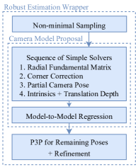
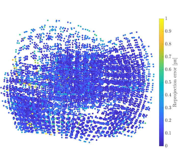
Figure 1: Method overview and result. (left) BabelCalib pipeline: the camera model proposal step ensures a good initialization, (right) example result showing residuals of reprojected corners of test images.

Camera calibration is a very non-linear task, hence a good initial guess is typically needed to obtain accurate parameters. Poor initial estimates are frequent source of failures. Sensible initial guesses are often available only for some of the model unknowns, e.g., initial values are often unavailable for parameters describing substantial lens distortions.

A second failure mode is caused by incorrect or grossly inaccurate measurements, e.g., corner detections, which are matched to fiducials on the calibration target. If corrupted data is used to estimate the initial guess, then the downstream model refinement will likely fail.

Our method addresses both failure modes. We introduce a solver that recovers all calibration parameters for a wide range of cameras (and lenses) such as pinhole, fisheye and catadioptric ones. We show that the proposed solver provides a good initialization for all critical intrinsics, which includes the center of projection and pixel aspect ratio. Our solver assumes only a planar calibration target. In addition, the initialization simultaneously improves the accuracy of corner detections while estimating the center of projection and camera pose by enforcing projective constraints. The solver is used within a RANSAC framework for efficient model generation. The model proposals are evaluated for consistency with the extracted features, and poorly extracted features and incorrect correspondences are rejected.

Our approach uses a back-projection model as an intermediate camera model. Back-projection models mapping image points to 3D ray directions are able to model a wide range of cameras (such as pinhole, fisheye and omni-directional cameras). Our approach (and therefore our main contribution) is to decouple the calibration task for general camera models into a much simpler calibration task for a powerful back-projection model followed by a regression task to obtain the parameters of the general target camera model. Effectively, we remove the need to generate a solver for each target camera model, which can be intractable, or result in solvers that are computationally expensive or numerically unstable in practice. Instead, we use an efficient solver for a back-projection model followed by an easier regression task to recover the target model parameters. The motivation for such an approach is given in Table 1, where it shows that projection equations are relatively simple once the radial component $R$ and the depth component $Z$ are known. These values are provided by the back-projection model. E.g., for the Kannala-Brandt model [20], estimation of its parameters is linear for given $R$ and $Z$.

Overall, our stratified approach to calibration circumvents many of the issues that are due to the highly non-linear behavior of many flexible camera models. BabelCalib performs both back-projection estimation and target model regression inside of a robust estimation framework, and directly returns the parameters of the target model. Fig. 1 illustrates the accuracy of our method for a fisheye lens on hold-out test images. The achieved high accuracy is spatially coherent across the entire calibration target over all test images.

1.1 Related Work

Camera calibration is an important tool in order to upgrade cameras from pure imaging devices to geometric sensors, and it has led to the development of many parametric models for cameras (and their lens systems) and the introduction of respective toolboxes (e.g. [8, 18, 43, 11, 38, 5, 26, 23, 32]). In order to facilitate the highest accuracy for the calibration parameters, a controlled, usually planar calibration target is employed in many applications. The use of dedicated images (“training data”) for the task of camera calibration distinguishes standard calibration from self-calibration, that extracts calibration parameters from uncontrolled “test” images (e.g. [9, 17, 30, 12, 42, 31, 24]).

Most relevant to our approach in terms of forward projection models are the unified camera model [13, 1, 26], the fisheye projection model by Kannala and Brandt [20], and the double sphere model [41]. Using these models for calibration tasks is not always straightforward and comes with their own set of assumptions.

E.g., the estimator proposed for the Double-Sphere model [41] requires that the circular field-of-view is visible to recover the center of projection and the aspect ratio, that the relative position of the spherical retinas be initialized, and that a non-radial line be identified to recover the focal length. Further, the method proposed for the popular Kannala-Brandt model requires specifying focal length and field of view [20].

The introduction of a linear solver to calibrate the division model in the back-projection framework [34] demonstrates the benefits of using back-projections. This linear method assumes known center of distortion and unit aspect ratio and is extended to a two-stage method in [35] to include estimation of the center of distortion. Urban et al. [40] identifies the shortcomings of this two-stage method and suggests joint refinement of all unknowns instead.

Finally, very general non-parametric models for cameras and lenses have been proposed (including [33, 15, 3, 36]), Our experiments indicate that appropriate parametric models are sufficient to model a wide range of cameras and lenses and are therefore—due to Occam’s razor—preferable in general.

2 Preliminaries

Let us define the camera matrix ${\mathtt{P}}$ mapping from scene coordinates to ray directions in the camera coordinate system as ${\mathtt{P}}=\operatorname{diag}(f,f,1)\begin{bmatrix}{\mathtt{R}}&\mathbf{t}\end{bmatrix}$, where $f$ is the focal length, ${\mathtt{R}}=\begin{bmatrix}\mathbf{r}_{1}&\mathbf{r}_{2}&\mathbf{r}_{3}\end{bmatrix}$ is the rotation matrix, and $\mathbf{t}=\begin{pmatrix}t_{x},&t_{y},&t_{z}\end{pmatrix}^{{\!\top}}$ is the translation vector. We build on the omni-directional camera model of Micusik and Pajdla [27], that relates the image point $\mathbf{u}=\begin{pmatrix}u,&v,&1\end{pmatrix}^{{\!\top}}$ and the scene point $\mathbf{X}$ as

$$\gamma g(\mathtt{A}\mathbf{u})={\mathtt{P}}\mathbf{X}\quad\text{s.t.}\quad\gamma>0.$$ (1)

In (1) the matrix $\mathtt{A}$ maps from image coordinates to sensor coordinates. Denote the center of projection as $\mathbf{e}=\begin{pmatrix}e_{x},&e_{y},&1\end{pmatrix}^{{\!\top}}$, the scale factor as $s$, and the pixel aspect ratio as $a$. For the initialization method we assume that the pixels are orthogonal, so we have

$$\mathtt{A}=\operatorname{diag}(a^{\mathsf{-1}},1,1)\operatorname{diag}(s^{\mathsf{-1}},s^{\mathsf{-1}},1)\mathtt{T}(-\mathbf{e}),$$ (2)

where $\mathtt{T}(\mathbf{x})$ is a homogeneous matrix encoding translation by $\mathbf{x}$. The nonlinear function $g(\cdot)\in\mathbb{R}^{3}\to\mathbb{R}^{3}$ in (1) maps from the retinal plane to ray directions in the camera coordinate system. For the initialization method, the typically small distortions caused by lens misalignment are ignored [16] so that we can model back-projection of $\mathbf{u}=\begin{pmatrix}u,&v,&1\end{pmatrix}^{{\!\top}}$ as radially symmetric, $g(\mathbf{u})=\begin{pmatrix}u,&v,&\psi(r(\mathbf{u}))\end{pmatrix}^{{\!\top}}$, where the radius of the retinal point is $r(\mathbf{u})=\sqrt{u^{2}+v^{2}}$.

Back-Projection with Division Model

We parameterize $\psi(\cdot)$ with the division model. It has a good ability to model significant lens distortions and was used in [34] for fisheye and catadioptric lenses with fields-of-view greater than $180^{\circ}$. The model is defined as

$$\psi(r)=1+\sum_{n=1}^{N}\lambda_{n}r^{2n}$$ (3)

Function $\psi(\cdot)$ is not invertible in general; however, we assume that there is only a single root $r^{*}\in[0,r^{\max}]$, where $r^{\max}$ is the image diagonal. More precisely, let $\mathbf{x}=\begin{pmatrix}x,&y,&w\end{pmatrix}^{{\!\top}}$ and let $h(\cdot)$ be the function projecting $\mathbf{x}$ to the retinal plane,

$$h(\mathbf{x})=\begin{pmatrix}\frac{r^{*}}{r(\mathbf{x})}x,&\frac{r^{*}}{r(\mathbf{x})}y,&1\end{pmatrix}^{\!\top},$$ (4)

where $r^{*}$ is the only solution of $\psi(r)=w$ in $[0,r^{\max}]$. Consequently,

$$\mathbf{u}=h(g(\mathbf{u})).$$ (5)

Multiple roots in $[0,r^{\max}]$ imply that a scene point maps to multiple image points, which is an implausible physical configuration.

Radial Fundamental Matrix

Without loss of generality, we assume the target to be on the plane $z=0$. Transforming a point $\mathbf{X}$ on the target to a ray direction in the camera coordinate system can be done by the homography $\mathtt{H}=\begin{bmatrix}\mathbf{r}_{1}&\mathbf{r}_{2}&\mathbf{t}\end{bmatrix}$ constructed from the camera matrix

$$\begin{split}{\mathtt{P}}\mathbf{X}&=\operatorname{diag}(f,f,1)\begin{bmatrix}{\mathtt{R}}&\mathbf{t}\end{bmatrix}\begin{pmatrix}X,&Y,&0,&1\end{pmatrix}^{{\!\top}}=\\ &\operatorname{diag}(f,f,1)\underbrace{\begin{bmatrix}\mathbf{r}_{1}&\mathbf{r}_{2}&\mathbf{t}\end{bmatrix}}_{\mathtt{H}}\underbrace{\begin{pmatrix}X,&Y,&1\end{pmatrix}^{{\!\top}}}_{\mathbf{x}}.\\ \end{split}$$ (6)

Hartley and Kang [15] used the radial fundamental matrix to recover the principal point of distorted pinhole cameras. We extend the radial fundamental matrix to recover the center of projection $\mathbf{e}$ and camera pose ${\mathtt{R}},\mathbf{t}$ for the back-projection model of [27]. We substitute $\operatorname{diag}(f,f,1)\mathtt{H}\mathbf{x}$ for $\mathtt{P}$$\mathbf{X}$ in (1) using (6), apply the projection function $h(\cdot)$ to both sides, and use (5) to eliminate $g$ giving

$$\begin{split}\mathbf{u}=\mathtt{A}^{\mathsf{-1}}h(1/\gamma\operatorname{diag}(f,f,1)\mathtt{H}\mathbf{x})=\\ {\mathtt{T}}(\mathbf{e})1/\gamma\operatorname{diag}(a(sfr^{*})/r(\mathbf{x}),(sfr^{*})/r(\mathbf{x}),1)\mathtt{H}\mathbf{x}.\end{split}$$ (7)

Note that the scaling by $(sfr^{*})/(\gamma r(\mathbf{x}))$ due to focal length, projection by $h(\cdot)$, pixel scale $s$ and depth multiplier $\gamma$ is entangled and acts radially. Substituting $\eta=(sfr^{*})/(\gamma r(\mathbf{x}))$ into (7) and crossing both sides with $\mathbf{e}$ gives

$$\begin{split}\left[{\mathbf{e}}\right]_{\times}\mathbf{u}&=\left[{\mathbf{e}}\right]_{\times}\mathtt{T}(\mathbf{e})\operatorname{diag}(a\eta,\eta,1/\gamma)\mathtt{H}\mathbf{x}\\ &=\left[{\mathbf{e}}\right]_{\times}\operatorname{diag}(a\eta,\eta,0)\mathtt{H}\mathbf{x}.\end{split}$$ (8)

The radial line $\left[{\mathbf{e}}\right]_{\times}\mathbf{u}$ is eliminated by taking the inner product of $\mathbf{u}$ with (8), and $\eta$ can be eliminated since it is non-zero. Denote the rows of $\mathtt{H}$ such that $\mathtt{H}=\begin{bmatrix}\mathbf{h}_{1}&\mathbf{h}_{2}&\mathbf{h}_{3}\end{bmatrix}^{\top}$. Then (8) simplifies to

$$0=\mathbf{u}^{\top}\left[{\mathbf{e}}\right]_{\times}\begin{pmatrix}a\mathbf{h}_{1}^{{\!\top}}\mathbf{x},&\mathbf{h}_{2}^{{\!\top}}\mathbf{x},&0\end{pmatrix}^{\top},$$

which can be rearranged to give the radial fundamental matrix $\mathtt{F}_{r}$ for omni-directional cameras

$$0=\mathbf{u}^{\top}\underbrace{\left[{\mathbf{e}}\right]_{\times}\begin{bmatrix}ar_{11}&ar_{12}&at_{x}\\ r_{21}&r_{22}&t_{y}\\ 0&0&0\end{bmatrix}}_{\mathtt{F}_{r}}\mathbf{x}.$$ (9)

The aspect ratio is modeled, but cannot be recovered without additional constraints. The radial fundamental matrix $\mathtt{F}_{r}$ is rank two by construction, and the center of projection $\mathbf{e}$ is a basis for the left null space of $\mathtt{F}_{r}$.

3 Obtaining the Initial Estimate

The methods proposed in this section ensure that a good initial guess of the camera model is made. The parameters are recovered by a sequence of simple solvers (see Fig. 1). The back-projection model of (1) corresponds image points to ray directions in the camera coordinate system. Given this correspondence, we show that regressing the commonly used projection models can be done easily. This enables the search for good initial guesses for the target projection model in a sampling framework, which increases the robustness of the method.

3.1 Solving the Radial Fundamental Matrix

The radial fundamental matrix is estimated to recover the center of projection and camera pose. The epipolar constraint on the radial fundamental matrix $\mathbf{u}^{\top}\mathtt{F}\mathbf{x}=0$ in (9) can be written as a linear constraint on $\mathtt{F}$

$$(\mathbf{x}\otimes\mathbf{u})^{\!\top}\operatorname{vec}(\mathtt{F})=0.$$ (10)

Following the classic solver for the fundamental matrix in [16], we use at least seven image-to-target point correspondences, denoted $\{\,\mathbf{u}_{i}\leftrightarrow\mathbf{x}_{i}\,\}$, to compute the null space of stacked constraints of the form (10). The nonlinear constraint $\det\mathtt{F}=0$ is enforced to recover at most three real solutions from the null space. The fundamental matrix consistent with the most correspondences is kept.

3.2 Solving the Center of Projection and Pose

As shown in (9), the center of projection is a basis for the left null space of $\mathtt{F}$

$$\zeta\mathbf{e}=\operatorname{null}{\mathtt{F}}^{\top}.$$ (11)

There is a scale ambiguity, denote it $\nu$, between the radial fundamental matrix $\mathtt{F}_{r}$ as formulated in (9) and the fundamental matrix $\mathtt{F}$ recovered by the seven-point method,

$$\mathtt{F}=\nu\mathtt{F}_{r}\quad\text{where }\mathtt{F}=\begin{pmatrix}f_{ij}\end{pmatrix}.$$ (12)

Let $r_{31},r_{32}$ be the unknown components of the rotation vectors $\mathbf{r}_{1}$ and $\mathbf{r}_{2}$. If we let $\mathtt{S}=\nu^{-1}\operatorname{diag}({a}^{-1},1,1)$, then $\mathbf{r}_{j}=\mathtt{S}\begin{pmatrix}f_{2j},&-f_{1j},&r_{3j}\end{pmatrix}^{\!\top}$. We use the orthonormality of $\mathbf{r}_{1}$ and $\mathbf{r}_{2}$ to put quadratic constraints on the unknowns,

$$\begin{split}&\|\mathtt{S}(f_{21},-f_{11},r_{31})^{\top}\|^{2}_{2}=\|\mathtt{S}(f_{22},-f_{12},r_{32})^{\top}\|^{2}_{2}\\ &\text{ and }\begin{pmatrix}f_{21},&-f_{11},&r_{31}\end{pmatrix}\mathtt{S}^{2}\begin{pmatrix}f_{22},&-f_{12},&r_{32}\end{pmatrix}^{\top}=0.\end{split}$$ (13)

There are four unknowns but only three constraint equations. Additional constraints are needed to recover the aspect ratio. The unknowns $\{\nu,a,r_{31},r_{32},t_{z},\lambda_{1},...,\lambda_{n}\}$ can be jointly recovered by solving a system of polynomial equations (see Sec. A in Supplemental); however, we chose to sample over the interval of aspect ratios $a\in[0.5,2]$ and recover $\{\nu,r_{31},r_{32}\}$ from (13).

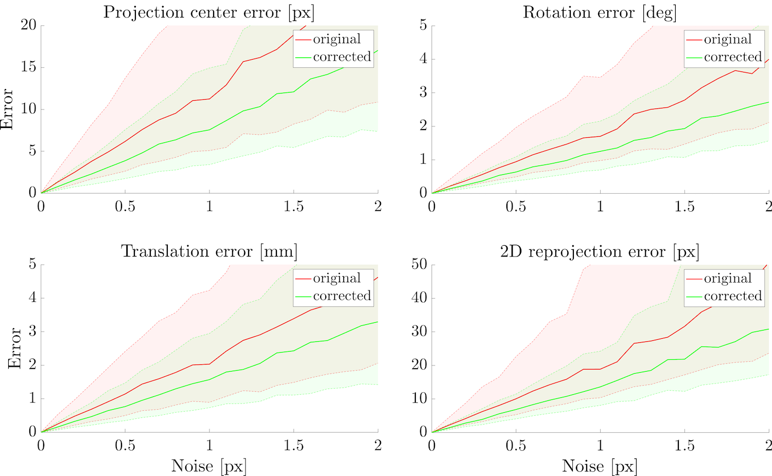
Figure 2: Correcting corners improves the initial guess. We evaluate the accuracy of the center of projection, camera pose and rewarped points using the original and corrected corners. Evaluation is done over 1000 experiments at each noise level. Solid curves are median errors, and shaded regions are interquartile ranges.

3.3 Corner Correction

Corner correction is defined such that given the radial fundamental matrix ${\mathtt{F}}_{r}$ and correspondence $\mathbf{u}_{i}\leftrightarrow\mathbf{x}_{i}$, the corrected corner is $\mathbf{u}_{i}^{*}=\mathbf{u}_{i}+\delta_{\mathbf{u}_{i}}$, where $\delta_{\mathbf{u}_{i}}$ is the smallest displacement such that $\mathbf{u}_{i}^{*}$ satisfies the epipolar constraint $\mathbf{u}_{i}^{*{\!\top}}{\mathtt{F}}_{r}\mathbf{x}_{i}=0$. The target fiducials $\{\,\mathbf{x}_{i}\,\}$ are assumed correct since they are noiseless. It can be shown [16] that the corrected corner $\mathbf{u}_{i}^{*}$ is recovered by projecting the measured corner $\mathbf{u}_{i}$ onto the epiline of $\mathbf{x}_{i}$,

$$\mathbf{u}_{i}^{*}=\mbox{proj}_{{\mathtt{F}}_{r}\mathbf{x}_{i}}(\mathbf{u}_{i}).$$ (14)

We refine the radial fundamental matrix ${\mathtt{F}}_{r}$ by minimizing the displacements with non-linear least squares. Eight correspondences are sufficient for correcting the sampled corners [16], but it is reasonable to use more since we expect a high inlier ratio for a calibration capture. The rank-two constraint is encoded with the parameterization ${\mathtt{F}}_{r}=\left[{\mathbf{e}}\right]_{\times}\begin{pmatrix}\mathbf{h}_{1}^{{\!\top}},&\mathbf{h}_{2}^{{\!\top}},&\mathbf{0}_{3}\end{pmatrix}^{\top}$. Then the refined fundamental matrix is recovered by solving

$$\mathbf{e}^{*},\mathbf{h}^{*}_{1},\mathbf{h}^{*}_{2}=\operatorname*{argmin}_{\mathbf{e},\mathbf{h}_{1},\mathbf{h}_{2}}\sum_{i}\delta_{\mathbf{u}_{i}}^{\top}\delta_{\mathbf{u}_{i}}$$ (15)

and reconstructing ${\mathtt{F}}^{*}_{r}$ from $\mathbf{e}^{*},\mathbf{h}^{*}_{1},\mathbf{h}^{*}_{2}$. The noisy detected corners are corrected according to (14) using ${\mathtt{F}}^{*}_{r}$.

Evaluation of Corrected Corners

Synthetic scenes were used to measure the accuracy gains to camera model estimation from corner correction. The camera was randomly posed to view a chessboard. Image resolution was $1200\times 800$ pixels, focal length $400$ pixels, and the center of projection was displaced to $\begin{pmatrix}700,&500\end{pmatrix}$. We added different levels white noise to the corners: $\sigma\in\{\,0,0.1,0.2,...,2\,\}$. Camera models were fit using either the original or corrected corners for 1000 images.

Clockwise from the top left, Fig. 2 reports (i) the distance between the estimated and ground truth center-of-projection, (ii) the smallest angle of rotation required to correct the estimated orientation, (iii) the distance between the estimated and ground-truth camera position, and (iv) the RMS reprojection error between an image grid and the reprojection of scene points by the estimated camera that should project onto the image grid . Fig. 2 shows that correcting corners reduces median errors of rotation, translation and RMS reprojection error by $31\%$, $28\%$, and $33\%$ on average.

3.4 Solving the Remaining Intrinsics and Depth

The homography ${\mathtt{H}}$ mapping from the camera coordinate system to coordinates of the retinal plane can be used to solve for the remaining parameters, $\gamma g({\mathtt{A}}\mathbf{u})=\operatorname{diag}(f,f,1){\mathtt{H}}\mathbf{x}.$ Note that $s$ and $f$ in ${\mathtt{A}}$ cannot be disentangled without additional knowledge about the camera such as the pixel size. Further, we assume that this information is unavailable, and let $f\leftarrow sf$. An unknown $\gamma$ is eliminated through the cross product,

$$g\left(\operatorname{diag}(f^{\mathsf{-1}},f^{\mathsf{-1}},1)\mathbf{u}^{\prime}\right)\times\begin{pmatrix}x^{\prime}\\ y^{\prime}\\ z^{\prime}+t_{z}\end{pmatrix}=0,$$ (16)

where $\mathbf{u}^{\prime}=\operatorname{diag}(a^{\mathsf{-1}},1,1)\mathtt{T}(-\mathbf{e})\mathbf{u}$, $x^{\prime}=\mathbf{h}_{1}^{\top}\mathbf{x}$, $y^{\prime}=\mathbf{h}_{2}^{\top}\mathbf{x}$, and $z^{\prime}=\begin{pmatrix}r_{31},&r_{32},&0\end{pmatrix}\mathbf{x}$. Reparameterizing $\tilde{\lambda}_{k}=\lambda_{k}/f^{2k-1}$ and collecting terms in (16) gives a system linear in the unknowns

$$\begin{bmatrix}&&\vdots\\ x_{i}^{\prime}&x_{i}^{\prime}{r_{i}^{\prime}}^{2}&...&x_{i}^{\prime}{r_{i}^{\prime}}^{2N}&-u_{i}^{\prime}\\ y_{i}^{\prime}&y_{i}^{\prime}{r_{i}^{\prime}}^{2}&...&y_{i}^{\prime}{r_{i}^{\prime}}^{2N}&-v_{i}^{\prime}\\ &&\vdots\\ \end{bmatrix}\begin{pmatrix}f\\ \tilde{\lambda}_{1}\\ \vdots\\ \tilde{\lambda}_{N}\\ t_{z}\end{pmatrix}=\begin{pmatrix}\vdots\\ u_{i}^{\prime}\cdot z_{i}^{\prime}\\ v_{i}^{\prime}\cdot z_{i}^{\prime}\\ \vdots\\ \end{pmatrix}$$ (17)

where $r_{i}^{\prime}=r(\mathbf{u}_{i}^{\prime})$ is the radius of the point $\mathbf{u}_{i}^{\prime}$.

Model Selection for the Division Model

The degree of division model $\psi(\cdot)$ defined in (3) needs to be chosen such that it can approximate the extreme radial profiles of fisheye and catadioptric rigs, and so that it does not overfit to noisy measurements for narrow field-of-view lenses. Clearly these are competing goals. We evaluated $\psi(\cdot)$ for polynomials of even degrees from two to ten. Model selection is performed on the dataset introduced in Sec. 5, which contains a wide range of lenses as well as catadioptric rigs.

The camera model of (1) is estimated linearly from sampled corner correspondences (denoted Initial in Table 2) as outlined above and fit with non-linear least squares (denoted Refined in Table 2) using all corners for each calibration capture. The weighted RMS reprojection error and inlier ratio are used to assess the accuracy of each model’s initial guess and refined solution across the entire dataset. Table 2 shows that models of degrees eight and ten significantly deviate from the optimal result, suggesting that they are over-fitting. The fourth-degree division model parameterized by $\{\,\lambda_{1},\lambda_{2}\,\}$ is the simplest model that is sufficiently flexible to provide a good initial guess. We estimate the back-projection function (1) using (3) with $N=2$.

Degree	Initial RMS [px],   inl. [%]	Refined RMS [px],   inl. [%]
2	5.342,    26.042	0.647,    97.086
4	4.585,    28.991	0.587,    97.403
6	4.516,    26.184	0.587,    97.399
8	7.429,    13.307	1.020,    93.660
10	12.804,       8.448	4.812,    61.267

Table 2: Model selection for the division model. A polynomial of degree four gives the best results overall.

Model-to-Model Regression

A radial projection function, denoted $\phi_{\theta}(R,Z)$, can always be parameterized by how it maps a point at radius $R$ from the optical axis and depth $Z$ from the principal plane to the retinal plane (see Table 1). This parameterization admits a universal way to regress radially-symmetric projection functions against the division model.

If the user-selected projection model does not have the division model for its radial profile, then the following optimization must be performed

$$\sum_{k}(\phi_{\theta}(r_{k},\psi(r_{k}))-r_{k})^{2}\rightarrow\min_{\theta},\vspace{-7pt}$$ (18)

where radii $r_{k}=\frac{k-1}{K-1}r^{\max}$ are uniformly sampled from zero to the maximum radius $r^{\max}$. All regressions for the forward models in Table 1 are either linear (BC, KB, UCM, EUCM) or easy to perform with the least squares (FOV, DS). See Sec. B in Supplemental for the details and example of regression against the Kannala-Brandt model.

OV-Plane—130108MP,   $0.478$ px RMS	OV-Corner—Cam4,   $0.770$ px RMS	OV-Cube—Cam1,   $0.268$ px RMS

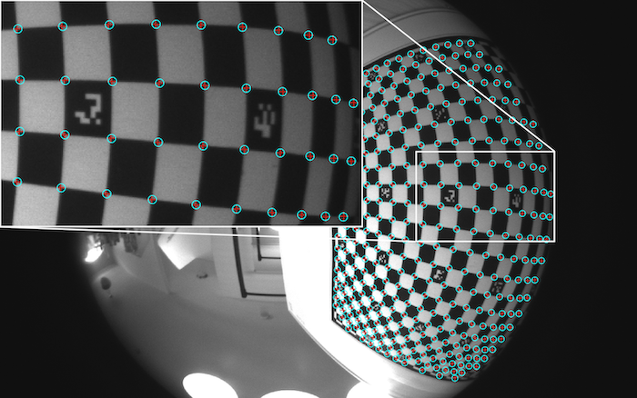
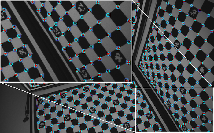
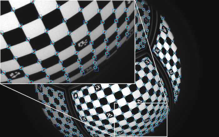
Figure 3: Projection of calibration target from estimated calibration. Detected corners are red crosses, target projected using initial calibration are blue squares and using the final calibration are cyan circles.

4 Robust Estimation Framework

In this section we propose a calibration framework that is robust to corner detection errors, works with either one or multiple calibration boards, and handles the partial visibility of board fiducials across the calibration capture. The robustness of the method is, in part, achieved using the camera geometry estimators proposed in Sec. 3. With these estimators, an accurate estimate of any of the board models listed in Table 1 can be recovered from a sample of noisy corner detections. However, corner extraction can fail due to the detector’s inability to localize highly-distorted saddle points [14]. The grid search can also fail at the extents of a fisheye image because of highly-distorted neighborhoods. Occlusions can also create false corners. We incorporate the solvers of Sec. 3 into a RANSAC-based framework to handle bad detections [10]. The method fits camera models sampled from corner-to-board correspondences. The models are scored with a robust objective. During sampling, the best-so-far model is kept and refined with a maximum-likelihood estimator, which is inspired by the local optimization step in [4]. The output of the model is a maximum-likelihood fit of camera intrinsics and extrinsics. The estimators proposed in Sec. 3 are very simple, so they are fast and are well-suited for use in the model proposal step of RANSAC. Algorithm 1 in Sec. C of Supplemental may be helpful as a cross-reference for the next paragraphs that specify the method.

The input to the method is a set of 2D-3D correspondences that match corner detections with board fiducials, which we denote $\mathbf{X}_{ij}\leftrightarrow\mathbf{u}_{ijk}$. Indices $i$ and $j$ indicate a particular fiducial $i$ on plane $j$, and $k$ indicates the image of the corner detection $\mathbf{u}_{ijk}$ of fiducial $\mathbf{X}_{ij}$. For each RANSAC iteration, we sample an image $k$, a plane $j$ visible in image $k$, and a non-minimal sample of $14$ correspondences that are used to compute the radial fundamental matrix, center of projection, and corner correction according to (10), (11), and (14). The utilized sample size of $14$ correspondences was cross-validated.

Dataset	# cam., # img.	DFOV range	Max. img. size
Kalibr	$8$,  $140+60$	$110^{\circ}$—$268^{\circ}$	$1680\times 1680$
OCamCalib	$9$,  $\,\,\,79+40$	$130^{\circ}$—$266^{\circ}$	$3840\times 2880$
UZH-DAVIS	$4$,  $140+60$	$124^{\circ}$—$148^{\circ}$	$346\times 260$
UZH-Snapdragon	$4$,  $140+60$	$144^{\circ}$—$166^{\circ}$	$640\times 480$
OV-Corner	$8$,  $280+120$	$109^{\circ}$—$109^{\circ}$	$1280\times 800$
OV-Cube	$4$,  $105+49$	$159^{\circ}$—$183^{\circ}$	$1280\times 800$
OV-Plane	$4$,  $\,\,\,92+41$	$88^{\circ}$—$187^{\circ}$	$1280\times 800$

Table 3: Calibration dataset details. Train-test split of the images is indicated by $+$. The diagonal field of view (DFOV) is approximated using intrinsic calibration.

The aspect ratio is a necessary parameter for the pose and intrinsics estimators. If the camera has non-square pixels or an anamorphic lens, we sample an aspect ratio from the interval $[0.5,2]$. Pose and intrinsics are estimated as derived in (13) and (17). The radial profile of the user-selected camera model is regressed against the radial profile of the division model using (18), if the division model is not the desired model. The model-to-model regression generates the camera geometry portion of the RANSAC model proposal. Given the estimate of intrinsics, the poses for the remaining images are computed using P3P (Perspective-3-Point [28]) from three sampled corner-to-board correspondences. The camera poses are added to the intrinsics to give a RANSAC model proposal.

	OpenCV-BC	Kalibr-BC	Ours-BC
	RMS [px],   inl. [%]
Cam0	0.886,   90.9	0.945,   87.3	0.704,   96.1
Cam1	0.781,   95.2	0.893,   88.8	0.674,   98.0
Cam2	0.773,   96.1	0.756,   95.6	0.720,   96.9
Cam3	0.733,   97.0	0.953,   87.6	0.710,   96.4
Cam4	0.757,   97.3	0.828,   93.6	0.679,   97.6
Cam5	0.772,   96.4	0.831,   91.7	0.759,   96.0
Cam6	0.715,    95.4	0.748,   94.5	0.677,   96.0
Cam7	0.701,   96.6	0.855,   90.6	0.641,   97.5

Table 4: Pose evaluation for the BC model. OV-Corner test images used.

	OpenCV-KB	Kalibr-KB	Ours-KB	OpenCV-UCM	Kalibr-UCM	Ours-UCM
	RMS [px],   inl. [%],   # failures
OV-Corner	0.746,   94.4,   0/8	0.882, 90.3,   0/8	0.695,   96.8,   0/8	1.187,   75.4,   0/8	0.953,   88.8,   0/8	0.812,   94.8,   0/8
OV-Cube	FAIL,   4/4	0.411, 92.7,   2/4	0.265,   97.5,   0/4	0.493,   86.7   0/4	0.440,   90.8   0/4	0.316,   96.8,   0/4
OV-Plane	2.449,   70.2,   0/4	0.658, 92.9,   1/4	0.596,   94.0,   0/4	0.854,   80.7,   0/4	0.669,   90.6,   0/4	0.606,   93.6,   0/4
Kalibr	2.291,   53.9,   3/8	0.194, 99.8,   3/8	0.173,   99.9,   0/8	0.355,   95.2,   0/8	0.350,   94.6,   0/8	0.326,   97.1,   0/8
OCamCalib	2.921,   67.0,   3/9	0.696, 97.2,   4/9	0.676,   97.3,   0/9	0.782,   93.4,   2/9	0.776,   94.6,   0/9	0.784,   97.2,   0/9
UZH-DAVIS	0.389,   96.3,   0/4	0.389, 96.3,   0/4	0.382,   96.3,   0/4	0.503,   95.3,   0/4	0.490,   93.2,   0/4	0.385,   96.2,   0/4
UZH-Snapdragon	0.265,   99.6,   0/4	0.268, 99.6,   0/4	0.254,   99.6,   0/4	0.517,   97.3,   0/4	0.299,   99.4,   0/4	0.286,   99.5,   0/4
	Kalibr-FOV	Ours-FOV	Kalibr-EUCM	Ours-EUCM	Kalibr-DS	Ours-DS
	RMS [px],   inl. [%],   # failures
OV-Corner	0.931,   88.7,   0/8	0.743,   96.1,   0/8	FAIL,   8/8	0.751,   95.8,   0/8	0.967,   88.5,   0/8	0.812,   94.5,   0/8
OV-Cube	FAIL    4/4	1.356,   19.3,   0/4	0.416,   91.9,   3/4	0.273,   97.0,   0/4	0.413,   92.7,   0/4	0.269,   97.3,   0/4
OV-Plane	0.867,   83.1,   1/4	0.863,   82.8,   0/4	0.584,   96.8,   2/4	0.542,   96.6,   0/4	0.644,   93.2,   0/4	0.606,   93.6,   0/4
Kalibr	0.257,   99.1,   3/8	0.237,   99.2,   0/8	0.250,   98.9,   0/8	0.230,   99.2,   0/8	0.264,   98.2,   0/8	0.326,   97.1,   0/8
OCamCalib	0.786,   96.1,   4/9	0.779,   96.2,   0/9	0.580,   97.8,   6/9	0.561,   97.7,   0/9	0.755,   94.6,   0/9	0.739,   97.7,   0/9
UZH-DAVIS	0.421,   95.5,   1/4	0.417,   95.7,   0/4	0.415,   95.6,   1/4	0.411,   95.6,   0/4	0.393,   96.2,   0/4	0.382,   96.2,   0/4
UZH-Snapdragon	0.250,   99.6,   1/4	0.234,   99.6,   0/4	0.246,   99.6,   1/4	0.232,   99.6,   0/4	0.284,   99.3,   0/4	0.286,   99.5,   0/4

Table 5: Pose Evaluation for fisheye and catadioptric rigs. Estimated models are (top) KB, UCM, and (bottom) FOV, EUCM, and DS. Each method’s performance on a dataset is given by the weighted RMS reprojection error [px], the inlier ratio [%], and the number of catastrophic failures.

The reprojection error is evaluated against the entire calibration capture with the robust objective

$$\mathcal{J}(\Theta)=\sum_{ijk}\rho(d(\pi\left(\begin{bmatrix}{\mathtt{R}}_{jk}&\mathbf{t}_{jk}\end{bmatrix}\mathbf{X}_{ij}),~{}\mathbf{u}_{ijk})\right),$$ (19)

where $\pi(\cdot)$ is the selected projection function, $d(\cdot,\cdot)$ is the Euclidean distance, $\rho(\cdot)$ is the the Huber loss function [19], and $\Theta=\{\theta,{\mathtt{K}},{\mathtt{R}}_{jk},\mathbf{t}_{jk}\}$ are the calibration parameters. In the case of multiple planar targets, the poses ${\mathtt{R}}_{jk},\mathbf{t}_{jk}$ are constructed using the absolute poses of the cameras, ${\mathtt{R}}^{c}_{k},\mathbf{t}^{c}_{k}$, and the relative poses of the boards with respect to the reference board, ${\mathtt{R}}^{b}_{j},\mathbf{t}^{b}_{j}$,

$${\mathtt{R}}_{jk}={\mathtt{R}}^{c}_{k}{\mathtt{R}}^{b}_{j}\qquad\mathbf{t}_{jk}={\mathtt{R}}^{c}_{k}\mathbf{t}^{b}_{j}+\mathbf{t}^{c}_{k}.$$

If RANSAC encounters a best-so-far calibration proposal, then the model refinement step, $\mathcal{J}(\Theta)\to\min_{\Theta}$, is invoked. The axis-angle representation is used to minimally parameterize the rotations for the bundle adjustment. Proposals are ranked by their inlier ratio, and the inlier ratio is computed according to

$$\mathcal{I}(\Theta)=\frac{1}{M}\sum_{ijk}1_{\{\leq\tau\}}\left(d\left(\pi\left(\begin{bmatrix}{\mathtt{R}}_{jk}~{}\mathbf{t}_{jk}\end{bmatrix}\mathbf{X}_{ij}\right),\mathbf{u}_{ijk}\right)\right),$$ (20)

where $M$ is the total number of image-to-target correspondences, $1_{A}\left(\cdot\right)$ is an indicator function, and $\tau$ is the scale of the robust estimator.

5 Evaluation

The benchmark surveys a wide variety of lens types and includes catadioptric rigs. We aggregate several established datasets that are commonly used for testing the accuracy of camera calibration frameworks: (i) Double Sphere [41], (ii) EuRoC [2], (iii) TUM VI [37], (iv) and ENTANIYA  . We call the aggregated dataset Kalibr since the Kalibr calibration framework [25] was used in the original publications cited above. Kalibr has eight cameras, most of which are fisheyes. We also test the OCamCalib [34] dataset, which has five fisheye lenses and four catadioptric rigs; and the UZH [6] dataset, which consists of eight wide-angle and fisheye cameras captured from a drone. The dataset is split into two subsets, DAVIS and Snapdragon.

We also acquired calibration data from sixteen OmniVision cameras fitted with different lenses giving fields of view ranging from $88^{\circ}$ to $187^{\circ}$. The cameras were calibrated using three different targets containing AprilTags [29]: Plane, Corner and Cube, with one, three, and four chessboards, respectively (see Fig. 3). The OmniVision capture is denoted OV. The specifications of the cameras from each dataset are listed in Table 3.

	OCamCalib-DIV	Ours-DIV
	RMS [px],   inl. [%]
Fisheye1	0.631,   98.3	0.603,   97.1
Fisheye190deg	0.642,   96.8	0.621,   95.2
Fisheye2	0.480,   97.9	0.458,   97.9
GOPRO	1.097,   95.3	1.177,   96.9
KaidanOmni	0.595,   100	0.574,   98.3
Ladybug	0.661,   98.8	0.658,   97.5
MiniOmni	0.795,   97.7	0.712,   95.6
Omni	0.828,   93.3	0.836,   97.1
VMRImage	0.560,   100	0.560,   99.2

Table 6: Pose evaluation for the DIV model. The test images from OCamCalib were used.

We evaluated state-of-the-art camera calibration frameworks that support the projection models listed in Table 1. OpenCV supports three models: BC [8], KB [20], and UCM [26, 23]. In addition to those models, the Kalibr framework [25] supports the FOV [7], EUCM [21] and DS [41] models. The OCamCalib (MATLAB) framework for fisheye and catadioptric rigs has the DIV [34, 40] model.

BabelCalib can regress all the camera models listed in Table 1. We compare each state-of-the-art calibration method over their supported models with the BabelCalib estimation of the same models. The state of the art was provided with a reasonable initial guess for the focal length, and the center of projection was initialized to the image center. The proposed BabelCalib does not require, nor was it given, a user-provided initial guess.

Original	Displaced	Non-Square	Displaced + Non-Square

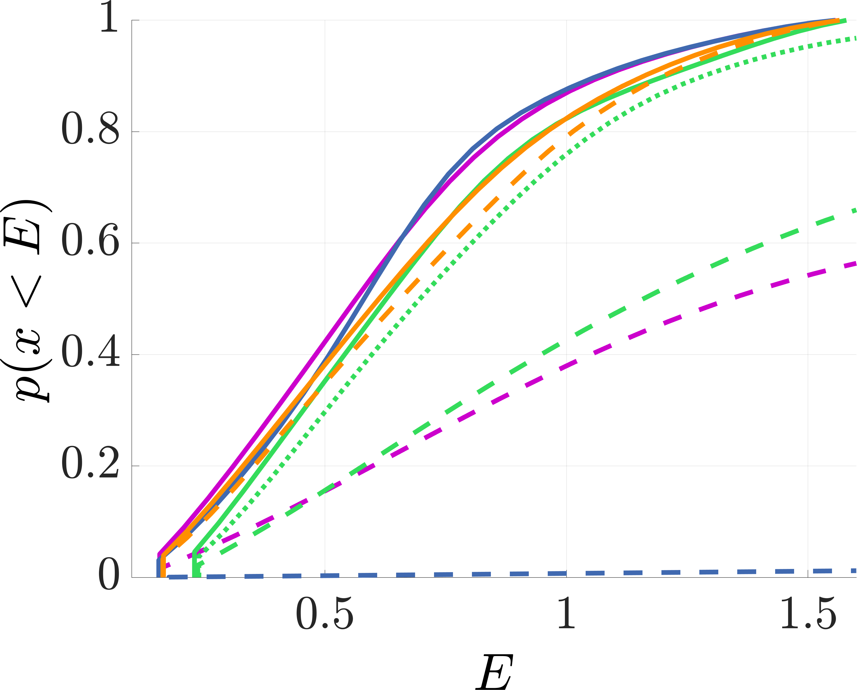
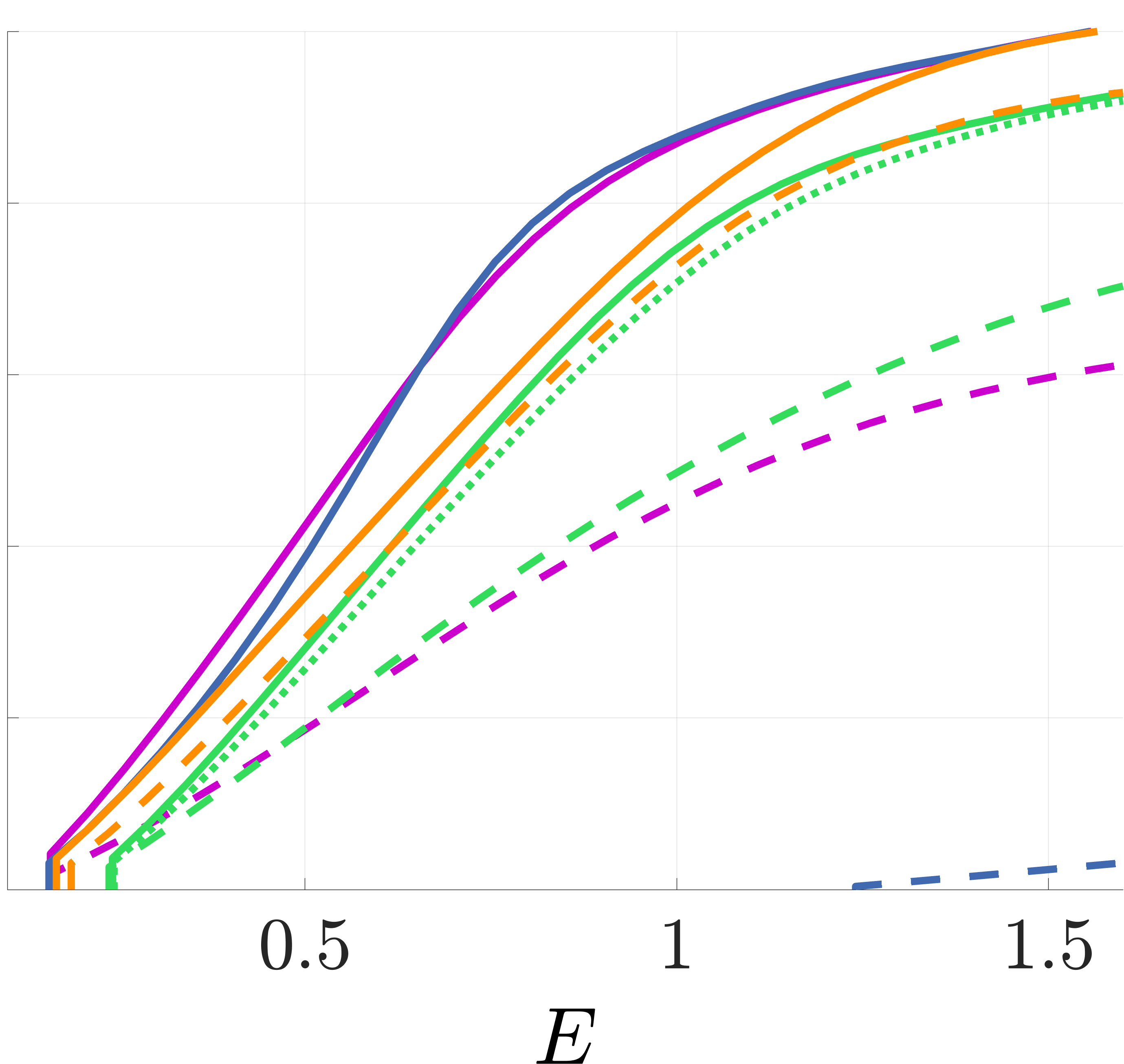
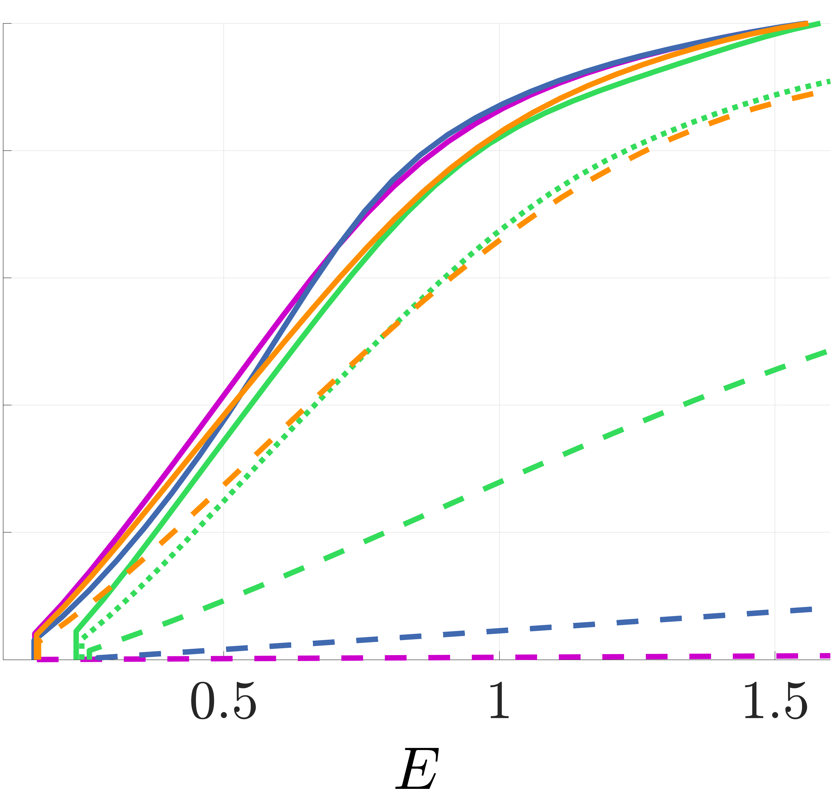
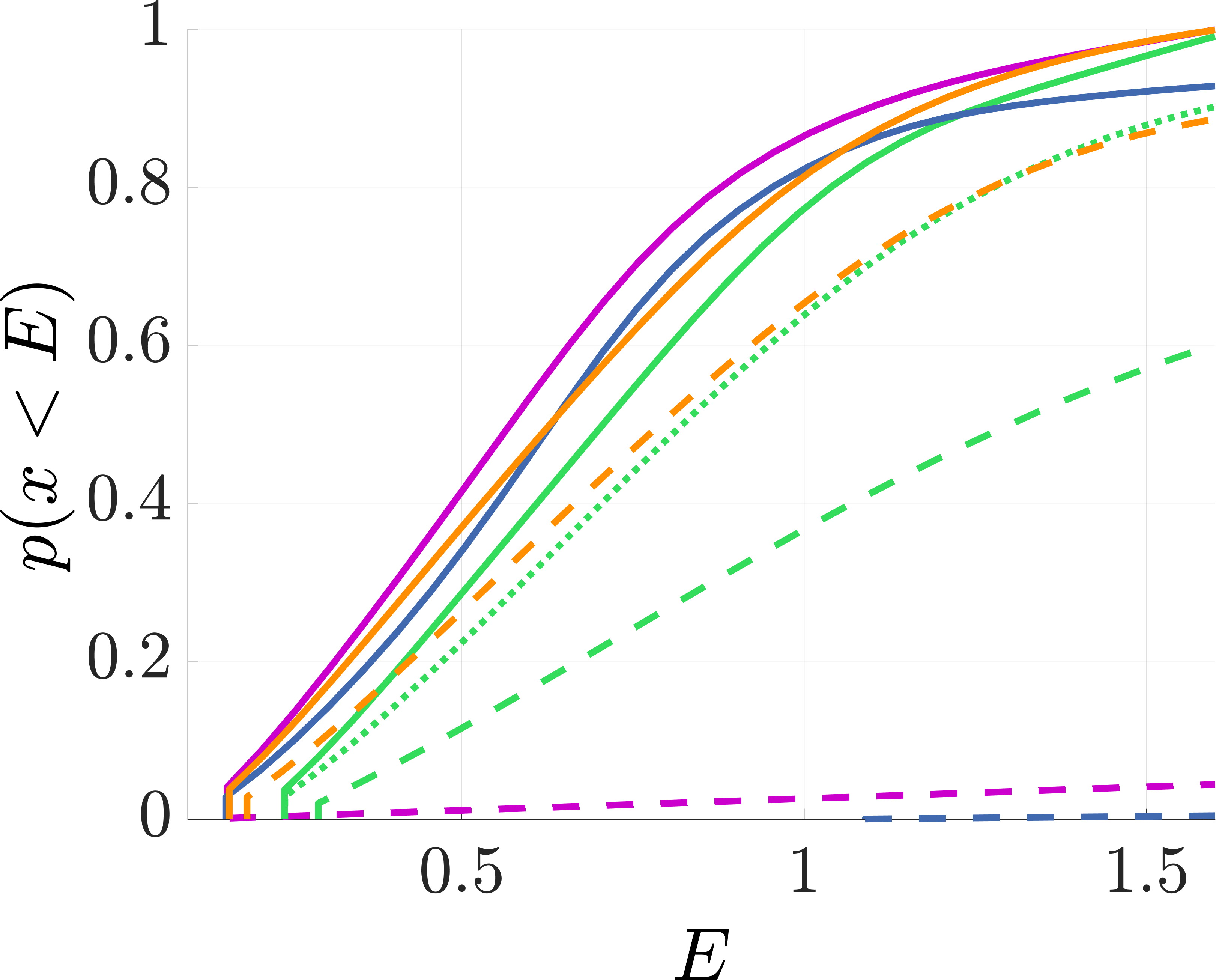
Figure 4: Performance summary for all calibration captures. The empirical CDFs show the relative performance of each method across all calibration datasets. The methods are tested for different augmentation types. The probability that the weighted RMS reprojection error is less than $E$ is plotted. The weighted RMS reprojection error is normalized to correspond to a $1000\times 1000$ px image. BabelCalib performs better for every model type on the original and augmented imagery.

5.1 Camera Pose Estimation

Pose accuracy for held-out test images from the calibration captures is used to evaluate the calibration of each method. Camera intrinsics are fixed to the calibration, and the objective $\mathcal{J}(\Theta)$ of (19) is minimized over camera poses only. The train-test split for each dataset is specified in Table 3. Pose accuracy is measured by the robust RMS reprojection error of (19) and the mean inlier ratio evaluated by (20). The error and inlier ratio for each dataset are averaged across the cameras where the method returns a model. This policy favors the state of the art since BabelCalib returns models for all cameras. These measures are reported for each framework-dataset combination in the comparison tables. The winner is boldfaced. A tie is declared if a method is not best on both measures. In this, we mark the highest number of failures in red.

OpenCV-BC	8.76%	Kalibr-BC	17.68%
OpenCV-KB	42.96%	Kalibr-KB	12.41%
OpenCV-UCM	24.66%	Kalibr-UCM	12.00%
Kalibr-FOV	6.11%	Kalibr-EUCM	9.92%
OCamCalib-DIV	2.05%	Kalibr-DS	5.36%

Table 7: Accuracy gains with respect to model type. BabelCalib regressions significantly reduce the weighted RMS reprojection error for all camera model types with respect to the estimates provided by the tested frameworks.

Table 4 reports results for the narrow-medium FOV lenses in the OV-Corner dataset. We breakout the results for each camera. The suitable model for this lens type is a pinhole projection with additive BC distortion. BabelCalib outperforms OpenCV and Kalibr. Table 5 reports results for fisheye lenses and catadioptric rigs. Kalibr and OpenCV have both a 24% failure rate for the Kannala-Brandt model, and Kalibr has a 34% failure rate for FOV and 51% failure rate for EUCM. In contrast, BabelCalib has no calibration failures. BabelCalib consistently gives the best results for each model type, even after discarding catastrophic failures for the state-of-the-art.

Table 6 reports calibrations using the DIV model on the OCamCalib dataset. OCamCalib-DIV is evaluated only on OCamCalib since it requires all fiducials to be visible across the capture. OCamCalib is the only dataset where this holds. BabelCalib and OCamCalib give comparable results. This dataset includes catadioptric rigs, which shows the flexibility of BabelCalib.

Table 7 summarizes the mean reduction of RMS weighted reprojection error for each dataset-model combination realized by BabelCalib over the state of art. BabelCalib gives a significant error reduction for all framework-model combinations, even after discarding the calibration failures of the state of the art. See Fig. C.2 in Supplemental for more qualitative results and also Sec. D which evaluates calibration performance from a limited amount of images.

Displaced Center and Non-Square Pixels

We augmented the datasets by adding cropped or stretched images to simulate a displaced projection center or a CCD with rectangular pixels. Displacement was $\begin{pmatrix}0.15w,0.15h\end{pmatrix}$ pixels for a $w\times h$ image, and pixel aspect ratio was 1.33:1. Fig. 4 reports the distributions of robust RMS reprojection errors for pose estimation on test images for the original and augmented data. Several model-framework combinations are evaluated. For comparison, the errors are normalized to correspond to a $1000\times 1000$ pixel image. BabelCalib finds a higher percentage of accurate calibrations on the original and augmented data for all models.

6 Conclusion

BabelCalib recovers significantly more accurate calibrations than three widely used frameworks and suffers no catastrophic failures. BabelCalib maintains its dominance for all commonly used models on a large survey of cameras with narrow, wide-angle and fisheye lenses, as well as catadioptric rigs. BabelCalib maintains its performance for cameras with displaced center of projections or non-square pixels. It doesn’t require model initialization nor hyper-parameter tuning, so it’s easy to use. Moreover, the regression framework easily admits additional camera models.

Acknowledgments

Y. Lochman, C. Zach and J. Pritts were partially supported by the Wallenberg AI, Autonomous Systems and Software Program (WASP) funded by the Knut and Alice Wallenberg Foundation.

BabelCalib: A Universal Approach to Calibrating Central Cameras
Supplemental Material

A Aspect Ratio Solver

The epipolar constraint $\mathbf{u}^{\top}{\mathtt{F}}\mathbf{x}=0$ is invariant to a projective change of coordinates. This implies that the aspect ratio cannot be recovered using only the constraints available from the radial fundamental matrix (e.g., see (13)). Additional constraints can be obtained by enforcing the concurrence of back-projected corners with their corresponding scene points using (1). The constraints given by (1) generate polynomial equations of the unknown aspect ratio, remaining unknowns of ${\mathtt{H}}$, and the unknown division model parameters $\{a,h_{31},h_{32},h_{33},\lambda_{1},...,\lambda_{n}\}$. The formulation introduces $N+1$ unknowns, but the formulation is invariant to the scale of ${\mathtt{H}}$. The minimal solution requires $N/2+2$ image-to-target correspondences.

Let $\mathbf{u}^{\prime}$ be the projection center-subtracted image point $\mathbf{u}^{\prime}=\mathtt{T}(-\mathbf{e})\mathbf{u}$. Then we can rewrite (1) as following

$$\begin{pmatrix}u^{\prime}/f\\ v^{\prime}/f\\ \psi(r(\operatorname{diag}(a^{-1},1,1)\mathbf{u}^{\prime}))\end{pmatrix}\times\underbrace{\operatorname{diag}(a,1,1){\mathtt{H}}}_{\hat{\mathtt{H}}}\mathbf{x}=\mathbf{0}.$$ (21)

Solving (10) and (11) gives the radial fundamental matrix ${\mathtt{F}}$ and projection center $\mathbf{e}$, respectively. We use the relation ${\mathtt{F}}\sim\left[{\mathbf{e}}\right]_{\times}\begin{pmatrix}a\mathbf{h}_{1}^{\top}\mathbf{x},&\mathbf{h}_{2}^{\top}\mathbf{x},&0\end{pmatrix}^{\top}$ to determine the first two rows of the matrix $\hat{\mathtt{H}}$, up to scale, $\hat{}\mathbf{h}_{1}^{\top}=\begin{pmatrix}f_{21},&f_{22},&f_{23}\end{pmatrix}$ and $\hat{}\mathbf{h}_{2}^{\top}=-\begin{pmatrix}f_{11},&f_{12},&f_{13}\end{pmatrix}$.

Rewriting (21) in terms of the unknowns gives

$$\begin{pmatrix}u^{\prime}\\ v^{\prime}\\ f\left(1+\sum_{n=1}^{N}\lambda_{n}r_{0}(a)^{2n}\right)\end{pmatrix}\times\begin{pmatrix}x^{\prime}\\ y^{\prime}\\ \hat{\mathbf{h}}_{3}^{\top}\mathbf{x}\end{pmatrix}=0,$$ (22)

where $r_{0}(a)=\sqrt{(\frac{u^{\prime}}{a})^{2}+{(v^{\prime})}^{2}}$,  $x^{\prime}=\hat{}\mathbf{h}_{1}^{\top}\mathbf{x}$,  $y^{\prime}=\hat{}\mathbf{h}_{2}^{\top}\mathbf{x}$. After reparameterizing with $b=a^{2}$, it can be seen that for $N=1$, (22) is linear in the unknowns and for $N=2$, a polynomial system of degree three must be solved.

We tested the solvers for the cases $N=1$ and $N=2$ on synthetic data and found that they are sensitive to noise. With a sufficiently good guess on aspect ratio, the solver in (17) performs better than the aspect ratio solver (see Fig. C.1). We opted to sample over aspect ratio rather than introduce these solvers. We leave the incorporation of minimal solvers for unknown aspect ratio for future work.

B Recovering Radial-Projection Functions for User-Selected Camera Models

The detected corners $\mathbf{u}$ can be back-projected to rays $\gamma g(\mathbf{u})=\gamma\begin{pmatrix}u,&v,&\psi(r(\mathbf{u}))\end{pmatrix}^{{\!\top}},\gamma>0$ in the direction of the board fiducials in the camera’s coordinate system. The polar angle of the ray determines how the points of the ray are projected, so any point of the ray can be used (equivalently, any $\gamma>0$ in (1) can be used). The distances to the optical axis $R$ and principal plane $Z$ are computed from the unit vector concurrent with the ray, $\frac{g(\mathbf{u})}{\|g(\mathbf{u})\|}$. With the radii and depths recovered, least squares can be used to recover the unknowns of the radial projection functions listed in Tables 1. This demonstrates the ease with which BabelCalib is extended.

Division Model to Kannala-Brandt Regression

The experiments of Sec. 5 confirm that the Kannala-Brandt (KB) model is the most flexible and accurate over the largest range of lenses, which is consistent with the results of [41]. We also found that the Kannala-Brandt model is also effective for catadioptric rigs (see Table 5).

The number of failed calibrations of OpenCV and Kalibr reported in Table 5 suggests that Kannala-Brandt is one of the hardest camera models to initialize. Directly computing a model proposal for Kannala-Brandt is difficult. The displacement of the projection from the optical center is proportional to a polynomial function of $\operatorname{atan2}$. The trigonometric function $\operatorname{atan2}$ is not easily eliminated since the unknown depth $Z$ is unique to each fiducial on the chessboard. Thus the problem cannot be solved as a polynomial system. BabelCalib initializes Kannala-Brandt by linearly regressing its parameters against the estimated division model, which is formulated in Sec. 3. We derive the linear system here to show how easy the model-to-model regression is once the back-projection function is known.

We back-project the corners $\mathbf{u}_{i}=\begin{pmatrix}u_{i},&v_{i},&1\end{pmatrix}^{\top}$ to ray directions $\mathbf{x}_{i}^{\prime}=\begin{pmatrix}x^{\prime}_{i},&y^{\prime}_{i},&z^{\prime}_{i}\end{pmatrix}^{\top}$ where $\mathbf{x}_{i}^{\prime}=g({\mathtt{K}}^{-1}\mathbf{u}_{i})$. The radii and depths are computed as $R_{i}=\sqrt{x^{\prime 2}_{i}+y^{\prime 2}_{i}}$ and $Z_{i}=z^{\prime}_{i}$, respectively. The polar angles $\omega_{i}=\operatorname{atan2}{(R_{i},Z_{i})}$ are determined, and the unknown coefficients of the polynomial $r_{i}=\omega_{i}+\sum^{4}_{n=1}k_{n}\omega_{i}^{2n+1}$ can be determined linearly,

$$\vspace{-20pt}\begin{bmatrix}&\vdots&\\ \omega_{i}^{3}&\ldots&\omega_{i}^{9}\\ \omega_{i+1}^{3}&\ldots&\omega_{i+1}^{9}\\ &\vdots&\\ \end{bmatrix}\begin{pmatrix}k_{1}\\ k_{2}\\ k_{3}\\ k_{4}\end{pmatrix}=\begin{pmatrix}\vdots\\ r_{i}-\omega_{i}\\ r_{i+1}-\omega_{i+1}\\ \vdots\end{pmatrix}.\vspace{20pt}$$ (23)

Solving (23) fully specifies the Kannala-Brandt projection model since the center of projection $\mathbf{e}$ and the focal length $f$ are known from estimation of the back-projection model — from (11) and (17), respectively.

C Algorithm

To summarize the proposed RANSAC-based calibration framework detailed in Sec. 4, we provide Algorithm 1 with all the crucial steps of the BabelCalib framework. The details on the pose optimization are omitted in the algorithm.

Input: 2D-3D point correspondences $\mathbf{u}_{ijk}\leftrightarrow\mathbf{X}_{ij}$

Parameters: Radial projection model $\phi_{\theta}$

Output: $\Theta^{\text{*}}=\{\theta^{\text{*}},{\mathtt{K}}^{\text{*}},{\mathtt{R}}_{jk}^{\text{*}},\mathbf{t}_{jk}^{\text{*}}\}$

$\mathcal{J}_{0}^{\text{*}}\leftarrow\infty,\,\,\mathcal{J}^{\text{*}}\leftarrow\infty$

repeat

      Sample image $k^{\prime}$ and plane $j^{\prime}$

      Sample $\{\mathbf{u}_{ij^{\prime}k^{\prime}}\leftrightarrow\mathbf{X}_{ij^{\prime}}\}_{i=1}^{N}$

      Compute $\mathbf{e}$ and $\mathtt{F}$ from $\{\mathbf{u}_{ij^{\prime}k^{\prime}}\leftrightarrow\mathbf{X}_{ij^{\prime}}\}_{i=1}^{N}$ with (15)

      Correct corners $\mathbf{u}_{ij^{\prime}k^{\prime}}$ to $\mathbf{u}^{*}_{ij^{\prime}k^{\prime}}$ with (14)

      Compute $\{{\mathtt{R}}_{j^{\prime}k^{\prime}},t_{x},t_{y}\}$ from ${\mathtt{F}}$ with (13)

      Sample aspect ratio $a$ from $[0.5,2]$

      Compute $\{f,\lambda_{1},...,\lambda_{N},t_{z}\}$ with (17)

      ${\mathtt{K}}\leftarrow{\mathtt{T}}(\mathbf{e})\operatorname{diag}(af,f,1),\,\,\mathbf{t}_{j^{\prime}k^{\prime}}\leftarrow\begin{pmatrix}t_{x},&t_{y},&t_{z}\end{pmatrix}^{\top}$

      if $\phi^{-1}_{\theta}$ is not the division model then

           Regress $\theta$ of $\phi_{\theta}$ with (18)

          

           end if

          for $(k,j)\neq(k^{\prime},j^{\prime})$ do

                Sample image $k$ and plane $j$

                Back-project the corners $\mathbf{x}_{ijk}^{\prime}\leftarrow g({\mathtt{K}}^{-1}\mathbf{u}_{ijk})$

                Compute $\{{\mathtt{R}}_{jk}$, $\mathbf{t}_{jk}\}$ from $\{\mathbf{x}_{ijk}^{\prime}\}_{i}$ with [28]

               

                end for

               $\Theta_{0}\leftarrow\{\theta,{\mathtt{K}},{\mathtt{R}}_{jk},\mathbf{t}_{jk}\}$

                Compute loss $\mathcal{J}_{0}\leftarrow\mathcal{J}(\Theta_{0})$ with (19)

                if $\mathcal{J}_{0}<\mathcal{J}_{0}^{*}$ then

                     $\mathcal{J}_{0}^{*}\leftarrow\mathcal{J}_{0},\,\,\mathcal{I}_{0}^{*}\leftarrow\mathcal{I}_{0}$

                     Optimize $\Theta_{LO}\leftarrow\operatorname{argmin}_{\Theta}\mathcal{J}(\Theta)$ with (19)

                     Compute loss $\mathcal{J}_{LO}\leftarrow\mathcal{J}(\Theta_{LO})$ with (19)

                     if $\mathcal{J}_{LO}<\mathcal{J}^{*}$ then

                          $\mathcal{J}^{*}\leftarrow\mathcal{J}_{LO},\,\,\Theta^{*}\leftarrow\Theta_{LO}$

                         

                          end if

                         

                          end if

                         

                          until $T$ iterations;

                         Compute inlier ratio $\mathcal{I}^{*}\leftarrow\mathcal{I}(\Theta^{*})$ with (20)

Algorithm 1 BabelCalib Camera Calibration

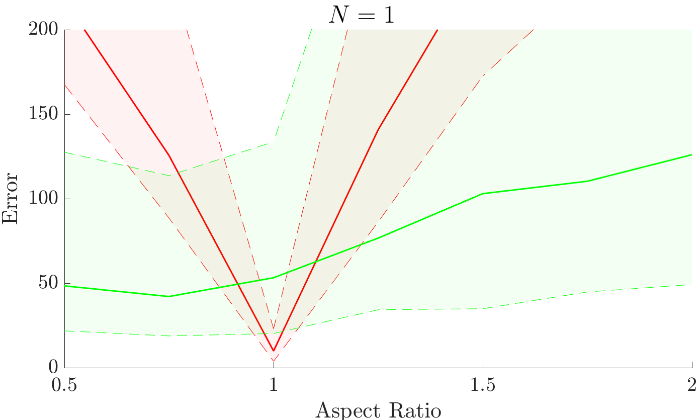
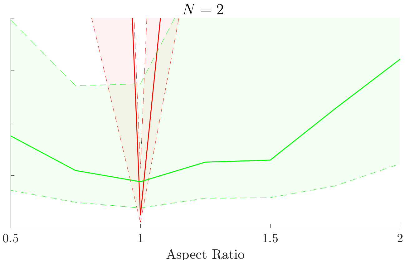
Figure C.1: Noise sensitivity. RMS reprojection error on synthetic images with added 1 px noise for (left) the solvers for the division model complexity $N=1$, and (right) the solvers for the complexity $N=2$. Red curves correspond to the linear solvers from (17) that do not solve for the aspect ratio, and green curves correspond to the aspect ratio solvers from (22). Solid curves are the median errors and the shaded plots are the corresponding interquartile ranges.

GOPRO	ENTANIYA	TUMVI
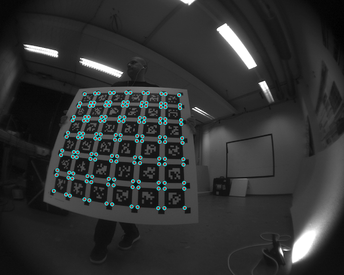
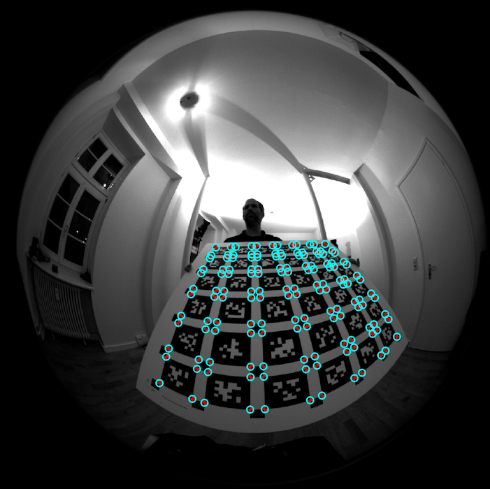
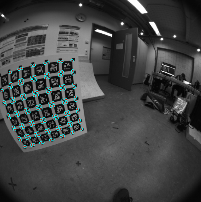
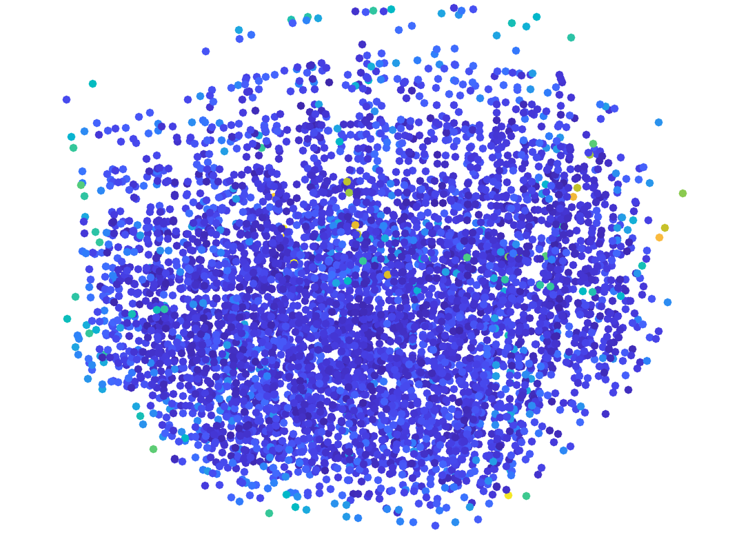
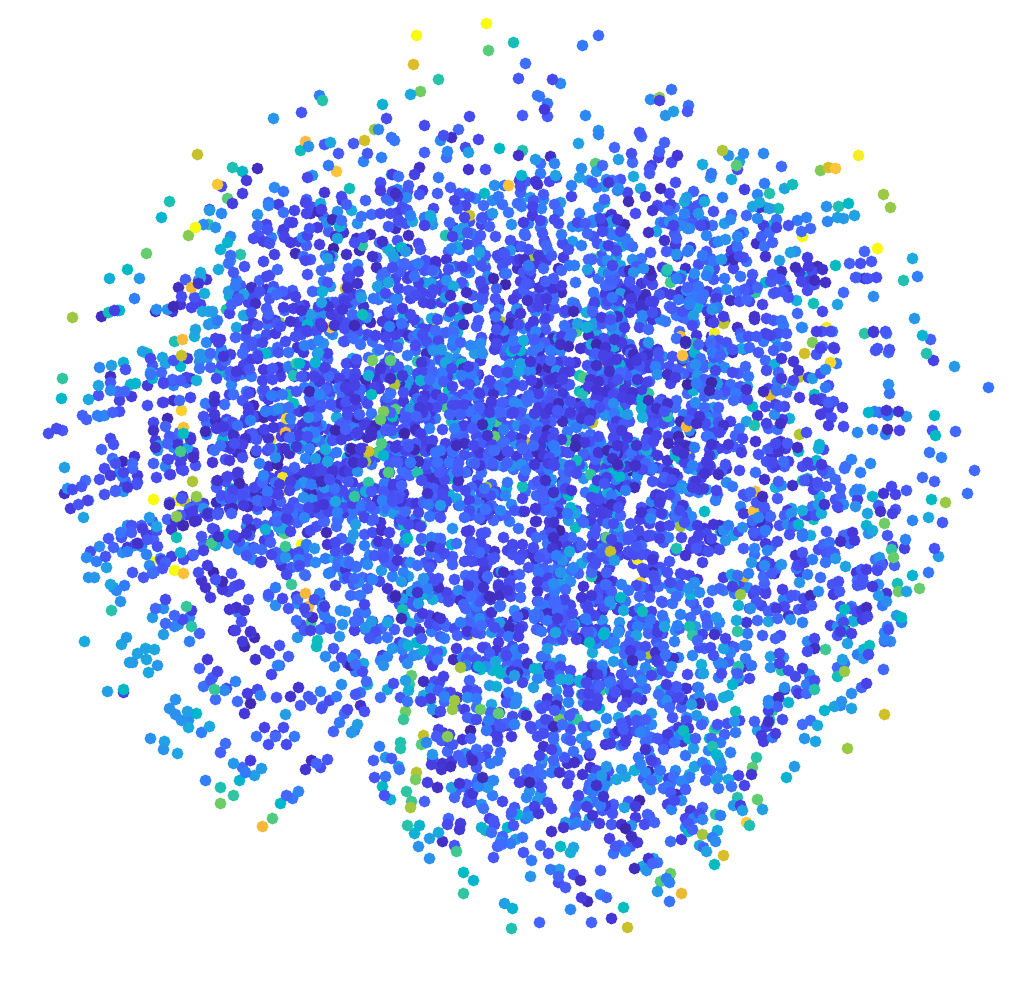
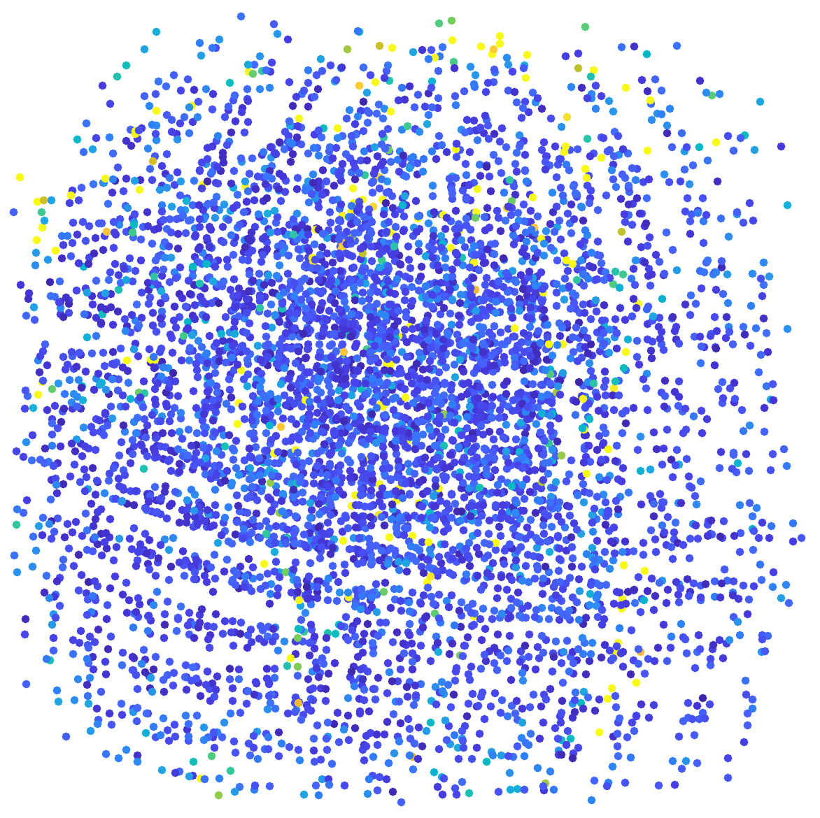
KaidanOmni	MiniOmni	VMRImage
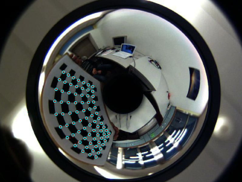
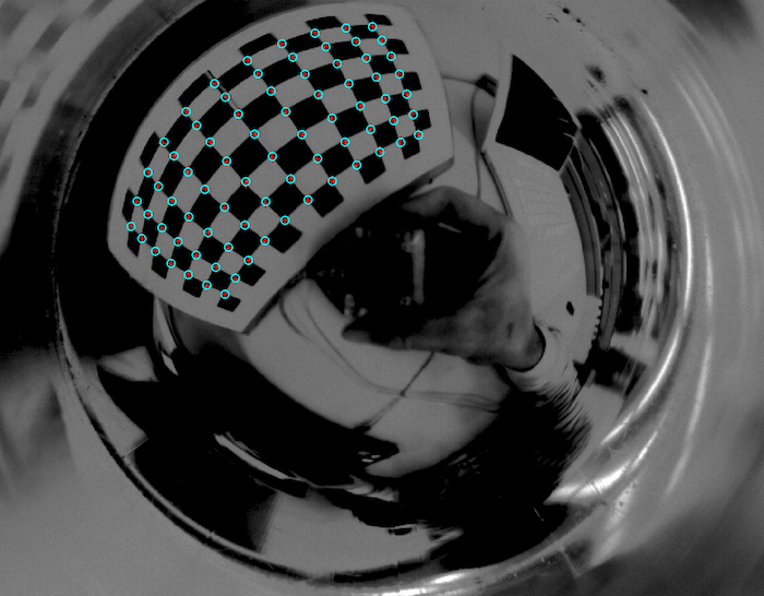
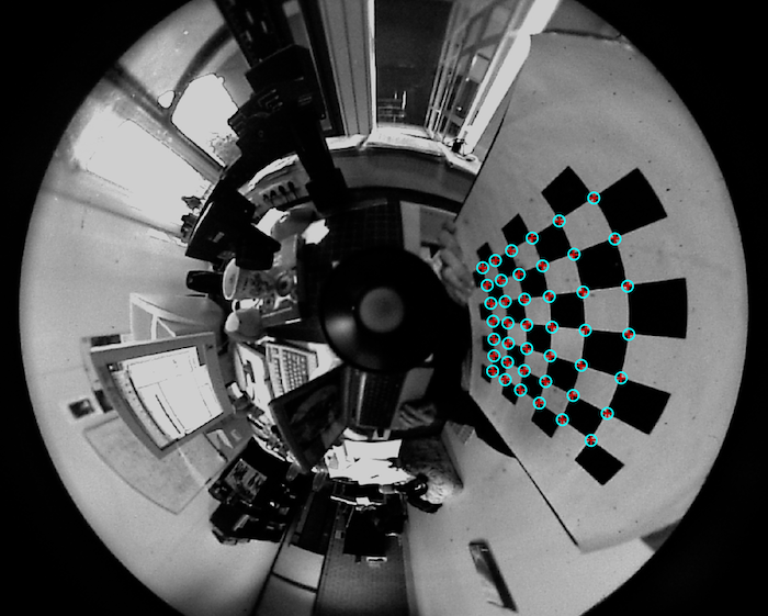
DAVIS-indoor	DAVIS-outdoor	Snapdragon

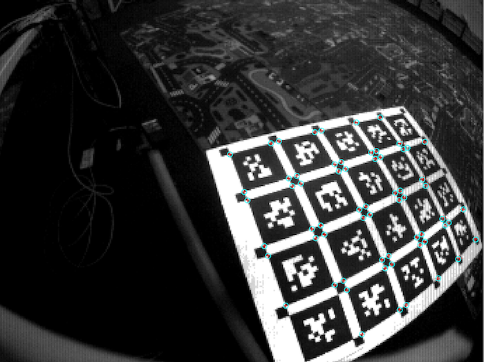
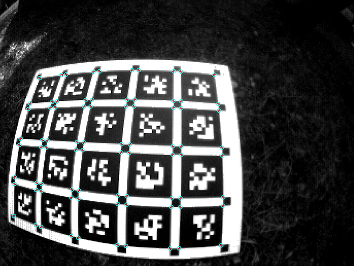
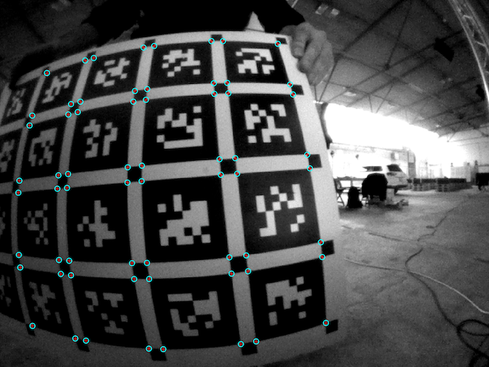
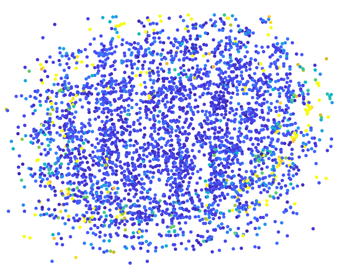
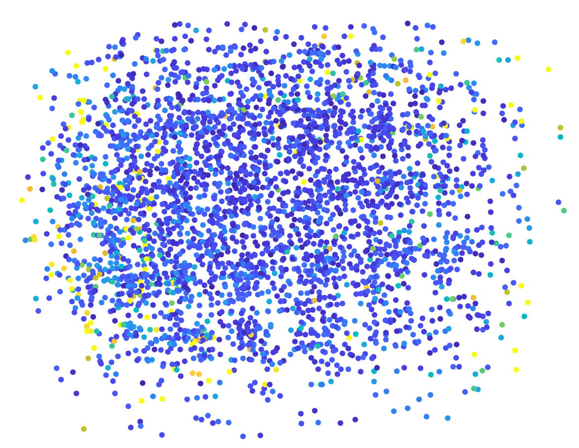
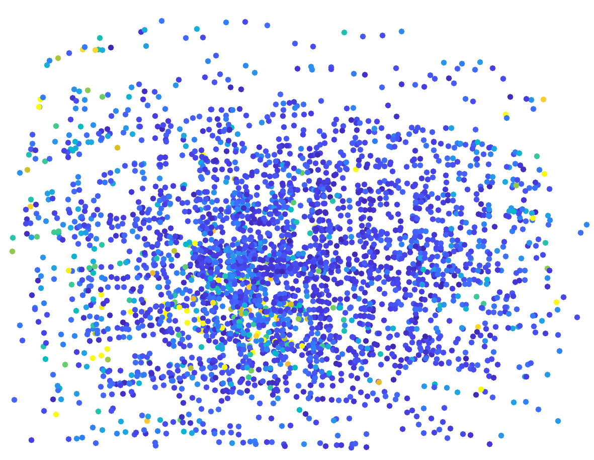
Figure C.2: Kalibr, OCamCalib and UZH data and calibration results. (rows 1,3,5) example images with detected (red crosses) and reprojected (cyan circles) corners; (rows 2,4,6) all corners from the camera subset color-coded corresponding to their reprojection errors.

Train size: 1	Train size: 2	Train size: 5

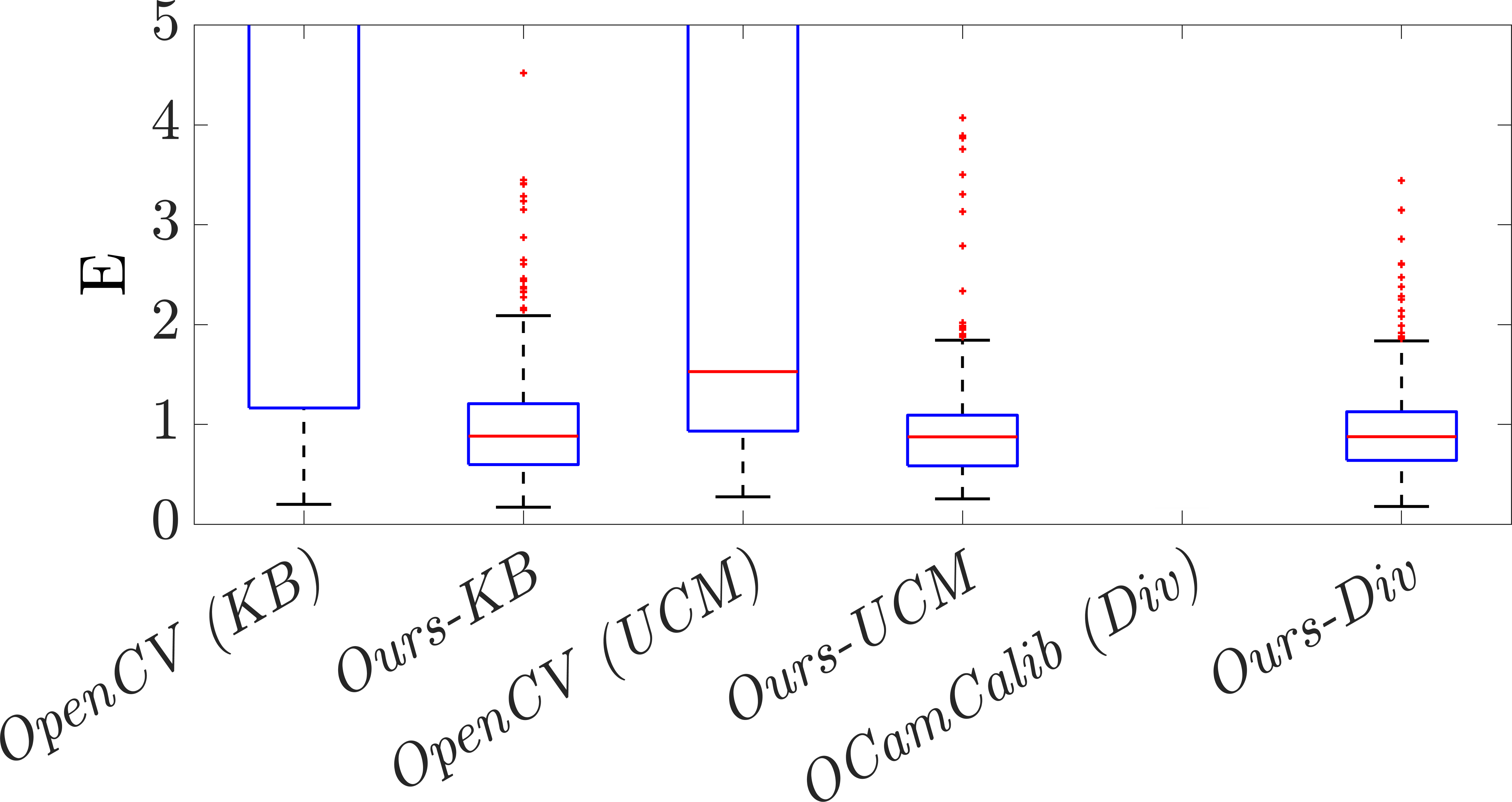
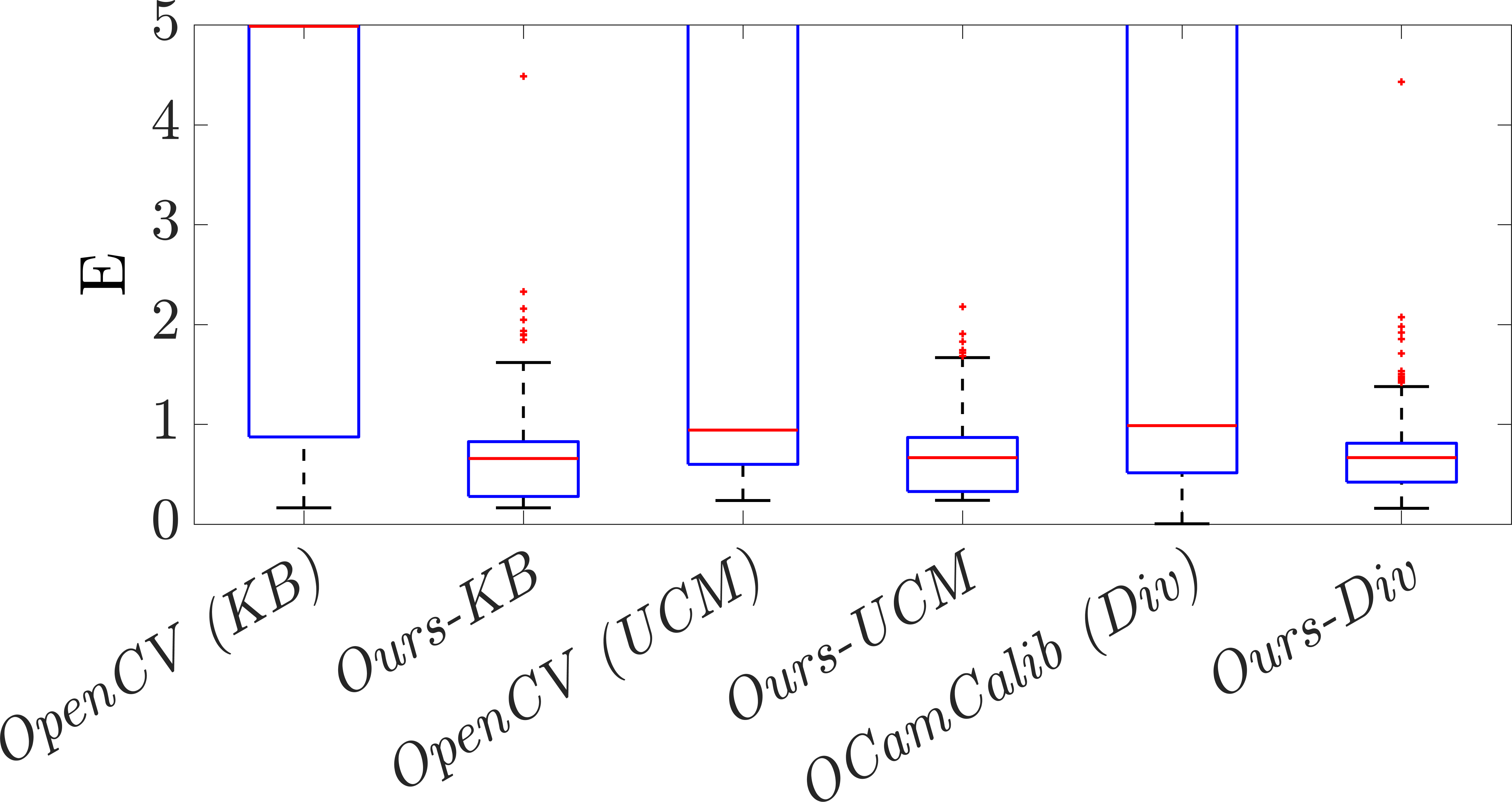
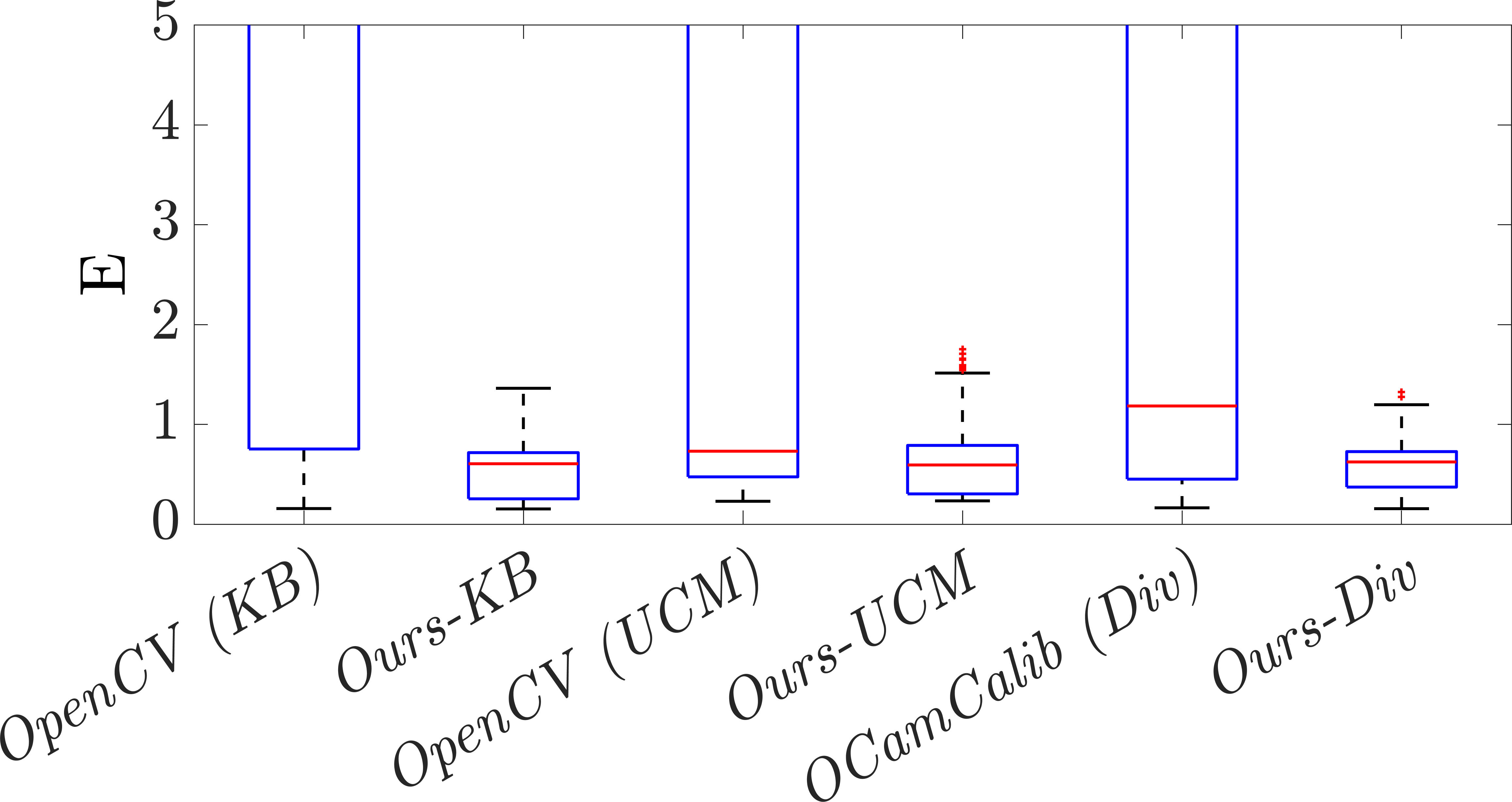
Figure C.3: Calibration results for limited train data. Cross-validation with corresponding train size is performed, and the reported errors are normalized in accordance with image resolution $1000\times 1000$ px. E denotes the RMS weighted reprojection error. OCamCalib-DIV requires at least two images for calibration.

D Calibration with Limited Data

Calibration accuracy is dependent on good feature coverage. However, fast calibration from few images is also important for users e.g. for lens inventory purposes. We compared the performance of calibration methods on a limited amount of training data starting from a single image. We randomly drew the subsamples of sizes 1, 2, and 5 images from the training data (10 times for each train size) and evaluated the calibrations on the hold-out test data. The Fig. C.3 reports the distributions of the robust test errors (19). To remove the effect of the image resolution for different cameras, the errors are normalized in accordance with the resolution $1000\times 1000$ px. There are several limitations found in current frameworks. OCamCalib-DIV requires at least two images for calibration so they don’t have the results for the train size 1. Also, as was mentioned in previous section, this toolbox requires all points to be visible from all views which is a big limitation. All other methods would occasionally fail for particular subsets of images. For such failure cases we set the test error to be the maximum error. The proposed calibration method never fails and provides the best calibration starting from a single image already.

References

- [1] Joao Pedro Barreto and Helder Araujo. Issues on the geometry of central catadioptric image formation. In Proceedings of the 2001 IEEE Computer Society Conference on Computer Vision and Pattern Recognition. CVPR 2001, volume 2, pages II–II. IEEE, 2001.
- [2] Michael Burri, Janosch Nikolic, Pascal Gohl, Thomas Schneider, Joern Rehder, Sammy Omari, Markus W Achtelik, and Roland Siegwart. The euroc micro aerial vehicle datasets. The International Journal of Robotics Research, 35(10):1157–1163, 2016.
- [3] Federico Camposeco, Torsten Sattler, and Marc Pollefeys. Non-parametric structure-based calibration of radially symmetric cameras. In Proceedings of the IEEE International Conference on Computer Vision, pages 2192–2200, 2015.
- [4] Ondřej Chum, Jiří Matas, and Josef Kittler. Locally optimized ransac. In Bernd Michaelis and Gerald Krell, editors, Pattern Recognition, pages 236–243, Berlin, Heidelberg, 2003. Springer Berlin Heidelberg.
- [5] David Claus and Andrew W Fitzgibbon. A rational function lens distortion model for general cameras. In 2005 IEEE Computer Society Conference on Computer Vision and Pattern Recognition (CVPR’05), volume 1, pages 213–219. IEEE, 2005.
- [6] Jeffrey Delmerico, Titus Cieslewski, Henri Rebecq, Matthias Faessler, and Davide Scaramuzza. Are we ready for autonomous drone racing? the UZH-FPV drone racing dataset. In IEEE Int. Conf. Robot. Autom. (ICRA), 2019.
- [7] Frederic Devernay and Olivier Faugeras. Straight lines have to be straight. Machine vision and applications, 13(1):14–24, 2001.
- [8] C Brown Duane. Close-range camera calibration. Photogramm. Eng, 37(8):855–866, 1971.
- [9] Olivier D Faugeras, Q-T Luong, and Stephen J Maybank. Camera self-calibration: Theory and experiments. In European conference on computer vision, pages 321–334. Springer, 1992.
- [10] Martin A Fischler and Robert C Bolles. Random sample consensus: a paradigm for model fitting with applications to image analysis and automated cartography. Communications of the ACM, 24(6):381–395, 1981.
- [11] Andrew W Fitzgibbon. Simultaneous linear estimation of multiple view geometry and lens distortion. In Proceedings of the 2001 IEEE Computer Society Conference on Computer Vision and Pattern Recognition. CVPR 2001, volume 1, pages I–I. IEEE, 2001.
- [12] Clive S Fraser. Digital camera self-calibration. ISPRS Journal of Photogrammetry and Remote sensing, 52(4):149–159, 1997.
- [13] Christopher Geyer and Kostas Daniilidis. A unifying theory for central panoramic systems and practical implications. In European conference on computer vision, pages 445–461. Springer, 2000.
- [14] H. Ha, M. Perdoch, H. Alismail, I. S. Kweon, and Y. Sheikh. Deltille grids for geometric camera calibration. In 2017 IEEE International Conference on Computer Vision (ICCV), pages 5354–5362, 2017.
- [15] Richard Hartley and Sing Bing Kang. Parameter-free radial distortion correction with center of distortion estimation. IEEE Transactions on Pattern Analysis and Machine Intelligence, 29(8):1309–1321, 2007.
- [16] Richard Hartley and Andrew Zisserman. Multiple view geometry in computer vision. Cambridge university press, 2003.
- [17] Richard I Hartley. Self-calibration from multiple views with a rotating camera. In European Conference on Computer Vision, pages 471–478. Springer, 1994.
- [18] Janne Heikkila and Olli Silvén. A four-step camera calibration procedure with implicit image correction. In Proceedings of IEEE computer society conference on computer vision and pattern recognition, pages 1106–1112. IEEE, 1997.
- [19] Peter J Huber. Robust statistics, volume 523. John Wiley & Sons, 2004.
- [20] Juho Kannala and Sami S Brandt. A generic camera model and calibration method for conventional, wide-angle, and fish-eye lenses. IEEE transactions on pattern analysis and machine intelligence, 28(8):1335–1340, 2006.
- [21] Bogdan Khomutenko, Gaëtan Garcia, and Philippe Martinet. An enhanced unified camera model. IEEE Robotics and Automation Letters, 1(1):137–144, 2015.
- [22] V. Larsson, T. Sattler, Z. Kukelova, and M. Pollefeys. Revisiting radial distortion absolute pose. In 2019 IEEE/CVF International Conference on Computer Vision (ICCV), pages 1062–1071, 2019.
- [23] Bo Li, Lionel Heng, Kevin Koser, and Marc Pollefeys. A multiple-camera system calibration toolbox using a feature descriptor-based calibration pattern. In 2013 IEEE/RSJ International Conference on Intelligent Robots and Systems, pages 1301–1307. IEEE, 2013.
- [24] Yaroslava Lochman, Oles Dobosevych, Rostyslav Hryniv, and James Pritts. Minimal solvers for single-view lens-distorted camera auto-calibration. In Proceedings of the IEEE/CVF Winter Conference on Applications of Computer Vision, pages 2887–2896, 2021.
- [25] Jérôme Maye, Paul Furgale, and Roland Siegwart. Self-supervised calibration for robotic systems. In 2013 IEEE Intelligent Vehicles Symposium (IV), pages 473–480. IEEE, 2013.
- [26] Christopher Mei and Patrick Rives. Single view point omnidirectional camera calibration from planar grids. In Proceedings 2007 IEEE International Conference on Robotics and Automation, pages 3945–3950. IEEE, 2007.
- [27] Branislav Micusik and Tomas Pajdla. Estimation of omnidirectional camera model from epipolar geometry. In 2003 IEEE Computer Society Conference on Computer Vision and Pattern Recognition, 2003. Proceedings., volume 1, pages I–I. IEEE, 2003.
- [28] Gaku Nakano. A simple direct solution to the perspective-three-point problem. In Kirill Sidorov and Yulia Hicks, editors, Proceedings of the British Machine Vision Conference (BMVC), pages 102.1–102.12. BMVA Press, September 2019.
- [29] Edwin Olson. Apriltag: A robust and flexible visual fiducial system. In 2011 IEEE International Conference on Robotics and Automation, pages 3400–3407. IEEE, 2011.
- [30] Marc Pollefeys, Reinhard Koch, and Luc Van Gool. Self-calibration and metric reconstruction inspite of varying and unknown intrinsic camera parameters. International Journal of Computer Vision, 32(1):7–25, 1999.
- [31] James Pritts, Zuzana Kukelova, Viktor Larsson, Yaroslava Lochman, and Ondřej Chum. Minimal solvers for rectifying from radially-distorted conjugate translations. IEEE Transactions on Pattern Analysis and Machine Intelligence, 2020.
- [32] Srikumar Ramalingam and Peter Sturm. A unifying model for camera calibration. IEEE transactions on pattern analysis and machine intelligence, 39(7):1309–1319, 2016.
- [33] Srikumar Ramalingam, Peter Sturm, and Suresh K Lodha. Towards complete generic camera calibration. In 2005 IEEE Computer Society Conference on Computer Vision and Pattern Recognition (CVPR’05), volume 1, pages 1093–1098. IEEE, 2005.
- [34] Davide Scaramuzza, Agostino Martinelli, and Roland Siegwart. A flexible technique for accurate omnidirectional camera calibration and structure from motion. In Fourth IEEE International Conference on Computer Vision Systems (ICVS’06), pages 45–45. IEEE, 2006.
- [35] Davide Scaramuzza, Agostino Martinelli, and Roland Siegwart. A toolbox for easily calibrating omnidirectional cameras. In 2006 IEEE/RSJ International Conference on Intelligent Robots and Systems, pages 5695–5701. IEEE, 2006.
- [36] Thomas Schops, Viktor Larsson, Marc Pollefeys, and Torsten Sattler. Why having 10,000 parameters in your camera model is better than twelve. In Proceedings of the IEEE/CVF Conference on Computer Vision and Pattern Recognition, pages 2535–2544, 2020.
- [37] David Schubert, Thore Goll, Nikolaus Demmel, Vladyslav Usenko, Jörg Stückler, and Daniel Cremers. The TUM VI benchmark for evaluating visual-inertial odometry. In 2018 IEEE/RSJ International Conference on Intelligent Robots and Systems (IROS), pages 1680–1687. IEEE, 2018.
- [38] Peter Sturm and Srikumar Ramalingam. A generic concept for camera calibration. In European Conference on Computer Vision, pages 1–13. Springer, 2004.
- [39] Peter Sturm and Srikumar Ramalingam. Camera models and fundamental concepts used in geometric computer vision. Now Publishers Inc, 2011.
- [40] Steffen Urban, Jens Leitloff, and Stefan Hinz. Improved wide-angle, fisheye and omnidirectional camera calibration. ISPRS Journal of Photogrammetry and Remote Sensing, 108:72–79, 2015.
- [41] Vladyslav Usenko, Nikolaus Demmel, and Daniel Cremers. The double sphere camera model. In 2018 International Conference on 3D Vision, 3DV 2018, Verona, Italy, September 5-8, 2018, pages 552–560. IEEE Computer Society, 2018.
- [42] Horst Wildenauer and Allan Hanbury. Robust camera self-calibration from monocular images of manhattan worlds. In 2012 IEEE Conference on Computer Vision and Pattern Recognition, pages 2831–2838, 2012.
- [43] Z. Zhang. A flexible new technique for camera calibration. IEEE Transactions on Pattern Analysis and Machine Intelligence, 22(11):1330–1334, 2000.
- [44] Zichao Zhang, Henri Rebecq, Christian Forster, and Davide Scaramuzza. Benefit of large field-of-view cameras for visual odometry. In 2016 IEEE International Conference on Robotics and Automation (ICRA), pages 801–808. IEEE, 2016.