Learning to Forecast Dynamical Systems from Streaming Data

Abstract

Kernel analog forecasting (KAF) is a powerful methodology for data-driven, non-parametric forecasting of dynamically generated time series data. This approach has a rigorous foundation in Koopman operator theory and it produces good forecasts in practice, but it suffers from the heavy computational costs common to kernel methods. This paper proposes a streaming algorithm for KAF that only requires a single pass over the training data. This algorithm dramatically reduces the costs of training and prediction without sacrificing forecasting skill. Computational experiments demonstrate that the streaming KAF method can successfully forecast several classes of dynamical systems (periodic, quasi-periodic, and chaotic) in both data-scarce and data-rich regimes. The overall methodology may have wider interest as a new template for streaming kernel regression.

37Nxx, 65Pxx, 65Fxx, 62Jxx

1 Introduction

Forecasting problems are ubiquitous in physical science and engineering applications, including climate prediction [64], navigation [68], and medicine [43]. In these settings, we do not possess complete information about the state of the system, and we may not have full knowledge of the equations of motion. Owing to our lack of omniscience, it is not possible to make predictions by integrating the current state forward in time. Instead, we may acquire training data by observing some aspect of the system’s evolution. The goal is to build a compact model of the dynamics of this observable. Given a new observation, the model should allow us to forecast the future trajectory from the initial condition.

Kernel analog forecasting (KAF) [1] offers a promising approach to this problem. KAF is a data-driven, non-parametric forecasting technique that is best understood as a type of regularized kernel regression (Section 2). KAF emerged from recent efforts [9] to translate Koopman operator theory into effective computational methodologies for forecasting (Section 2.7). The approach belongs to a rapidly expanding literature [59, 24, 12, 53, 47] on operator-theoretic techniques for low-order modeling of dynamical systems, including methods [8, 84, 45, 38] based on kernels.

KAF is mathematically rigorous, and it provides good-quality predictions for benchmark examples [1]. Nevertheless, the straightforward implementation (“naïve KAF”) has several weaknesses. First, naïve KAF requires multiple views of the training data, so it cannot operate in the “streaming” setting where we only see the training data once (Section 3.1). Second, the process of constructing the model is computationally expensive: to form the kernel matrix, the costs of arithmetic and storage are both quadratic in the length of the training data. Third, the basic method must store all of the training data to make predictions, so the forecasting model is quite large. Fourth, the arithmetic cost of a single forecast is linear in the amount of training data. These issues have limited the applicability of the KAF methodology.

In response to this challenge, we propose a novel streaming KAF algorithm (Section 3). Our approach depends on two prominent techniques from the field of randomized matrix computation [57]: random Fourier features [69] for kernel approximation and the randomized Nyström method [36, 31, 52, 78, 57] for streaming PCA. Overall, the streaming KAF method builds a model using time and storage linear in the amount of training data, and it can make forecasts with time and storage that are independent of the amount of training data.

Computational experiments (Section 4) demonstrate that streaming KAF is a practical method for making predictions of two benchmark dynamical systems: Lorenz ’63 (L63) [55] and two-level Lorenz ’96 (L96) [22]. In particular, streaming KAF exhibits forecasting skill similar to naïve KAF in a range of situations, including systems that are periodic, quasi-periodic, and chaotic. At the same time, streaming KAF can operate in settings where naïve KAF is prohibitively expensive, including cases where the observables are high-dimensional or the amount of training data is enormous. In the data-rich setting, after just a few minutes of training time, streaming KAF can drive the forecasting error toward zero. As a consequence, we believe that the streaming KAF algorithm has the potential to unlock the full potential of KAF as a forecasting methodology.

Remark 1.1 (Prior work).

Although developed independently, our methodology is related to recent papers that apply random features to perform streaming kernel principal component analysis [27, 81] and kernel ridge regression [5, 71]. The details of our algorithm are somewhat different from these works, and we believe that our work yields a novel approach for streaming kernel regression. We have also studied a streaming KAF algorithm based on AdaOja [41], an adaptive variant of Oja’s algorithm, which is a competitive alternative to the Nyström method [40]. See Section 5 for more discussion of related work.

1.1 Outline

Section 2 motivates the existing KAF procedure as a form of regularized kernel regression that is specifically designed for dynamical systems. Section 3 describes how to develop a streaming implementation of KAF. In particular, we discuss kernel approximation via random Fourier features and the randomized Nyström method. Finally, Section 4 presents computational experiments which demonstrate that our methodology is effective for two classical dynamical systems.

1.2 Notation

Throughout, we work in a real Euclidean space $\mathbbm{R}^{d}$ equipped with the $\ell_{2}$ norm $\left\|\cdot\right\|$ and inner product $\langle\cdot,\cdot\rangle$. The methodology and results should extend to the complex field $\mathbb{C}$. Matrices (such as $\bm{M}\in\mathbbm{R}^{d\times n}$) are written as bold capitals, vectors ($\bm{v}\in\mathbbm{R}^{d}$) are written as bold lowercase, and scalars ($x\in\mathbbm{R}$) are written in plain lowercase.

Every matrix $\bm{M}\in\mathbbm{R}^{d\times n}$ admits a compact singular value decomposition (SVD), a matrix factorization $\bm{M}=\bm{U}\bm{\Sigma}\bm{V}^{\top}$ with the following properties. For $r\coloneqq\operatorname{rank}(\bm{M})\leq\min\{d,n\}$, the left and right singular vector matrices $\bm{U}\in\mathbbm{R}^{d\times r}$ and $\bm{V}\in\mathbbm{R}^{r\times n}$ have orthonormal columns. The matrix $\bm{\Sigma}=\operatorname{diag}(\sigma_{1},\sigma_{2},\dots,\sigma_{r})\in\mathbbm{R}^{r\times r}$ is positive and diagonal, with its diagonal elements (the singular values) arranged in decreasing order: $\sigma_{1}\geq\sigma_{2}\geq\dots\geq\sigma_{r}>\sigma_{r+1}\coloneqq 0$. Singular values are uniquely determined, but singular vectors are not.

Given an SVD of the rank-$r$ matrix $\bm{M}$, we can define the Moore–Penrose pseudoinverse $\bm{M}^{\dagger}\coloneqq\bm{V}\bm{\Sigma}^{-1}\bm{U}^{\top}$ where $\bm{\Sigma}^{-1}\coloneqq\operatorname{diag}(\sigma_{1}^{-1},\dots,\sigma_{r}^{-1})\in\mathbbm{R}^{r\times r}$. The pseudoinverse coincides with the matrix inverse for a full-rank, square matrix.

The operator norm $\left\|\bm{M}\right\|\coloneqq\sigma_{1}$ equals the largest singular value $\sigma_{1}$. The Frobenius norm $\left\|\bm{M}\right\|_{\mathrm{F}}\coloneqq(\sum_{i=1}^{r}\sigma_{i}^{2})^{1/2}$ is the $\ell_{2}$ norm of the singular values.

For any rank parameter $\ell\leq r$, we can construct an $\ell$-truncated SVD $\llbracket\bm{M}\rrbracket_{\ell}\coloneqq\bm{U}\bm{\Sigma}_{\ell}\bm{V}^{\top}$ where $\bm{\Sigma}_{\ell}\coloneqq\operatorname{diag}(\sigma_{1},\sigma_{2},\dots,\sigma_{\ell},0,\dots,0)\in\mathbbm{R}^{r\times r}$ retains only the leading $\ell$ singular values. The matrix $\llbracket\bm{M}\rrbracket_{\ell}$ is a best rank-$r$ approximation of $\bm{M}$ with respect to both the operator norm and the Frobenius norm. In the case $\sigma_{\ell}=\sigma_{\ell+1}$, the truncated SVD $\llbracket\bm{M}\rrbracket_{\ell}$ depends on the underlying choice of SVD, so this notation should be interpreted with care.

2 Introduction to KAF

Suppose we have access to snapshots of a discrete dynamical system as it evolves in time, and we would like to forecast its future values. Let us begin with the most basic setting; we will discuss more general observation models in Section 2.6.

To formalize the problem, let ${\cal M}\subseteq\mathbbm{R}^{d}$ be a closed subset of a Euclidean space. We call ${\cal M}$ the state space. Let $F:{\cal M}\rightarrow{\cal M}$ be a mapping, called the flow map. Suppose that we observe an initial condition $\bm{x}_{0}\in{\cal M}$ as well as the (partial) trajectory $\bm{x}_{1},\bm{x}_{2},\dots,\bm{x}_{n-1}\in{\cal M}$ obtained by iterating the flow map:

(1) $$\bm{x}_{j}=F(\bm{x}_{j-1})=F^{j}(\bm{x}_{0})\quad\text{for $j=1,2,\dots,n-1$.}$$

In most settings, we do not actually know the flow map $F$. Rather, the goal is to use information latent in the measured trajectory $(\bm{x}_{0},\dots,\bm{x}_{n-1})$ to infer the dynamics. Afterward, we are given a new initial condition $\bm{y}\in\mathcal{M}$, and we are asked to forecast the future state $F^{q}(\bm{y})$ of the system after $q$ time steps.

2.1 Linear forecasting

To motivate the KAF method, we first describe an earlier approach to the forecasting problem, based on linear inverse models (LIMs) [66] and the closely related dynamic mode decomposition (DMD) [70, 73, 79, 47]. Fix a forecasting horizon $q\in\mathbb{N}$. We can arrange the observed trajectory $\bm{x}_{0},\bm{x}_{1},\dots,\bm{x}_{n-1},\bm{x}_{n},\dots,\bm{x}_{n+q-1}\in\mathbbm{R}^{d}$ into a training data set that consists of input–response pairs: $\{(\bm{x}_{j},\bm{x}_{j+q})\}_{j=0}^{n-1}$. Equivalently, consider the pair of matrices

(2) $$\bm{X} \coloneqq\begin{bmatrix}\bm{x}_{0}&\bm{x}_{1}&\dots&\bm{x}_{n-1}\end{bmatrix}\in\mathbbm{R}^{d\times n};$$

(3) $$\quad\bm{X}_{[+q]} \coloneqq\begin{bmatrix}\bm{x}_{q}&\bm{x}_{q+1}&\dots&\bm{x}_{n+q-1}\end{bmatrix}\in\mathbbm{R}^{d\times n}.$$

We can attempt to find the best linear model $\bm{A}:\mathbbm{R}^{d}\to\mathbbm{R}^{d}$ for the dynamics by means of a least-squares fit:

(4) $$\bm{A}\in\underset{\bm{M}\in\mathbbm{R}^{d\times d}}{\arg\min}\ \sum_{j=0}^{n-1}\left\|\bm{M}\bm{x}_{j}-\bm{x}_{j+q}\right\|^{2}=\underset{\bm{M}\in\mathbbm{R}^{d\times d}}{\arg\min}\ \left\|\bm{M}\bm{X}-\bm{X}_{[+q]}\right\|_{\mathrm{F}}^{2}.$$

An optimal solution to this problem is the matrix

(5) $$\bm{A}=\bm{X}_{[+q]}\bm{X}^{\dagger}\in\mathbbm{R}^{d\times d}.$$

Suppose we are given a state $\bm{y}\in\mathbbm{R}^{d}$ that serves as a new initial condition. We can forecast the state $\bm{y}_{[+q]}\coloneqq F^{q}(\bm{y})$ after $q$ time steps via the estimate $\bm{y}_{[+q]}\approx\bm{A}\bm{y}$. In other words, $\bm{A}$ serves as a linear approximation to the iterated flow map $F^{q}$.

Let us manipulate the linear model for the dynamics so that it takes a more suggestive form. Recall that the pseudoinverse satisfies $\bm{X}^{\dagger}=(\bm{X}^{\top}\bm{X})^{\dagger}\bm{X}^{\top}$. Therefore,

$$\bm{A}=\bm{X}_{[+q]}(\bm{X}^{\top}\bm{X})^{\dagger}\bm{X}^{\top}.$$

Given a new initial condition $\bm{y}\in\mathbbm{R}^{d}$, we obtain the linear forecast

(6) $$\tilde{\bm{y}}_{[+q]}\coloneqq\bm{A}\bm{y}=\bm{X}_{[+q]}(\bm{X}^{\top}\bm{X})^{\dagger}(\bm{X}^{\top}\bm{y})\in\mathbbm{R}^{d}.$$

Observe that this computation can be formulated in terms of inner products between states.

2.2 The kernel trick

Of course, dynamical systems of practical interest are highly nonlinear, so linear approximations are only valid over a short time horizon. When one needs to process data with nonlinear structure, a general principle is to “lift and linearize”. That is, we apply a nonlinear map to transport the data to a high-dimensional space where it may have linear structure; we implement a linear fitting algorithm on the high-dimensional space; and then we project back down to the original domain to obtain a (nonlinear) low-dimensional model for the data. This approach gives rise to KAF, discussed below, as well as other data-driven analysis and forecasting techniques [84, 45, 48, 38].

Remarkably, this lifting technique can often be implemented without applying the nonlinear map explicitly. Consider a method, such as Eq. 6, that processes Euclidean data using the inner product as a measure of the similarity between data points. The kernel trick allows us to develop a nonlinear extension simply by replacing each inner product $\bm{x}^{\top}\bm{y}$ in the data space with a more general function $\kappa(\bm{x},\bm{y})$, called a kernel.

The kernel trick is justified by the Moore–Aronszajn theorem [4, section 2(4)]. Let $\kappa:\mathbbm{R}^{d}\times\mathbbm{R}^{d}\to\mathbbm{R}$ be a symmetric, positive-definite function. That is,

$$\begin{bmatrix}\kappa(\bm{v}_{i},\bm{v}_{j})\end{bmatrix}_{i,j=1}^{n}\quad\text{is positive definite for every $n\in\mathbb{N}$ and $\bm{v}_{1},\dots,\bm{v}_{n}\in\mathbbm{R}^{d}$.}$$

Then, the kernel function $\kappa$ coincides with the inner product on a Hilbert space $\cal{H}$. More precisely, there is a nonlinear feature map $\varphi:\mathbbm{R}^{d}\to\cal{H}$ with the property that $\kappa(\bm{x},\bm{y})=\langle\varphi(\bm{x}),\varphi(\bm{y})\rangle_{\mathcal{H}}$ for all $\bm{x},\bm{y}\in\mathbbm{R}^{d}$. Implicitly, the feature map summarizes each data point $\bm{x}$ by a long list $\varphi(\bm{x})\in{\cal H}$ of features, and the kernel computes the inner product between the feature vectors.

One of the most popular kernel functions is the Gaussian radial basis function (RBF) kernel. For an inverse bandwidth parameter $\gamma>0$, this kernel takes the form

(7) $$\kappa(\bm{x},\bm{y})\coloneqq\mathrm{e}^{-\gamma\left\|\bm{x}-\bm{y}\right\|^{2}}\quad\text{for $\bm{x},\bm{y}\in\mathbbm{R}^{d}$.}$$

Under this kernel, two points are “similar” precisely when they are close enough together in Euclidean distance, where the scale depends on the choice of $\gamma$. For clarity of presentation, we will work exclusively with the Gaussian RBF kernel in this paper.

2.3 Nonlinear kernel forecasting

We can apply the kernel trick to the linear forecasting model Eq. 6. Indeed, we may replace the inner-products in the forms $\bm{X}^{\top}\bm{X}$ and $\bm{X}^{\top}\bm{y}$ by their kernel equivalents:

$$\bm{K}_{x,x}\coloneqq\big{[}\kappa(\bm{x}_{i},\bm{x}_{j})\big{]}_{i,j}\in\mathbbm{R}^{n\times n}\quad\text{and}\quad\bm{K}_{x,y}\coloneqq\big{[}\kappa(\bm{x}_{i},\bm{y})\big{]}_{i}\in\mathbbm{R}^{n}.$$

This step leads to the kernel analog forecast

(8) $$f_{q}(\bm{y})\coloneqq\bm{X}_{[+q]}(\bm{K}_{x,x})^{\dagger}\bm{K}_{x,y}\in\mathbbm{R}^{d}.$$

The forecast Eq. 8 provides a natural nonlinear generalization of the linear forecast Eq. 6.

2.4 Regularization

It is dangerous to implement the formula Eq. 8 as written because kernel matrices, such as $\bm{K}_{x,x}$, are notoriously ill-conditioned; for example, see [7]. As a consequence, the method Eq. 8 can be sensitive to small changes in the observed data.

The paper [1] proposes a mechanism for stabilizing the nonlinear forecast Eq. 8 by replacing the kernel matrix $\bm{K}_{x,x}$ with its best rank-$\ell$ approximation $\llbracket\bm{K}_{x,x}\rrbracket_{\ell}$, where $\ell\in\mathbb{N}$ is a parameter. In practice, we must also shift the kernel matrix by $\mu\mathbf{I}$ by a small parameter $\mu$ to avoid numerical problems. These modifications leads to the stabilized kernel analog forecast

(9) $$f_{q,\ell}(\bm{Y})\coloneqq\bm{X}_{[+q]}(\llbracket\bm{K}_{x,x}+\mu\mathbf{I}\rrbracket_{\ell})^{\dagger}\bm{K}_{x,y}.$$

The dimension $\ell$ of the regression model is usually modest (say, 100s or 1000s); it increases slowly with the required accuracy of the forecasts. The shift parameter $\mu$ is taken to be a small fixed value, such as $10^{-6}\left\|\bm{K}_{x,x}\right\|$.

The forecasting method Eq. 9 is rigorously justified in [1]. We can view the approach as a form of regularized least-squares [39, 82, 10] on the feature space induced by the kernel. It is closely related to kernel ridge regression [74].

2.5 Resource usage

The KAF method Eq. 9 involves two phases. In the training step, we use the trajectory data $\bm{X}$ to compute a matrix of prediction weights. In the forecasting step, we use the trajectory data and the test state $\bm{y}$ to make the forecast. Let us summarize the resource usage of an uninspired implementation of the KAF procedure (“naïve KAF”). See Table 1 for a summary of this discussion.

In the training phase, we first construct the $n\times n$ kernel matrix $\bm{K}_{x,x}$. This step involves $O(dn^{2})$ arithmetic and $O(n^{2})$ storage. The quadratic dependency on the number $n$ of training samples is a severe bottleneck that prevents us from performing KAF at scale.

Next, we must compute the $\ell$-truncated eigenvalue decomposition of the kernel matrix $\bm{K}_{x,x}$. Classical algorithms can succeed with $O(\ell^{2}n)$ arithmetic operations and $O(\ell n)$ storage. Nevertheless, dense methods require random access to the kernel matrix, while Krylov methods require a long sequence of matrix–vector multiplies with the kernel matrix [32]. Moreover, these algorithms are not fully reliable [52].

Third, we form the matrix $\bm{W}\coloneqq\bm{X}_{[+q]}(\llbracket\bm{K}_{x,x}+\mu\mathbf{I}\rrbracket_{\ell})^{\dagger}\in\mathbbm{R}^{d\times n}$ of prediction weights. Using the factorized form of the eigenvalue decomposition, this product costs $O(d\ell n)$ operations. The weight matrix requires storage $O(dn)$, which is comparable to the cost of storing the original trajectory data.

To make a forecast from a single initial condition $\bm{y}\in\mathbbm{R}^{d}$, we need to perform the kernel computation $\bm{K}_{x,y}\in\mathbbm{R}^{n}$. The cost is $O(dn)$ operations and $O(n)$ storage. To complete the forecast, we form the matrix–vector product $\bm{W}\bm{K}_{x,y}$, at a cost of $O(dn)$ operations. The linear dependency on the number $n$ of training points means that forecasting is very expensive.

2.6 Other observables

The KAF methodology extends to a wider setting. Section 3 provides full details for a streaming KAF algorithm at this level of generality. For now, we just sketch the idea.

Suppose that we observe the value of a function $u:\mathcal{M}\to\mathcal{N}$ of the state, which is called a covariate. For simplicity, we will always take $\mathcal{N}=\mathbbm{R}^{d^{\prime}}$. Given an observed covariate $u(\bm{x})$, we would like to predict a function $g:\mathcal{M}\to\mathbbm{R}^{r}$ of the state $\bm{x}$, which is called a response variable. Functions of the state, such as $g$ and $u$, are called observables.

We can build a kernel analog forecast for future values of the response by introducing a kernel $\tilde{\kappa}:\mathbbm{R}^{d^{\prime}}\times\mathbbm{R}^{d^{\prime}}$ on the covariate space. Roughly speaking, we replace the matrix $\bm{X}$ of training state data by observed covariate values $[u(\bm{x}_{0}),...,u(\bm{x}_{n-1})]\in\mathbbm{R}^{d^{\prime}\times n}$. Replace the matrix $\bm{X}_{[q]}$ of lagged state data by the lagged matrix $[g(\bm{x}_{q}),...,g(\bm{x}_{n+q-1})]\in\mathbbm{R}^{r\times n}$ of observed response variables. Repeat the derivation above to obtain a KAF function $g_{\ell,q}$ for predicting the observable $g$ from the covariate $u$.

The computational costs are similar to the costs of the basic KAF method, but the state dimension $d$ is replaced by either the covariate dimension $d^{\prime}$ or the response variable dimension $r$, depending on the role of the state in the computation. See Table 2 for an accounting.

2.7 Connection with Koopman operator theory

The linear approach Eq. 6 to forecasting was originally proposed in the paper [66], and the nonlinear kernel forecast Eq. 8 was presented in [85]. The paper [79] clarifies the connection between the nonlinear forecast and Koopman operator theory [21]. The paper [1] shows that KAF approximates the expectation of the response variable under the action of the Koopman operator, conditioned on the covariate data observed at forecast initialization. Here is an informal summary of these ideas.

In plain language, the classical work of Koopman and von Neumann [49, 50] characterizes a dynamical system through its induced action on a linear space of observables. As a basic example, a real-valued function $g:{\cal M}\to\mathbbm{R}$ on the state space is an observable of the dynamical system. The Koopman operator ${\cal K}$ is a linear operator on the space of observables that acts by composition with the flow map of the dynamics: $({\cal K}g)(\bm{x})\coloneqq(g\circ F)(\bm{x})=g(F(\bm{x}))$. Regardless of the complexity of the dynamical system, we can understand its behavior by spectral analysis of the linear operator ${\cal K}$ on an appropriately chosen Banach space of observables [6, 21]. In particular, since our state space $\mathcal{M}$ is a subset of $\mathbb{R}^{d}$, we can represent every state $\bm{x}\in\mathcal{M}$ by the “identity” observable, $\iota:\mathcal{M}\to\mathbb{R}^{d}$ with $\iota(\bm{x})=\bm{x}$. Thus, the dynamical system becomes linear when lifted to a sufficiently high-dimensional space of observables: $F(\bm{x})=(\mathcal{K}\iota)(\bm{x})$. Using similar ideas, we can also represent dynamical systems with infinite-dimensional state spaces by means of linear Koopman operators.

Building on previous work [86, 2, 17], the recent paper [1] established that the stabilized forecast Eq. 9 is a rigorous approximation of the Koopman dynamics of observables in the limit of large data. Consider a measure-preserving and ergodic dynamical system $F$, and let $[\bm{x}_{0},\dots,\bm{x}_{n-1}]$ be a state trajectory as in Eq. 1. Suppose we acquire training data in the form of covariate–response pairs $(\bm{u}_{0},\bm{g}_{q}),\dots,(\bm{u}_{n-1},\bm{g}_{q+n-1})$, where $\bm{u}_{i}=u(\bm{x}_{i})\in\mathcal{N}$ and $\bm{g}_{i}=g(\bm{x}_{i})\in\mathbbm{R}^{r}$. We may construct the KAF function $g_{\ell,q}$ as summarized in Section 2.6. Let $\bm{y}\in\mathcal{M}$ be an initial condition with an observed covariate $u(\bm{y})$. Then the kernel analog forecast converges to the conditional expectation of the response under the Koopman operator, given the covariate data at forecast initialization:

$$g_{q,\ell}(\bm{v})\to\mathbb{E}[(\mathcal{K}^{q}g)(\bm{y})\,|\,u(\bm{y})=\bm{v}]\quad\text{in $L_{2}$ as $\ell,n\to\infty$.}$$

The conditional expectation is the optimal $L_{2}$ approximation to the Koopman evolution $(\mathcal{K}^{q}g)(\bm{y})$, given only the measured covariate $\bm{v}$. In the specific case where the observables $g=u=\iota$ reproduce the full state vector, we deduce that the forecast $f_{q,\ell}(\bm{y})$ presented in Eq. 9 converges to the true $q$-step dynamical evolution, $F^{q}(\bm{y})$.

3 Streaming KAF

While KAF is rigorously justified in the limit of large data, it also becomes prohibitively expensive to implement because of its storage and arithmetic costs (Section 2.5). Indeed, the time required to construct the kernel matrix is quadratic in the length $n$ of training data. The time required to make a single forecast is linear in $n$. Furthermore, we need multiple views of the training data to build the model and another view to make a forecast, so the algorithm cannot operate in the streaming setting.

In this section, we will develop a streaming KAF method that resolves each of these issues. Our algorithm processes the trajectory data in a single pass. It reduces the arithmetic cost of training to be linear in the number $n$ of training points, and the cost of each forecast becomes independent of the amount of training data. It also limits the storage needed for the computations and for the forecasting model. Experiments (Section 4) show that the streaming KAF method is competitive with the original KAF method in forecasting skill on problem sizes where the original KAF method is tractable. But streaming KAF can achieve significantly better forecasts than naïve KAF because the streaming method can ingest large amounts of training data and resolve the dynamics more accurately.

3.1 Streaming data

Streaming data models have become popular for working with time series that have many elements, especially in high dimensions or in cases where the data arrives at high velocity [60]. The key features of a streaming data model are that (1) the elements of the time series are presented in sequential order; (2) we must process each datum at the time it arrives; and (3) we do not have sufficient storage to maintain the entire time series. The goal is to extract enough information to answer a particular set of questions about the observed data. These constraints necessitate algorithms that can handle each element individually and that build a compact representation of the time series to support subsequent queries.

Streaming models are well suited to dynamical systems data that has an explicit temporal order. It would be appealing to scan linearly through the trajectory data $(\bm{x}_{0},\bm{x}_{1},\dots,\bm{x}_{n-1})$ a single time, discarding each state after we have processed it. Our aim is to build a forecasting model that can take a query state and predict the subsequent trajectory of the system. Ideally, the forecasting model should be much smaller than the original training data. Yet the basic KAF method fails this desideratum. We will show how to accomplish this task.

3.2 Overview

Our streaming KAF method is based on two techniques from the field of randomized matrix computations [57]. First, we use random Fourier features (RFF) to build a structured approximation of the original kernel function. This approximation allows us to rewrite the KAF target function Eq. 8, replacing the $n\times n$ kernel matrix $\bm{K}_{x,x}$ by a much smaller matrix that is easier to compute and captures the same information. This reformulation also allows us to avoid the kernel computation $\bm{K}_{x,y}$, which couples the training and test data. As a consequence, we can build a more compact forecasting model.

When we restructure the KAF target function, the low-rank approximation of the kernel matrix converts into a low-rank approximation of the covariance matrix of the features of the training data. The latter approximation may be interpreted as a streaming PCA problem. Here, we employ the randomized Nyström method devised by Halko et al. [36, 31, 52] and extended to the streaming setting in [78, 57]. This algorithm requires minimal storage and arithmetic, and it reliably produces a more accurate solution than competing methods.

The rest of this section introduces the random features construction. It shows how to integrate random features into KAF to obtain a streaming algorithm, and it highlights the role of the Nyström method. Last, we compare the resource usage of streaming KAF with the direct implementation of KAF. See Section 5 for related work.

3.3 Kernel approximation by random features

Random Fourier features (RFF) [69] offer a simple and effective way to approximate certain types of kernels, including the Gaussian RBF kernel. This section summarizes the RFF construction, and the next section explains how we can use RFF to forecast a dynamical system.

Bochner’s theorem [11] provides the mathematical foundation for RFF. Let us consider a bounded, continuous, positive-definite kernel $\kappa:\mathbbm{R}^{d}\times\mathbbm{R}^{d}\to\mathbbm{R}$ on a Euclidean space. Assume that the kernel is also translation invariant: $\kappa(\bm{x},\bm{y})\coloneqq h(\bm{x}-\bm{y})$. The theorem asserts that the kernel is the Fourier transform of a bounded positive measure. More precisely, there exists a unique probability measure $\nu$ on $\mathbbm{R}^{d}$ and a positive constant $c\coloneqq h({\bf 0})$ for which

$$\kappa(\bm{x},\bm{y})=\int_{\mathbbm{R}^{d}}c\,\mathrm{d}\nu(\bm{z})\,\mathrm{e}^{\mathrm{i}\,\bm{z}^{\top}(\bm{x}-\bm{y})}=\int_{\mathbbm{R}^{d}}c\,\mathrm{d}\nu(\bm{z})\,(\mathrm{e}^{\mathrm{i}\,\bm{z}^{\top}\bm{x}})(\mathrm{e}^{\mathrm{i}\,\bm{z}^{\top}\bm{y}})^{*},$$

where ^∗ denotes the complex conjugate. Since we are working in the real setting, we can rewrite the last expression to avoid complex-valued functions:

$$\kappa(\bm{x},\bm{y})=\int_{\mathbbm{R}^{d}}2c\,\mathrm{d}\nu(\bm{z})\int_{0}^{2\pi}\frac{\mathrm{d}{\theta}}{2\pi}\,\cos(\theta+\bm{z}^{\top}\bm{x})\,\cos(\theta+\bm{z}^{\top}\bm{y}).$$

This statement follows by direct calculation using trigonometric identities. The key property of these formulas is that the integrand is a separable function of the variables $\bm{x}$ and $\bm{y}$.

The simple idea behind RFF is to approximate the kernel using a Monte Carlo estimate of the integral. Let the parameter $s\in\mathbb{N}$ designate the number of random features. Once and for all, draw and fix independent random vectors $\bm{z}_{1},\dots,\bm{z}_{s}\in\mathbbm{R}^{d}$ that are distributed according to the probability measure $\nu$. Draw and fix independent random scalars $\theta_{1},\dots,\theta_{s}\in\mathbbm{R}$ with the $\textsc{uniform}[0,2\pi)$ distribution. Then we can construct a separable, rank-$s$ approximation $\hat{\kappa}:\mathbbm{R}^{d}\times\mathbbm{R}^{d}\to\mathbbm{R}$ of the original kernel:

$$\hat{\kappa}(\bm{x},\bm{y})\coloneqq\frac{2c}{s}\sum_{i=1}^{s}\cos(\theta_{i}+\bm{z}_{i}^{\top}\bm{x})\,\cos(\theta_{i}+\bm{z}_{i}^{\top}\bm{y}).$$

It is not hard to see that $\hat{\kappa}(\bm{x},\bm{y})\approx\kappa(\bm{x},\bm{y})$ with high probability for a fixed pair $(\bm{x},\bm{y})$.

Equivalently, we may define a feature map $\varphi:\mathbbm{R}^{d}\to\mathbbm{R}^{s}$ by the formula

$$\varphi(\bm{x})\coloneqq\sqrt{\frac{2c}{s}}\cdot\big{[}\cos(\theta_{i}+\bm{z}_{i}^{\top}\bm{x})\big{]}_{i=1}^{s}.$$

Then we can compute the approximate kernel $\hat{\kappa}$ as the inner product between two feature vectors:

$$\hat{\kappa}(\bm{x},\bm{y})=\varphi(\bm{x})^{\top}\varphi(\bm{y}).$$

In other words, the approximate kernel is a bilinear function of nonlinear features.

In computational settings, we are usually interested in approximating the kernel matrix $\bm{K}_{x,x}$ associated with a family $\{\bm{x}_{0},\dots,\bm{x}_{n-1}\}\subset\mathbbm{R}^{d}$ of data points. That is,

$$\bm{K}_{x,x}\coloneqq\big{[}\kappa(\bm{x}_{i},\bm{x}_{j})\big{]}_{i,j}\quad\approx\quad\big{[}\hat{\kappa}(\bm{x}_{i},\bm{x}_{j})\big{]}_{i,j}\eqqcolon\hat{\bm{K}}_{x,x}.$$

To this end, we collect the data points as the columns of a matrix $\bm{X}\in\mathbbm{R}^{d\times n}$. Extend the feature map $\varphi$ to matrices by applying the vector feature map to each column. Thus, $\varphi:\mathbbm{R}^{d\times n}\to\mathbbm{R}^{s\times n}$. With this notation, we find that

$$\hat{\bm{K}}_{x,x}=\varphi(\bm{X})^{\top}\varphi(\bm{X}).$$

The kernel matrix approximation is the Gram matrix of the nonlinear features.

Finally, we must discuss the number $s$ of random features that we need to ensure that the kernel matrix approximation $\hat{\bm{K}}_{x,x}$ serves in place of the true kernel matrix $\bm{K}_{x,x}$ for machine learning tasks. When we have $n$ training points, it has been shown [76, 71, 81, 77] that it suffices to use

(10) $$s=O(\sqrt{n}\,\log(n))$$ random features

for kernel principal component analysis (KPCA) or for kernel ridge regression (KRR). The justification involves statistical assumptions on the training and test data. Our empirical study indicates that, in our application, we may extract even fewer features without much loss in forecasting performance.

As a particular example of the RFF construction, consider the Gaussian RBF kernel Eq. 7 on $\mathbbm{R}^{d}$ with inverse bandwidth $\gamma>0$. The normalization constant $c=1$, and the associated spectral measure $\nu$ satisfies

$$\mathrm{d}\nu(\bm{z})=(4\pi\gamma)^{-d/2}\mathrm{e}^{-\left\|\bm{z}\right\|^{2}/(4\gamma)}\,\mathrm{d}{\bm{z}}.$$

That is, the random feature descriptor $\bm{z}$ is a centered normal vector with covariance $(2\gamma)\mathbf{I}$.

Algorithm 1 contains basic pseudocode for implementing Gaussian RBF random features. In this version, the feature descriptors require $O(ds)$ storage, and it costs $O(ds)$ operations to compute the features for a single input vector. The pseudocode also includes several methods for streaming computation of matrix–matrix products with featurized data $\varphi(\bm{X})$.

Remark 3.1 (More efficient Gaussian feature maps).

We can accurately approximate the RFF map for the Gaussian RBF kernel using randomized trigonometric transforms [51, 14]. This construction reduces the storage cost for the random feature descriptors to $O(s)$, and it costs $O(s\log d)$ operations to compute the features of a single input vector. For high-dimensional state spaces (or covariates), we can obtain significant gains, but the basic construction is superior in low-dimensional settings.

Remark 3.2 (Kernels that admit random feature maps).

It is also possible to construct random features for other kinds of kernel functions, including kernels that are not translation invariant. See [57, Sec. 19] for some discussion and references.

Algorithm 1 Random Fourier Features for Gaussian RBF Kernel. See Section 3.3.

The constructor (RFF) generates a random feature map $\varphi$ for the Gaussian RBF kernel on $\mathbbm{R}^{d}$ with inverse bandwidth $\gamma>0$ with $s$ random features. The Featurize method of $\varphi$ applies the random feature map to the columns of the input matrix $\bm{X}\in\mathbbm{R}^{d\times B}$ to obtain $\varphi(\bm{X})\in\mathbbm{R}^{s\times B}$. The other methods featurize an input matrix $\bm{X}\in\mathbbm{R}^{d\times B}$ and compute various matrix products between $\varphi(\bm{X})$ and another input $\bm{M}$ by streaming columns of $\bm{X}$.

1local variables $\gamma\in\mathbbm{R}_{++}$ and $d,s\in\mathbb{N}$ $\triangleright$ RFF parameters

2local variables $\bm{z}_{1},\dots,\bm{z}_{s}\in\mathbbm{R}^{d}$ and $\theta_{1},\dots,\theta_{s}\in\mathbbm{R}$ $\triangleright$ Feature descriptors

3function RFF($\gamma\in\mathbbm{R}_{++},d\in\mathbb{N};s\in\mathbb{N}$) $\triangleright$ Initialization

4     Store RFF parameters $\gamma,d;s$

5     for $i=1,\dots,s$ do

6         $\bm{z}_{i}\leftarrow\sqrt{2\gamma}\cdot\texttt{randn}(d,1)$ $\triangleright$ Draw Gaussian vector

7         $\theta_{i}\leftarrow 2\pi\cdot\texttt{rand}(1,1)$ $\triangleright$ Draw uniform scalar      

8     return self $\triangleright$ Return feature map

9function Featurize($\bm{X}\in\mathbbm{R}^{d\times B}$) $\triangleright$ Compute features of $\bm{X}$

10     for $j=1,\dots,B$ do

11         for $i=1,\dots,s$ do

12              $[\varphi(\bm{X})]_{ij}\leftarrow\sqrt{2/s}\cdot\cos(\theta_{i}+\bm{z}_{i}^{\top}\bm{X}(:,j))$               

13     return $\varphi(\bm{X})\in\mathbbm{R}^{s\times B}$

14function MultCov($\bm{X}\in\mathbbm{R}^{d\times B},\bm{M}\in\mathbbm{R}^{s\times\ell}$) $\triangleright$ Form product $\varphi(\bm{X})\varphi(\bm{X})^{\top}\bm{M}$

15     $\bm{T}\leftarrow\texttt{zeros}(s,\ell)$

16     for $j=1,\dots,B$ do $\triangleright$ Block for efficiency

17         $\bm{v}\leftarrow\textsc{Featurize}(\bm{X}(:,j))$ $\triangleright$ Compute features

18         $\bm{T}\leftarrow\bm{T}+\bm{v}\,(\bm{v}^{\top}\,\bm{M})$      

19     return $\bm{T}\in\mathbbm{R}^{s\times\ell}$

20function RMultAdj($\bm{X}\in\mathbbm{R}^{d\times B},\bm{M}\in\mathbbm{R}^{r\times B}$) $\triangleright$ Form product $\bm{M}\,\varphi(\bm{X})^{\top}$

21     $\bm{T}\leftarrow\texttt{zeros}(r,s)$

22     for $j=1,\dots,B$ do $\triangleright$ Block for efficiency

23         $\bm{T}\leftarrow\bm{T}+\bm{M}(:,j)\,\textsc{Featurize}(\bm{X}(:,j))^{\top}$      

24     return $\bm{T}\in\mathbbm{R}^{R\times s}$

25function RMult($\bm{X}\in\mathbbm{R}^{d\times B},\bm{M}\in\mathbbm{R}^{r\times s}$) $\triangleright$ Form product $\bm{M}\,\varphi(\bm{X})$

26     $\bm{T}\leftarrow\texttt{zeros}(r,B)$

27     for $j=1,\dots,B$ do $\triangleright$ Block for efficiency

28         $\bm{T}(:,j)\leftarrow\bm{M}\cdot\textsc{Featurize}(\bm{X}(:,j))$      

29     return $\bm{T}\in\mathbbm{R}^{r\times B}$

3.4 KAF with random features

We can use RFF to approximate the kernel matrices that appear in the regularized KAF target function Eq. 9. Recall that the matrix $\bm{X}\in\mathbbm{R}^{d\times n}$ contains the training data, while $\bm{y}\in\mathbbm{R}^{d}$ is a piece of test data. Draw and fix a random feature map $\varphi:\mathbbm{R}^{d}\to\mathbbm{R}^{s}$ with $s$ random features. Then we can approximate the KAF as

(11) $$f_{q,\ell}(\bm{y})\quad\approx\quad\hat{f}_{q,\ell}(\bm{y}) \coloneqq\bm{X}_{[+q]}(\llbracket\hat{\bm{K}}_{x,x}+\mu\mathbf{I}\rrbracket_{\ell})^{\dagger}\hat{\bm{K}}_{x,y}$$

$$=\bm{X}_{[+q]}(\llbracket\varphi(\bm{X})^{\top}\varphi(\bm{X})+\mu\mathbf{I}\rrbracket_{\ell})^{\dagger}\varphi(\bm{X})^{\top}\varphi(\bm{y})$$

$$\eqqcolon\bm{W}_{q,\ell}\cdot\varphi(\bm{y}).$$

The forecasting model consists of the matrix $\bm{W}_{q,\ell}\in\mathbbm{R}^{d\times s}$ of prediction weights, along with the description of the feature map $\varphi:\mathbbm{R}^{d}\to\mathbbm{R}^{s}$. A key benefit of the reformulation Eq. 11 is the complete decoupling of the test data $\bm{y}$ from the forecasting model.

Direct substitution of random features does not lead immediately to a streaming algorithm. Indeed, the formula Eq. 11 involves the rank truncation of the $n\times n$ approximate kernel matrix $\varphi(\bm{X})^{\top}\varphi(\bm{X})$. We cannot form this matrix without multiple views of the columns of $\bm{X}$, and the matrix imposes unacceptable storage and arithmetic costs.

3.5 Streaming KAF

To develop a streaming algorithm, we first recast the expression Eq. 11 in terms of a much smaller $s\times s$ matrix. Recall the linear-algebraic identity

$$(\llbracket\bm{M}^{\top}\bm{M}+\mu\mathbf{I}\rrbracket_{\ell})^{\dagger}\bm{M}^{\top}=\bm{M}^{\top}(\llbracket\bm{M}\bm{M}^{\top}+\mu\mathbf{I}\rrbracket_{\ell})^{\dagger}.$$

Using this formula, we can write the prediction weights as

(12) $$\bm{W}_{q,\ell}=(\bm{X}_{[+q]}\,\varphi(\bm{X})^{\top})(\llbracket\varphi(\bm{X})\varphi(\bm{X})^{\top}+\mu\mathbf{I}\rrbracket_{\ell})^{\dagger}.$$

The matrices in parentheses have the dimensions $d\times s$ and $s\times s$, respectively. Moreover, this representation now supports a streaming algorithm.

In sequence, we pass over the columns $\bm{x}_{i}$ of the training states, generating random features $\varphi(\bm{x}_{i})$ on the fly. Simultaneously, we update the covariance of the features and the covariance between the features and the lagged data. Beginning with $\bm{C}_{xx}=\bm{0}_{s\times s}$ and $\bm{C}_{gx}=\bm{0}_{d\times s}$, iterate

(13) $$\bm{C}_{xx}\leftarrow\bm{C}_{xx}+\varphi(\bm{x}_{i})\varphi(\bm{x}_{i})^{\top}\quad\text{and}\quad\bm{C}_{gx}\leftarrow\bm{C}_{gx}+\bm{x}_{i+q}\varphi(\bm{x}_{i})^{\top}.$$

[Because of the lag, to form the matrix $\bm{C}_{gx}$, the algorithm must buffer the input states at a cost of $O(qd)$.] Once we have streamed all of the training data, we may construct the matrix of prediction weights as

(14) $$\bm{W}_{q,\ell}=\bm{C}_{gx}\cdot(\llbracket\bm{C}_{xx}+\mu\mathbf{I}\rrbracket_{\ell})^{\dagger}.$$

Since the expressions for the weights in Eqs. 11, 12, and 14 are algebraically equivalent, we have arrived at a streaming implementation of KAF with random features.

The general recommendation Eq. 10 for the number $s$ of random features may not be appropriate for the streaming setting because $s$ depends on the number $n$ of training samples. Our empirical work supports a more aggressive choice:

(15) $$s=\mathrm{Const}\cdot\ell.$$

In other words, the number $s$ of features can be proportional to the dimension $\ell$ of the regression model, which is chosen in advance.

3.6 Streaming PCA

To complete the description of our streaming KAF algorithm, we must provide an efficient method for computing a low-rank approximation of the feature covariance matrix $\bm{C}_{xx}$ appearing in Eq. 13.

Evidently, $\bm{C}_{xx}$ is the covariance of vectors that are presented to us sequentially. Therefore, the low-rank approximation $\llbracket\bm{C}_{xx}+\mu\mathbf{I}\rrbracket_{\ell}$ amounts to a streaming PCA problem. We will perform this computation using the randomized Nyström method [36, 31, 52, 78, 57]; see Section 5 for a short discussion of alternatives.

The Nyström approximation of a positive-semidefinite (psd) matrix $\bm{C}\in\mathbbm{R}^{s\times s}$ with respect to a test matrix $\bm{\Omega}\in\mathbbm{R}^{s\times k}$ is the best psd approximation with the same range as $\bm{C\Omega}$. The construction dates back to the early literature on integral equations [61]; it is intimately connected to Schur complements and Cholesky factorization. The randomized Nyström approximation involves a test matrix $\bm{\Omega}$ chosen at random.

We can implement randomized Nyström approximation in the streaming setting [78]. Draw and fix a random matrix $\bm{\Omega}\in\mathbbm{R}^{s\times 2\ell}$ from the standard normal distribution. Instead of forming $\bm{C}_{xx}$ as in Eq. 13, we compute the product $\bm{B}=\bm{C}_{xx}\bm{\Omega}\in\mathbbm{R}^{s\times\ell}$ via the iteration

$$\bm{B}=\bm{0}_{s\times\ell}\quad\text{and}\quad\bm{B}\leftarrow\bm{B}+\varphi(\bm{x}_{i})(\varphi(\bm{x}_{i})^{\top}\bm{\Omega}).$$

After we have streamed all of the data, we carefully form a Nyström approximation of the covariance and extract its eigenvalue decomposition:

(16) $$\check{\bm{C}}_{xx}\coloneqq\bm{B}(\bm{\Omega}^{*}\bm{B})^{\dagger}\bm{B}^{*}=\bm{Q\Lambda Q}^{\top}.$$

The randomized Nyström approximation $\check{\bm{C}}_{xx}$ provides a good low-rank approximation of the covariance $\bm{C}_{xx}$; see [78, Thms. 4.1–4.2]. Our ultimate formula for the weight matrix becomes

(17) $$\check{\bm{W}}_{q,\ell}=\bm{C}_{gx}\cdot(\llbracket\check{\bm{C}}_{xx}+\mu\mathbf{I}\rrbracket_{\ell})^{\dagger}.$$

We can easily complete this computation because we have the eigenvalue decomposition of the approximation $\check{\bm{C}}_{xx}$ at hand. The final target function becomes $\check{f}_{q,\ell}(\bm{y})\coloneqq\check{\bm{W}}_{q,\ell}\cdot\varphi(\bm{y})$.

Algorithm 2 provides numerically stable pseudocode for the randomized Nyström method applied to a sequence of random features. This method is based on [52, 78].

Using ordinary Gaussian random features, the arithmetic cost of forming the matrix $\bm{B}$ is $O((\ell+d)sn)$. The algorithm uses auxiliary arithmetic $O(\ell^{2}s)$, and the storage requirement is just $O(\ell s)$.

Remark 3.3 (Powering).

The randomized Nyström method always underestimates the eigenvalues of the covariance matrix. If necessary, we can reduce this effect by incorporating powering or Krylov subspace techniques [52, 57]. In the streaming setting, these modifications require us to construct and store the full covariance matrix $\bm{C}_{xx}$. In our numerical work, these refinements did not improve the quality of forecasting, but they may merit further study.

Algorithm 2 Randomized Nyström for featurized data [57, Sec. 19.4.3]. See Section 3.6.

Given a random feature map feat and a data matrix $\bm{X}\in\mathbbm{R}^{d\times n}$, this procedure computes an $\ell$-truncated eigenvalue decomposition $\bm{Q\Lambda Q}^{\top}$ of the covariance $\bm{C}_{xx}=\varphi(\bm{X})\varphi(\bm{X})^{\top}$ of the featurized data using the randomized Nyström method with $2\times$ oversampling.

1function FeatNyström(RFF feat, $\bm{X}\in\mathbbm{R}^{d\times n}$, $\ell\in\mathbb{N}$))

2     $\bm{Q}\leftarrow\texttt{orth}(\texttt{randn}(s,2\ell))$ $\triangleright$ Random subspace, oversampling $\ell\to 2\ell$

3     $\bm{Z}\leftarrow\texttt{feat}.\textsc{MultCov}(\bm{X},\bm{Q})$ $\triangleright$ Stream the product $\varphi(\bm{X})\varphi(\bm{X})^{\top}\bm{Q}$

4     $\nu\leftarrow\texttt{eps}(\left\|\bm{Z}\right\|_{\mathrm{F}})$ $\triangleright$ Compute shift

5     $\bm{Z}\leftarrow\bm{Z}+\nu\bm{Q}$ $\triangleright$ Shift for stability

6     $\bm{T}\leftarrow\texttt{chol}(\bm{Q}^{\top}\bm{Z})$ $\triangleright$ Upper-triangular Cholesky factorization

7     $\bm{S}\leftarrow\bm{Z}/\bm{T}$ $\triangleright$ Solve triangular systems

8     $(\bm{Q},\bm{\Sigma},\sim)\leftarrow\texttt{svd}(\bm{S})$ $\triangleright$ Compact SVD

9     $\bm{\Lambda}\leftarrow\max\{\mathbf{0},\bm{\Sigma}^{2}-\nu\mathbf{I}\}$ $\triangleright$ Remove shift to get eigenvalues

10     $\bm{Q}\leftarrow\bm{Q}(:,1:\ell)$ and $\bm{\Lambda}\leftarrow\bm{\Lambda}(1:\ell,1:\ell)$ $\triangleright$ Truncate to rank $\ell$

11     return $(\bm{Q}\in\mathbbm{R}^{s\times\ell},\bm{\Lambda}\in\mathbbm{R}^{\ell\times\ell})$

3.7 Other observables

We can easily extend streaming KAF to the more general setting outlined in Section 2.6. Suppose we wish to use a general covariate $u:\mathcal{M}\to\mathbbm{R}^{d^{\prime}}$ to predict a general response variable $g:\mathcal{M}\to\mathbbm{R}^{r}$ after $q$ time steps. Let $\tilde{\kappa}:\mathbbm{R}^{d^{\prime}\times d^{\prime}}\to\mathbbm{R}_{+}$ be a positive-definite kernel on the covariate space, with associated feature map $\tilde{\varphi}:\mathbbm{R}^{d^{\prime}}\to\mathbbm{R}$.

To train, we acquire data in the form of measured values of the covariate paired with measured values of the lagged response: $(\bm{u}_{i},\bm{g}_{q+i})$ where $\bm{u}_{i}=u(\bm{x}_{i})$ and $\bm{g}_{i}=g(\bm{x}_{i})$ for $i=0,\dots,n-1$. In this setting, the underlying state trajectory $(\bm{x}_{0},\dots,\bm{x}_{n-1})$ is unknown. By streaming the observable data, we compute the matrices

$$\bm{C}_{uu}\leftarrow\bm{C}_{uu}+\varphi(\bm{u}_{i})\varphi(\bm{u}_{i})^{\top}\quad\text{and}\quad\bm{C}_{gu}\leftarrow\bm{C}_{gu}+\bm{g}_{i+q}\varphi(\bm{u}_{i})^{\top}.$$

Finally, we determine the weights:

$$\bm{W}_{q,\ell}\coloneqq\bm{C}_{gu}\cdot(\llbracket\bm{C}_{uu}+\mu\mathbf{I}\rrbracket_{\ell})^{\dagger}.$$

As before, the randomized Nyström method serves for the streaming PCA computation.

Now, suppose that we observe a covariate $\bm{v}\in\mathbbm{R}^{d^{\prime}}$, where $\bm{v}=u(\bm{y})$ for an unknown state $\bm{y}\in\mathcal{M}$. We forecast the lagged response $g(F^{q}(\bm{y}))$ as

(18) $$\hat{g}_{q,\ell}(\bm{v})\coloneqq\bm{W}_{q,\ell}\cdot\tilde{\varphi}(\bm{v}).$$

Our approach gives a principled approximation of the optimal forecast of the response given the observed covariate, as described in Section 2.7.

3.8 Resource usage

Algorithm 3 lists pseudocode for the general streaming KAF method outlined in Section 3.7. Table 1 compares the costs against a naïve implementation of KAF. We also list the costs of streaming KAF with fast random features (Fast Streaming KAF; see Remark 3.1), omitting an exposition.

First, we discuss the costs of the training step of streaming KAF with covariate data $\bm{X}\in\mathbbm{R}^{d^{\prime}\times n}$ and (lagged) observable data $\bm{G}\in\mathbbm{R}^{r\times n}$. Assume that the truncation rank $\ell\leq s$, where $s$ is the number of random features.

To construct random feature descriptors, we draw and store $O(d^{\prime}s)$ normal random variables. The Nyström approximation of the featurized covariance matrix involves $O((d^{\prime}+\ell)sn)$ arithmetic and local storage $O(\ell s)$. The covariate–response matrix requires $O((d^{\prime}+r)sn)$ arithmetic and storage $O(rs)$. To form the prediction weights, we expend $O(\ell rs)$ arithmetic and $O(rs)$ storage. In practice, the Nyström approximation is the most expensive step.

The total storage required for the forecasting model consists of the $O(d^{\prime}s)$ storage for the random feature descriptors and the $O(rs)$ storage for the prediction weights.

In the forecasting step, we simply featurize the test data and form a matrix–matrix product. This step uses $O((d^{\prime}+r)s)$ arithmetic per initial condition (IC), but no additional storage.

Let us summarize. In comparison with naïve KAF, the streaming KAF method is significantly faster because it is a streaming method. The precise improvements to storage and arithmetic costs depend on several parameters. Loosely, the streaming method reduces training arithmetic by a factor of about $n/s$ and reduces training storage by a factor of about $n^{2}/s$. For forecasting, the arithmetic and storage both decrease by a factor of $n/s$.

Remark 3.4 (Implementation).

For reasons of modularity, the pseudocode and our prototype implementation take two passes over the data, but they are mathematically equivalent to the streaming KAF algorithm.

Algorithm 3 Scalable Kernel Analog Forecasting. Implements Section 3.7.

The method Train takes covariate data $\bm{X}\in\mathbbm{R}^{d\times n}$ and (lagged) response data $\bm{G}\in\mathbbm{R}^{r\times n}$ as input. It constructs a random feature map with parameters $(\gamma,d;s)$ and builds a forecasting model for the response data $\bm{G}$ using truncation rank $\ell\in\mathbb{N}$. The method Forecast uses the model to make estimates of the response from the covariates listed as columns of $\bm{Y}\in\mathbbm{R}^{d\times m}$.

1local variables RFF feat $\triangleright$ Random feature map $\varphi:\mathbbm{R}^{d}\to\mathbbm{R}^{s}$

2local variables $\bm{W}\in\mathbbm{R}^{r\times s}$ $\triangleright$ Prediction weights

3function Train($\bm{X}\in\mathbbm{R}^{d^{\prime}\times n}$, $\bm{G}\in\mathbbm{R}^{r\times n}$)

4     $\texttt{feat}\leftarrow\textsc{RFF}(\gamma,d;s)$ $\triangleright$ Initialize random feature map

5     $(\bm{Q},\bm{\Lambda})\leftarrow\textsc{FeatNystr{\"{o}}m}(\texttt{feat},\bm{X};\ell)$ $\triangleright$ Factor $\llbracket\varphi(\bm{X})\varphi(\bm{X})^{\top}\rrbracket_{\ell}$; see Section 3.6

6     $\bm{\Lambda}\leftarrow\bm{\Lambda}+\mu\max(\bm{\Lambda})\cdot\mathbf{I}$ $\triangleright$ Filter eigenvalues; $\mu=10^{-6}$

7     $\bm{C}\leftarrow\texttt{feat}.\textsc{RMultAdj}(\bm{X},\bm{G})$ $\triangleright$ Form product $\bm{G}\varphi(\bm{X})^{\top}\in\mathbbm{R}^{r\times s}$

8     $\bm{W}\leftarrow((\bm{C}\bm{Q})/\bm{\Lambda})\bm{Q}^{\top}$ $\triangleright$ Compute prediction weights

9function Forecast($\bm{Y}\in\mathbbm{R}^{d\times m}$)

10     $\hat{\bm{F}}\leftarrow\texttt{feat}.\textsc{RMult}(\bm{Y},\bm{W})$ $\triangleright$ Form $\bm{W}\,\varphi(\bm{Y})$

11     return $\hat{\bm{F}}\in\mathbbm{R}^{d\times m}$ $\triangleright$ Forecasts for columns of $\bm{Y}$

Table 1: Resource usage for training and for a single forecast: Covariate dimension $d^{\prime}$, response dimension $r$, with $n$ training samples, $s$ random features, truncation rank $\ell$. Assumes $\ell\leq s\leq n$. Constants are suppressed. The fast streaming method uses a more efficient random feature construction. See Sections 2.5 and 3.8.

		Naïve KAF	Streaming	Fast Streaming
Training	Streaming	$\times$	$\checkmark$	$\checkmark$
	Arithmetic	$d^{\prime}n^{2}$	$(\ell+d^{\prime})sn+r\ell s$	$(\ell+\log d^{\prime})sn+r\ell s$
	Local storage	$n^{2}$	$(\ell+r+d^{\prime})s$	$(\ell+r)s$
Forecast	Storage for model	$(r+d^{\prime})n$	$(d^{\prime}+r)s$	$rs$
	Arithmetic (per IC)	$rn$	$(r+d^{\prime})s$	$(r+\log d^{\prime})s$

4 Experiments

This section showcases experiments that demonstrate the practical performance of streaming KAF. We study forecasting skill for several benchmark dynamical systems, we investigate sensitivity to algorithm parameters, and we make comparisons with the naïve implementation of KAF. The code for reproducing the experiments is available as a supplement to this paper.

4.1 The Lorenz models

Our experiments focus on the Lorenz ’63 model, a classical three-dimensional dynamical system known to exhibit chaotic behavior. We also test the method on the two-phase Lorenz ’96 model, a higher-dimensional system that has periodic, quasi-periodic, and chaotic regimes. This subsection summarizes the models and the parameters that give rise to different types of dynamics.

4.1.1 Lorenz ’63

The Lorenz ’63 (L63) model was introduced by Edward Lorenz in 1963 as a crude model of atmospheric convection [55]. Although this example is simple, its properties have been studied extensively, and it is known to exhibit many of the features that make forecasting challenging in more complex systems, including fractal attractors [80] and mixing dynamics [56].

The L63 model is defined via the following system of differential equations. For a state $\bm{x}=(x_{1},x_{2},x_{3})\in\mathbbm{R}^{3}$,

(19) $$\dot{\bm{x}}(t) =\bm{V}(\bm{x}(t))\quad\text{with initial condition $\bm{x}(0)=\bm{x}_{\mathrm{init}}$};$$

$$V_{1}(\bm{x}) =\sigma(x_{2}-x_{1});\quad V_{2}(\bm{x})=x_{1}(\mu-x_{3});\quad V_{3}(\bm{x})=x_{1}x_{2}-\beta x_{3}.$$

The classical parameters for the L63 system that generate chaotic dynamics are $(\sigma,\mu,\beta)=(10,28,8/3)$. This choice leads to the famous “butterfly attractor,” a compact set in $\mathbbm{R}^{3}$ with fractal dimension $\approx 2.06$ that supports an ergodic invariant measure with Lyapunov exponent $\lambda\approx 0.91$; see [75]. Figure 1 presents an illustration.

4.1.2 Lorenz ’96

We also consider the two-phase Lorenz ’96 system (L96), as introduced in [54, 23]. This model has dynamics that occur on two distinct timescales, a set of “slow variables” $\bm{x}=\{x(k)\}_{k\in[K]}$ and a set of “fast variables” $\bm{z}=\{z(j,k)\}_{j\in[J],k\in[K]}$. These variables evolve according to the following system of equations [23]. The boundary conditions $x(k+K)=x_{k}$ and $z(j,k+K)=z(j,k)$ for $k\in[K]$ and $z(j+J,k)=z(j,k+1)$ for $j\in[J]$; the dynamics are

(20) $$\dot{x}(k) =-x(k-1)\left(x(k-2)-x(k+1)\right)-x(k)+F+\frac{h_{x}}{J}\sum\nolimits_{j=1}^{J}z(j,k)$$

$$\dot{z}(j,k) =\frac{1}{\varepsilon}\left(-z(j+1,k)\left(z(j+2,k)-z(j-1,k)\right)-z(j,k)+h_{y}\cdot x(k)\right).$$

As in [23], we set the parameters $(h_{x},h_{y},K,J,\varepsilon)=(-0.8,1,9,8,1/128)$. Depending on the value of the forcing constant $F$, three distinct regimes of behavior emerge.

• $F=5$ yields a periodic system;

• $F=6.9$ yields a quasi-periodic system; and

• $F=10$ yields a fully chaotic system.

See Fig. 1 for typical trajectories.

In our experiments, we seek to forecast the future values of the slow variables $x(1),\dots,x(9)$ of the coupled system using only the slow variables as input data. This setup is motivated by the experiments of [13], which studied KAF for multi-scale systems but did not investigate the scalability as a function of the amount of training data.

Figure 1: Lorenz models. [top left] The L63 system in the chaotic regime. [Other panels] Five slow dimensions of the L96 system. The fourth dimension is plotted in color, and the fifth dimension is plotted as linewidth. [top right] Periodic regime ($F=5$). [bottom left] Quasi-periodic regime ($F=6.9$). [bottom right] Chaotic regime ($F=10$). See Section 4.1 for details.

4.2 Experimental setup

All of our experiments are performed using data obtained by integrating the governing equations of the L63 and L96 systems. Here are the details about how we apply streaming KAF to make forecasts and evaluate the results.

• For L63, the training data consists of states $\bm{x}_{1},\bm{x}_{2},\dots,\bm{x}_{n}\in\mathbb{R}^{d}$ generated by iterating the dynamics:

  $$\bm{x}_{j}\coloneqq F(\bm{x}_{j-1}),\quad\quad j=1,2,\dots,n-1,$$

  where $F$ is the flow map obtained by discretizing Eq. 19 with time step $\mathrm{d}t=.01$.

• For L96, we first generate the full $81$-dimensional system of slow and fast variables:

  $$[\bm{x}_{j},\bm{z}_{j}]\coloneqq F([\bm{x}_{j-1},\bm{z}_{j-1}]),\quad\quad j=1,2,\dots,n-1,$$

  where $F$ is the flow map obtained by discretizing Eq. 20 with time step ${\mathrm{d}}t=.01$. We then form the training matrix $\bm{X}=[\bm{x}_{1},\dots,\bm{x}_{n}]\in\mathbb{R}^{9\times n}$ using only the slow variables.

• To evaluate the performance, we use the normalized root mean square error (RMSE) metric for the forecast error. For a single response variable $i^{*}$, consider the test set $\bm{Y}_{i^{*}}$ and the true trajectory $\bm{Y}_{q,i^{*}}$:

  $$\bm{Y}_{i^{*}} =[\bm{y}_{0}(i^{*}),\bm{y}_{1}(i^{*}),\dots,\bm{y}_{m-1}(i^{*})]\in\mathbb{R}^{1\times m}$$

  $$\bm{Y}_{q,i^{*}} =[\bm{y}_{q}(i^{*}),\bm{y}_{q+1}(i^{*}),\dots,\bm{y}_{q+m-1}(i^{*})]\in\mathbb{R}^{1\times m}.$$

  For the forecast $f_{q,\ell,i^{*}}$ of the response variable, applied columnwise, we define the error

  (21) $$\text{RMSE}(f_{q,\ell,i^{*}}(\bm{Y}))=\frac{\|f_{\ell,q,i^{*}}-\bm{Y}_{q,i^{*}}\|_{2}}{\sqrt{m}\cdot\operatorname{std}(\bm{Y}_{q,i^{*}})}$$

  where $\operatorname{std}({\bm{z}})$ denotes the standard deviation of the vector $\bm{z}$.

• For each system and each set of parameter specifications, we consider $5$ sets of tests $\bm{Y}_{1},\dots,\bm{Y}_{5}$, each with $m=10,000$ data points (columns) of the same form as the training data. The first test data set $\bm{Y}_{1}$ is obtained by evolving the system from the final point $\bm{x}_{n}$ in the training data. For the remaining test sets, the initial condition is the final point in the previous set. In all figures, the line series represents the average of the errors resulting from each of the $5$ tests, and the shaded region around the error lines represents one standard deviation of uncertainty around the average.

• In each of the plots presented in sections 4.4 and 4.5, the kernel inverse bandwidth $\gamma$ and dimension of regression model $\ell$ are fixed as the size of the training data $n$ increases. For any particular plot in these sections, the values of $\gamma$ and $\ell$ were chosen based on a minimal amount of manual tuning at fixed training sample size $n=10,000$. As such, the corresponding error curves level off as $n$ is increased from $10,000$ to $50,000$. Principled approaches to setting the inverse bandwidth parameter $\gamma$ and dimension of regression model $\ell$ are discussed in sections 4.6.1 and 4.6.2, respectively.

• Table 2 illustrates that gently increasing the inverse bandwidth $\gamma$ and regression model dimension $\ell$ together as the size of the training data $n$ increases serves as a good rule of thumb for improving the streaming KAF accuracy with increasing $n$. Table 3 indicates that the number of random features $s$ can be taken to be proportional to $\ell$, resulting in faster forecasting and incurring only a small loss in accuracy.

• As presented in Algorithm 3, streaming KAF is implemented with two passes over the training data, but it is algebraically equivalent to a true streaming method. We use ordinary Gaussian random features (rather than the “fast” variant). All the loops in Algorithm 1 are vectorized with blocks of $1,000$ vectors. We employ the randomized Nyström method described in Algorithm 2.

• The algorithms were implemented using the MATLAB programming language. All data was collected on a MacBook Pro with 16 GB of RAM and with an 8-Core Intel Core i9 Processor, clocked at 2.3 GHz.

4.3 Interpreting the results

The normalized RMSE Eq. 21 provides a measure of the quality of the forecast. When the normalized RMSE reaches $1$, the expected square error is equal to the standard deviation of the response observable with respect to the invariant measure, and the forecast is no longer providing useful information.

In dynamical systems, the maximal Lyapunov exponent of a system is commonly used to summarize the level of “unpredictability.” The paper [83] describes the intuitive meaning of this exponent: “For a chaotic trajectory, an infinitesimal perturbation in the evolution gives rise to exponential divergence—the Lyapunov exponent expresses the rate of divergence.” Hence, Lyapunov time is frequently used as a horizon for forecasting. Typically, a forecast is classified as “good” if the normalized RMSE only approaches 1 after several Lyapunov timescales.

For the L63 system, the Lyapunov exponent $\lambda\approx 0.91$ [75]. Thus, we can expect to make nontrivial forecasts of the state vector for several time units. On all L63 plots, we mark the Lyapunov time scale as a yardstick. Note that there are other observables that remain predictable for much longer than the coordinates of the state vector [29].

4.4 Case study: L63

Our first experiment compares the forecasting skill of naïve KAF and scalable KAF for the L63 system. Figure 2 explores how forecasts of the first state coordinate $i^{*}=1$ improve as the number $n$ of training samples increases. With $n=10,000$, both methods provide good predictions, with streaming KAF slightly better than naïve KAF. In particular, both algorithms can make informative forecasts over several Lyapunov time intervals. As we will discuss in Section 4.7, the streaming method is far more efficient, and the naïve method was unable to construct a forecasting model when $n=50,000$.

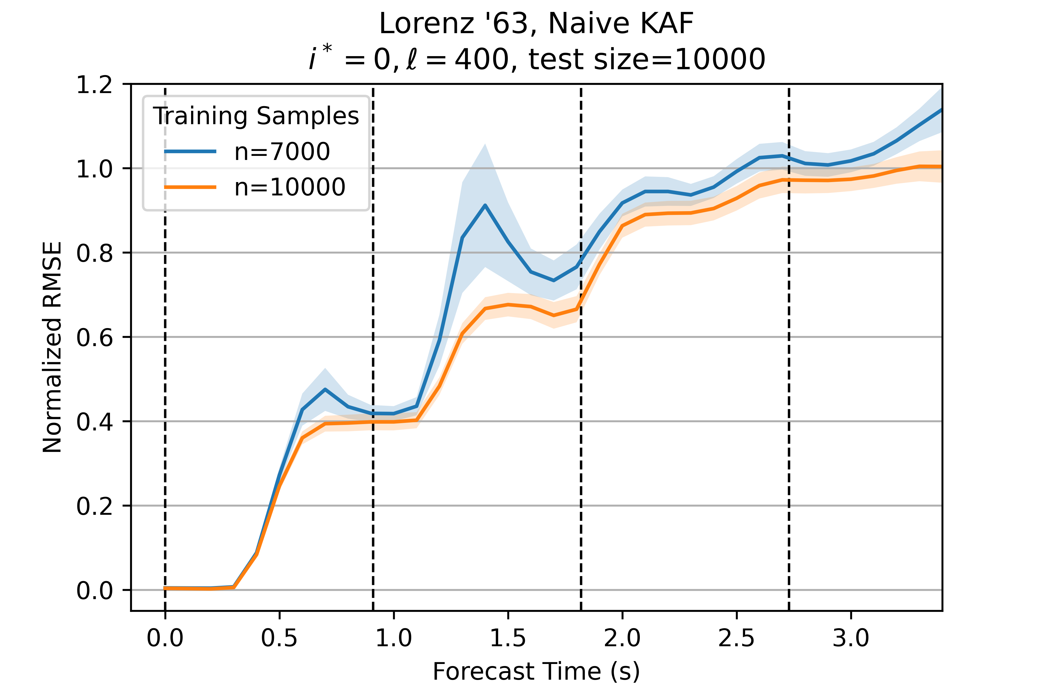
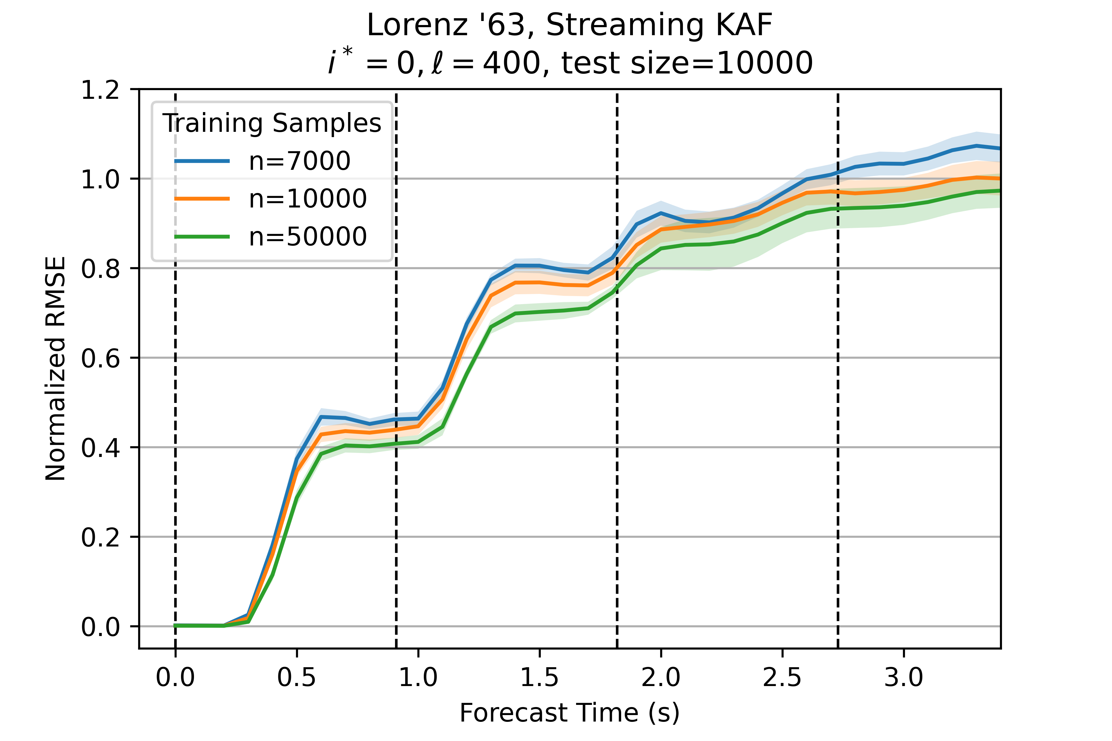
Figure 2: Lorenz ’63: Forecast error versus amount of training data. Average normalized RMSE for forecasting the first state variable of L63 via naïve KAF [left] and streaming KAF [right] as a function of the number $n$ of training points. The regression model has dimension $\ell=400$, the kernel inverse bandwidth $\gamma=.05$, and the number of features $s=\sqrt{n}\log(n)$. For $n=50,000$, naïve KAF fails because of its computational cost. See Section 4.4.

The KAF methodology has similar success at forecasting all three state variables. For each of the three variables and with $n=10,000$ training samples, Fig. 3 compares the forecasting error attained by the naïve and streaming methods.

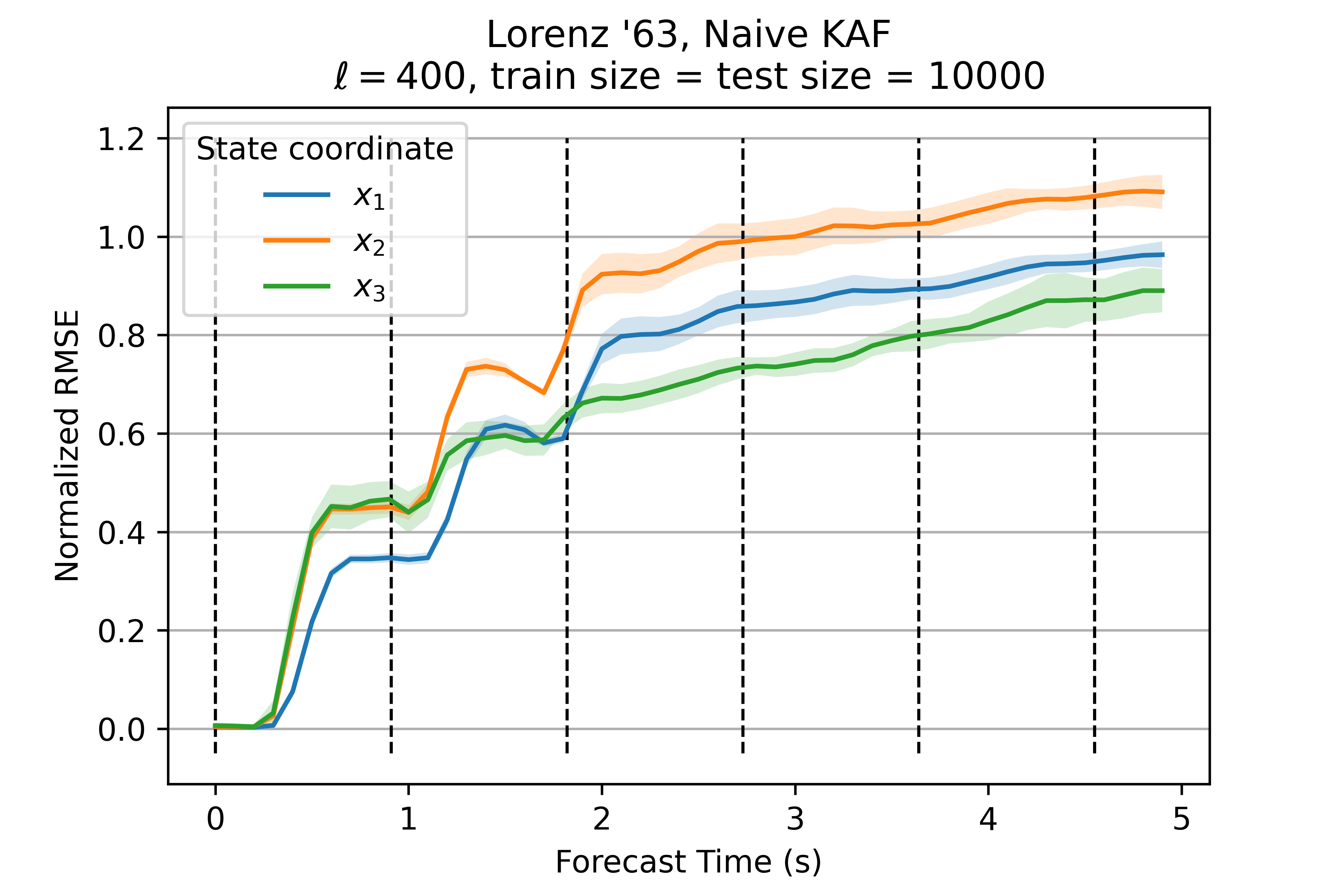
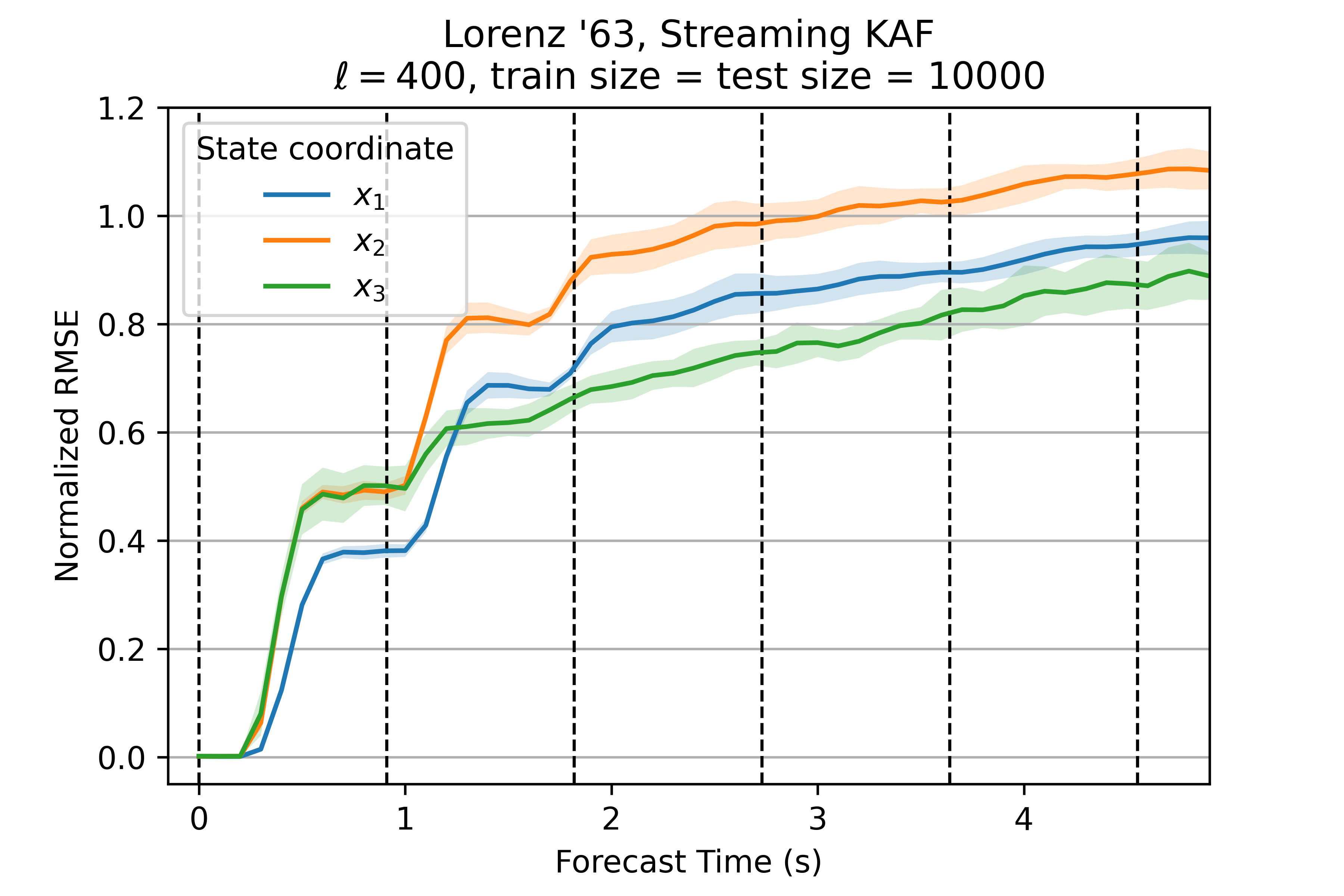
Figure 3: Lorenz ’63: Forecasting all three state variables. Average normalized RMSE for forecasting all three state coordinates $(x_{1},x_{2},x_{3})=(\text{blue, orange, green})$ via naïve KAF [left] and streaming KAF [right] with $n=10,000$ training points. The regression model has dimension $\ell=400$, the kernel inverse bandwidth $\gamma=.05$, and the number of features $s=\sqrt{n}\log(n)$. See Section 4.4.

4.5 Case Study: L96

In our second set of experiments, we explore the performance of scalable KAF for the L96 system in the periodic, quasi-periodic, and chaotic regimes documented in [13]. An increase in the forcing constant $F$ generates more chaotic behavior and, unsurprisingly, reduces the time horizon for which KAF can make informative forecasts.

For the periodic regime ($F=5$), forecasting is quite easy. Figure 4 illustrates the performance of streaming KAF as a function of the number $n$ of training samples. The success of the method hardly varies as we increase $n$ from $5,000$ to $20,000$, and the RMSE remains quite small over long time scales.

For the quasi-periodic regime ($F=6.9$), the forecasting problem becomes more challenging. For $n=10,000$ training samples, Fig. 5 shows that the naïve and streaming methods have similar forecasting performance for the first three slow variables. As we anticipate, the RMSE increases gradually with time. Figure 4 displays the performance of streaming KAF as a function of the number $n$ of training samples. In this case, an increase in the number of samples from $n=10,000$ to $n=50,000$ improves the performance moderately. Note that the naïve approach cannot benefit from the larger training set because it does not scale to input of this size.

Last, we consider the chaotic regime ($F=10$), where the forecasting problem is hard. Figure 6 indicates the naïve and streaming methods produce comparable forecasting results. In both cases, the RMSE increases quite quickly. Figure 4 shows that streaming KAF can build models from an increasing number $n$ of training samples, and it can attain an advantage from the larger training set.

We conclude that streaming KAF and naïve KAF have similar forecasting skill in all three regimes, even though the streaming method makes several approximations. At the same time, streaming KAF is far more economical, so it can exploit larger sets of training data and thereby construct more accurate models.

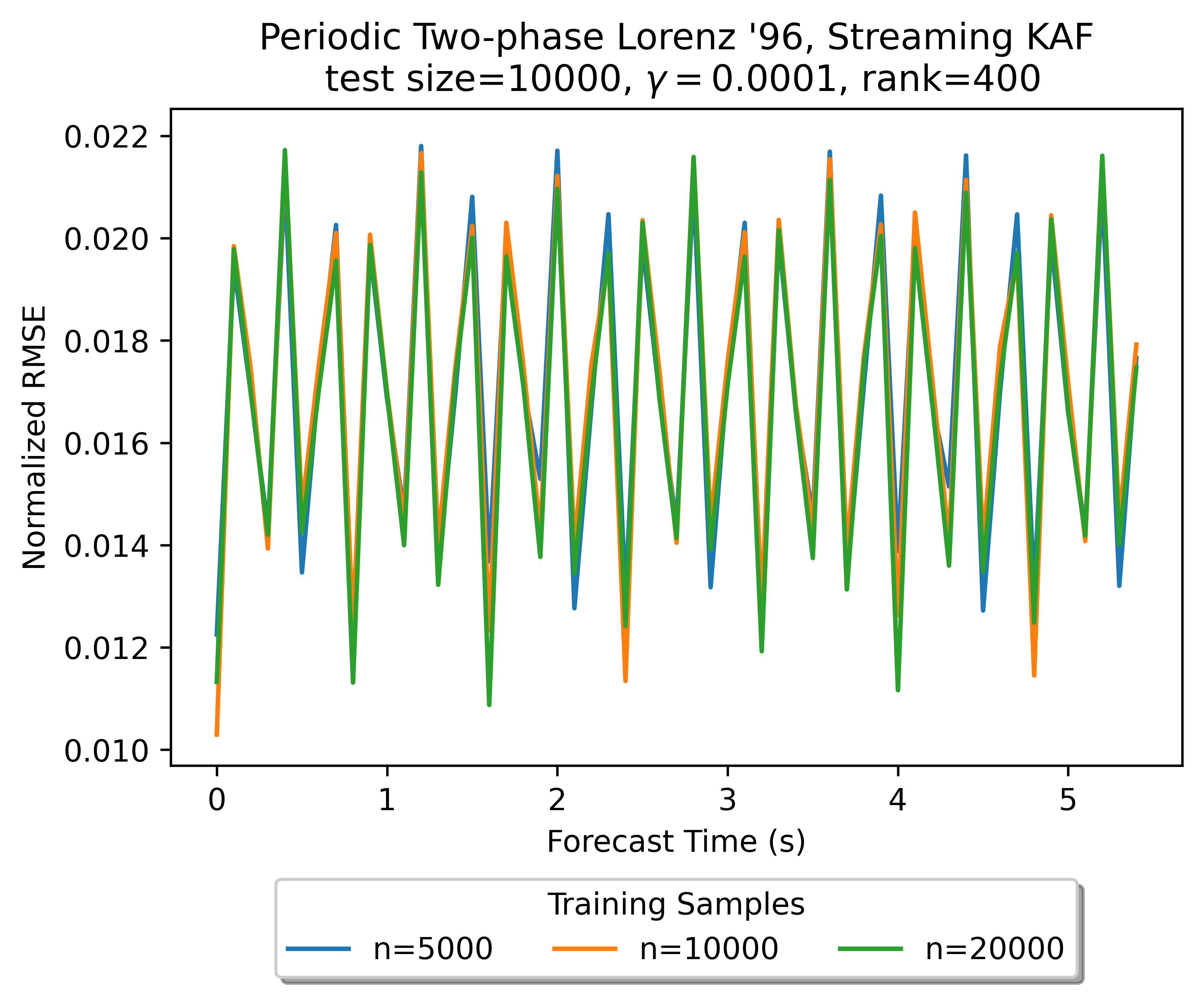
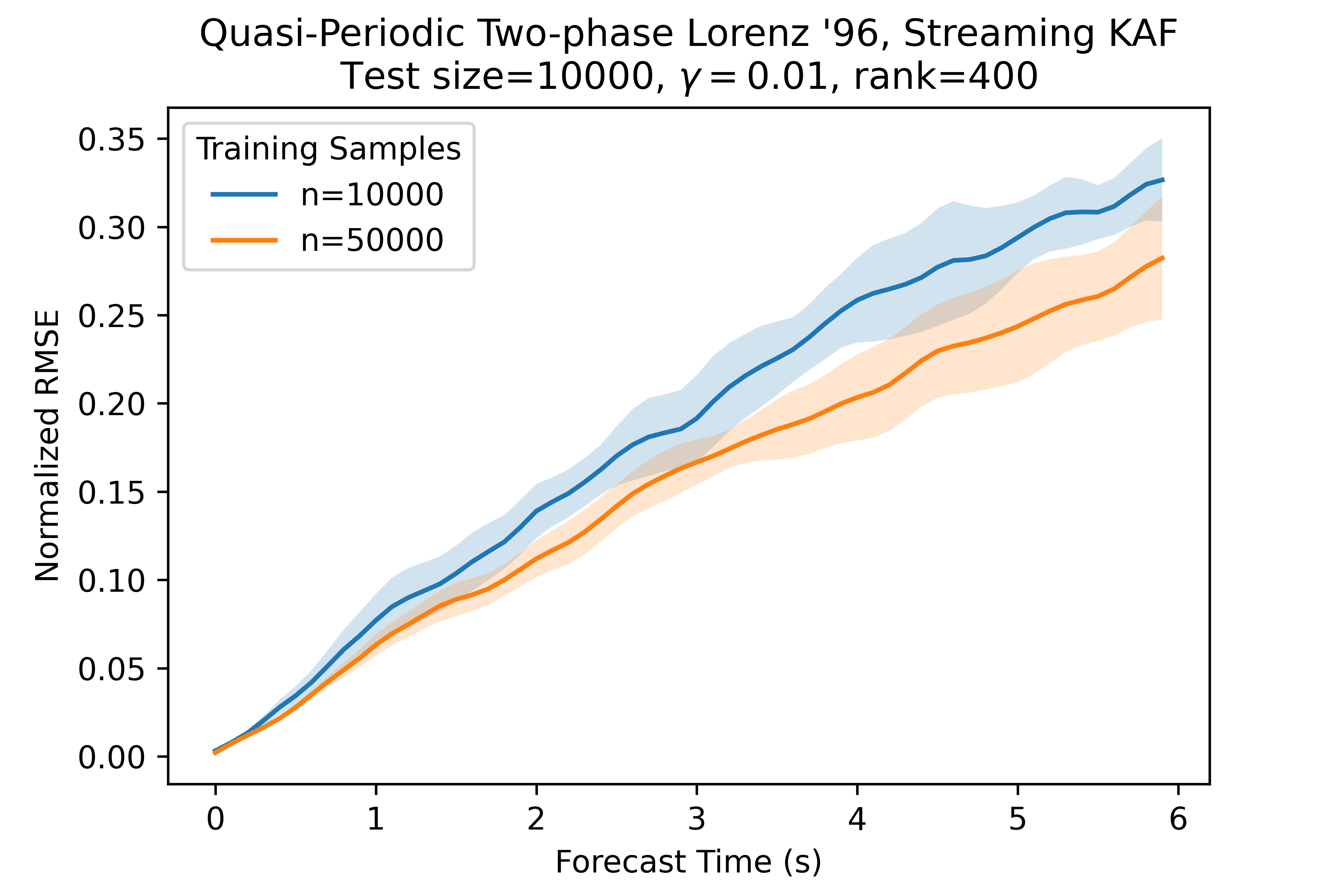
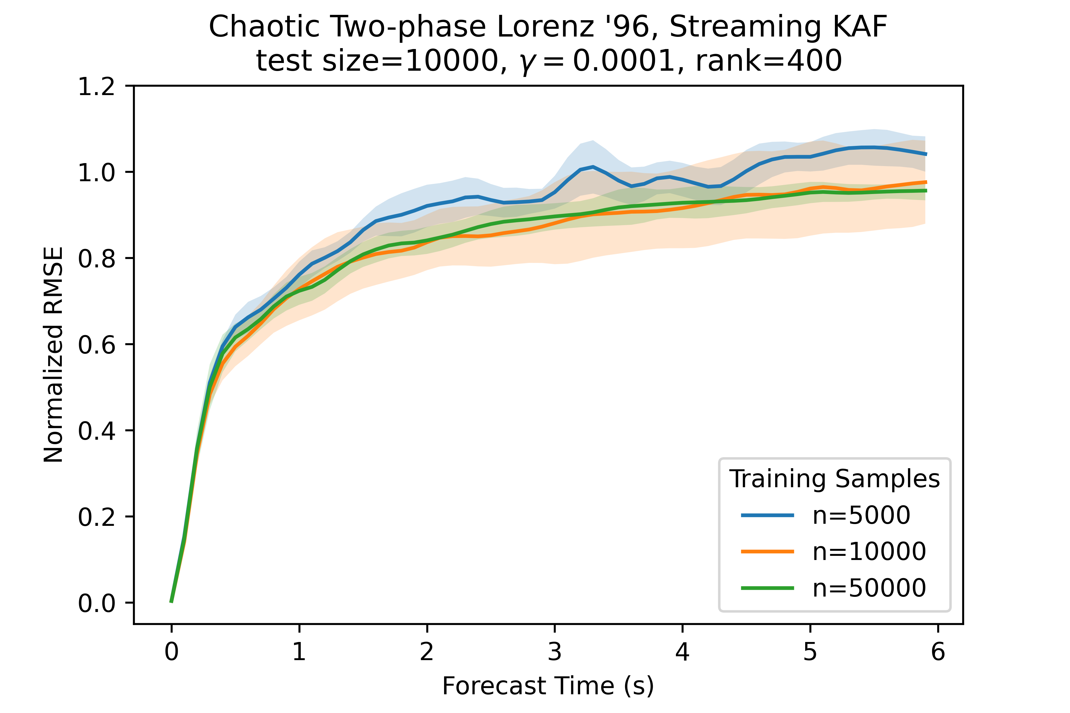
Figure 4: Lorenz ’96: Forecasting error versus amount of training data. Via streaming KAF, the average normalized RMSE for forecasting the first slow variable of periodic L96 [top], quasi-periodic L96 [bottom left], and chaotic L96 [bottom right] as a function of the number $n$ of training points. The regression model has dimension $\ell=400$, and the number of features $s=\sqrt{n}\log(n)$. The kernel inverse bandwidth $\gamma=0.0001$ in the periodic and chaotic cases, while $\gamma=0.01$ in the quasi-periodic case. See Section 4.5.

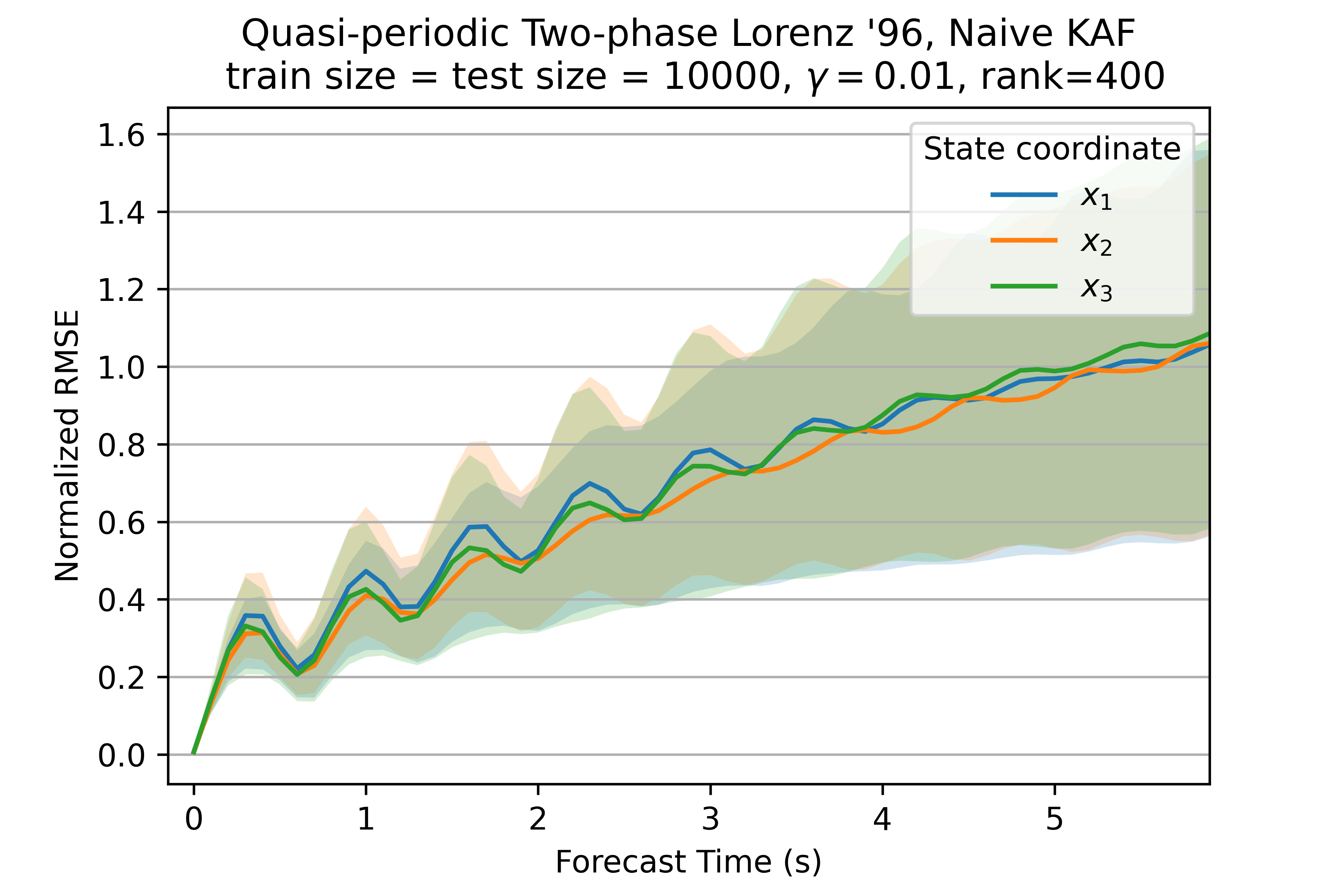
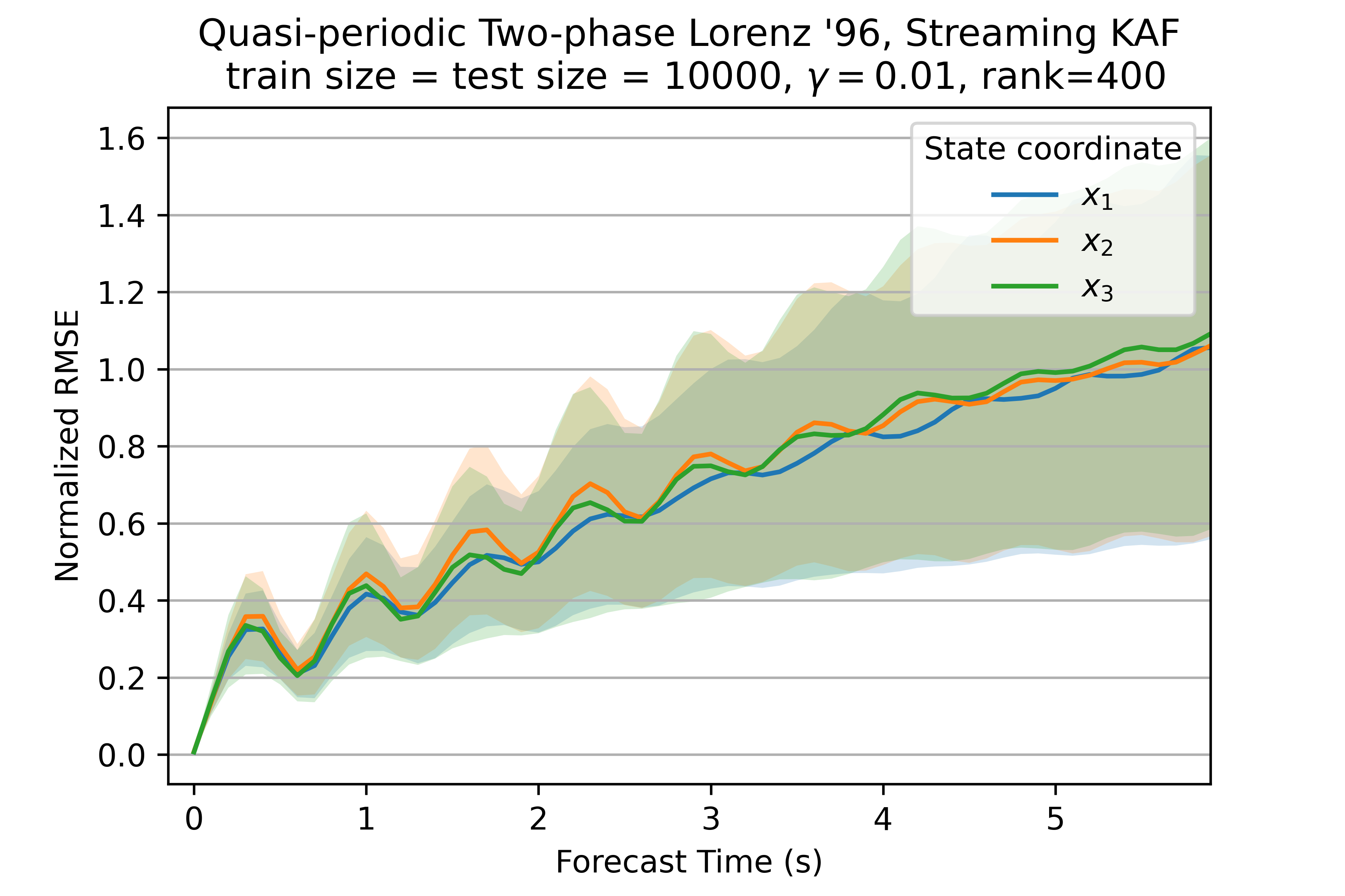
Figure 5: Quasi-periodic Lorenz ’96: Forecasting three slow variables. Average normalized RMSE for forecasting three slow coordinates $(x_{1},x_{2},x_{3})=(\text{blue, orange, green})$ of quasi-periodic L96 via naïve KAF [left] and streaming KAF [right] with $n=10,000$ training points. The regression model has dimension $\ell=400$, the kernel inverse bandwidth $\gamma=.0001$, and the number of features $s=\sqrt{n}\log(n)$. See Section 4.5.

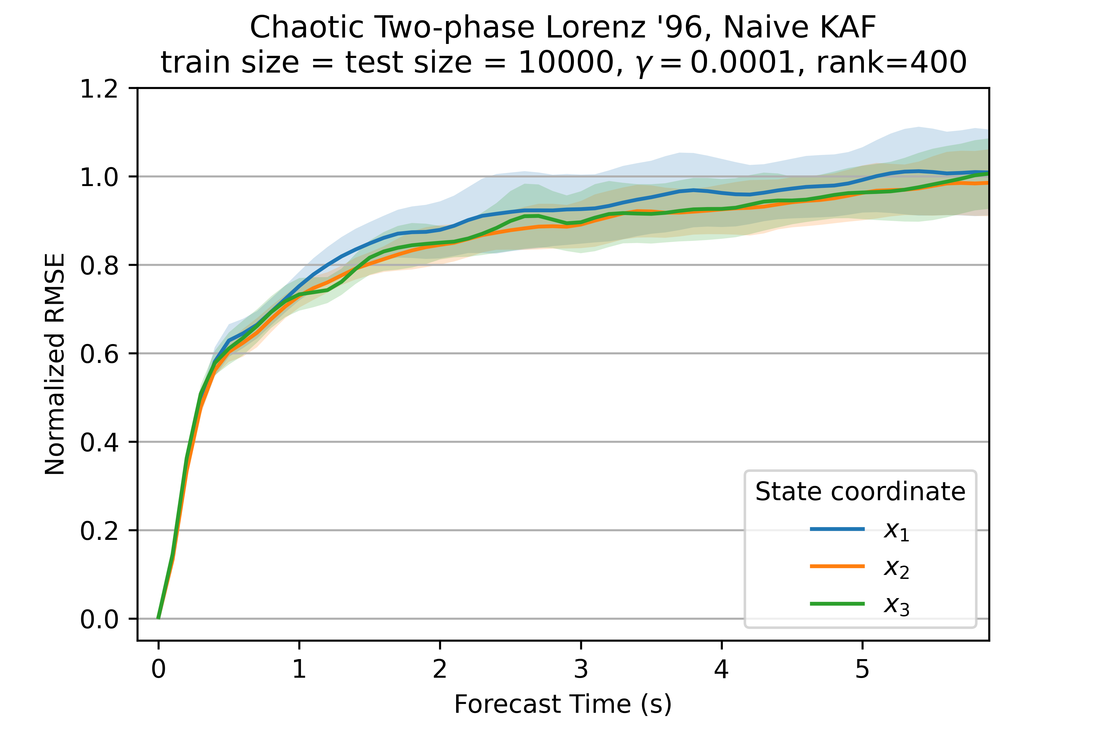
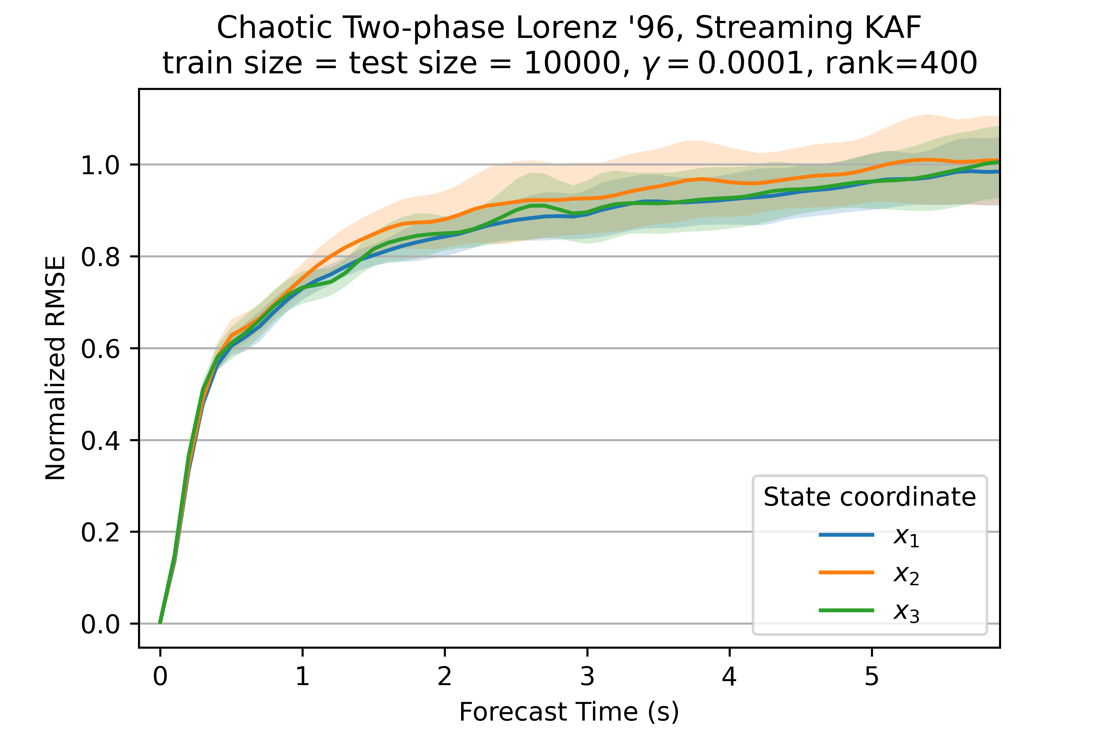
Figure 6: Chaotic Lorenz ’96: Forecasting three slow variables. Average normalized RMSE for forecasting three slow variables $(x_{1},x_{2},x_{3})=(\text{blue, orange, green})$ of chaotic L96 via naïve KAF [left] and streaming KAF [right] with $n=10,000$ training points. The regression model has dimension $\ell=400$, the kernel inverse bandwidth $\gamma=0.0001$, and the number of features $s=\sqrt{n}\log(n)$. See Section 4.5.

4.6 Hyperparameter specifications and sensitivity

The streaming KAF method involves several hyperparameters: the kernel inverse bandwidth $\gamma$, the dimension $\ell$ of the regression model, and the number $s$ of random features. We performed a collection of experiments with the L63 and L96 data to gauge how much the hyperparameters affect the quality of forecasts.

4.6.1 Kernel bandwidth

The inverse bandwidth parameter $\gamma$ of the Gaussian RBF kernel is a notorious hyperparameter that can have a significant impact on the performance of kernel methods. One basic methodology for selecting the bandwidth is the median rule [25], which sets $\gamma^{-1/2}$ to be the median pairwise distance among elements of a subsample from the dataset. Other quantiles of the pairwise distance, such as the 0.1 and 0.9 quantiles, are sometimes employed. A different approach for bandwidth tuning [16] leverages scaling relationships between the element sum of the $n\times n$ kernel matrix $\bm{K}_{x,x}$ and $\gamma$.

In our experience, the KAF methodology is robust to the choice of inverse bandwidth parameter in all problem regimes. Indeed, the forecasting performance is similar over several orders of magnitude, but tuning can have a modest effect. See Fig. 7 for an illustration. To obtain better models from large training data, we invoke scaling laws for the bandwidth.

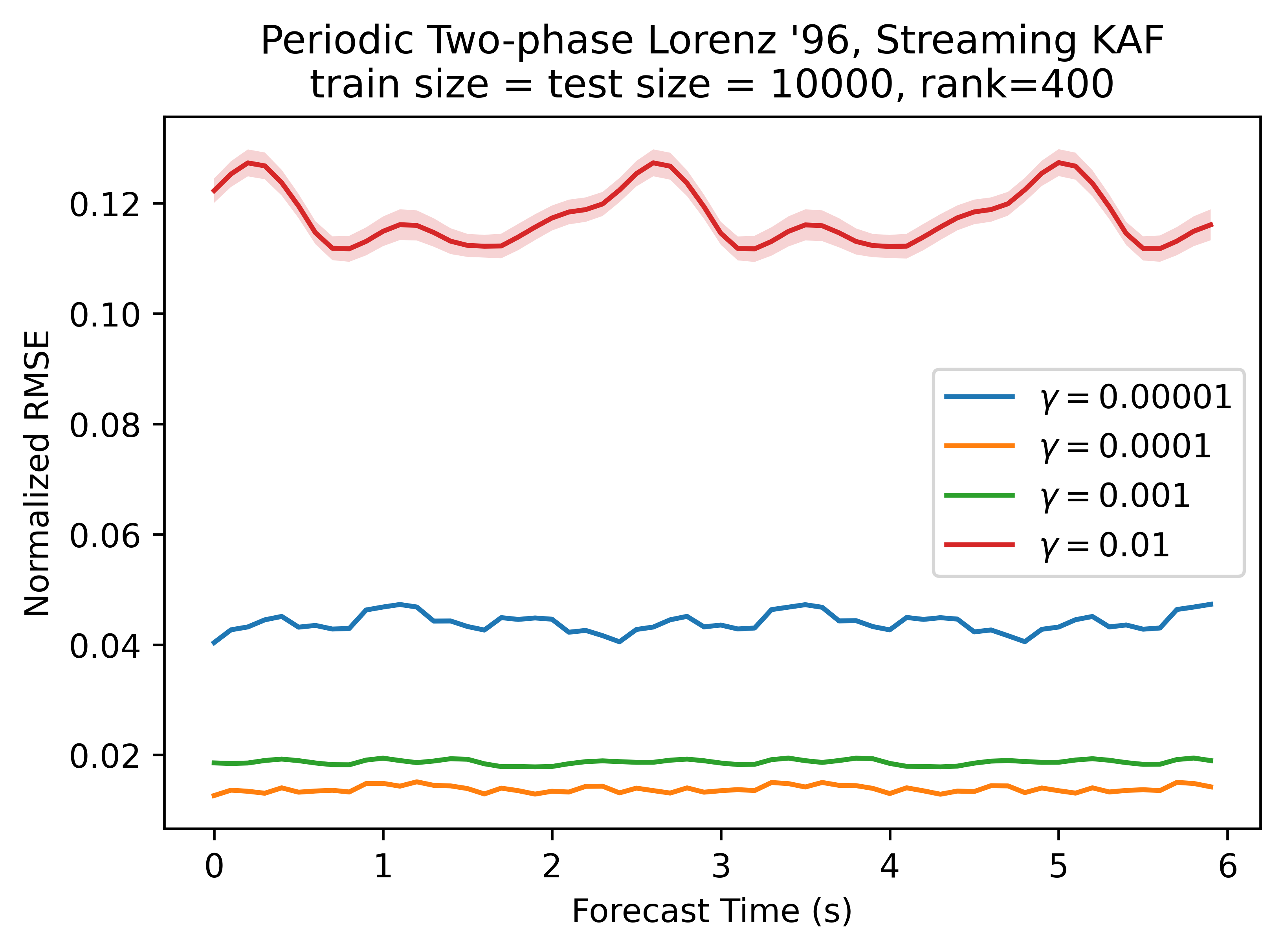
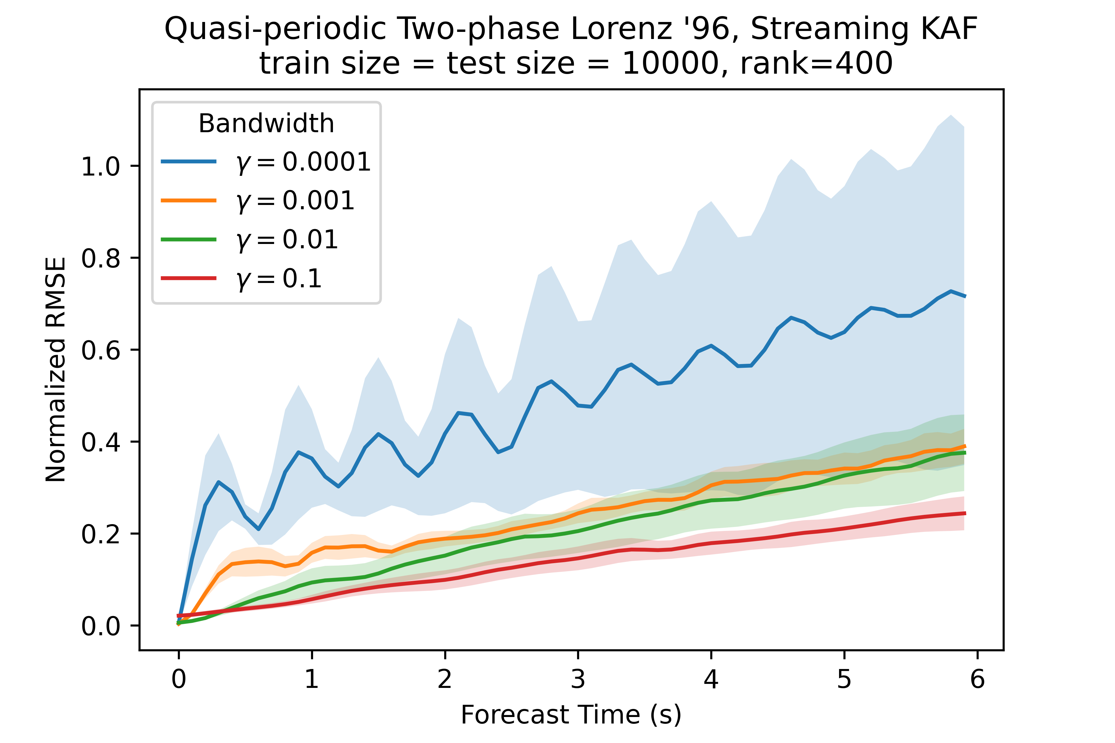
Figure 7: Robustness to inverse bandwidth parameter: For the L96 system in the periodic regime [left] and the quasi-periodic regime [right], the quality of the forecast is robust to the choice of $\gamma$. In each case, we use $n=10,000$ training samples, and the regression model has dimension $\ell=400$. See Section 4.6.1.

4.6.2 Dimension of regression model

To implement streaming KAF, we must choose the dimension, or rank, $\ell$ of the regression model. When $\ell$ is too small, the model does not capture all of the dynamics. Meanwhile, when $\ell$ is too large, we can introduce noise dimensions or encounter numerical problems. In this section, we outline some strategies for this task, and we will show that the forecasting methodology is robust to the choice of this parameter.

One principled approach is to form the full covariance matrix $\bm{C}_{xx}\in\mathbbm{R}^{s\times s}$ or $\bm{C}_{uu}\in\mathbbm{R}^{s\times s}$ of the covariate data. In this case, we can explicitly compute the eigenvalues $(\lambda_{1},\lambda_{2},\dots,\lambda_{s})$ of the matrix. Then, we choose the truncation level $\ell$ so that we capture, say, $99.9\%$ of the spectral content:

(22) $$\ell=\min\left\{k\in\mathbb{N}:\sum\nolimits_{i=1}^{k}\lambda_{i}\geq 0.999\cdot\sum\nolimits_{i=1}^{s}\lambda_{i}\right\}.$$

This method is effective for a range of problems. At the same time, it imposes additional computational costs, and it is not compatible with the streaming algorithm.

Instead, we typically prescribe the dimension $\ell$ of the regression model in advance using prior knowledge about the problem or to work within our computational budget. For example, in our medium-scale experiments, we make the choice $\ell=400$, which captures over $99.9\%$ of the spectral content of the computed covariance matrices. Since we have included the ridge regularization $\mu\mathbf{I}$ in the forecasting function, we can insulate the algorithm from the negative impact of outsize $\ell$.

Given a conservative (i.e., large) initial value of $\ell$, randomized Nyström produces an estimate for the first $\ell$ eigenvalues of the covariance matrix. Using this estimate, we can apply the rule Eq. 22 a posteriori to further reduce the dimension of the regression model. This is often a good compromise, but further research on principled methods would be valuable.

Regardless, our numerical experiments indicate that streaming KAF forecast is somewhat insensitive to the dimension $\ell$ of the regression model. See Fig. 8 for some evidence. For large training data sets, we scale up the dimension $\ell$ to obtain more accurate forecasts.

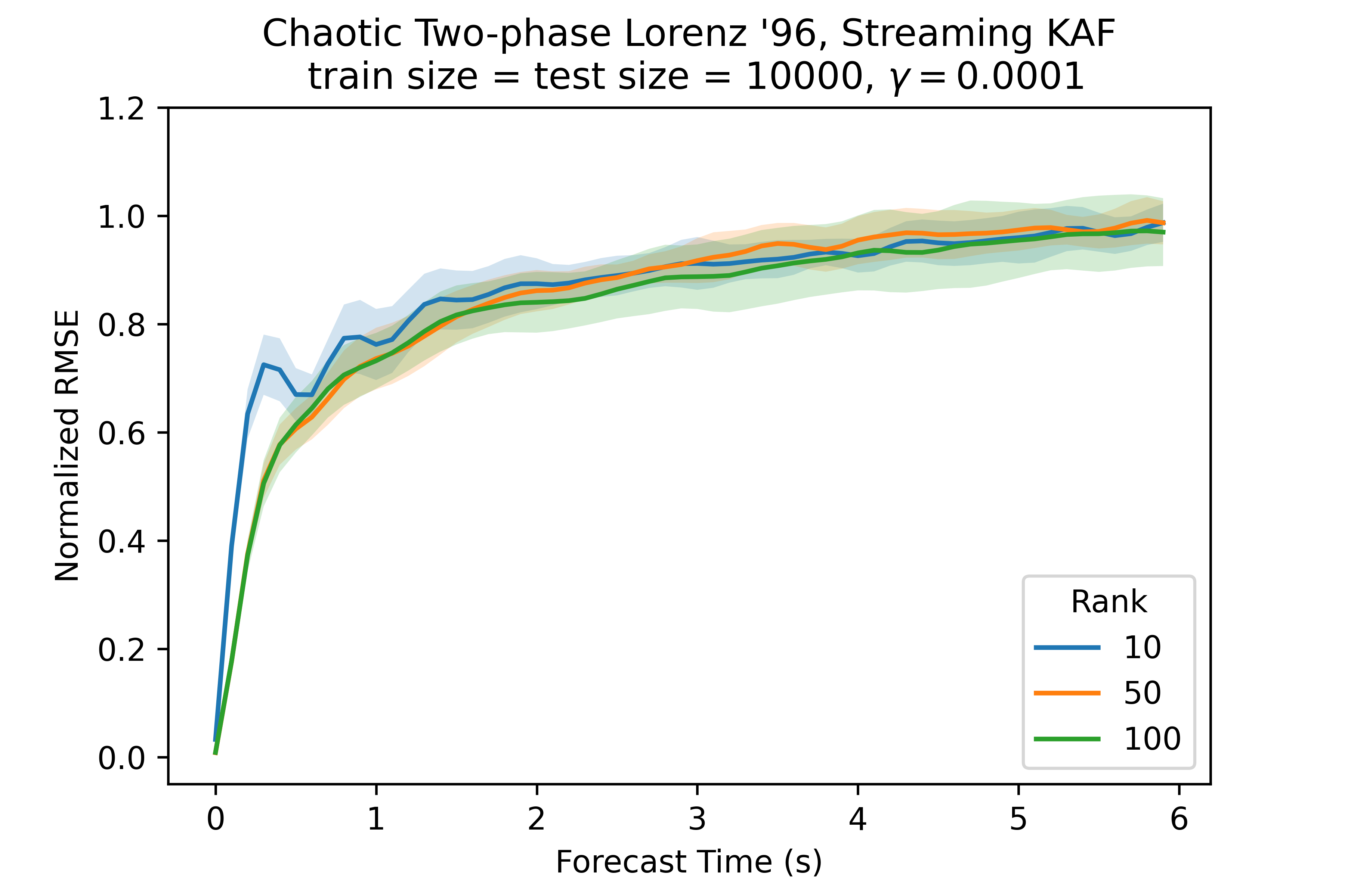
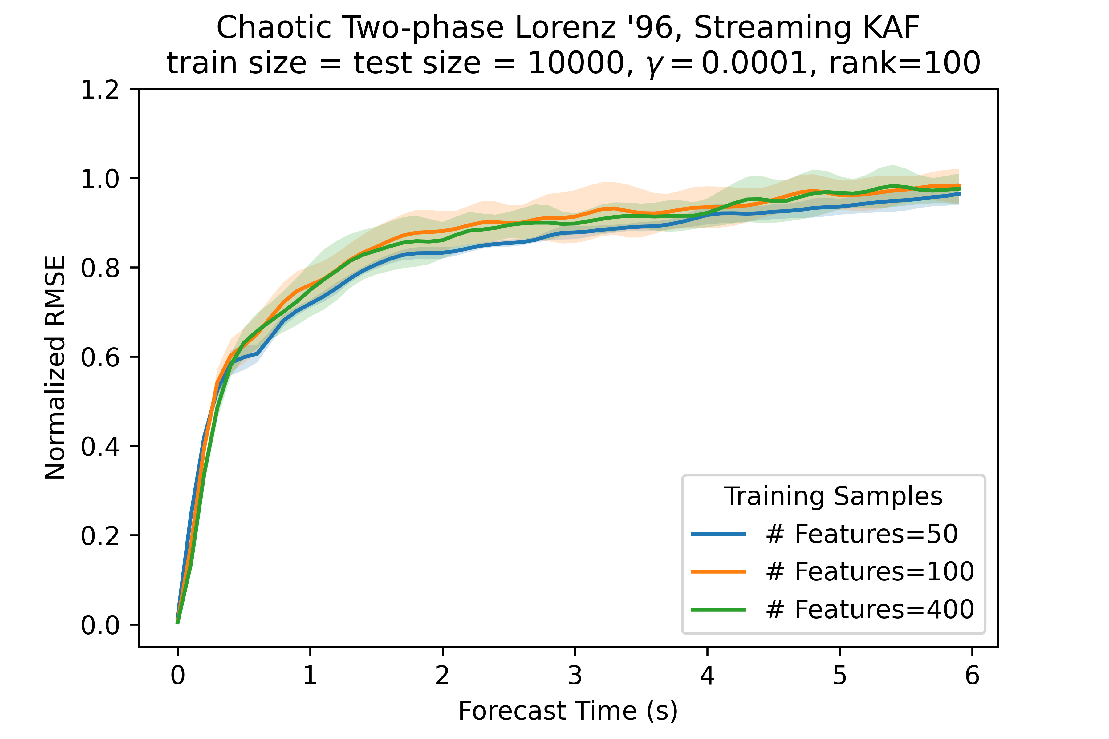
Figure 8: Robustness to dimension of regression model and number of random features. For the L96 system in the chaotic regime, the quality of the forecast is robust to the dimension $\ell$ of the regression model [left] and to the number $s$ of random features [right]. In the left panel, $s=100$. In the right panel, $\ell=100$. In each case, we use $n=10,000$ training samples, and the kernel inverse bandwidth $\gamma=0.0001$. See Sections 4.6.2 and 4.6.3.

4.6.3 Number of random features

The last parameter in the streaming KAF algorithm is the number $s$ of random features that we use to approximate the kernel function. As discussed in Section 3.3, the choice $s=\sqrt{n}\log(n)$ is theoretically justified for kernel regression in a statistical setting. In the majority of our experiments, we adopt the value $s=\sqrt{n}\log(n)$, and we have found that the streaming KAF method always performs well. Furthermore, taking a larger number of random features does not seem to offer any further benefit, and taking fewer random features is not detrimental. See Fig. 8 for evidence.

In the streaming setting, we may not know the number $n$ of training points in advance and we do not want the model size to depend on the amount of input data, so the prescription $s=\sqrt{n}\log(n)$ might be unappealing. Our computational work supports the recommendation that the number $s$ of random features may be a small integer multiple of the dimension $\ell$ of the regression model. It would be interesting to understand this phenomenon better from both an empirical and a theoretical point of view.

Table 2: L63: Timing costs and error in forecasting. This table reports the time cost (in seconds) required to construct and evaluate a forecasting model using Streaming and Naïve KAF algorithms, along with the average normalized RMSE of the resulting models. The covariate is the $3$-dimensional state of the L63 system, and the response is the first state variable after $0.5$ time units. The number $n$ of training samples varies, and the number of random features $s=\sqrt{n}\log(n)$. Reported test time is for making all $m=10,000$ forecasts. See Section 4.7 for more details.

		$(1e4,4e2,.09)$	$(5e4,8e2,.18)$	$(1e5,12e2,.27)$	$(5e5,16e2,.36)$	(1e6, 24e2, .54)	(5e6, 32e2, .72)
Train	Streaming	.565	6.739	29.025	387.265	1588.570	26390.902
	Naïve	58.684	—	—	—	—	—
Test	Streaming	.047	.163	.267	.723	.936	2.703
	Naïve	15.311	—	—	—	—	—
RMSE	Streaming	.262	.177	.170	.107	.065	.047
	Naïve	.228	—	—	—	—	—

Table 3: L63: Timing costs and error in forecasting using fewer random features. This table reports the time cost (in seconds) required to construct and evaluate a forecasting model using Streaming KAF. The setup is the same as in Table 2, but with model parameters $(s,\ell,\gamma)=(3200,3200,.72)$ fixed for all experiments. See Section 4.7 for more details.

	$\bm{n=1e4}$	5e4	1e5	5e5	1e6	5e6
Train	35.101	43.051	55.079	138.083	253.435	1061.187
Test	.230	.220	.245	.229	.221	.219
RMSE	.408	.125	.119	.086	.075	.089

4.7 Timing comparisons

We have demonstrated that streaming KAF constructs accurate forecasting models in a range of scenarios. Therefore, we may turn our attention to the computational costs of training and forecasting. Table 2 compares the runtimes of naïve KAF and streaming KAF, and it charts the average normalized RMSE of the resulting models.

These experiments are based on the L63 data. We forecast the first state variable from the full set of three state variables. The forecast horizon is fixed at $q=0.5$ time units. The number $n$ of training samples varies, while the number of test samples remains fixed at $m=10,000$. The kernel inverse bandwidth $\gamma=0.09$, and the dimension of the regression model grows from $\ell=400$ to $\ell=3200$ in rough proportion to $\log n$. For the streaming method, the number of random features $s=\sqrt{n}\log(n)$ also increases with the size of the training data. We report the average RMSE over five test runs.

To be clear, the training time includes the full cost of computing the weight matrix $\check{\bm{W}}_{q,\ell}$ for a single real-valued response at a single forecast horizon $q$. This cost includes the evaluation of random features, formation of the covariance matrices, the streaming PCA computation, and the matrix product. For making a forecast, the timing reflects the full cost of computing $m=10,000$ real-valued responses for the fixed time horizon $q$, including the evaluation of random features and the matrix product.

For small problems, we see that the training time for streaming KAF is 100–200$\times$ faster than naïve KAF. The test time for streaming KAF is 300–400$\times$ faster, and the models achieve similar RMSE. For large problems, naïve KAF is unable to produce a forecasting model. Meanwhile, streaming KAF can build a forecasting model from $n=5\cdot 10^{6}$ training samples in less than two hours on a laptop, and this model can produce a single real-valued forecast in about $0.0003\mathrm{s}$. As the amount of training data increases, the RMSE of the forecasting models continues to improve, which underscores how important it is to develop a scalable algorithm.

Out of a sense of fair play, we used the theoretically supported number $s=\sqrt{n}\log(n)$ of random features. If we adopt our empirical recommendation $s=\mathrm{Const}\cdot\ell$, the timings improve markedly without sacrificing much accuracy. Table 3 displays the runtimes and average normalized RMSE for streaming KAF under the same experimental set-up as in Table 2, but with the regression dimension and number of random features fixed at $(\ell,s)=(3200,3200)$. The user may judge whether the speedup warrants the modest loss in RMSE.

5 Comparison with related work

Several other techniques for data-driven prediction have been proposed and studied recently. Here, we comment on the mathematical and computational characteristics of these approaches in relation to streaming KAF, focusing on methods that employ aspects of linear operator theory or randomized linear algebra. Within this context, forecasting techniques can be broadly classified as reduced modeling approaches (i.e., methods that construct a surrogate dynamical system from observed data) and regression approaches (i.e., supervised learning techniques for estimating covariate–response relationships).

5.1 Forecasting methodologies

Examples of reduced modeling techniques are linear inverse models [66], (extended) DMD [70, 73, 84], and methods for approximating the Koopman generator [28, 19, 46]. These methods formally assume that the training data have a (deterministic) Markovian evolution. That assumption is clearly satisfied under the autonomous dynamics in (1) if the training data are snapshots $\bm{x}_{0},\bm{x}_{1},\ldots$ of the full system state in $\mathbb{R}^{d}$. On the other hand, if we have access to samples $u(\bm{x}_{0}),u(\bm{x}_{1}),\ldots$ of a covariate $u:\mathbb{R}^{d}\to\mathbb{R}^{d^{\prime}}$ with $d^{\prime}<d$, then training data are generally non-Markovian (unless $u$ happens to lie in a Koopman-invariant subspace). Approaches for overcoming non-Markovianity include dimension augmentation through delay-coordinate maps [72, 12, 30] and incorporation of memory terms using the Mori-Zwanzig formalism [33, 35].

Other approaches model the observed data as realizations of a stochastic process. For example, techniques based on Ulam’s method [20, 44] estimate the transfer operator of a dynamical system (which is a dual operator to the Koopman operator, acting on probability measures) in a basis of indicator functions associated with a partition of state space. The diffusion forecasting technique [8] estimates the evolution semigroup associated with a stochastic differential equation (SDE) on a manifold in a smooth data-driven basis of kernel eigenfunctions learned through the diffusion maps algorithm [15]. Extensions of DMD to random dynamical systems [18] and SDEs [3] have also been proposed recently.

A common aspect of reduced modeling techniques is that they learn a surrogate model of the dynamics from time series data. Often, in order to make a forecast to a horizon of $q$ time units, these models are trained on a shorter timestep $q^{\prime}<q$ and iteratively applied $q/q^{\prime}$ times to reach the desired horizon. This approach is attractive because it allows simulation of the long-term statistical behavior of the system (assuming that the training phase was successful).

In contrast, regression-based methodologies usually operate by constructing a forecast function at a fixed lead time (or a family of independent forecast functions up to a desired lead time), and they evaluate the forecast once on the initial data to yield a prediction. This approach offers greater generality than reduced modeling approaches, since Markovianity of the covariate–response observables is not required, nor is it required that the covariate and response lie in a Koopman-invariant subspace [30]. Indeed, as discussed in Section 2.7, KAF yields asymptotically optimal predictions (in the $L_{2}$ or RMSE sense) in the large-data limit in the form of the conditional expectation of the Koopman-evolved response conditioned on the covariate. Yet, at the same time, the conditional expectation may not be a good approximation for actual dynamical trajectories, which makes direct regression approaches unsuitable for simulating the statistical behavior of the system (despite yielding RMSE-optimal forecasts). For further details, see the paper [13], which studies applications of KAF to multiscale systems with averaging and homogenization limits. A recent paper [38] has explored applications of kernel learning [63] to forecasting with kernel regression.

All of the above approaches are purely data-driven, in the sense that they only use time-ordered data snapshots as inputs, without requiring knowledge of the equations of motion. Yet, in many applications, full or partial knowledge of the equations of motion is available, and it is natural to design methods that take advantage of that knowledge [37]. An example is the “lift and learn” framework [67] which employs a mapping to transport the data to a higher-dimensional space where the system is quadratic. Unlike the Koopman operator, the existence of a finite-dimensional quadratic representation of the system dynamics is not universally guaranteed, but can be constructed for many systems encountered in physical and engineering applications [34] if the equations of motion are known. The approach of [67] leverages the quadratic structure of the system in the lifted space by employing a projection that is compatible with quadratic nonlinearities (see also [65]). In this manner, the reduced model is compatible with the “physics” of the lifted model. In [67], the projection is obtained from the proper orthogonal decomposition (POD) [42], which computes a low-rank approximation to the autocorrelation matrix $\bm{X}\bm{X}^{\top}\in\mathbb{R}^{d\times d}$ rather than the covariance matrix $\bm{X}^{\top}\bm{X}\in\mathbb{R}^{n\times n}$. The randomized singular value decomposition is also used within this forecasting framework to build a scalable implementation [58].

Note that the eigenvectors of $\bm{X}\bm{X}^{\top}$ are spatial vectors in $\mathbb{R}^{d}$. In DMD, the analogous objects are the eigenvectors of the matrix $\bm{A}$ in (5), called Koopman modes [70], which can also be employed for model reduction. The KAF approach can be thought of as being “dual” to these methods in that it employs $n\times n$ kernel matrices which are discretizations of operators acting on spaces of observables of the system (rather than spatial patterns in $\mathbb{R}^{d}$).

5.2 Streaming algorithms for kernel computation

The machine learning literature contains a substantial body of work on kernel methods, techniques for combining kernels with random features, and methods for implementing these algorithms in a streaming setting. This space is not adequate for a comprehensive summary of this vast field. We recommend the book [74] as a foundational reference on kernel methods in machine learning.

The RFF technique [69] was developed to accelerate kernel computations. There are a substantial number of papers that use RFF for KRR, such as [5, 71], but we are not aware of a paper that uses random features for streaming kernel regression.

There are also several papers that combine RFF with streaming PCA algorithms to obtain streaming KPCA algorithms. In particular, Ghashami et al. [27] apply the frequent directions method [26], while Ullah et al. [81] use Oja’s algorithm [62]. Henriksen & Ward [41] have developed an adaptive extension of Oja’s algorithm that is significantly more robust. Tropp and coauthors have proposed to use the randomized Nyström method for streaming PCA [78], perhaps in combination with random features [57, Sec. 19.3.5]. Our numerical work suggests that the Nyström method is more accurate and more reliable than the alternatives in the context of streaming KAF.

We have also investigated the performance of streaming KAF using AdaOja [41] for the streaming PCA computation. In our experience, this approach can be competitive, especially in cases where the spectrum of the covariance matrix decays slowly. See [40] for a detailed report.

6 Conclusions

Kernel analog forecasting is a regression-based approach to forecasting dynamical systems that offers a theoretical guarantee of asymptotically optimal predictions (in the $L_{2}$ or RMSE sense) in the large-data limit. By incorporating two randomized approximation techniques from numerical linear algebra—random Fourier features and the randomized Nyström method—we developed a streaming implementation of kernel analog forecasting. This approach makes it possible to build forecasting models from large data sets where the KAF methodology is theoretically justified. Our experiments indicate that streaming KAF has the potential to unlock the promise of KAF as a general data-driven, non-parametric tool for making predictions of dynamical systems.

References

- [1] R. Alexander and D. Giannakis, Operator-theoretic framework for forecasting nonlinear time series with kernel analog techniques, Physica D: Nonlinear Phenomena, 409 (2020), p. 132520, https://doi.org/https://doi.org/10.1016/j.physd.2020.132520, https://www.sciencedirect.com/science/article/pii/S016727891930377X.
- [2] R. Alexander, Z. Zhao, E. Székely, and D. Giannakis, Kernel analog forecasting of tropical intraseasonal oscillations, Journal of Atmospheric Sciences, 74 (2017), pp. 1321–1342.
- [3] H. Arbabi and T. Sapsis, Generative stochastic modeling of strongly nonlinear flows with non-Gaussian statistics, 2021, https://arxiv.org/abs/1908.08941.
- [4] N. Aronszajn, Theory of reproducing kernels, Trans. Amer. Math. Soc., 68 (1950), pp. 337–404, https://doi.org/10.2307/1990404, https://doi-org.clsproxy.library.caltech.edu/10.2307/1990404.
- [5] H. Avron, M. Kapralov, C. Musco, C. Musco, A. Velingker, and A. Zandieh, Random Fourier features for kernel ridge regression: Approximation bounds and statistical guarantees, in Proceedings of the 34th International Conference on Machine Learning, vol. 70 of Proceedings of Machine Learning Research, 06–11 Aug 2017, pp. 253–262.
- [6] V. Baladi, Positive Transfer Operators and Decay of Correlations, vol. 16 of Advanced Series in Nonlinear Dynamics, World scientific, Singapore, 2000.
- [7] M. Belkin, Approximation beats concentration? an approximation view on inference with smooth radial kernels, in Conference On Learning Theory, PMLR, 2018, pp. 1348–1361.
- [8] T. Berry, D. Giannakis, and J. Harlim, Nonparametric forecasting of low-dimensional dynamical systems, Phys. Rev. E., 91 (2015), p. 032915, https://doi.org/10.1103/PhysRevE.91.032915.
- [9] T. Berry, D. Giannakis, and J. Harlim, Bridging data science and dynamical systems theory, Notices Amer. Math. Soc., 67 (2020), pp. 1336–1349, https://doi.org/10.1090/noti2151.
- [10] Å. Björck, Numerical methods for least squares problems, SIAM, 1996.
- [11] S. S. Bochner, Vorlesungen über Fouriersche Integrale von S. Bochner., Mathematik und ihre Anwendungen in Monographien und Lehrbüchern ; Bd. 12, Akademische Verlagsgesellschaft, Leipzig, 1932.
- [12] S. L. Brunton, B. W. Brunton, J. L. Proctor, E. Kaiser, and J. N. Kutz, Chaos as an intermittently forced linear system, Nat. Commun., 8 (2017), https://doi.org/10.1038/s41467-017-00030-8.
- [13] D. Burov, D. Giannakis, K. Manohar, and A. Stuart, Kernel analog forecasting: Multiscale test problems, Multiscale Model. Simul., 19 (2021), pp. 1011–1040, https://doi.org/10.1137/20M1338289.
- [14] Y. Cherapanamjeri and J. Nelson, Uniform distribution approximation for randomized hadamard transforms with applications, preprint, (2021).
- [15] R. R. Coifman and S. Lafon, Diffusion maps, Appl. Comput. Harmon. Anal., 21 (2006), pp. 5–30, https://doi.org/10.1016/j.acha.2006.04.006.
- [16] R. R. Coifman, Y. Shkolnisky, F. J. Sigworth, and A. Singer, Graph Laplacian tomography from unknown random projections, IEEE Trans. Image Process., 17 (2008), pp. 1891–1899, https://doi.org/10.1109/tip.2008.2002305.
- [17] D. Comeau, Z. Zhao, D. Giannakis, and A. J. Majda, Data-driven prediction strategies for low-frequency patterns of north pacific climate variability, Climate Dynamics, 48 (2017), pp. 1855–1872.
- [18] N. Cřnjarić-Žic, S. Maćešić, and I. Mezić, Koopman operator spectrum for random dynamical systems, J. Nonlinear Sci., 30 (2020), pp. 2007–2056, https://doi.org/10.1007/s00332-019-09582-z.
- [19] S. Das, D. Giannakis, and J. Slawinska, Reproducing kernel Hilbert space quantification of unitary evolution groups, Appl. Comput. Harmon. Anal., 54 (2021), pp. 75–136, https://doi.org/10.1016/j.acha.2021.02.004.
- [20] M. Dellnitz and O. Junge, On the approximation of complicated dynamical behavior, SIAM J. Numer. Anal., 36 (1999), p. 491, https://doi.org/10.1137/S0036142996313002.
- [21] T. Eisner, B. Farkas, M. Haase, and R. Nagel, Operator Theoretic Aspects of Ergodic Theory, vol. 272 of Graduate Texts in Mathematics, Springer, 2015.
- [22] I. Fatkullin and E. Vanden-Eijnden, A computational strategy for multiscale systems with applications to lorenz 96 model, Journal of Computational Physics, 200 (2004), pp. 605–638.
- [23] I. Fatkullin and E. Vanden-Eijnden, A computational strategy for multiscale systems with applications to lorenz 96 model, Journal of Computational Physics, 200 (2004), pp. 605–638.
- [24] G. Froyland, G. A. Gottwald, and A. Hammerlindl, A computational method to extract macroscopic variables and their dynamics in multiscale systems, SIAM J. Appl. Dyn. Sys., 13 (2014), pp. 1816–1846, https://doi.org/10.1137/130943637.
- [25] D. Garreau, W. Jitkrittum, and M. Kanagawa, Large sample analysis of the median heuristic, arXiv preprint arXiv:1707.07269, (2017).
- [26] M. Ghashami, E. Liberty, J. M. Phillips, and D. P. Woodruff, Frequent directions: simple and deterministic matrix sketching, SIAM J. Comput., 45 (2016), pp. 1762–1792.
- [27] M. Ghashami, D. J. Perry, and J. Phillips, Streaming kernel principal component analysis, in Artificial intelligence and statistics, PMLR, 2016, pp. 1365–1374.
- [28] D. Giannakis, Data-driven spectral decomposition and forecasting of ergodic dynamical systems, Appl. Comput. Harmon. Anal., 62 (2019), pp. 338–396, https://doi.org/10.1016/j.acha.2017.09.001.
- [29] D. Giannakis, Delay-coordinate maps, coherence, and approximate spectra of evolution operators, Res. Math. Sci., 8 (2021), p. 8, https://doi.org/10.1007/s40687-020-00239-y.
- [30] F. Gilani, D. Giannakis, and J. Harlim, Kernel-based prediction of non-Markovian time series., Phys. D, 418 (2020), p. 132829, https://doi.org/10.1016/j.physd.2020.132829.
- [31] A. Gittens, Topics in Randomized Numerical Linear Algebra, 2013. Thesis (Ph.D.)–California Institute of Technology.
- [32] G. H. Golub and C. F. Van Loan, Matrix computations, Johns Hopkins Studies in the Mathematical Sciences, Johns Hopkins University Press, Baltimore, MD, fourth ed., 2013.
- [33] A. Gouasmi, E. J. Parish, and K. Duraisamy, A priori estimation of memory effects in reduced-order models of nonlinear systems using the Mori-Zwanzig formalism, Proc. R. Soc. A, 473 (2017), p. 20170385, https://doi.org/10.1098/rspa.2017.0385.
- [34] C. Gu, QLMOR: A projection-based nonlinear model order reduction approach using quadratic-linear representation of nonlinear systems, IEEE Transactions on Computer-Aided Design of Integrated Circuits and Systems, 30 (2011), pp. 1307–1320.
- [35] M. S. Gutiérrez, V. Lucarini, and M. D. Chekroun, Reduced-order models for coupled dynamical systems: Data-driven methods and the Koopman operator, Chaos, 31 (2021), p. 053116, https://doi.org/10.1063/5.0039496.
- [36] N. Halko, P. G. Martinsson, and J. A. Tropp, Finding structure with randomness: Probabilistic algorithms for constructing approximate matrix decompositions, SIAM Review, 53 (2011), pp. 217–288, https://doi.org/10.1137/090771806, https://doi.org/10.1137/090771806.
- [37] F. Hamilton, T. Berry, and T. Sauer, Predicting chaotic time series with a partial model, Phys. Rev. E, 92 (2015), p. 010902(R), https://doi.org/10.1103/PhysRevE.92.010902.
- [38] B. Hamzi and H. Owhadi, Learning dynamical systems from data: A simple cross-validation perspective, part I: Parametric kernel flows, Phys. D, 421 (2021), p. 132817.
- [39] R. J. Hanson, A numerical method for solving Fredholm integral equations of the first kind using singular values, SIAM Journal on Numerical Analysis, 8 (1971), pp. 616–622.
- [40] A. Henriksen, Principles and Components of Streaming Principal Component Analysis, PhD thesis, University of Texas at Austin, 2021.
- [41] A. Henriksen and R. Ward, Adaoja: Adaptive learning rates for streaming pca, 2019, https://arxiv.org/abs/1905.12115.
- [42] P. Holmes, J. L. Lumley, and G. Berkooz, Turbulence, Coherent Structures, Dynamical Systems and Symmetry, Cambridge University Press, Cambridge, 1996.
- [43] T. Jackson and A. Radunskaya, Applications of dynamical systems in biology and medicine, vol. 158, Springer, 2015.
- [44] O. Junge and P. Koltai, Discretization of the Frobenius–Perron operator using a sparse Haar tensor basis: The sparse Ulam method, SIAM J. Numer. Anal., 47 (2009), pp. 3464–2485, https://doi.org/10.1137/080716864.
- [45] Y. Kawahara, Dynamic mode decomposition with reproducing kernels for Koopman spectral analysis, in Advances in Neural Information Processing Systems, Curran Associates, 2016, pp. 911–919.
- [46] S. Klus, F. Nüske, and B. Hamzi, Kernel-based approximation of the Koopman generator and Schrödinger operator, Entropy, 22 (2020), pp. 1–22, https://doi.org/10.3390/e22070722.
- [47] S. Klus, F. Nüske, P. Koltai, H. Wu, I. Kevrekidis, C. Schütte, and F. Noé, Data-driven model reduction and transfer operator approximation, J. Nonlinear Sci., 28 (2018), pp. 985–1010.
- [48] S. Klus, I. Schuster, and K. Muandet, Eigendecomposition of transfer operators in reproducing kernel Hilbert spaces, J. Nonlinear Sci., 30 (2019), pp. 283–315, https://doi.org/10.1007/s00332-019-09574-z.
- [49] B. O. Koopman, Hamiltonian systems and transformation in Hilbert space, Proc. Natl. Acad. Sci., 17 (1931), p. 315.
- [50] B. O. Koopman and J. von Neumann, Dynamical systems of continuous spectra, Proc. Natl. Acad. Sci., 18 (1931), pp. 255–263, https://doi.org/10.1073/pnas.18.3.255.
- [51] Q. Le, T. Sarlós, A. Smola, et al., Fastfood-approximating kernel expansions in loglinear time, in Proceedings of the international conference on machine learning, vol. 85, 2013.
- [52] H. Li, G. C. Linderman, A. Szlam, K. P. Stanton, Y. Kluger, and M. Tygert, Algorithm 971: an implementation of a randomized algorithm for principal component analysis, ACM Trans. Math. Software, 43 (2017), pp. Art. 28, 14, https://doi.org/10.1145/3004053.
- [53] Q. Li, F. Dietrich, E. M. Bolt, and I. G. Kevrekidis, Extended dynamic mode decomposition with dictionary learning: A data-driven adaptive spectral decomposition of the Koopman operator, Chaos, 27 (2017), p. 10311, https://doi.org/10.1063/1.4993854.
- [54] E. Lorenz, Predictability: a problem partly solved, in Seminar on Predictability, 4-8 September 1995, vol. 1, Shinfield Park, Reading, 1995, ECMWF, pp. 1–18.
- [55] E. N. Lorenz, Deterministic nonperiodic flow, J. Atmos. Sci., 20 (1963), pp. 130–141.
- [56] S. Luzzatto, I. Melbourne, and F. Paccaut, The Lorenz attractor is mixing, Comm. Math. Phys., 260 (2005), pp. 393–401.
- [57] P.-G. Martinsson and J. Tropp, Randomized numerical linear algebra: Foundations & algorithms, arXiv preprint arXiv:2002.01387, (2020).
- [58] S. A. McQuarrie, C. Huang, and K. E. Willcox, Data-driven reduced-order models via regularised operator inference for a single-injector combustion process, Journal of the Royal Society of New Zealand, 51 (2021), pp. 194–211.
- [59] I. Mezić, Spectral properties of dynamical systems, model reduction and decompositions, Nonlinear Dyn., 41 (2005), pp. 309–325, https://doi.org/10.1007/s11071-005-2824-x.
- [60] S. Muthukrishnan, Data streams: Algorithms and applications, Now Publishers Inc, 2005.
- [61] E. J. Nyström, Über Die Praktische Auflösung von Integralgleichungen mit Anwendungen auf Randwertaufgaben, Acta Math., 54 (1930), pp. 185–204, https://doi.org/10.1007/BF02547521.
- [62] E. Oja, A simplified neuron model as a principal component analyzer, J. Math. Biol., 15 (1982), pp. 267–273, https://doi.org/10.1007/BF00275687.
- [63] O. Owhadi and G. R. Yoo, Kernel flows: From learning kernels from data into the abyss, J. Comput. Phys., 389 (2019), pp. 22–47, https://doi.org/10.1016/j.jcp.2019.03.040.
- [64] T. N. Palmer and R. Hagedorn, eds., Predictability of Weather and Climate, Cambridge University Press, Cambridge, 2006.
- [65] B. Peherstorfer and K. Willcox, Data-driven operator inference for nonintrusive projection-based model reduction, Computer Methods in Applied Mechanics and Engineering, 306 (2016), pp. 196–215.
- [66] C. Penland, Random forcing and forecasting using principal oscillation pattern analysis, Mon. Weather Rev., 117 (1989), pp. 2165–2185.
- [67] E. Qian, B. Kramer, B. Peherstorfer, and K. Willcox, Lift & learn: Physics-informed machine learning for large-scale nonlinear dynamical systems, Physica D: Nonlinear Phenomena, 406 (2020), p. 132401.
- [68] Z. Qu, Cooperative control of dynamical systems: applications to autonomous vehicles, Springer Science & Business Media, 2009.
- [69] A. Rahimi and B. Recht, Random features for large-scale kernel machines, in Advances in Neural Information Processing Systems 20, Curran Associates, Inc., 2008, pp. 1177–1184.
- [70] C. W. Rowley, I. Mezić, S. Bagheri, P. Schlatter, and D. S. Henningson, Spectral analysis of nonlinear flows, J. Fluid Mech., 641 (2009), pp. 115–127, https://doi.org/10.1017/s0022112009992059.
- [71] A. Rudi and L. Rosasco, Generalization properties of learning with random features, NIPS’17, 2017, pp. 3218–3228.
- [72] T. Sauer, Time series prediction by using delay coordinate embedding, in Time Series Prediction: Forecasting the Future and Understanding the Past, vol. 15 of SFI Studies in the Sciences of Complexity, Addison-Wesley, 1993, pp. 175–193.
- [73] P. J. Schmid, Dynamic mode decomposition of numerical and experimental data, J. Fluid Mech., 656 (2010), pp. 5–28, https://doi.org/10.1017/S0022112010001217.
- [74] B. Schölkopf, A. J. Smola, F. Bach, et al., Learning with kernels: support vector machines, regularization, optimization, and beyond, MIT press, 2002.
- [75] J. C. Sprott, Chaos and Time-Series Analysis, Oxford University Press, Oxford, 2003.
- [76] B. K. Sriperumbudur and Z. Szabo, Optimal rates for random fourier features, Advances in Neural Information Processing Systems, 2015 (2015), pp. 1144–1152.
- [77] Z. Szabó and B. Sriperumbudur, On kernel derivative approximation with random fourier features, in The 22nd International Conference on Artificial Intelligence and Statistics, PMLR, 2019, pp. 827–836.
- [78] J. A. Tropp, A. Yurtsever, M. Udell, and V. Cevher, Fixed-rank approximation of a positive-semidefinite matrix from streaming data, in Advances in Neural Information Processing Systems, vol. 30, Curran Associates, Inc., 2017.
- [79] J. H. Tu, C. W. Rowley, C. M. Lucthenburg, S. L. Brunton, and J. N. Kutz, On dynamic mode decomposition: Theory and applications, J. Comput. Dyn., 1 (2014), pp. 391–421.
- [80] W. Tucker, The Lorenz attractor exists, C. R. Acad. Sci. Paris, Ser. I, 328 (1999), pp. 1197–1202.
- [81] E. Ullah, P. Mianjy, T. V. Marinov, and R. Arora, Streaming kernel PCA with random features, in Advances in Neural Information Processing Systems, vol. 31, 2018.
- [82] M. Varah, James, On the numerical solution of ill-conditioned linear systems with applications to ill-posed problems, SIAM Journal on Numerical Analysis, 10 (1973), pp. 257–267.
- [83] R. Wang, E. Kalnay, and B. Balachandran, Neural machine-based forecasting of chaotic dynamics, Nonlinear Dynamics, 98 (2019), pp. 2903–2917.
- [84] M. O. Williams, I. G. Kevrekidis, and C. W. Rowley, A data-driven approximation of the Koopman operator: Extending dynamic mode decomposition, J. Nonlinear Sci., 25 (2015), pp. 1307–1346.
- [85] M. O. Williams, C. W. Rowley, and I. G. Kevrekidis, A kernel-based method for data-driven Koopman spectral analysis, Journal of Computational Dynamics, 2 (2015), p. 247.
- [86] Z. Zhao and D. Giannakis, Analog forecasting with dynamics-adapted kernels, Nonlinearity, 29 (2016), p. 2888.